Multi-Objective Optimal Scheduling Method for a Grid-Connected Redundant Residential Microgrid

Abstract

Optimal scheduling of a redundant residential microgrid (RR-microgrid) could yield economical savings and reduce the emission of pollutants while ensuring the comfort level of users. This paper proposes a novel multi-objective optimal scheduling method for a grid-connected RR-microgrid in which the heating/cooling system of the RR-microgrid is treated as a virtual energy storage system (VESS). An optimization model for grid-connected RR-microgrid scheduling is established based on mixed-integer nonlinear programming (MINLP), which takes the operating cost (OC), thermal comfort level (TCL), and pollution emission (PE) as the optimization objectives. The non-dominate sorting genetic algorithm II (NSGA-II) is employed to search the Pareto front and the best scheduling scheme is determined by the analytic hierarchy process (AHP) method. In a case study, two kinds of heating/cooling systems, the radiant floor heating/cooling system (RFHCS) and the convection heating/cooling system (CHCS) are investigated for the RR-microgrid. respectively, and the feasibility and validity of the scheduling method are ascertained.

1. Introduction

In recent years, technologies for the utilization of clean energy generation and the improvement of energy efficiency have been attracting more and more attention for the growing concerns about energy exhaustion and environmental pollution all over the world. The European Union put forward targets for 2030, which will achieve a 40% reduction, at least, in emissions of greenhouse gases compared with 1990 levels, while increasing the renewable energy utilization to 27% of total energy consumption [1]. Similarly, the United States proposed its greenhouse gas emission target for 2025, which will attain a 26–28% reduction as compared to 2005 levels. With respect to the Chinese government, it has been committed that the reduction of greenhouse gas emissions per unit of GDP will be 40–45% at 2020 [2,3]. According to the International Energy Agency’s report, buildings bring about 32% of the total energy expenditure while being responsible for approximately 30% of CO₂ emissions [4]. In China, buildings currently consume 27.6% of the total exhausted energy and it is predicted to be 35% by 2020 [5,6]. Therefore, it is of great importance to encourage the high penetration of clean energy generation and the reduction of energy consumption for buildings.

The application of microgrids has become increasingly popular which provides a desirable architecture able to improve the energy utilization efficiency. There are different definitions of microgrid in the literature, and a broadly cited definition provided by U.S. Department of Energy (DOE) is as follows: “A microgrid is a group of interconnected loads and distributed energy resources within clearly defined electrical boundaries that acts as a single controllable entity with respect to the grid. A microgrid can connect and disconnect from the grid to enable it to operate in both grid-connected or island mode. A remote microgrid is a variation of a microgrid that operates in islanded conditions [7]”.

According to the tracker report from Navigant Research, at least 405 microgrid projects are currently proposed, planned, under development, or fully operating [8]. Feng et al. [9] pointed out that the world’s microgrid projects are mainly located in North America and the Asia Pacific region, and present a review of microgrid development on policies, demonstrations, controls, and software tools. For research purposes focusing on topics like operation, control, and protection, many experimental projects have been built as the test beds for microgrids [10].

Building microgrids are generally comprised of combined cooling, heat and power (CCHP) systems, distributed generators (DGs), energy storage systems (ESS), electric loads, and heating/cooling demand. In order to provide economical, comfortable, and low-emission energy service to users, the microgrid operation should be scheduled reasonably, however, there are still many great challenges to face. For instance, the operating state of different kinds of energy supplies need to be reasonably coordinated. Meanwhile, the energy balance and operating constraints of energy supplies must be met simultaneously. Consequently, the intelligent scheduling method for building microgrids has been a current research hotspot.

The optimal scheduling problems of building microgrids have been treated as a linear programming (LP) problem [6,11,12], a non-linear programming (NLP) problem [13,14,15], and a multi-objective programming problem (MOP) [16,17,18]. Guan et al. [6] established an economic scheduling model of a building microgrid to minimize the total consumption of natural gas as well as electricity. Jaramillo et al. [11] presented a multi-objective mixed-integer linear programming (MILP) model for a hybrid energy microgrid to reduce its daily operating cost as well as its total emission. Wu et al. [12] presented a MILP model for a microgrid to realize its economic scheduling. Jiang et al. [13] proposed a double-layer coordination control method of microgrid based on NLP. Lu et al. [14] presented a mixed-integer nonlinear programming (MINLP) model for a building microgrid to realize the economic scheduling. Zhao et al. [15] presented a predictive control model for a building microgrid scheduling under dynamic electricity prices. Javidsharifi et al. [16] presented an intelligent evolutionary modified multi-objective bird mating optimizer (MMOBMO) algorithm for a renewable-based microgrid to realize its short-term optimal scheduling. Carpinelli et al. [17] presented a multi-objective scheduling approach for microgrid including different distributed resources. Lin et al. [18] proposed a two-stage multi-objective dispatching method for an integrated community energy system.

Generally, ESS play an important part in the scheduling of microgrids. The commonly used ESS includes electric ESS and thermal ESS. Electric ESS, like super capacitors or storage batteries, have the strong point of rapid response speed and high energy density, however, large-capacity configuration of them is quite expensive. Thermal ESS, like heat/cool storage tanks, have the virtue of low construction cost, nevertheless, they are usually unavailable in applications due to the distinct weakness of higher space requirements. Lately, it is a novel way to improve the performance of microgrid through scheduling the controllable load on the demand side—such as water heaters [19], air conditioners [20], heat pumps [21], refrigerators [22], electric vehicles (EVs) [23,24], etc.—of which the patterns of power consumption could be changed.

Considering the insulation characteristics of buildings and the heat capacity of the indoor air, Jin et al. [25,26] constructed a virtual energy storage system (VESS) and presented a scheduling method for a building microgrid to minimize the daily operating costs. Similarly, considering that the radiant floor heating/cooling system (RFHCS) has considerable thermal storage capacity and has been widely used in residential buildings, Liu et al. [27] treated it as a VESS, and proposed a scheduling method for two kinds of typical residential microgrids to lower the operating cost while ensuring the thermal comfort level (TCL). In these VESS-related papers, the optimal scheduling problem is treated as a single-objective problem which mainly focuses on the operation economy. However, economy, comfort, and low-emission are expected to be achieved simultaneously for the operation of a building microgrid in application.

The motivation of this paper is to propose a multi-objective optimal scheduling method for building microgrids, which could be considered as the extension and improvement of [27]. The main contributions are as follows:

(1)

A new kind of building microgrid—a redundant residential microgrid (RR-microgrid)—is chosen as the investigated subject for optimal scheduling problem.

(2)

ETP models are established for different heating/cooling systems, the RFHCS and the convection heating/cooling system (CHCS).

(3)

Three optimization objectives—operating cost (OC), thermal comfort level (TCL), and pollution emission (PE)—are considered for the optimization model.

(4)

The non-dominate sorting genetic algorithm II (NSGA-II) is applied to search the Pareto front of the presented multi-objective optimization model and the best scheduling scheme is determined by the analytic hierarchy process (AHP) method.

Accordingly, the contents of this paper includes six parts: an introduction of the RR-microgrid (Section 2); the equivalent thermodynamic parameters (ETP) model of the heating/cooling system in the RR-microgrid (Section 3); a multi-objective optimization model for the scheduling of the RR-microgrid (Section 4); a solution to the optimization model using NSGA-II and AHP (Section 5); a case study (Section 6); and the conclusion (Section 7).

2. Introduction of the Redundant RR-Microgrid

2.1. Structure of the RR-Microgrid

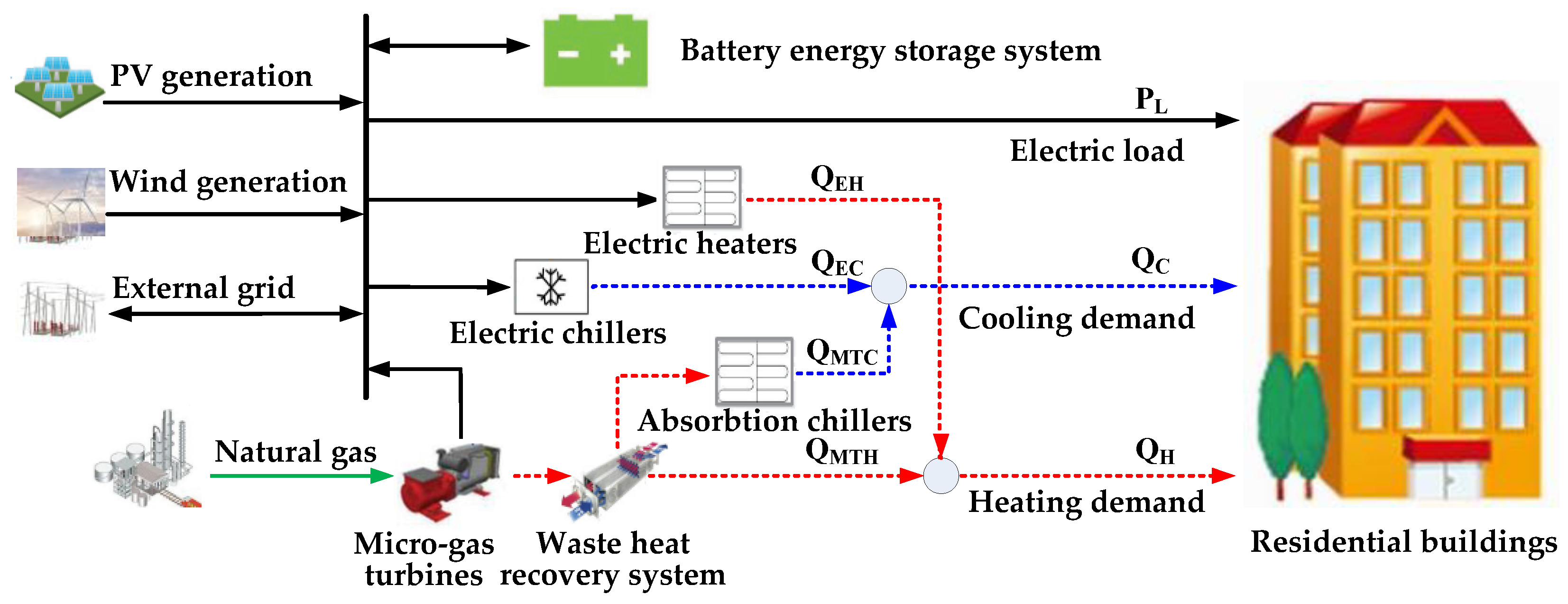
The structure of the RR-microgrid studied in this paper is shown in Figure 1, and it is known that the RR-microgrid consists of renewable DGs, such as photovoltaic generation (PV) and wind generation (WT), a battery energy storage system (BESS), a CCHP unit which is composed of micro-gas turbines (MTs), a waste heat recovery system (WHRS), absorption chillers (ACs), and other devices, like electric heaters (EHs) as well as electric chillers (ECs). In addition, the RR-microgrid is connected to an external grid so that the exchange of electric power is allowed. “Redundant” means that the heating/cooling demand of residential buildings could be satisfied by the CCHP unit as well as EHs/ECs, while the electric load of the residential buildings could be satisfied by clean energy generation, the external grid, and the CCHP unit.

2.2. Models of Energy Supplies

(1) CCHP Unit

MTs generate electricity through consuming natural gas, and the output electric power P_MT can be expressed as:

$$P_{\mathrm{MT}}^{}=F_{\mathrm{gas}}^{}\times L_{\mathrm{HVNG}}\times {\eta }_{\mathrm{MTE}}^{}$$

(1)

meanwhile, the output thermal power Q_MT is:

$$Q_{\mathrm{MT}}^{}=F_{\mathrm{gas}}^{}\times L_{\mathrm{HVNG}}\times {\eta }_{\mathrm{MTH}}^{}$$

(2)

where F_gas is natural gas MTs consumed per unit time, L_HVNG is the low calorific value for natural gas, and η_MTE and η_MTH are the electric power efficiency and thermal power efficiency for MTs, respectively.

Output thermal power Q_MT could be turned into the heating power Q_MTH by the WHRS:

$$Q_{\mathrm{MTH}}^{}=Q_{\mathrm{MT}}^{}\times {\eta }_{\mathrm{HE}}$$

(3)

where η_HE is the conversion efficiency of WHRS, and could be further turned into the cooling power Q_MTC by the ACs:

$$Q_{\mathrm{MTC}}^{}=Q_{\mathrm{MTH}}^{}\times \mathrm{C}\mathrm{O}{\mathrm{P}}_{\mathrm{AC}}$$

(4)

where COP_AC is coefficient of performance (COP) for ACs.

(2) Electric Heaters/Chillers

The EHs consume electric energy to generate the heating power Q_EH expressed as:

$$Q_{\mathrm{EH}}^{}=P_{\mathrm{EH}}^{}\times \mathrm{C}\mathrm{O}{\mathrm{P}}_{\mathrm{EH}}$$

(5)

where P_EH is the consumed electric power, COP_EH is the COP for EHs. The ECs consume electric energy to generate the cooling power Q_EC expressed as:

$$Q_{\mathrm{EC}}^{}=P_{\mathrm{EC}}^{}\times \mathrm{C}\mathrm{O}{\mathrm{P}}_{\mathrm{EC}}$$

(6)

where P_EC is the consumed electric power, COP_EC is the COP for ECs.

(3) Battery Energy Storage System

In practice, the charging and discharging processes of the BESS are usually not constant. However, for the sake of simplicity, the charging and discharging of the battery is regarded as a constant power load or supply during every scheduling period. The state of charge (SOC) for the BESS varies during charging/discharging process, which can be expressed as:

$$E_{}^t=E_{}^{t-1}+\Delta T\times {\mathrm{U}}_{\mathrm{Si}+}^t\times P_{\mathrm{Si}+}^t\times {\eta }_{\mathrm{c}}-\Delta T\times {\mathrm{U}}_{\mathrm{Si}-}^t\times \frac{P_{\mathrm{Si}-}^t}{{\eta }_{\mathrm{disc}}}$$

(7)

where $E_{}^t$ is the SOC at the end of scheduling period t, $E_{}^{t-1}$ is the SOC at the end of scheduling period t – 1, $P_{\mathrm{Si}+}^t/P_{\mathrm{Si}-}^t$ are the charging power and discharging power for scheduling period t, respectively, $U_{\mathrm{Si}+}^t/U_{\mathrm{Si}-}^t$ are the charging status and discharging status for scheduling period t, respectively, ${\eta }_{\mathrm{c}}/{\eta }_{\mathrm{disc}}$ are the charging efficiency and discharging efficiency, respectively, and $\Delta T$ is the time length of the scheduling period.

3. Equivalent Thermodynamic Parameters Model of the Heating/Cooling System in the RR-Microgrid

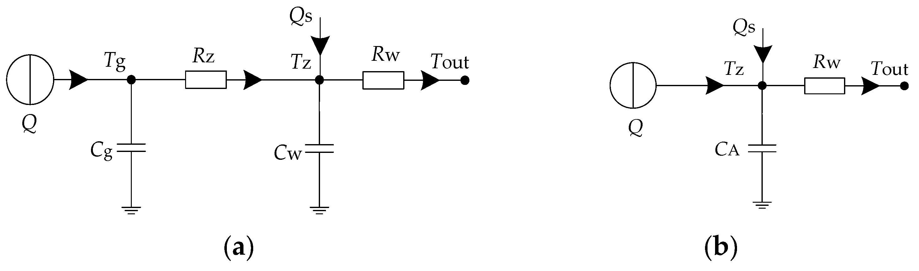
In this paper, two kinds of heating/cooling systems for residential buildings are investigated: the RFHCS as well as the CHCS. The RFHCS is different from CHCS in the way of transferring heat/cool to the human body, as the former does so mainly through thermal radiation of the floor and envelope structure, while the latter does so mainly through indoor air convection. Generally, the operative temperature is suitable to evaluate the TCL. Correspondingly, the mean value of the air temperature and indoor average radiation temperature could be regarded as the operative temperature for the RFHCS, while the indoor air temperature could be regarded as the operative temperature for the CHCS. The operative temperature is influenced mainly by the solar radiation load, heating/cooling demand, and the thermal runaway resulting from the difference between the indoor temperature and outdoor temperature. Accordingly, in this paper, equivalent thermodynamic parameter (ETP) models for the RFHCS and CHCS are established, respectively, to describe their mathematical relationships based on [16], as shown in Figure 2.

In Figure 2, Q and Q_s represent the heating/cooling demand (W) and solar radiation load (W), respectively; T_g, T_z, and T_out represent the radiant floor surface temperature (°C), the operative temperature (°C), and the outdoor temperature (°C), respectively, C_g, C_w, and C_A represent the equivalent heat capacities (J/°C) of the radiant floor, the envelope structure, and the indoor air, respectively; R_W represents the equivalent heat resistance (°C/W) for the envelope structure, while R_Z represents the equivalent heat resistance (°C/W) of convection and radiation from the radiant floor surface to the indoor air and envelope structure.

For RFHCS, the differential equations for corresponding ETP model are:

$$C_{\mathrm{g}}\frac{d{T}_{\mathrm{g}}}{dt}=Q-\frac{T_{\mathrm{g}}-T_{\mathrm{z}}}{R_{\mathrm{z}}}$$

(8)

$$C_{\mathrm{w}}\frac{d{T}_{\mathrm{z}}}{dt}=\frac{T_{\mathrm{g}}-T_{\mathrm{z}}}{R_{\mathrm{z}}}+Q_{\mathrm{s}}-\frac{T_{\mathrm{z}}-T_{\mathrm{out}}}{R_{\mathrm{w}}}$$

(9)

while for the CHCS, the differential equation for corresponding ETP model is:

$$C_{\mathrm{A}}\frac{d{T}_{\mathrm{z}}}{dt}=Q+Q_{\mathrm{s}}-\frac{T_{\mathrm{z}}-T_{\mathrm{out}}}{R_{\mathrm{w}}}$$

(10)

Taking into account the specific structure and material properties of residential buildings, Equations (8) and (9) can be converted to:

$$A_{\mathrm{g}}\times C_{\mathrm{g}1}^{}\times \frac{d{T}_{\mathrm{g}}}{dt}=Q-A_{\mathrm{g}}\times h_{\mathrm{z}}^{}(T_{\mathrm{g}}-T_{\mathrm{z}})$$

(11)

$$(A_{\mathrm{wi}}\times C_{\mathrm{wi}}+A_{\mathrm{wa}}\times C_{\mathrm{wa}})\frac{d{T}_{\mathrm{z}}}{dt}=A_{\mathrm{g}}{h}_{\mathrm{z}}^{}(T_{\mathrm{g}}-T_{\mathrm{z}})+A_{\mathrm{wi}}\times I\times \alpha -(A_{\mathrm{wi}}{k}_{\mathrm{wi}}+A_{\mathrm{wa}}{k}_{\mathrm{wa}})(T_{\mathrm{z}}-T_{\mathrm{out}})$$

(12)

while Equation (10) can be converted to:

$$\rho \times C\times V\times \frac{d{T}_{\mathrm{z}}}{dt}=Q+A_{\mathrm{wi}}\times I\times \alpha -(A_{\mathrm{wi}}{k}_{\mathrm{wi}}+A_{\mathrm{wa}}{k}_{\mathrm{wa}})(T_{\mathrm{z}}-T_{\mathrm{out}})$$

(13)

where A_g, A_wa, and A_wi represent the total area (m²) of the radiant floor, external walls, and external windows, respectively, in the residential building; C_g1, C_wa, and C_wi represent the equivalent heat capacity (kJ/(m²·°C)) of the radiant floor, external walls, and external windows, respectively; ρ, C, and V represent, respectively, the density (kg/m³), heat capacity (kJ/(kg·°C)), and volume (m³) of the indoor air; h_z represents the comprehensive heat transfer coefficient (W/m²·°C) from the radiant floor surface to the indoor air as well as the envelope structure; k_wi and k_wa represent the heat transfer coefficient (W/m²·°C) for the external walls and external windows of the envelope structure, respectively; I represents the total solar radiation intensity (W/m²); and α represents the shading coefficient of the residential building.

From Equations (11)–(13), it is known that owing to the heat capacity for the radiant floor, external windows, external walls, and indoor air, the heating/cooling demand could be adjusted to a certain extent while ensuring the operative temperature T_z changes within a reasonable range. Therefore, both the RFHCS and CHCS have charging/discharging characteristics, like the energy storage system, which could be considered as a virtual energy storage system (VESS).

4. Optimization Model for RR-Microgrid Scheduling

4.1. Optimized Variables

A day-ahead optimization model for scheduling of the RR-microgrid is presented based on MINLP, of which the time length of the scheduling period $\Delta T$ is 1 h and the number of the scheduling periods ${\theta }_T$ is 24. For the scheduling period $t\in {\theta }_T$, the variables that need to be optimized could be divided into control variables and state variables, as shown in

Table 1. Control variables.

Variables	Description
$P_{\mathrm{MT}}^t$	Output electric power of MTs
$P_{\mathrm{Si}+}^t$	Charging power for the BESS
$P_{\mathrm{Si}-}^t$	Discharging power for the BESS
$P_{\mathrm{grid}+}^t$	Electric power purchasing from the grid
$P_{\mathrm{grid}-}^t$	Electric power selling to the grid
$P_{\mathrm{EH}}^t$	Electric power consumed by the EHs
$P_{\mathrm{EC}}^t$	Electric power consumed by the ECs

and

Table 2. State variables.

Variables	Description
$Q_{\mathrm{MT}}^t$	Output thermal power for MTs
${\eta }_{\mathrm{MTE}}^t$	Electric power efficiency for MTs
$E_{}^t$	SOC for the BESS
$T_{\mathrm{g}}^t$	Surface temperature of the radiant floor
$T_{\mathrm{z}}^t$	Operative temperature of the residential building

, respectively.

4.2. Objective Function

In this paper, there are three optimization objectives considered for RR-microgrid scheduling: operating cost (OC), thermal comfort level (TCL), and pollution emission (PE).

4.2.1. Objective Function for Operating Cost

The OC of the RR-microgrid consists of four parts: the consuming cost of natural gas, the charging/discharging cost of the BESS, the cost of exchanging electric power with the external grid, and the maintenance cost of clean energy generation and devices, of which the objective function is expressed as:

$$\min f_2(x_{\mathrm{s}})=f_{\mathrm{G}}(x_{\mathrm{s}})+f_{\mathrm{S}}(x_{\mathrm{s}})+f_{\mathrm{Grid}}(x_{\mathrm{s}})+f_{\mathrm{RMC}}(x_{\mathrm{s}})$$

(14)

In Equation (15), f_G is consuming cost of natural gas:

$$f_{\mathrm{G}}(x_{\mathrm{s}})={\displaystyle \sum _{t\in {\theta }_{\mathrm{T}}}{c}_{\mathrm{gas}}^{}{F}_{\mathrm{gas}}^t}$$

(15)

where $c_{\mathrm{gas}}^{}$ is the price for natural gas, $F_{\mathrm{gas}}^t$ is the natural gas MTs consumed at scheduling period t.

f_S is charging/discharging cost of the BESS:

$$f_{\mathrm{S}}(x_{\mathrm{s}})={\displaystyle \sum _{t\in {\theta }_{\mathrm{T}}}(c_{\mathrm{Si}+}^{}{P}_{\mathrm{Si}+}^t+c_{\mathrm{Si}-}^{}{P}_{\mathrm{Si}-}^t)\Delta T}$$

(16)

where $c_{\mathrm{Si}+}^{}$ and $c_{\mathrm{Si}-}^{}$ are the unit costs for charging/discharging.

f_Grid is cost of exchanging electric power with external grid:

$$f_{\mathrm{Grid}}(x_s)={\displaystyle \sum _{t\in {\theta }_{\mathrm{T}}}(c_{\mathrm{grid}+}^t{P}_{\mathrm{grid}+}^t-c_{\mathrm{grid}-}^t{P}_{\mathrm{grid}-}^t)}\Delta T$$

(17)

where $c_{\mathrm{grid}+}^t$ and $c_{\mathrm{grid}-}^t$ are the prices for purchasing/selling electricity from the external grid at scheduling period t.

f_RMC is maintenance cost of clean energy generation and devices:

$$f_{\mathrm{RMC}}(x_{\mathrm{s}})={\displaystyle \sum _{t\in {\theta }_{\mathrm{T}}}(c_{\mathrm{WT}}^{}{P}_{\mathrm{WT}}^t+c_{\mathrm{PV}}^{}{P}_{\mathrm{PV}}^t+c_{\mathrm{MT}}^{}{P}_{\mathrm{MT}}^t+c_{\mathrm{EH}}^{}{P}_{\mathrm{EH}}^t+}{c}_{\mathrm{EC}}^{}{P}_{\mathrm{EC}}^t+c_{\mathrm{AC}}^{}{Q}_{\mathrm{MTC}}^t)\Delta T$$

(18)

where $P_{\mathrm{WT}}^t$ and $P_{\mathrm{PV}}^t$ are, respectively, the output power of WT and PV at scheduling period t, $c_{\mathrm{WT}}^{}$, $c_{\mathrm{PV}}^{}$, $c_{\mathrm{MT}}^{}$, $c_{\mathrm{EH}}^{}$, $c_{\mathrm{EC}}^{}$ and $c_{\mathrm{AC}}^{}$ are, respectively, the unit maintenance cost for WT, PV, MTs, EHs, ECs, and ACs.

4.2.2. Objective Function for the Thermal Comfort Level

Ref. [28] presented the predicted mean vote (PMV) as well as the predicted percentage of dissatisfied (PPD) to describe peoples’ subjective perception to the thermal environment. According to the national standards of the PRC (GB/T 18049-2000), the reasonable scopes of PMV and PPD are: PPD ≤ 27%, −1 ≤ PMV ≤ +1. It is calculated in [27] that, in winter, the optimum operative temperature T_zopt is about 22 °C, while in summer it is about 25 °C, corresponding to PMV = 0. In winter the variation range of T_z is 17~27 °C, while in summer is 21.5~29 °C, corresponding to PPD ≤ 27%, −1 ≤ PMV ≤ +1, which proves it is feasible to adjust the heating/cooling demand for economic benefits.

In the presented optimization model, the permitted adjustable scope of T_z during the scheduling is ±2.5 °C to guarantee the TCL, and the objective function for the TCL is expressed as quadratic sum of deviations between the optimum value and the actual value of the operative temperature during all scheduling periods:

$$\min f_1(x_{\mathrm{s}})={\displaystyle \sum _{t\in {\theta }_{\mathrm{T}}}{\left|T_{\mathrm{z}}^t-T_{\mathrm{zopt}}^{}\right|}^2}$$

(19)

4.2.3. Objective Function for Pollution Emission

The PE mainly includes the emission from the consumption of electricity purchased from the external grid and the emission from consumption of natural gas. In this paper, the electricity purchasing from the external grid is assumed generated by coal-fired power stations. Three types of polluting gas are taken into account for consumption of coal and natural gas, i.e., CO₂, SO₂, and NO_x, as shown in

Table 3. Emission coefficients of natural gas and coal [29].

Pollution Gas	CO2	SO2	NOx	Total
Coal (kg/(MWh))	326.37	3.14	1.134	330.644
Natural Gas (kg/(MWh))	203.74	0.011	0.202	203.953

. Consequently, the objective function for PE is depicted in Equation (20):

$$\min f_3(x_s)={\displaystyle \sum _{t\in {\theta }_{\mathrm{T}}}(P_{\mathrm{grid}+}^t{\lambda }_e+F_{\mathrm{gas}}^t{\lambda }_g)}\Delta T$$

(20)

where ${\lambda }_e$ and ${\lambda }_g$ are the total emission coefficients for coal consumption and natural gas consumption, respectively.

4.3. Constraints

(1) Balance of electric power:

$$P_{\mathrm{load}}^t+P_{\mathrm{EH}}^t+P_{\mathrm{EC}}^t+P_{\mathrm{Si}+}^t-P_{\mathrm{Si}-}^t=P_{\mathrm{PV}}^t+P_{\mathrm{WT}}^t+P_{\mathrm{MT}}^t+P_{\mathrm{grid}+}^t-P_{\mathrm{grid}-}^t,\forall t\in {\theta }_{\mathrm{T}}$$

(21)

where $P_{\mathrm{load}}^t$ is the forecast value of electric load at scheduling period t (electric power consumed by EHs/ECs is not taken into account).

(2) Balance of thermal power

Considering the process of thermal runaway and operative temperature fluctuation in residential building are quite slow, for the convenience of solving the presented optimization model, Equations (11)–(13) are transformed to be difference equations expressing the constraint of the thermal power balance for the RR-microgrid:

$$T_{\mathrm{g}}^{t+1}=T_{\mathrm{g}}^t+\frac{\Delta T}{A_{\mathrm{g}}{C}_{\mathrm{g}1}^{}}\times [Q_{}^t-A_{\mathrm{g}}{h}_{\mathrm{z}}^{}(T_{\mathrm{g}}^t-T_{\mathrm{z}}^t)],\forall t\in {\theta }_{\mathrm{T}}$$

(22)

$$T_{\mathrm{z}}^{t+1}=T_{\mathrm{z}}^t+\frac{\Delta T}{(A_{\mathrm{wi}}{C}_{\mathrm{wi}}+A_{\mathrm{wa}}{C}_{\mathrm{wa}})}\times [A_{\mathrm{g}}{h}_{\mathrm{z}}^{}(T_{\mathrm{g}}^t-T_{\mathrm{z}}^t)+A_{\mathrm{wi}}\times I_{}^t\times \alpha -(A_{\mathrm{wi}}{k}_{\mathrm{wi}}+A_{\mathrm{wa}}{k}_{\mathrm{wa}})(T_{\mathrm{z}}^t-T_{\mathrm{out}}^t)],\forall t\in {\theta }_{\mathrm{T}}$$

(23)

$$T_{\mathrm{z}}^{t+1}=T_{\mathrm{z}}^t+\frac{\Delta T}{\rho \times C\times V}\times [Q^t+A_{\mathrm{wi}}\times I_{}^t\times \alpha -(A_{\mathrm{wi}}{k}_{\mathrm{wi}}+A_{\mathrm{wa}}{k}_{\mathrm{wa}})(T_{\mathrm{z}}^t-T_{\mathrm{out}}^t)],\forall t\in {\theta }_{\mathrm{T}}$$

(24)

where for heating in winter, there is:

$$Q_{}^t=Q_{\mathrm{MT}}^t{\eta }_{\mathrm{HE}}+P_{\mathrm{EH}}^t\mathrm{C}\mathrm{O}{\mathrm{P}}_{\mathrm{EH}},\forall t\in {\theta }_{\mathrm{T}}$$

(25)

while for cooling in summer, there is:

$$Q_{}^t=-Q_{\mathrm{MT}}^t{\eta }_{\mathrm{HE}}\mathrm{C}\mathrm{O}{\mathrm{P}}_{\mathrm{AC}}-P_{\mathrm{EC}}^t\mathrm{C}\mathrm{O}{\mathrm{P}}_{\mathrm{EC}},\forall t\in {\theta }_{\mathrm{T}}$$

(26)

(3) Battery energy storage system

Uniqueness constraints for charging/discharging states of the BESS are expressed as:

$$P_{\mathrm{Si}+}^t{P}_{\mathrm{Si}-}^t=0,P_{\mathrm{Si}+}^t\ge 0,P_{\mathrm{Si}-}^t\ge 0,\forall t\in {\theta }_{\mathrm{T}}$$

(27)

Meanwhile, the charging/discharging power should satisfy the upper limits as:

$$P_{\mathrm{Si}+}^t\le \overline{P_{\mathrm{Si}+}},\forall t\in {\theta }_{\mathrm{T}}$$

(28)

$$P_{\mathrm{Si}-}^t\le \overline{P_{\mathrm{Si}-}},\forall t\in {\theta }_{\mathrm{T}}$$

(29)

and the SOC should satisfy upper/lower limits as:

$$\underset{\_}{E}\le E_{}^t\le \overline{E},\forall t\in {\theta }_{\mathrm{T}}$$

(30)

where $\overline{P_{\mathrm{Si}+}^{}}$ and $\overline{P_{\mathrm{Si}-}^{}}$ are, respectively, the upper limit for charging power and discharging power, while $\overline{E}$ and $\underset{\_}{E}$ are, respectively, the upper limit and lower limit for the SOC.

At the end of the last scheduling period, the SOC of the BESS should be equal with the initial value to ensure the balance of energy:

$$E_{}^0=E_{}^N$$

(31)

(4) Power exchanged with the external grid

The uniqueness constraints for power exchanged with external grid are expressed as:

$$P_{\mathrm{grid}+}^t{P}_{\mathrm{grid}-}^t=0,P_{\mathrm{grid}+}^t\ge 0,P_{\mathrm{grid}-}^t\ge 0,\forall t\in {\theta }_{\mathrm{T}}$$

(32)

Meanwhile, the power exchanged should satisfy the upper limits:

$$P_{\mathrm{grid}+}^t\le \overline{P_{\mathrm{grid}+}},\forall t\in {\theta }_{\mathrm{T}}$$

(33)

$$P_{\mathrm{grid}-}^t\le \overline{P_{\mathrm{grid}-}^{}},\forall t\in {\theta }_{\mathrm{T}}$$

(34)

where $\overline{P_{\mathrm{grid}+}^{}}$ and $\overline{P_{\mathrm{grid}-}^{}}$ are the upper limit, respectively, for power purchasing from, and selling to, the external grid.

(5) Micro-gas turbines

Output electric power for MTs should satisfy the upper limits:

$$P_{\mathrm{MT}}^t\le \overline{P_{\mathrm{MT}}^{}},\forall t\in {\theta }_{\mathrm{T}}$$

(35)

where $\overline{P_{\mathrm{MT}}^{}}$ is the upper limit for the output electric power for MTs.

In practice, the relationship between η_MT and P_MT is nonlinear. In the presented optimization model, the fourth-order polynomial is chosen to fit the relationship in order to facilitate subsequent calculation. Thus, the obtained polynomial equation could be expressed as:

$${\eta }_{\mathrm{MT}}^t={\alpha }_1{(\frac{P_{\mathrm{MT}}^t}{P_{\mathrm{MT}}^{\max }})}^4+{\alpha }_2{(\frac{P_{\mathrm{MT}}^t}{P_{\mathrm{MT}}^{\max }})}^3+{\alpha }_3{(\frac{P_{\mathrm{MT}}^t}{P_{\mathrm{MT}}^{\max }})}^2+{\alpha }_4(\frac{P_{\mathrm{MT}}^t}{P_{\mathrm{MT}}^{\max }})+{\alpha }_5,\forall t\in {\theta }_{\mathrm{T}}$$

(36)

where α₁, α₂, α₃, α₄, and α₅ are the fitting coefficients and $P_{\mathrm{MT}}^{\max }$ is the rated power.

(6) Electric heaters and electric chillers

Electric power EHs/ECs consumed should satisfy the upper limits:

$$P_{\mathrm{EH}}^t\le \overline{P_{\mathrm{EH}}^{}},\forall t\in {\theta }_{\mathrm{T}}$$

(37)

$$P_{\mathrm{EC}}^t\le \overline{P_{\mathrm{EC}}^{}},\forall t\in {\theta }_{\mathrm{T}}$$

(38)

where $\overline{P_{\mathrm{EH}}^{}}$ and $\overline{P_{\mathrm{EC}}^{}}$ are the upper limits for electric power consumed by EHs/ECs, respectively.

(7) Operative temperature

$$\underset{\_}{T_{\mathrm{z}}^{}}\le T_{\mathrm{z}}^t\le \overline{T_{\mathrm{z}}^{}},\forall t\in {\theta }_{\mathrm{T}}$$

(39)

where $\overline{T_{\mathrm{z}}^{}}$ and $\underset{\_}{T_{\mathrm{z}}^{}}$ are, respectively, the upper and lower limits of the operative temperature.

At the end of the last scheduling period, the operative temperature must be equal with the initial value for balance of thermal energy stored in residential building:

$$T_z^0=T_z^N$$

(40)

In addition, in order to prevent the appearance of condensation for cooling in summer, the surface temperature of the radiant floor is required to be higher than the dewpoint temperature:

$$T_{\mathrm{g}}^t>\underset{\_}{T_{\mathrm{g}}^{}},\forall t\in {\theta }_{\mathrm{T}}$$

(41)

where $\underset{\_}{T_{\mathrm{g}}^{}}$ is the dewpoint temperature.

5. Solve the Optimization Model Using NSGA-II and AHP

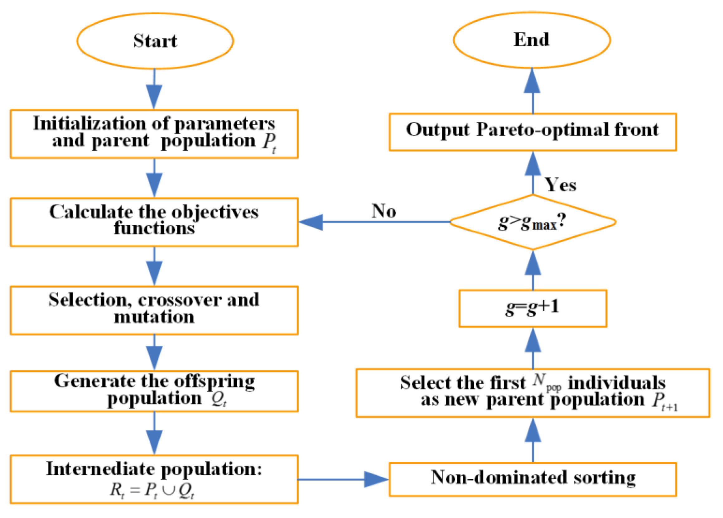
A genetic algorithm (GA) is a kind of population-based search algorithm which is quite suitable for solving multi-objective optimization problems. The NSGA-II algorithm is one of the most effective and efficient multi-objective optimization algorithms [30]. Compared with the NSGA algorithm, the NSGA-II algorithm has a better sorting method and incorporates elitism, while no sharing parameters need to be chosen. According to the non-domination concept, the populations are combined and sorted at each generation. The N least crowded solutions are chosen based on the crowding distance and abandons the rest of the non-dominated solutions. Owing to the above improvements, both spreading and convergence are ensured for the solution front without requiring any external population [31]. The flowchart of the NSGA-II algorithm is shown in Figure 3.

The steps of the NSGA-II algorithm are as follows:

(1)

Start, input basic system data.

(2)

Initialize parameters of the NSGA-II algorithm which consist of the number of individuals in the population, N_p, the maximum number of generations, g_max, the crossover probability, p_c, the mutation probability p_m, and generate N_p individuals randomly as the parent population, P_t.

(3)

Calculate the objective functions, and generate the offspring population Q_t from P_t using selection, crossover, and mutation operators.

(4)

Create the intermediate population $R_t=P_t\cup Q_t$.

(5)

Perform a non-dominated sorting to R_t based on the calculation of the crowding distance and check constraints.

(6)

Select the first N_p individuals as new parent population P_t+1.

(7)

Check whether the result is equal with the maximum number of generations. If not, return to Step (3), otherwise continue to Step (8).

(8)

Output the Pareto-optimal front.

The final output of above NSGA-II algorithm is the Pareto front which represents a set of non-dominated solutions, and the last step is to determine a solution representing the best scheduling, which is called multi-objective decision making (MODM). There are different methods that can be adopted for MODM, and the AHP method is utilized in this paper. The main steps of the AHP method are as follows: Above all, the relative importance of each objective is judged in accordance with the fundamental scale defined in [32], a pairwise comparison matrix B is constructed, like in Equation (42), and the largest eigenvalue λ_max and corresponding normalized eigenvectors set ω are calculated. Then, the consistency check of B is performed to ensure the process of the AHP method is effective. Finally, ω is taken as the set of weight of each objective, as shown in Equation (43):

$$B=\left[\begin{array}{ccc}1& 3& 5\\ 1/3& 1& 3\\ 1/5& 1/3& 1\end{array}\right]$$

(42)

$${\mathsf{\lambda }}_{\max }=3.0385,\omega =\{0.6090,0.2793,0.1116\}$$

(43)

6. Case Study

In order to validate the feasibility and validity of the proposed scheduling method for the RR-microgrid, a case study is performed respectively considering scenes of heating in winter as well as cooling in summer.

6.1. Case Introduction

Take a residential building (30 m long, 20 m wide, and 70 m high) consisting of 100 households as an example, like in [27], the total areas of the envelope structure and radiant floor are 7100 m² and 10,600 m², respectively, while the shading coefficient α is 0.2 and the window-to-wall ratio is 0.3. Material properties of the RFHCS and the envelope structure of the residential building are shown in

Table 4. Structure and material properties of RFHCS [33].

Type	Structure and Materials	Comprehensive Heat Transfer Coefficient (W/(m2·°C))	Equivalent Heat Capacity (kJ/(m2·°C))
Heavy floor	25 mm cement mortar +25 mm marble + 70 mm concrete (embedded diameter 20 mm pipe, spacing 150 mm)	11	148.1

and

Table 5. Structure and material properties of the envelope structure [25].

Type	Structure and Materials	Heat Transfer Coefficient (W/(m2·°C))	Equivalent Heat Capacity (kJ/(m2·°C))
External window	ordinary hollow glass + PV plastic window	2.80	6.0
External wall	25 mm cement mortar + 190 mm single row hole block + 25 mm adiabatic mortar	1.50	62

, respectively.

The specifications of the MTs, BESS, EHs, ECs, WT, and PV in the RR-microgrid are shown in

Table 6. Specification of MTs.

Type	Number of Units	$\overline{{\mathit{P}}_{\mathbf{MT}}^{}}\left(\mathbf{kW}\right)$	${\mathit{c}}_{\mathbf{MT}}(\mathbf{CNY}/\mathbf{MWh})$	${\mathit{\eta }}_{\mathbf{MTH}}$	${\mathit{\eta }}_{\mathbf{HE}}$
C200	3	600	30	0.53	0.95

,

Table 7. Specification of the BESS.

${\mathit{\eta }}_{\mathbf{c}}/{\mathit{\eta }}_{\mathbf{disc}}$	$\overline{{\mathit{P}}_{\mathbf{Si}+}^{}}\left(\mathbf{kW}\right)$	$\overline{\mathit{E}}\left(\mathbf{kWh}\right)$	$\underset{\_}{\mathit{E}}\left(\mathbf{kWh}\right)$	${\mathit{E}}^0\left(\mathbf{kWh}\right)$	${\mathit{c}}_{\mathbf{Si}+}/{\mathit{c}}_{\mathbf{Si}-}$
0.9	80	550	50	150	0.01

,

Table 8. Specification of EHs.

Type	$\overline{{\mathit{P}}_{\mathbf{EH}}^{}}\left(\mathbf{kW}\right)$	${\mathbf{COP}}_{\mathbf{EH}}$	${\mathit{c}}_{\mathbf{EH}}(\mathbf{CNY}/\mathbf{MWh})$
CWDZ1080-85/70	1080	0.99	10

,

Table 9. Specification of ECs.

$\overline{{\mathit{P}}_{\mathbf{EC}}^{}}\left(\mathbf{kW}\right)$	${\mathbf{COP}}_{\mathbf{EC}}$	${\mathit{c}}_{\mathbf{EC}}(\mathbf{CNY}/\mathbf{MWh})$
1000	4	10

and

Table 10. Specification of WT and PV.

Type	Rated Power (kW)	Maintenance Cost (CNY/MWh)
WT	400	110
PV	300	80

. The price of natural gas c_gs is 2.4 CNY/m³, and the calorific value L_HVNG is 34.92 MJ/m³. The upper limits of power purchasing from and selling to the external grid are $\overline{P_{\mathrm{grid}+}^{}}=\overline{P_{\mathrm{grid}-}^{}}=1000\mathrm{kW}$.

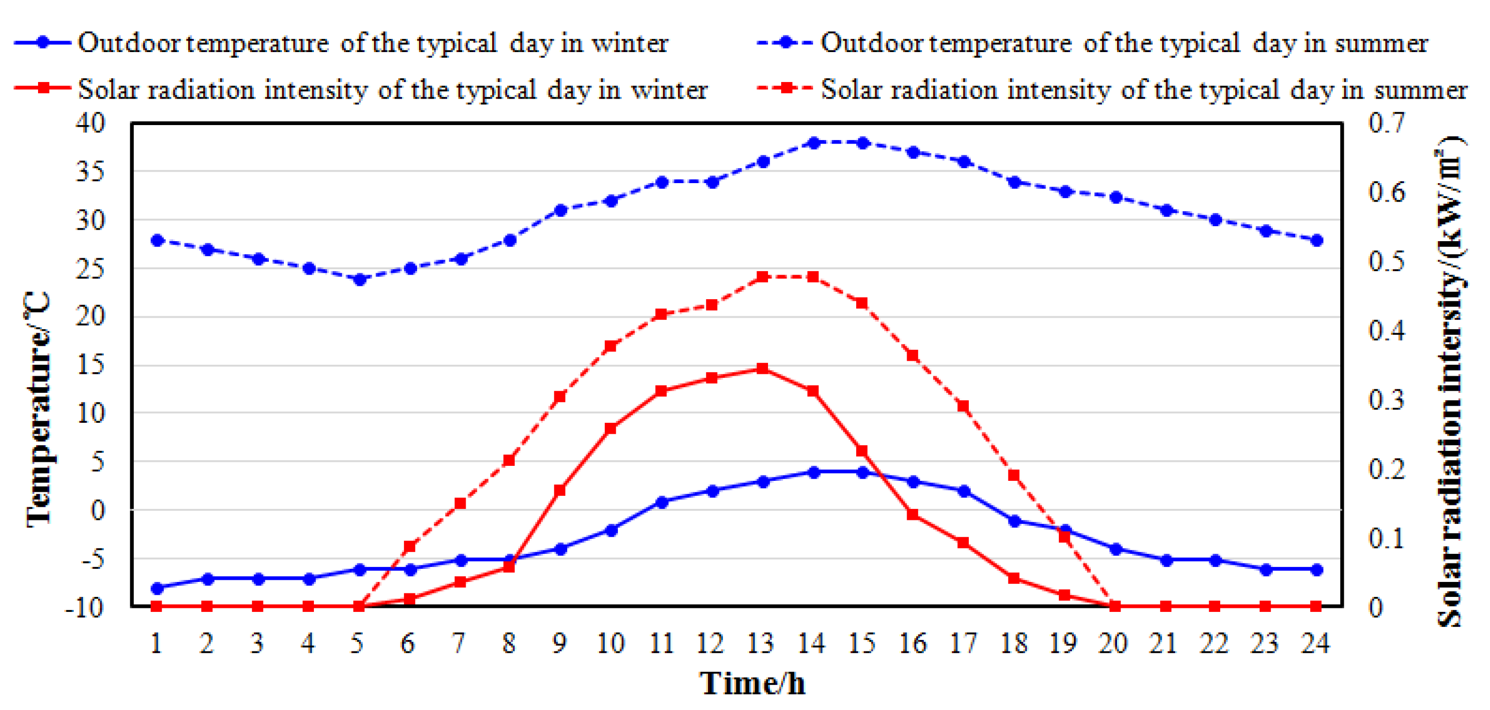
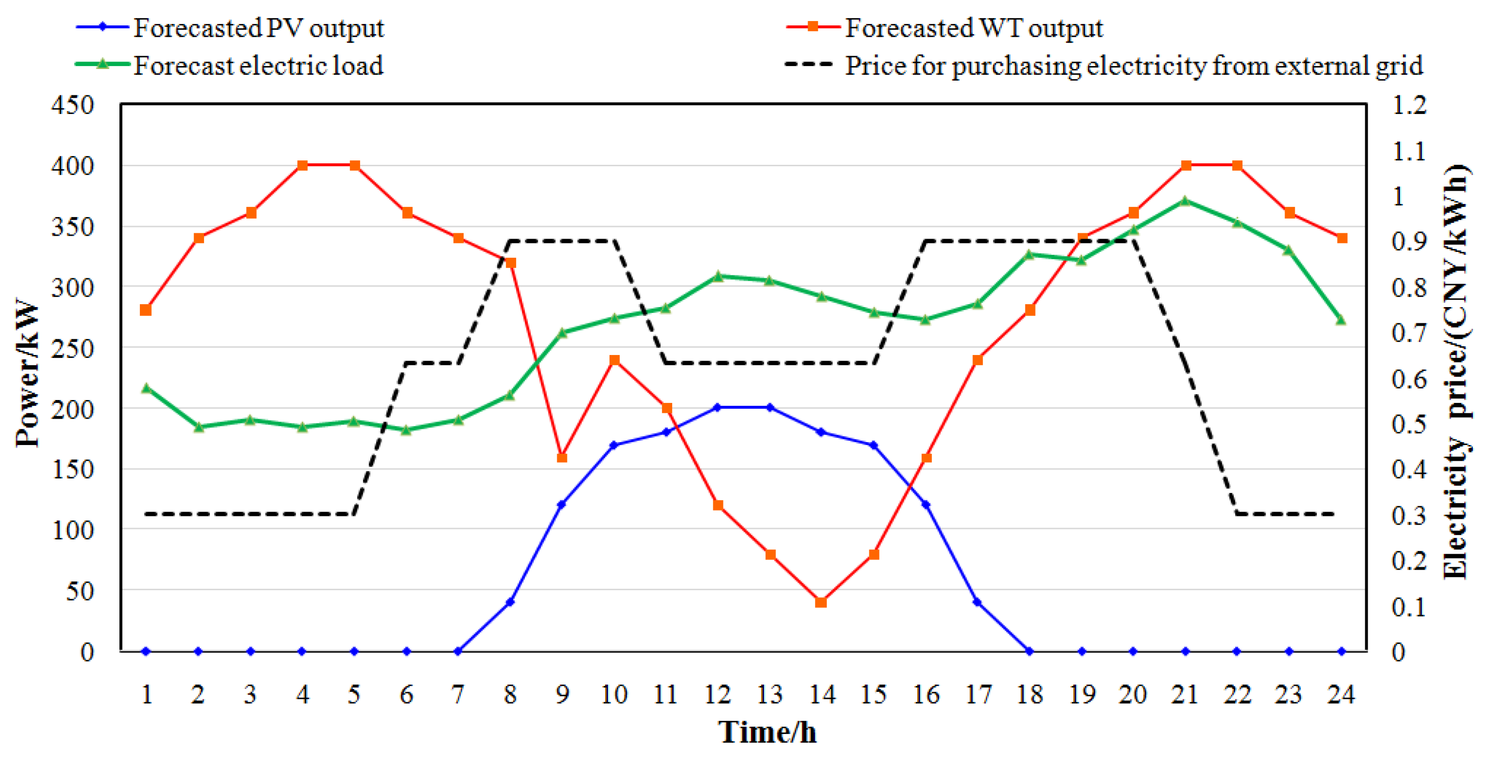
Typical days in summer and in winter are chosen to carry out the scheduling experiment in Hebei Province of China, while the corresponding forecasted curves of solar radiation intensity and outdoor temperature are shown in Figure 4, forecasted curves of WT output, PV output, electric load, and price curves of purchasing electricity from the external grid are shown in Figure 5. The peak-valley purchasing electricity price curves released by Hebei Southern Grid is utilized for the scheduling experiment, while the selling electricity price is set to be 80% of the purchasing electricity price.

The solving process of the presented optimization model for the RR-microgrid is implemented using MATLAB software from MathWorks Company of America. Set the parameters of the NSGA-II algorithm as: individual number in the population N_p = 200, maximum number of generation g_max = 60,000, crossover probability p_c = 0.9, and mutation probability p_m = 0.5.

6.2. Analysis of Scheduling Results

Optimal scheduling results are analyzed, respectively, for the RR-microgrid with RFHCS and the RR-microgrid with CHCS in this paper.

6.2.1. Scheduling Results of RR-Microgrid with RFHCS

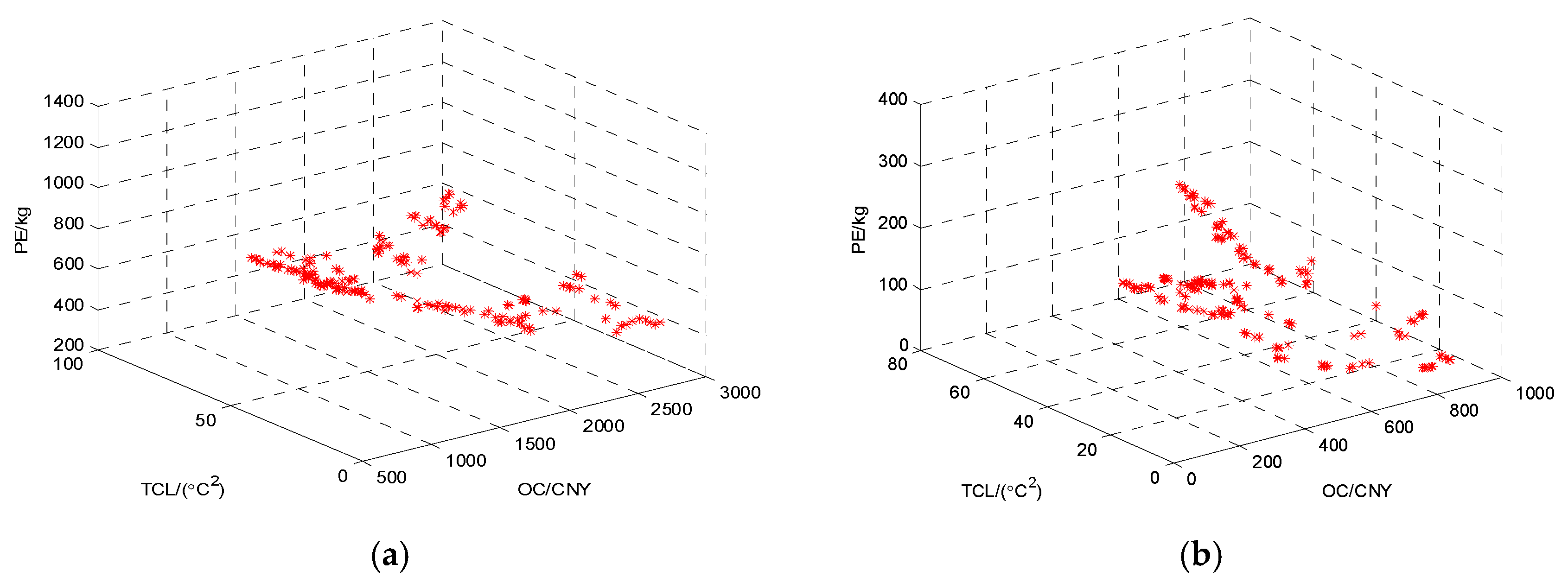
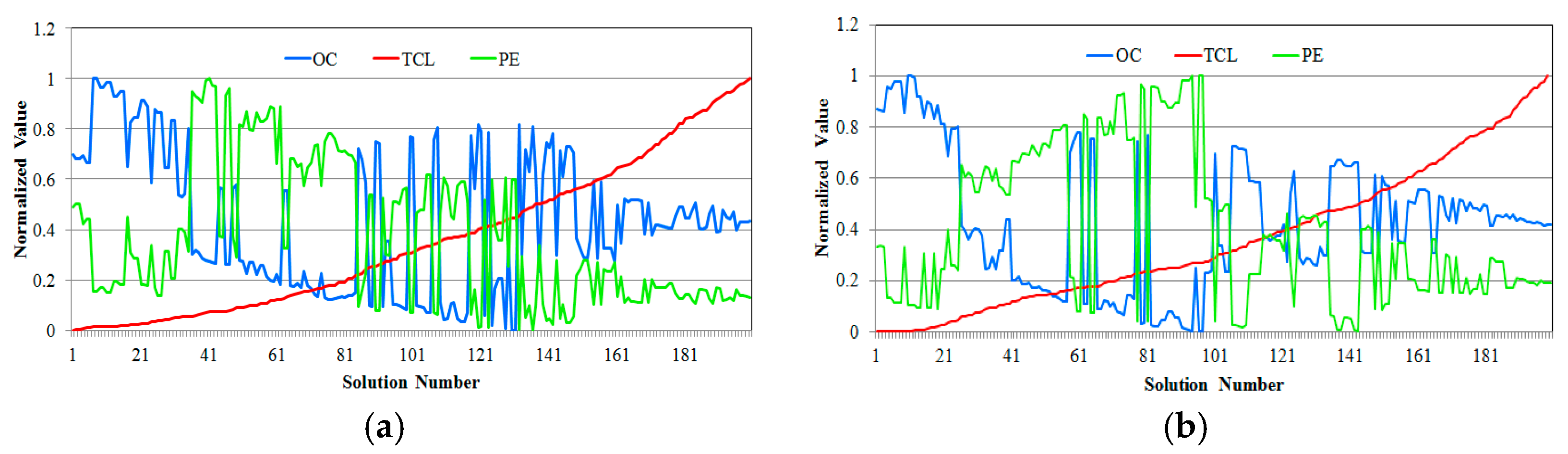
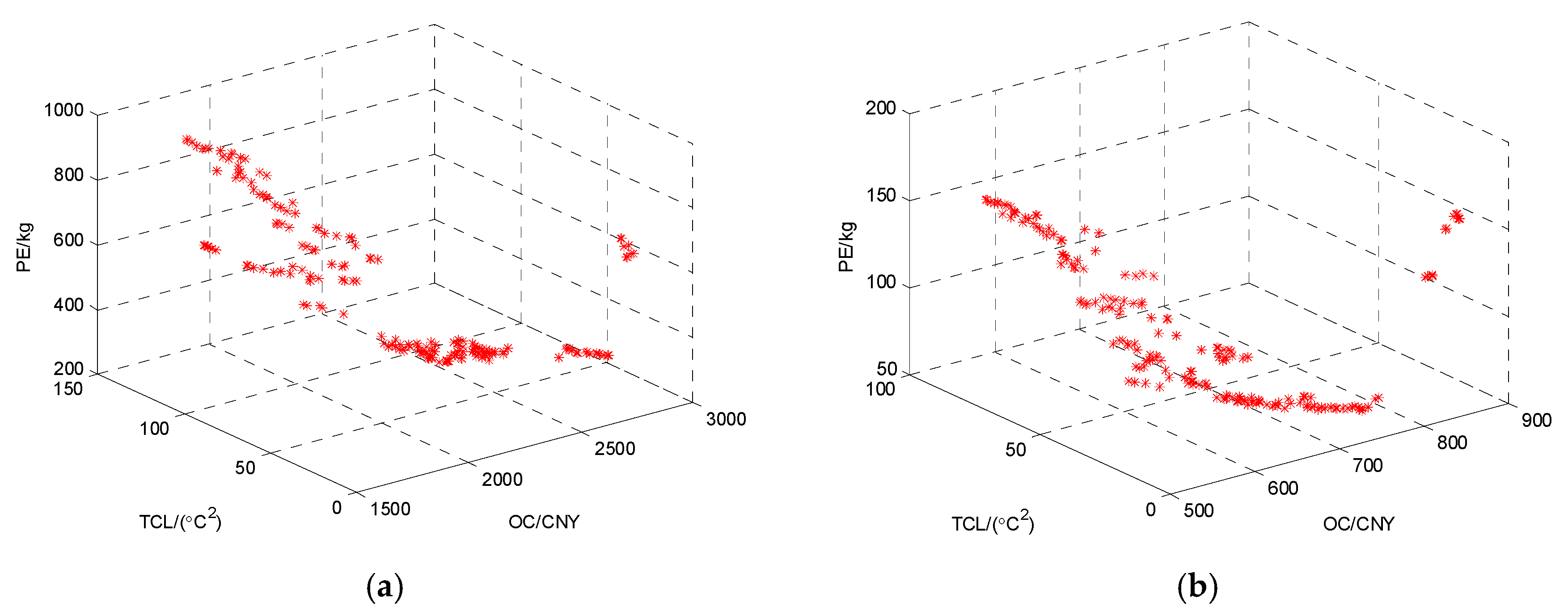
The Pareto-optimal front of the presented multi-objective optimization model obtained by NSGA-II algorithm is shown in Figure 6. It is known that the Nhe edges SGA-II algorithm could gain enough optimal scheduling solutions, and the solution, which is at t of the Pareto-optimal front represent optimal scheduling schemes for minimized OC, TCL, and PE, respectively. The normalized objectives of the Pareto-optimal front sorted by TCL are shown in Figure 7 and, obviously, the OC and PE are two opposite objectives where increasing one of them decreases the other one when TCL is invariable.

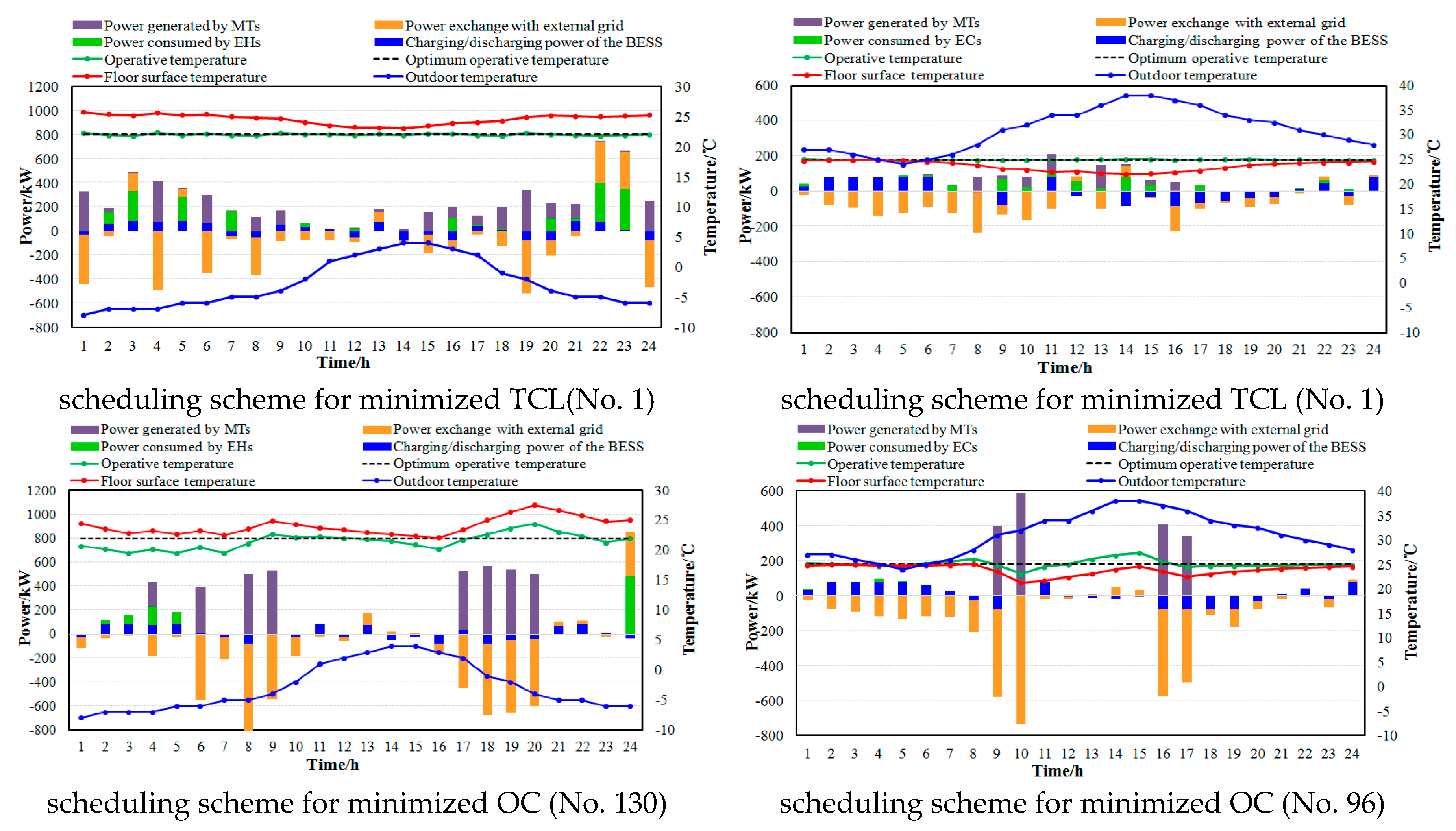
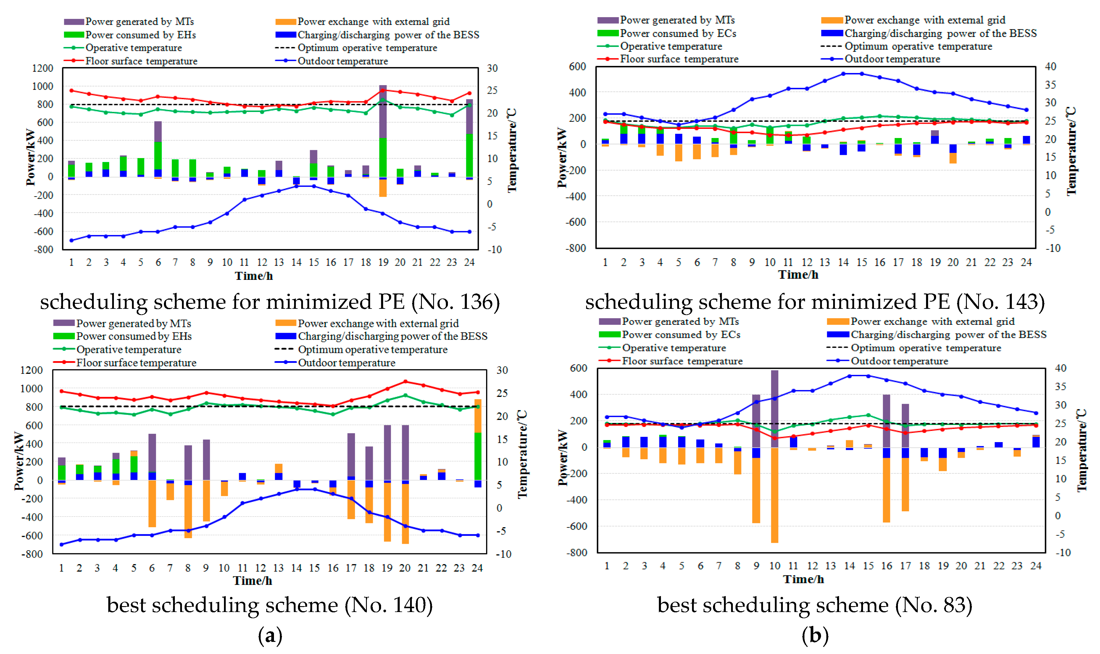
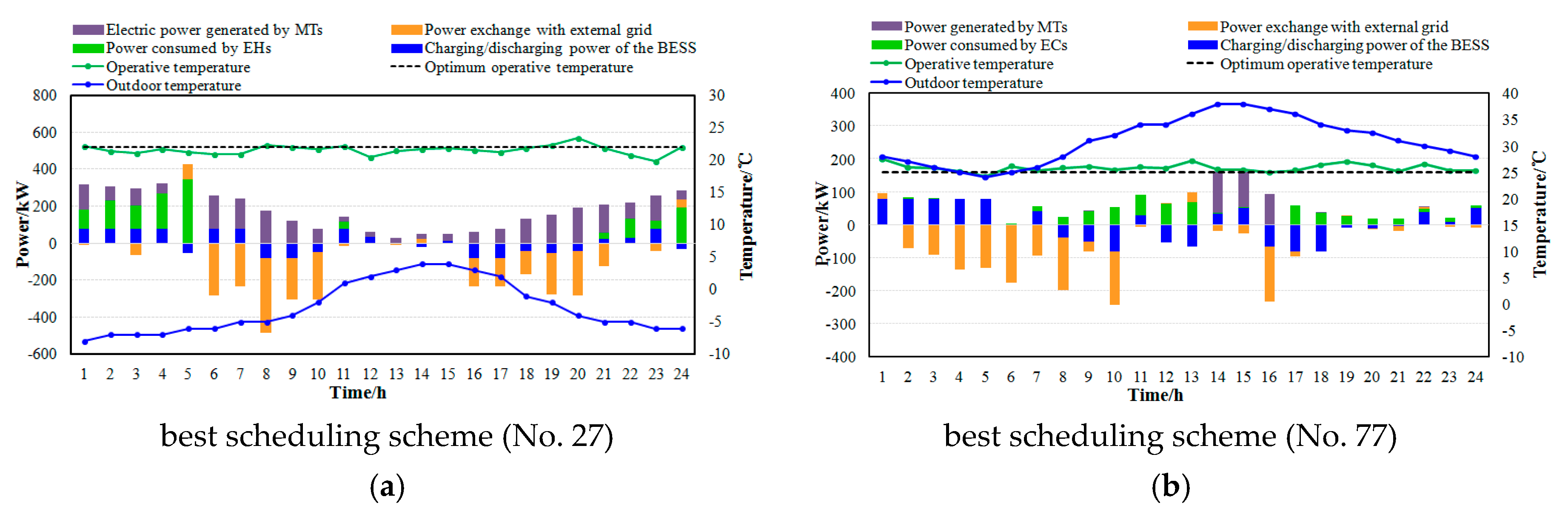
The optimal scheduling schemes for minimized TCL, OC, PE, as well as the best scheduling scheme determined by AHP method are shown in Figure 8, in which the discharging power of the BESS as well as the electric power selling to the external grid are taken as negative for the convenience of representation, and the corresponding value of the objectives are shown in

Table 11. Value of objective functions of different scheduling schemes for the typical day in winter.

Objective Functions	OC (CNY)	TCL (°C2)	PE (kg)
No. 1	2103.56	0.69	840.71
No. 130	736.49	44.65	949.51
No. 136	2326.27	48.89	348.62
No. 140	927.67	25.26	888.73

and

Table 12. Value of objective functions of different scheduling schemes for the typical day in summer.

Objective Functions	OC (CNY)	TCL (°C2)	PE (kg)
No. 1	759.75	0.09	135.97
No. 96	184.77	17.38	387.96
No. 143	623.80	31.87	9.46
No. 83	197.6	15.62	372.19

.

For all above scheduling schemes, the charging/discharging behaviors of the BESS are mainly effected by electricity price, that is, the charging behavior prefers to happen during lower price periods (0:00–5:00, 21:00–24:00), while the discharging behavior prefers to happen during higher price periods (7:00–10:00, 15:00–20:00), which is a benefit to the economy of the RR-microgrid, obviously.

As for the scheduling scheme for minimized TCL, it is observed that the operative temperature is quite close to the optimum operative temperature for all scheduling periods, which indicates that the thermal power generated by MTs and EHs/ECs could satisfy the heating/cooling demand quite well. According to the time-varying characteristic of the outdoor temperature, as well as solar radiation intensity, it is easily deduced theoretically that the cooling demand in summer concentrates on the daytime while the heating demand in winter concentrates on the nighttime. In addition, the heating demand in winter is obviously greater than the cooling demand in summer mainly because the difference between indoor temperature and outdoor temperature in winter is greater than in summer. The distribution characteristic of electric power generated by MTs and power consumed by EHs/ECs on typical days in winter/summer agree quite well with the above-mentioned conclusion.

As for the scheduling scheme for minimized OC, on the typical day in winter, the EHs only consume power during lower price periods, while the MTs mainly work during higher price periods for at these time they could achieve better economy, respectively; on the typical day in summer, since to the cooling demand of the nighttime is quite small, the ECs almost stop work for all periods, while the MTs only work during higher price periods in daytime. On the whole, during lower price periods, less thermal energy are generated by MTs and EHs/ECs, therefore operative temperature falls slowly or maintains at a low level on the typical day in winter while it rises slowly or maintains at a high level on the typical day in summer; on the contrary, during higher price periods, more thermal power is generated by MTs and EHs/ECs, therefore, the operative temperature rises slowly on the typical day in winter while it falls slowly on the typical day in summer. Obviously, to achieve the minimized OC, there is little electric power purchasing from the external grid on the whole, but quite a lot of electric power selling to the external grid during higher price periods. It should be realized that both the MTs and EHs/ECs nearly stop working during the middle price periods (10:00–15:00) for typical days in winter/summer, which indicates that the RFHCS is able to pre-store considerable heat/cool energy enough to maintain the operating temperature within a reasonable scope for the next several scheduling periods.

As for the scheduling scheme for minimized PE, for both typical days, no electric power is purchased from the grid due to the coal consumption having greater a total emission coefficient than natural gas. Meanwhile, the electric power selling to the grid is obviously less than that of the scheduling schemes for minimized OC and TCL.

As for the best scheduling scheme determined by the AHP method, the variation trend of the operative temperature is quite similar with that of the scheduling scheme for minimized OC, while smaller TCL and PE are achieved through the power redistribution between EHs/ECs and MTs. Obviously, it is essentially a compromise scheduling scheme with overall consideration of multi-objectives according to the set of weight of each objective in AHP method.

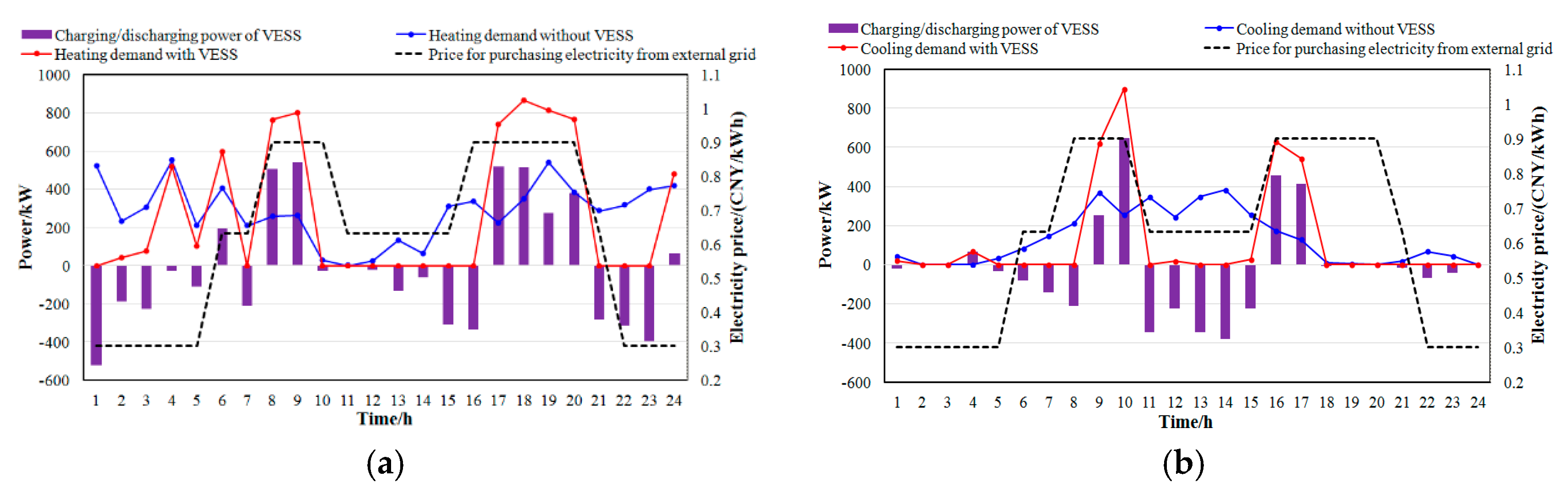
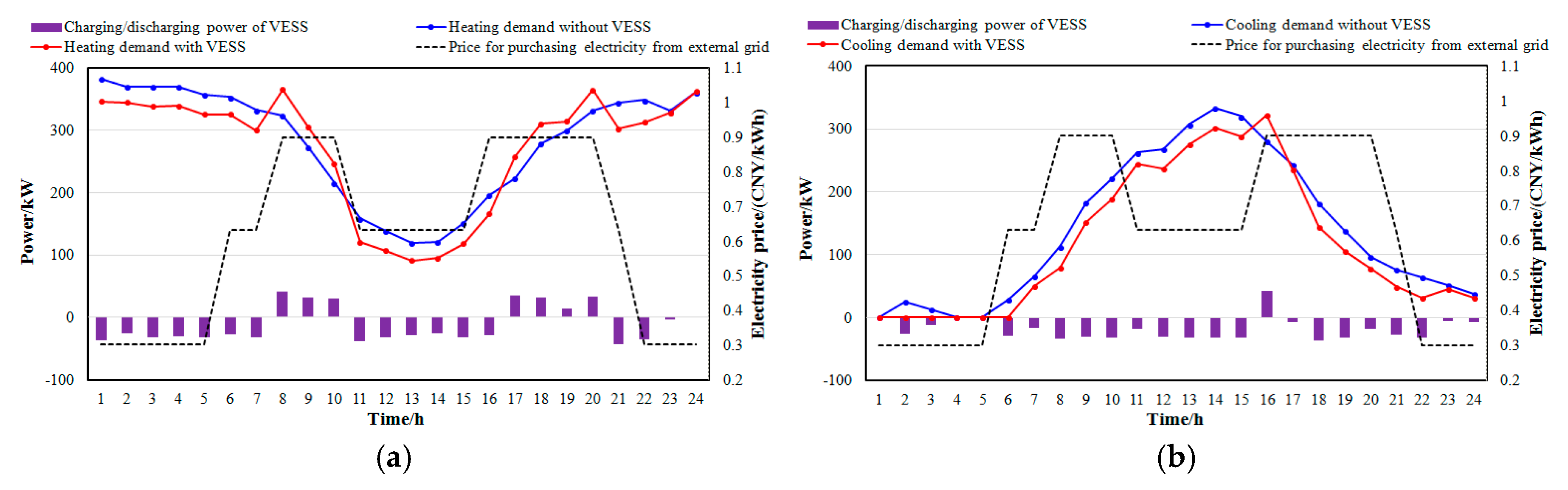
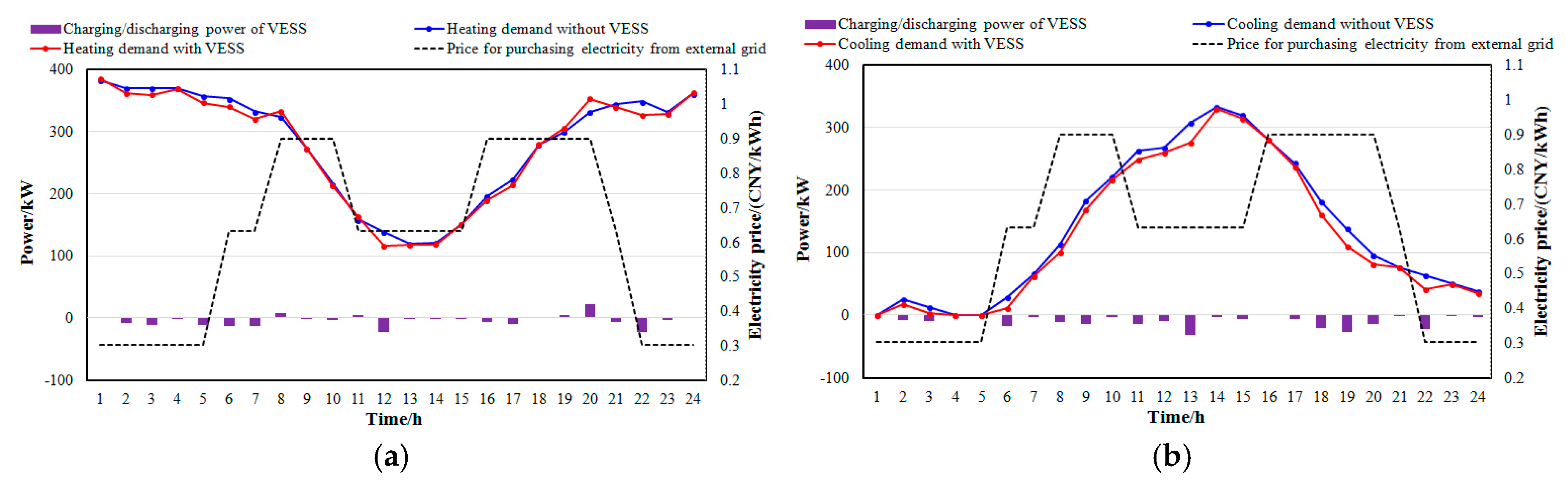
In this paper, heating/cooling demand of the RR-microgrid is the sum of the heating/cooling power generated by EHs/ECs and MTs. Treating the scheduling scheme for minimized TCL as the condition without VESS, while the best scheduling scheme and scheduling scheme for minimized OC as the condition with the VESS, respectively, then the curves of the heating/cooling demand with/without the VESS are shown in Figure 9 and Figure 10. Considering the curve of the heating/cooling demand without the VESS as the reference curve, it is known that the curve of the heating/cooling demand with the VESS fluctuates around the reference curve. Therefore, the part above the reference curve could be considered as ‘charging’, and the part below the reference curve could be considered as ‘discharging’, then charging/discharging power for the VESS is obtained as the difference of the heating/cooling demand between the two cases. It is found that the performance of the VESS in best scheduling scheme is quite similar with that in scheduling scheme for minimized OC for both the typical days. In addition, compared with BESS, the VESS has the contrary charging/discharging response to the changing of electricity price. For both typical days in winter/summer, the charging process of the VESS mainly happens during higher price periods, while the discharging process of the VESS mainly happens at lower price or middle-price periods.

Owing to the VESS capacity of RFHCS being quite considerable, the OC of the best scheduling scheme and the scheduling scheme for minimized OC has a dramatic decline compared with the condition without the VESS (55.90% and 64.98% for the typical day in winter, 73.99% and 75.68% for the typical day in summer).

6.2.2. Scheduling Results of the RR-Microgrid with CHCS

The Pareto-optimal front of the presented multi-objective optimization model obtained by the NSGA-II algorithm is shown in Figure 11. Similarly, it can be known that the NSGA-II algorithm could also gain enough optimal scheduling solutions.

The normalized objectives of Pareto-optimal front sorted by TCL are shown in Figure 12, obviously, and the OC and PE are also two opposite objectives where increasing one of them decreases the other one when TCL is invariable.

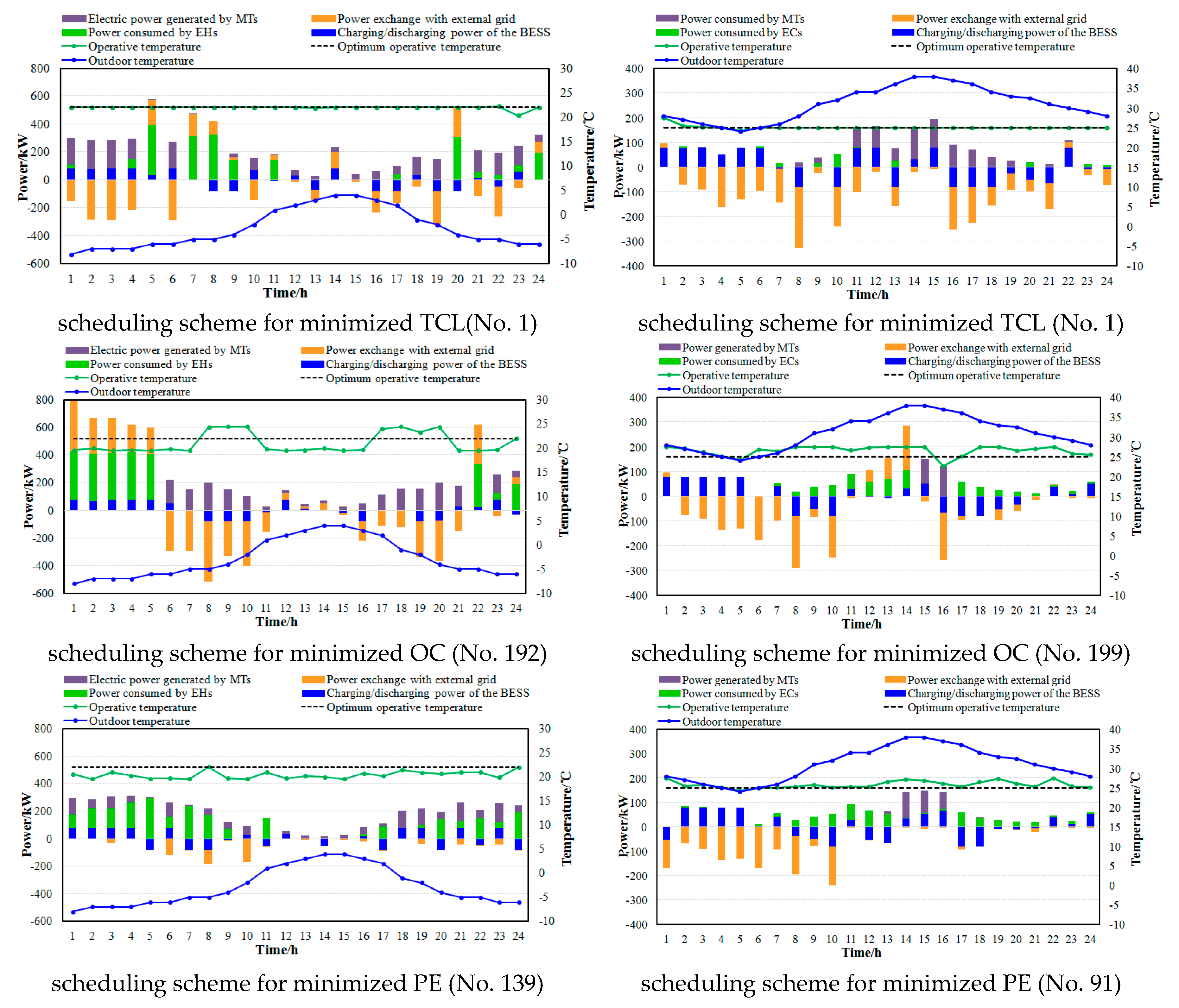
The optimal scheduling schemes for minimized TCL, OC, PE, as well as the best scheduling scheme determined by the AHP method are shown in Figure 13, and the corresponding objectives are shown in

Table 13. Value of objective functions of different scheduling schemes for a typical day in winter.

Objective Functions	OC (CNY)	TCL (°C2)	PE (kg)
No.1	2733.71	2.88	726.57
No.192	1686.66	123.22	957.37
No.139	2512.08	73.61	292.81
No.27	1911.02	15.24	518.05

and

Table 14. Value of objective functions of different scheduling schemes for a typical day in summer.

Objective Functions	OC (CNY)	TCL (°C2)	PE (kg)
No.1	840.75	0.73	166.17
No.199	545.72	85.99	154.49
No.91	689.18	28.64	57.64
No.77	604.29	22.72	84.35

. For the sake of convenience of representation, the discharging power of the BESS, as well as the electric power selling to the external grid, are also taken as negative in Figure 13.

For all of the above scheduling schemes, the charging/discharging behavior of the BESS are quite similar with that in the mentioned scheduling schemes for the RR-microgrid with RFHCS, that is to say, the charging behavior of the BESS prefers to happen during lower price periods, while the discharging behavior prefers to happen during higher price periods. However, the electric power consumed by EHs/ECs and generated by MTs are more balanced than the corresponding result in the RR-microgrid with RFHCS. The reason for this phenomenon is that the total heat capacity of the indoor air is quite smaller than that of the radiant floor, the heat/cool energy stored by the previous scheduling period is not enough to support the EHs/ECs and MTs to stop working for the next one or more scheduling periods.

As for the scheduling scheme for minimized TCL, the operative temperature is quite close to the optimum operative temperature at all of the scheduling periods, which also indicates that the thermal power generated by MTs and EHs/ECs could satisfy the heating/cooling demand quite well.

As for the scheduling scheme for minimized OC, on the typical day in winter, EHs only consume power during lower price periods, while the MTs mainly work during higher price periods; on the typical day in summer, MTs and ECs mainly work during the daytime for the cooling demand in the nighttime is quite small. The ECs consume power during most scheduling periods, while the MTs only work during the few higher outdoor temperature periods (14:00–16:00) when the cooling demand is greater to achieve better economy than ECs. On the typical day in winter, the operative temperature maintains at a low level during lower price periods while maintains at a high level during higher price periods. On the typical day in summer, the operative temperature maintains at a high level at most scheduling periods while maintaining at a low level during the few lower outdoor temperature periods (4:00–6:00) or the higher outdoor temperature periods (14:00–16:00). To achieve the minimized OC, on the typical day in winter, purchasing electric power from the external grid happens during lower-periods and selling electric power to the external grid happens during higher price periods; on the typical day in summer, purchasing electric power from the external grid happens mainly at midday scheduling periods while selling electric power to the external grid happens during most scheduling periods.

As for the scheduling scheme for minimized PE, for both typical days, there is also no electric power purchasing from the external grid due to the coal consumption has bigger total emission coefficient than natural gas. On the typical day in winter, the electric power selling to the external grid is obviously less than that of the scheduling schemes for minimized OC and TCL. While on the typical day in summer, the electric power selling to the external grid concentrate on the lower outdoor temperature periods (0:00–10:00) due to the cooling demand at that time is small.

As for the best scheduling scheme determined by the AHP method, compared with the scheduling the scheme for minimized OC, the operative temperature has a similar variation trend and has an obviously smaller variation magnitude so that TCL is dramatically decreased. Meanwhile, PE is effectively decreased.

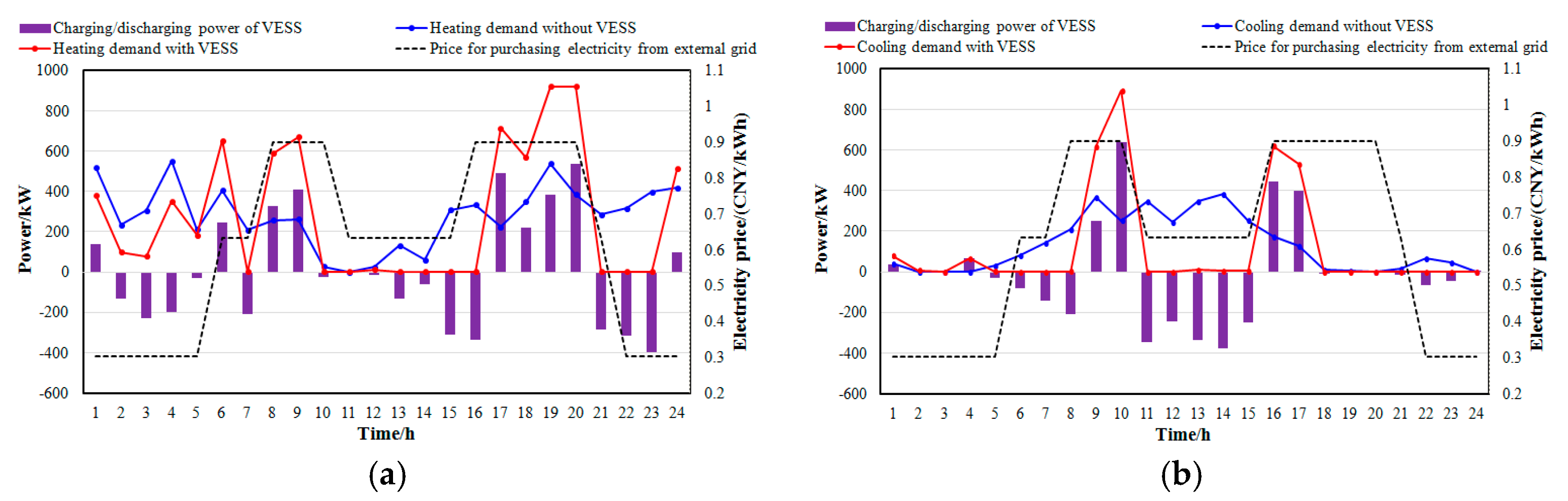
Similarly, we treat the scheduling scheme for minimized TCL as the condition without the VESS, while the best scheduling scheme and scheduling scheme for the minimized OC as the condition with the VESS, respectively; then the curves of heating/cooling demand with/without the VESS are shown in Figure 14 and Figure 15. For both the best scheduling scheme and scheduling scheme for the minimized OC, on the typical day in winter, the charging process of the VESS mainly happens during the higher price periods, while discharging process of the VESS mainly happens during the lower price periods; on the typical day in summer, the charging process of the VESS rarely happens while the discharging process of the VESS happens during most scheduling periods. Compared with the result shown in Figure 9 and Figure 10, it is found that the magnitude of the charging/discharging power of the VESS becomes significantly smaller. The reason for this phenomenon is that the VESS capacity of the CHCS is obviously smaller than that of the RFHCS. Consequently, compared with the condition without the VESS, the OC of the best scheduling scheme and scheduling scheme for the minimized OC has a relatively small decline (30.10% and 38.32% for a typical day in winter, 28.12% and 35.14% for a typical day in summer).

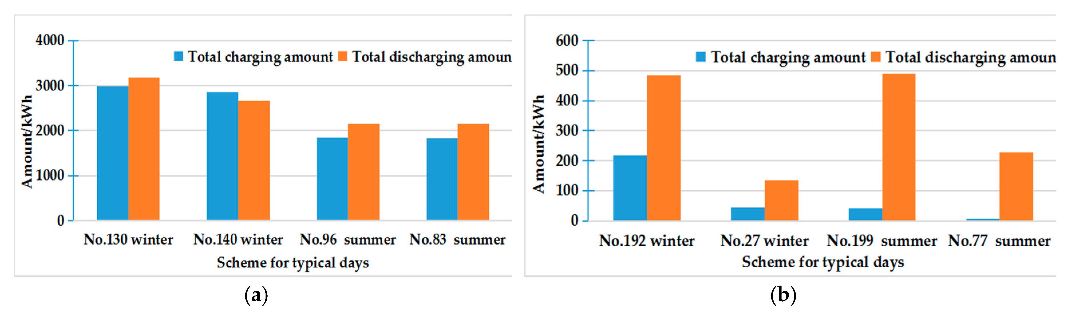
The charge/discharge power characteristics of the two kinds of VESS in the minimized OC scheduling scheme and in the best scheduling scheme are calculated, as shown in

Table 15. Performance of the VESS of RFHCS for the typical days in winter/summer.

Scheduling Scheme		Maximum Charging Power	Maximum Discharging Power	Mean Charging/Discharging Power	Total Charging Amount	Total Discharging Amount
Typical day in winter	No. 130	539.21	520.65	256.67	2989.17	3170.86
	No. 140	537.40	398.18	230.01	2851.14	2668.95
Typical day in summer	No. 96	647.90	382.67	166.20	1841.12	2158.66
	No. 83	638.87	379.26	166.66	1835.24	2153.42

,

Table 16. Performance of the VESS of CHCS for the typical days in winter/summer.

Scheduling Scheme		Maximum Charging Power	Maximum Discharging Power	Mean Charging/Discharging Power	Total Charging Amount	Total Discharging Amount
Typical day in winter	No. 192	41.38	42.59	29.26	217.39	484.88
	No. 27	21.55	22.29	7.44	42.96	135.66
Typical day in summer	No. 199	41.70	36.93	22.10	41.69	488.79
	No. 77	0.58	31.58	9.54	0.58	228.34

, and Figure 16. It can be known that, compared with the VESS of CHCS, the charge/discharge power characteristics of the VESS of the RFHCS in the minimized OC scheduling scheme are more similar with that in the best scheduling scheme. In addition, the mean charging/discharging power and the total charging/discharging amount are obviously greater, indicating that the heat capacity of the heavy radiant floor is much higher than that of the indoor air.

7. Conclusions

A novel multi-objective optimal scheduling method for a grid-connected RR-microgrid is presented in which the heating/cooling system of a residential building is considered as a virtual energy storage system. The following conclusions are drawn:

(1)

The NSGA-II algorithm could obtain enough optimal scheduling schemes for the presented multi-objective optimization model of RR-microgrid, and the OC and PE are two opposite objectives where increasing one of them decreases the other one when TCL is invariable. The best scheduling scheme could be reasonably selected by the AHP method according to the set of weights of each objective.

(2)

As for the best scheduling scheme of RR-microgrid with RFHCS, the charging process of VESS mainly happens during higher price periods, while the discharging process of VESS mainly happens during lower price or middle price periods for both typical days in winter/summer.

(3)

As for the best scheduling scheme of the RR-microgrid with CHCS, on the typical day in the winter, the charging process of the VESS mainly happens during higher electricity price periods, and the discharging process of the VESS mainly happens during lower electricity price periods; on a typical day in the summer, the charging process of VESS rarely happens while the discharging process of VESS happens during most scheduling periods.

(4)

Due to the VESS capacity of the CHCS being obviously smaller than that of the RFHCS, as for the corresponding best scheduling scheme, the electric power consumed by EHs/ECs and generated by MTs in the RR-microgrid with CHCS are more balanced than that in the R-microgrid with RFHCS. Meanwhile, compared with the condition without VESS, the OC of the RR-microgrid with RFHCS has a greater decline than that of the RR-microgrid with CHCS.

References

- European Commission. A Policy Framework for Climate and Energy in the Period from 2020 up to 2030, Brussels. 2014. Available online: http://eur-lex.europa.eu/legal-content/EN/TXT/?uri=CELEX:52013DC0169 (accessed on 17 May 2019).
- den Elzen, M.; Fekete, H.; Höhne, N.; Admiraal, A.; Forsell, N.; Hof, A.F.; Olivier, J.G.; van Soest, H. Greenhouse gas emissions from current and enhanced policies of China until 2030: Can emissions peak before 2030? Energy Policy 2016, 89, 224–236. [Google Scholar] [CrossRef]
- Yang, L.; Wang, J.; Shi, J. Can China meet its 2020 economic growth and carbon emissions reduction targets? J. Clean. Prod. 2017, 142, 993–1001. [Google Scholar] [CrossRef]
- Jin, X.; Wu, J.; Mu, Y.; Wang, M.; Xu, X.; Jia, H. Hierarchical microgrid energy management in an office building. Appl. Energy 2017, 208, 480–494. [Google Scholar] [CrossRef]
- Yu, J.; Tian, L.; Xu, X.; Wang, J. Evaluation on energy and thermal performance for office building envelope in different climate zones of China. Energy Build. 2015, 86, 626–639. [Google Scholar] [CrossRef]
- Guan, X.; Xu, Z.; Jia, Q. Energy-efficient buildings facilitated by microgrid. IEEE Trans. Smart Grid 2010, 1, 243–252. [Google Scholar]
- Pesin Michael. U.S. Department of Energy Electricity Grid Research and Development. In Proceedings of the American Council of Engineering Companies, Environment and Energy Committee Winter Meeting, Washington, DC, USA, 9 February 2017. [Google Scholar]
- Navigant Research. More Than 400 Microgrid Projects are Under Development Worldwide [EB/OL]. Available online: http://www.navigantresearch.com/newsroom/more-than-400-microgrid-projects-are-under-development-worldwide (accessed on 2 April 2013).
- Feng, W.; Jin, M.; Liu, X.; Bao, Y.; Marnay, C.; Yao, C.; Yu, J. A review of microgrid development in the United States–A decade of progress on policies, demonstrations, controls, and software tools. Appl. Energy 2018, 228, 1656–1668. [Google Scholar] [CrossRef]
- Cagnano, A.; De Tuglie, E.; Cicognani, L. Prince-Electrical Energy Systems Lab: A pilot project for smart microgrids. Electr. Power Syst. Res. 2017, 148, 10–17. [Google Scholar] [CrossRef]
- Jaramillo, L.B.; Weidlich, A. Optimal microgrid scheduling with peak load reduction involving an electrolyzer and flexible loads. Appl. Energy 2016, 169, 857–865. [Google Scholar] [CrossRef]
- Wu, X.; Wang, X.; Wang, J.; Bie, C. Economic generation scheduling of a microgrid using mixed integer programming. Proc. CSEE 2013, 33, 1–8. (In Chinese) [Google Scholar]
- Jiang, Q.; Xue, M.; Geng, G. Energy management of microgrid in grid-connected and stand-alone modes. IEEE Trans. Power Syst. 2013, 28, 3380–3389. [Google Scholar] [CrossRef]
- Lu, Y.; Wang, S.; Sun, Y.; Yan, C. Optimal scheduling of buildings with energy generation and thermal energy storage under dynamic electricity pricing using mixed-integer nonlinear programming. Appl. Energy 2015, 147, 49–58. [Google Scholar] [CrossRef]
- Zhao, Y.; Lu, Y.; Yan, C.; Wang, S. MPC-based optimal scheduling of grid-connected low energy buildings with thermal energy storages. Energy Build. 2015, 86, 415–426. [Google Scholar] [CrossRef]
- Javidsharifi, M.; Niknam, T.; Aghaei, J.; Mokryani, G. Multi-objective short-term scheduling of a renewable-based microgrid in the presence of tidal resources and storage devices. Appl. Energy 2018, 216, 367–381. [Google Scholar] [CrossRef]
- Carpinelli, G.; Mottola, F.; Proto, D.; Russo, A. A multi-objective approach for microgrid scheduling. IEEE Trans. Smart Grid 2017, 8, 2109–2118. [Google Scholar] [CrossRef]
- Lin, W.; Jin, X.; Mu, Y.; Jia, H.; Xu, X.; Yu, X.; Zhao, B. A two-stage multi-objective scheduling method for integrated community energy system. Appl. Energy 2018, 216, 428–441. [Google Scholar] [CrossRef]
- Yin, Z.; Che, Y.; Li, D.; Liu, H.; Yu, D. Optimal scheduling strategy for domestic electric water heaters based on the temperature state priority list. Energies 2017, 10, 1425. [Google Scholar] [CrossRef]
- Lu, N. An evaluation of the HVAC load potential for providing load balancing service. IEEE Trans. Smart Grid 2012, 3, 1263–1270. [Google Scholar] [CrossRef]
- Wang, C.; Liu, M.; Lu, N. A tie-line power smoothing method for microgrid using residential thermostatically-controlled loads. Proc. CSEE 2012, 2, 36–43. (In Chinese) [Google Scholar]
- Jia, H.; Qi, Y.; Mu, Y. Frequency response of autonomous microgrid based on family-friendly controllable loads. Sci. China Technol. Sci. 2013, 43, 247–256. (In Chinese) [Google Scholar] [CrossRef]
- Van, R.J.; Leemput, N.; Geth, F.; Büscher, J.; Salenbien, R.; Driesen, J. Electric vehicle charging in an office building microgrid with distributed energy resources. IEEE Trans. Sustain. Energy 2014, 5, 1–8. [Google Scholar] [CrossRef]
- Igualada, L.; Corchero, C.; Cruz-Zambrano, M.; Heredia, F.J. Optimal energy management for a residential microgrid including a vehicle-to-grid system. IEEE Trans. Smart Grid 2014, 5, 2163–2172. [Google Scholar] [CrossRef]
- Jin, X.; Mu, Y.; Jia, H. Optimal scheduling method for a combined cooling, heating and power building microgrid considering virtual storage system at demand side. Proc. CSEE 2017, 37, 581–590. (In Chinese) [Google Scholar]
- Jin, X.; Mu, Y.; Jia, H.; Wu, J.; Tao, J.; Yu, X. Dynamic economic dispatch of a hybrid energy microgrid considering building based virtual energy storage system. Appl. Energy 2016, 194, 386–398. [Google Scholar] [CrossRef]
- Liu, W.; Liu, C.; Lin, Y.; Ma, L.; Bai, K.; Wu, Y. Optimal scheduling of residential microgrids considering virtual energy storage system. Energies 2018, 11, 942. [Google Scholar] [CrossRef]
- Fanger, P.O. Analysis and Applications in Environmental Engineering; Thermal Comfort Analysis & Applications in Environmental Engineering; McGraw Hill: New York, NY, USA, 1970. [Google Scholar]
- Wang, J. Optimal Design of Building Cooling Heating and Power System and Its Multi-Criteria Integrated Evaluation Method. Ph.D. Thesis, North China Electric Power University, Beijing, China, 2010. [Google Scholar]
- Brownlee, A.E.I.; Wright, J.A. Constrained, mixed-integer and multi-objective optimisation of building designs by NSGA-II with fitness approximation. Appl. Soft Comput. 2015, 33, 114–126. [Google Scholar] [CrossRef]
- Deb, K.; Pratap, A.; Agarwal, S.; Meyarivan, T. A fast and elitist multiobjective genetic algorithm: NSGA-II. IEEE Trans. Evol. Comput. 2002, 6, 182–197. [Google Scholar] [CrossRef]
- Chen, W. Quantitative decision-making model for distribution system restoration. IEEE Trans. Power Syst. 2010, 25, 313–321. [Google Scholar] [CrossRef]
- Zhao, K.; Liu, X.; Jiang, Y. Dynamic performance of water-based radiant floors during start-up and high-intensity solar radiation. Sol. Energy 2014, 101, 232–244. [Google Scholar] [CrossRef]
Figure 1.
Structure of the studied RR-microgrid.
Figure 2.
ETP models for different heating/cooling systems. (a) RFHCS; and (b) CHCS.
Figure 3.
Flowchart of the NSGA-II algorithm.
Figure 4.
Forecasted curves of solar radiation intensity and outdoor temperature.
Figure 5.
Forecasted curves of WT output, PV output, electric load, and electricity price curve.
Figure 6.
Pareto front of optimal scheduling for RR-microgrid with RFHCS. (a) A typical day in winter; and (b) a typical day in summer.
Figure 7.
The normalized objectives of Pareto front of optimal scheduling for RR-microgrid with RFHCS. (a) A typical day in winter; and (b) a typical day in summer.
Figure 8.
The optimal scheduling results for RR-microgrid with RFHCS. (a) A typical day in winter; and (b) a typical day in summer.
Figure 9.
VESS charging/discharging power in minimized OC scheduling scheme for RR-microgrid with RFHCS. (a) A typical day in winter; and (b) a typical day in summer.
Figure 10.
VESS charging/discharging power in best scheduling scheme for RR-microgrid with RFHCS. (a) A typical day in winter; and (b) a typical day in summer.
Figure 11.
Pareto front of optimal scheduling for RR-microgrid with CHCS. (a) A typical day in winter; and (b) a typical day in summer.
Figure 12.
The normalized objectives of Pareto front of optimal scheduling for the RR-microgrid with CHCS. (a) A typical day in winter; and (b) a typical day in summer.
Figure 13.
The optimal scheduling results for RR-microgrid with CHCS. (a) A typical day in winter; and (b) a typical day in summer.
Figure 14.
VESS charging/discharging power in minimized OC scheduling scheme for RR-microgrid with CHCS. (a) A typical day in winter; and (b) a typical day in summer.
Figure 15.
VESS charging/discharging power in best scheduling scheme for RR-microgrid with CHCS. (a) A typical day in winter; and (b) a typical day in summer.
Figure 16.
Comparison of total charging/discharging amount. (a) VESS of RFHCS; and (b) VESS of CHCS.