Identifiability and Reconstruction of Biochemical Reaction Networks from Population Snapshot Data

Abstract

Inference of biochemical network models from experimental data is a crucial problem in systems and synthetic biology that includes parameter calibration but also identification of unknown interactions. Stochastic modelling from single-cell data is known to improve identifiability of reaction network parameters for specific systems. However, general results are lacking, and the advantage over deterministic, population-average approaches has not been explored for network reconstruction. In this work, we study identifiability and propose new reconstruction methods for biochemical interaction networks. Focusing on population-snapshot data and networks with reaction rates affine in the state, for parameter estimation, we derive general methods to test structural identifiability and demonstrate them in connection with practical identifiability for a reporter gene in silico case study. In the same framework, we next develop a two-step approach to the reconstruction of unknown networks of interactions. We apply it to compare the achievable network reconstruction performance in a deterministic and a stochastic setting, showing the advantage of the latter, and demonstrate it on population-snapshot data from a simulated example.

1. Introduction

A central problem in systems and synthetic biology is the calibration of the unknown parameters of a biochemical reaction network model on the basis of real data [1]. Sometimes, the network of interactions in the system of interest is not completely known and needs to be reconstructed from data as well [2]. In synthetic biology, this is of special interest since the engineering of circuits into cells may result in unexpected interactions [3]. For parameter inference, a central question is what parameters of a given model can be identified unambiguously by a given experimental setup. This is the problem of identifiability, which is dedicated much attention in the systems’ biology literature since crucial for the correct interpretation of inference results [4,5,6]. Posed purely in terms of model properties, the question goes under the name of structural identifiability. When instead the quality of the data is also taken into account, attention shifts to estimation accuracy and leads to the concept of practical identifiability. With an appropriate reformulation, similar questions can be addressed for the reconstruction of interaction networks.

Model experimental technologies in cellular biology allow one to measure reaction dynamics with single-cell resolution [7]. Correspondingly, stochastic reaction network models are utilized to explain variability of reaction dynamics, notably gene expression, across cells. It has been realized that the combination of stochastic modelling and single-cell measurements allows one to discriminate parameters of reaction models that would not be identifiable based on deterministic modelling counterparts and population-averaged data [8,9,10]. While demonstrated on specific case studies, this point has not been addressed in much generality. At the same time, one expects that the advantage of stochastic modelling and single-cell measurements for parameter identifiability carries over to the problem of network inference. Whereas network inference has received attention in a deterministic context [11,12], the problem has barely been addressed in a stochastic setting, and a comparative study of network identifiability in the two settings does not exist.

In this paper, we discuss identifiability and reconstruction of unknown parameters and interactions in biochemical reaction networks. We focus on the fundamental class of models with reaction rates that are affine functions of the network state, and look at inference problems from mean and covariance time-profiles of the network state, as obtained from population-snapshot measurements [13]. State-affine rates reflect networks composed of reactions of zeroth or first order. Such networks occur naturally in gene expression modelling [14] and constitute the starting point to investigate more complex networks [15]. Population snapshot data, on the other hand, is easily obtained e.g., by inexpensive cytometry measurements, but is also the most immediate outcome of videomicroscopy [7]. Thus, we work in a framework that is at the same time sufficiently flexible and amenable of in-depth analysis via, in particular, the moment equations [16,17]. This allows us to establish the following tools and results.

For the parameter estimation problem, we develop general results and inexpensive methods to test structural identifiability, and discuss connections with practical identifiability. In the case of a random telegraph model of gene expression [14], we apply our methods to extend existing identifiability results [8,10] and discuss practical identifiability on the basis of numerical simulations. For the reconstruction of interaction networks, we develop a two-step method where a first step devoted to the identification of the network moment dynamics is followed by a second step that determines the network of interactions by the algorithmic solution of a factorization problem. We notably compare the deterministic (population-average) and stochastic (single-cell) scenarios, demonstrating the superiority of the latter from a theoretical viewpoint and also numerically on a toy example.

This work is an extension and consolidation of earlier results by the same author and published as part of conference proceedings in [18] (parameter identifiability) and [19] (network reconstruction). Relevant work on parameter identifiability in the context of biochemical networks has been developed by several authors (see [4,6,8,20] and references therein). Relative to the state of the art, our results on structural identifiability are entirely novel, while the discussion of practical identifiability is in the same spirit as e.g., [1]. Reconstruction of biochemical networks is reviewed in [11,12,21,22] (see also [23]) and is even dedicated a yearly challenge boosting continuous investigation (see [2]). However, from the viewpoint of stochastic dynamics and single-cell data, existing contributions are essentially limited to model discrimination and selection among small pools of specific network alternatives (see, e.g., [24]). Moreover, to our knowledge, a comparative analysis of network identifiability in the deterministic and stochastic setups is not present in literature. Our work contributes to fill this gap with an original analysis and methods for the reconstruction of stochastic biochemical interaction networks with no a priori restriction on the network structure for a given set of species.

The paper is organized as follows. In Section 2, we review stochastic modelling of biochemical reaction networks. In particular, in Section 2.1, we derive an especially convenient form for the moment equations that will be the working tool for the rest of the work. Section 3 is devoted to parameter identifiability. In particular, our novel methods for structural identifiability are derived in Section 3.1. Together with the practical identification tools reviewed in Section 3.2, they are applied to the case of the random telegraph model for a reporter gene system in Section 3.3. Section 4 addresses network reconstruction. The theoretical analysis and development of the two steps (Section 4.1 and Section 4.2) of the reconstruction problem are turned into a novel practical network identification procedure in Section 4.3. Analysis and reconstruction methods are then demonstrated on a toy network in Section 4.4. Final discussion is presented in Section 5. For mathematical formulas, we stick to common notation, adding explanations where needed.

2. Modelling of Biochemical Reaction Networks

A reaction network is a family of $n\in \mathbb{N}$ chemical species ${\mathcal{S}}_1,\dots ,{\mathcal{S}}_n$ and $m\in \mathbb{N}$ reactions ${\mathcal{R}}_1,\dots ,{\mathcal{R}}_m$ that may occur among them in a given reaction volume. The stoichiometry matrix of the network, $S=[S_1,\dots ,S_m]\in {\mathbb{Z}}^{n\times m}$, is defined such that the ith row of $S_j$ is the net change in the number of molecules of ${\mathcal{S}}_i$ when reaction ${\mathcal{R}}_j$ occurs, with $i=1,\dots ,n$ and $j=1,\dots ,m$. Let $X_i\left(t\right)$ be the number of molecules of ${\mathcal{S}}_i$ at time t, and $X\left(t\right)={[X_1\left(t\right)\cdots X_n\left(t\right)]}^T$. The evolution of $X\left(t\right)$ depends on the random occurrence of reactions ${\mathcal{R}}_j$, thus $X\left(t\right)$ is, in general, a random vector. Under suitable assumptions on the reaction volume and the physics of the reactions [25], one has that $X\left(t\right)$ follows the laws of a Continuous-Time Markov Chain (CTMC), with the columns of S as possible state transitions and transition probabilities

$$\begin{array}{cccc}\hfill \mathbb{P}\left[X\right(t+dt)& =x+S_j|X\left(t\right)=x]=a_j(x,t)dt+o\left(dt\right),\hfill & \hfill j& =1,\dots ,m.\hfill \end{array}$$

Reaction rates $a(x,t)={[a_1(x,t),\dots ,a_m(x,t)]}^T$ depend on the current abundance x of molecules of the different species, and possibly on time t e.g., in the presence of environmental perturbations. They entirely specify the time dynamics of $\mathbb{P}\left[X\right(t\left)\right]$ as expressed by the Chemical Master Equation [25].

We focus on reaction rates that are affine in the state, that is,

$$a(x,t)=Wx+w_0\left(t\right),$$

(1)

where $W\in {\mathbb{R}}^{m\times n}$ and $w_0\left(t\right):\mathbb{R}\to {\mathbb{R}}^m$ is piecewise continuous (W may as well depend on t, but we will not address this scenario here). This form is typical of networks comprising zeroth- and first-order reactions only, as dictated by the mass-action laws [26]. In cellular biology, affine rates arise naturally in the modelling of gene expression (see later Section 3.3), and constitute the starting point for the (possibly approximate) modelling and analysis of regulatory networks [15]. The choice of state-affine rates and possible generalizations are further discussed in Section 5.

Note that, together, the patterns of nonzero entries of S and W define the network of regulatory interactions among the different species (see also [27]). Indeed, for every reaction j, the jth row of W tells what species regulate the reaction rate, whereas the jth column of S tells what species are affected by that reaction. Thus, if $S_{i,j}\ne 0$ and $W_{j,k}\ne 0$ for some j, $X_k$ directly regulates the dynamics of $X_i$, whereas, if $S_{i,j}=0$ or $W_{j,k}=0$ for all j, $X_k$ does not exert a direct regulation of the dynamics of $X_i$.

Denote $\mu \left(t\right)=\mathbb{E}\left[X\right(t\left)\right]$ and $\Sigma \left(t\right)=\mathrm{Var}\left(X\left(t\right)\right)=\mathbb{E}\left[(X\left(t\right)-\mu \left(t\right)){(X\left(t\right)-\mu \left(t\right))}^T\right]$ (“$\mathbb{E}[·]$” indicates expectation). It can be shown that the time evolution of the mean vector $\mu$ and of the covariance matrix $\Sigma$ obeys the so-called Moment Equations [16],

$$\begin{array}{cc}\hfill \dot{\mu }\left(t\right)& =SW\mu \left(t\right)+S{w}_0\left(t\right),\hfill \end{array}$$

(2)

$$\begin{array}{cc}\hfill \dot{\Sigma }\left(t\right)& =SW\Sigma \left(t\right)+\Sigma \left(t\right)W^T{S}^T+S\mathrm{diag}\left(W\mu \left(t\right)+w_0\left(t\right)\right)S^T,\hfill \end{array}$$

(3)

with initial conditions $\mu \left(t_0\right)={\mu }_0$ and $\Sigma \left(t_0\right)={\Sigma }_0$ determined by the initial probability distribution of X at a time $t_0$ (we will conventionally fix this time to $t_0=0$). This is a set of linear equations in the entries of $\mu$ and $\Sigma$. Similar, though more intricate, equations could be written for higher-order moments [17], but we will not use them. Equation (2), describing the evolution of the process mean, also provides by definition the mean-field approximation of the system and, for networks with negligible random fluctuations, its deterministic dynamics. Equation (3) instead quantifies the strength of the stochastic fluctuations around the system mean. If rates are not in the form (1), the description of the moments and the mean-field approximation of the system dynamics are involved (see, e.g., [28,29]).

2.1. Vector Representation of Moment Equations

Thanks to linearity, Equations (2) and (3) can be rewritten in the form

$$\begin{array}{cccc}\hfill \dot{z}\left(t\right)& =Az\left(t\right)+B{w}_0\left(t\right),\hfill & \hfill t& \ge 0,\hfill \end{array}$$

(4)

where $z\left(t\right)$ is a vector formed by the entries of $\mu \left(t\right)$ and $\Sigma \left(t\right)$, whereas A and B are matrices of appropriate dimension fixed by S and W. This representation is non-unique as it depends in particular on the ordering of the entries of z. One such representation is the following. Let “$\mathrm{vec}(·)$” be the operation of stacking the columns of a matrix into a single column vector, and let “⊗” denote the Kronecker product.

Proposition 1.

Let $\underline{\Sigma }\triangleq \mathrm{vec}(\Sigma )\in {\mathbb{R}}^{n^2}$ and $S^{\left(2\right)}\triangleq \left[\begin{array}{ccc}\mathrm{vec}\left(S_1{S}_1^T\right)& \cdots & \mathrm{vec}\left(S_m{S}_m^T\right)\end{array}\right]$. Equation (4) holds with

$$\begin{array}{cccccc}\hfill z& =\left[\begin{array}{c}\mu \left(t\right)\\ \underline{\Sigma }\left(t\right)\end{array}\right],\hfill & \hfill A& =\left[\begin{array}{cc}SW& 0_{n\times n^2}\\ S^{\left(2\right)}W& I_n\otimes \left(SW\right)+\left(SW\right)\otimes I_n\end{array}\right],\hfill & \hfill B& =\left[\begin{array}{c}S\\ S^{\left(2\right)}\end{array}\right].\hfill \end{array}$$

(5)

Proof. 

We start by rewriting (3) in vector form. Let us drop index t from notation for brevity. By the properties of Kronecker product, one gets that

$$\dot{\underline{\Sigma }}=[I_n\otimes \left(SW\right)+\left(SW\right)\otimes I_n]·\underline{\Sigma }+\mathrm{vec}\left(S\mathrm{diag}(W\mu +w_0)S^T\right).$$

In order to write the rightmost term in a more convenient form, observe that

$$S\mathrm{diag}(W\mu +w_0)S^T=\sum _{j=1}^{n}S\mathrm{diag}\left(W_j\right)S^T{\mu }_j+S\mathrm{diag}\left(w_0\right)S^T,$$

where $W_j$ denotes the j-th column of W. Therefore,

$$\mathrm{vec}\left(S\mathrm{diag}(W\mu +w_0)S^T\right)=\left[\begin{array}{c}\mathrm{vec}\left(S\mathrm{diag}\left(W_1\right)S^T\right),\dots ,\mathrm{vec}\left(S\mathrm{diag}\left(W_n\right)S^T\right)\end{array}\right]·\mu +\mathrm{vec}\left(S\mathrm{diag}\left(w_0\right)S^T\right).$$

Next note that, for any vector w of appropriate size, $\mathrm{vec}\left(S\mathrm{diag}\left(w\right)S^T\right)=S^{\left(2\right)}w$. Then, we may write

$$\dot{\underline{\Sigma }}=[I_n\otimes \left(SW\right)+\left(SW\right)\otimes I_n]·\underline{\Sigma }+S^{\left(2\right)}W·\mu +S^{\left(2\right)}·w_0.$$

Together with Equation (2), this yields the result. □

In the sequel, we let (5) be the definition of z, A and B. Note that this representation is redundant, since the upper- and lower-triangular part of the symmetric matrix $\Sigma$ are both included in z. In addition, depending on the definition of process $X\left(t\right)$, relationships among the entries $\mu$ and $\Sigma$ may further reduce the effective dimensionality of the system [30].

2.2. Input–Output Model

For identification purposes, well-defined time-varying stimuli are usually applied to a biochemical network to explore its dynamics. These perturbation inputs typically enter the system in a way that is known only in part. Here, we focus on the scenario where the inputs act on rates $w_0\left(t\right)$. A natural manner to express the dependency of $w_0\left(t\right)$ on known inputs $u\left(t\right)$ is to write

$$w_0\left(t\right)=Gu\left(t\right),$$

(6)

where G is an $m\times n_u$ matrix of (possibly null) constants, while $u\left(t\right)$ is an $n_u$-dimensional vector of (possibly constant) functions. In general, we let $u(·)$ belong to the space of piecewise-continuous (vector) functions $\mathcal{U}$. In the sequel, we will consider $u(·)$ to be known and treat G as possibly unknown parameters, reflecting partially unknown effects of inputs of reaction rates.

A chief biological application of stochastic reaction networks is to describe variability of the individual cell dynamics in an isogenic population. In this context, the different random outcomes of $X\left(t\right)$ correspond to different dynamics of individual cells in the same environment. Accordingly, Equations (2) and (3) describe how the statistics of $X\left(t\right)$ over the cell population evolve over time. Depending on the biochemical system under consideration, several experimental techniques are available to monitor the evolution of these statistics, ranging from population-average to individual-cell measurements. From the mathematical viewpoint, they differ in the order of the moments and in the state variables that are monitored. As far as moments up to second order are concerned, we may describe the observed moments as

$$y(·)=C·z(·),$$

(7)

where C is a matrix of size $n_y\times (n+n^2)$ and z obeys Equation (4). Typically C is a $(0,1)$-matrix that selects the observed entries of z, so that $n_y$ is simply the number of observed moments. For a sequence of $N_y$ measurement times $t_{\ell }$, with $\ell =1,\dots ,N_y$, we may then define the experimental measurements of y as

$$\begin{array}{cccc}\hfill {\tilde{y}}_{\ell }& =y\left(t_{\ell }\right)+e_{\ell },\hfill & \hfill \ell & =1,\dots ,N_y,\hfill \end{array}$$

(8)

where $e_{\ell }$ accounts for measurement error.

For population-average measurements, C only selects the entries of y from those of $\mu$. Note that the selected entries of $\mu$, corresponding to different species ${\mathcal{S}}_i$, can be observed in separate experiments, as long as the moment equations (that is, the network state statistics) are the same across all experiments. For individual-cell measurements obtained e.g., by flow-cytometry, C most often selects the entries of $\mu$ and $\mathrm{diag}(\Sigma )$ in accordance with the monitored species ${\mathcal{S}}_i$. Again, several species monitored in different experiments are accounted for at once by Equation (8) as long as z obeys the same moment equations across all experiments. A definition of C such that non-diagonal entries ${\Sigma }_{i,i^{\prime }}$ of $\Sigma$ enter vector y instead subsumes experiments where species ${\mathcal{S}}_i$ and ${\mathcal{S}}_{i^{\prime }}$ are quantified simultaneously in individual cells (covariance of $X_i$ and $X_{i^{\prime }}$ cannot be determined from independent experiments separately targeting i and $i^{\prime }$). In general, for the later mathematical developments, C can be any real matrix of appropriate size. Finally, the statistical model for the error terms $e_{\ell }$ depends on the experimental technique. We will not discuss different possible error models here. Where needed in the sequel, following a common practice, we will assume the $e_{\ell }$ to be mutually independent Gaussian random vectors,

$$\begin{array}{cccc}\hfill e_{\ell }& \sim \mathcal{N}(0,R_{\ell }^2),\hfill & \hfill \hspace{1em}\hspace{1em}\hspace{1em}\hspace{1em}\hspace{1em}\hspace{1em}\hspace{1em}\mathbb{E}\left[e_{\ell }{e}_{{\ell }^{\prime }}\right]& =0,\ell \ne {\ell }^{\prime },\hfill \end{array}$$

(9)

with the $R_{\ell }^2$ known (or estimated from the data). In connection with the discussion above, this model is notably advocated in [9] for flow-cytometry measurements.

In view of the above definitions, in vector form, the moment equation system relating inputs u to the observed outputs y is

$$\begin{array}{cc}\hfill \dot{z}\left(t\right)& =Az\left(t\right)+BGu\left(t\right),\hfill \end{array}$$

(10)

$$\begin{array}{cc}\hfill y\left(t\right)& =Cz\left(t\right),\hfill \end{array}$$

(11)

with z, A and B as in Equation (5), and time-sampled, noisy measurements of y as in Equations (8) and (9).

3. Identification of Parameters

Assuming S and C known, in this section, we consider the problem of estimating the reaction rate parameters W and G that define the model of Equations (10) and (11) via (5) from experimental data (8) and (9). Since ${\mu }_0$ and ${\Sigma }_0$ are also unknown in most practical scenarios, we let $z_0=z\left(0\right)$ be an additional parameter vector to be estimated. We assume that $u\left(t\right)$ is a known input vector of the reaction network, such as controlled environmental stimuli. The choice of appropriate inputs and observables, i.e., function $u(·)$ and matrix C, in an experiment design phase is an intriguing and important subject, but its full treatment is beyond the scope of this paper. We will limit ourselves to commenting on this point when relevant.

In general, some entries of W, G and $z_0$, such as null entries for species that do not participate in certain reactions or that are initially absent, may be known in advance. At the same time, as in the example of Section 3.3 later on, some of the unknown entries of W, G and $z_0$ may be identical by construction. Taking this into account, let $\theta ={[{\theta }_1,\dots ,{\theta }_N]}^T$ be the vector of unknown, distinguished entries of W, G, and $z_0$, in some convenient order. We assume that $\theta \in \Theta$, where $\Theta \subseteq {\mathbb{R}}^N$ is given. To avoid technical complicacies, we let $\Theta$ be nonempty and open, and elaborate on this hypothesis when appropriate.

The first question to be addressed is whether the values of $\theta$ can be uniquely resolved based on the system observables, regardless of the quality and frequency of the measurements. This is the problem of structural identifiability, which concerns properties of the system model and its observables. In our context, given model (10)–(11), it addresses the question whether the relationship between $\theta$ and $y(·)$ is one-to-one. Structural identifiability is treated in Section 3.1.

The second question is the accuracy by which the model parameters can be estimated from actual data. This is the problem of practical identifiability. In addition to the model properties, it also concerns the quality and frequency of the data, as defined by Equation (8), and the properties of the measurement error. Intuitively, this question is only well-posed for systems that are structurally identifiable. However a formal definition of practical identifiability is not obvious and still open (see [1,4,6,20], among others). Rather than a theoretical discussion of practical identifiability, we will briefly review the Maximum Likelihood (ML) approach to identification from noisy data and related performance evaluation tools in Section 3.2, and discuss practical identifiability results in relation with estimation performance and structural identifiability on a numerical case study in Section 3.3.

3.1. Structural Identifiability

In this section, we review the formal notion of structural identifiability and develop novel methods to test structural identifiability for networks with affine rates. For any given $\theta \in \Theta$, let ${\widehat{y}}_{\theta }$ be the corresponding solution ${y\left(t\right)|}_{t\ge 0}$ of Equations (10) and (11), and let

$$\mathcal{M}(\Theta )=\{{\widehat{y}}_{\theta }:\theta \in \Theta \}.$$

(12)

Structural identifiability is then a property of the model family (12), as expressed via the following classical definitions [31].

Definition 1 (Identifiability at a point).

The model family (12) is

(a) 

locally identifiable at${\theta }^{\ast }\in \Theta$if, for some neighborhood$B_{{\theta }^{\ast }}\subseteq \Theta$of${\theta }^{\ast }$,

$${\widehat{y}}_{\theta }={\widehat{y}}_{{\theta }^{\ast }}\Rightarrow \theta ={\theta }^{\ast },\forall \theta \in B_{{\theta }^{\ast }};$$

(b) 

globally identifiable at${\theta }^{\ast }$if the implication above holds for$B_{{\theta }^{\ast }}=\Theta$.

Definition 2 (Structural identifiability).

The model family (12) is locally identifiable (resp. globally identifiable) if the property (a) (resp. (b)) of Definition 1 is true for almost every (a.e.) ${\theta }^{\ast }\in \Theta$.

(Notice that, for this definition, the hypothesis that set $\Theta$ is open is irrelevant, since a property holding almost everywhere in an open set also holds almost everywhere in its closure.) Structural identifiability can thus be understood in a global or local sense. In both cases, an equivalent formulation of structural identifiability can be given in terms of the Laplace transform of ${\widehat{y}}_{\theta }$, which we denote by $Y(s,\theta )$, with $s\in \mathbb{C}$. Indeed, the model family in (12) is structurally identifiable whenever, for a.e. ${\theta }^{\ast }\in \Theta$,

$$Y(·,\theta )=Y(·,{\theta }^{\ast })\Rightarrow \theta ={\theta }^{\ast }$$

(13)

holds for $\theta$ within some $B_{{\theta }^{\ast }}$ (local identifiability) or for all $\theta \in \Theta$ (global identifiability) [31]. Global identifiability is generally difficult to assess (we will discuss why by the case study of Section 3.3). Local identifiability can instead be tested on the basis of the following approach. Let

$$\nabla Y(s,\theta )\triangleq \frac{\partial Y}{\partial \theta }(s,\theta )=\left[\frac{\partial Y}{\partial {\theta }_1}\cdots \frac{\partial Y}{\partial {\theta }_N}\right](s,\theta ).$$

Proposition 2.

Suppose that, for some$L\in \mathbb{N}$, a set of points ${\mathcal{S}}_L=\{s_1,\dots ,s_L\}\subseteq \mathbb{R}$exists such that the matrix

$$\Delta ({\mathcal{S}}_L,{\theta }^{\ast })\triangleq \left[\begin{array}{c}\nabla Y(s_1,{\theta }^{\ast })\\ ⋮\\ \nabla Y(s_L,{\theta }^{\ast })\end{array}\right]$$

(14)

has full column rank. Then (12) is locally identifiable at${\theta }^{\ast }$.

Proof. 

In the hypothesis of full column rank, $\Delta ({\mathcal{S}}_L,{\theta }^{\ast })·(\theta -{\theta }^{\ast })$ is not null for any $\theta \ne {\theta }^{\ast }$. Hence, for at least some $s\in \mathcal{S}$ and $\theta -{\theta }^{\ast }$ sufficiently small, $Y(s,\theta )\simeq Y(s,{\theta }^{\ast })+\nabla Y(s,\theta )·(\theta -{\theta }^{\ast })\ne Y(s,{\theta }^{\ast })$. That is, for $\theta$ in some ball $B_{{\theta }^{\ast }}$ around ${\theta }^{\ast }$, $\theta \ne {\theta }^{\ast }$ implies $Y(·,\theta )\ne Y(·,{\theta }^{\ast })$, which is equivalent to (13). □

This result, which is a variant of a family of rank conditions [32], provides a test for local identifiability at a given ${\theta }^{\ast }$ in the sense of Definition 1(a), and applies to any $Y(·,\theta )$ differentiable with respect to $\theta$. For the moment equations of our interest, it is easy to see that

$$Y(s,\theta )=C{\left(sI-A\left(W\right)\right)}^{-1}\left(z_0+BGU\left(s\right)\right),$$

(15)

where $U\left(s\right)$ is the Laplace transform of ${u\left(t\right)|}_{t\ge 0}$, and the writing $A\left(W\right)$ indicates dependency of A on W. It can be verified by inspection that, for any fixed s, Equation (15) is a ratio of multivariate polynomials in the entries of W, G and $z_0$, that is, the entries of $\theta$. This allows us to strengthen Proposition 2 into a method to test local structural identifiability as per Definition 2.

Corollary 1.

Given a set of points${\mathcal{S}}_L$, if$\Delta ({\mathcal{S}}_L,{\theta }^{\ast })$has full column rank for at least one value of${\theta }^{\ast }$, then (12) is structurally locally identifiable.

Proof. 

As a function of $\theta$, rank loss of $\Delta ({\mathcal{S}}_L,\theta )$ relative to the rank of $\Delta ({\mathcal{S}}_L,{\theta }^{\ast })$ may only occur at the zeroes of the minors of $\Delta ({\mathcal{S}}_L,\theta )$ that are nonzero for $\theta ={\theta }^{\ast }$. In view of (15), these minors are multivariate polynomials in the entries of $\theta$. N-variate polynomials are either identically null, or their zeroes form a variety of zero measure relative to the N-dimensional Lebesgue measure of $\Theta$, that is, they are nonzero almost everywhere. The nonzero minors of $\Delta ({\mathcal{S}}_L,{\theta }^{\ast })$ are obviously not identically null, hence they are nonzero almost everywhere in $\Theta$ and guarantee that the rank of $\Delta ({\mathcal{S}}_L,\theta )$ is no smaller than the rank of $\Delta ({\mathcal{S}}_L,{\theta }^{\ast })$ almost everywhere. Since by hypothesis $\Delta ({\mathcal{S}}_L,{\theta }^{\ast })$ is full rank, $\Delta ({\mathcal{S}}_L,\theta )$ is full rank almost everywhere in $\Theta$. By Proposition 2, one concludes that (12) is locally identifiable almost everywhere, i.e., it is structurally locally identifiable. □

Thus, the method suggested by Corollary 1 amounts to evaluate the rank of matrix $\Delta ({\mathcal{S}}_L,{\theta }^{\ast })$ at suitable (even randomly generated) candidate points ${\mathcal{S}}_L$ and ${\theta }^{\ast }$. One choice of ${\mathcal{S}}_L$ and ${\theta }^{\ast }$ yielding full rank suffices to conclude for structural identifiability.

A time-domain version of Proposition 2 can also be derived, resulting in the evaluation of the rank of the sensitivity matrix of the system outputs at sufficiently many time points (see e.g., [1] and references therein, and Equation (17) later on). Unfortunately, computation of time-domain sensitivities is entirely numerical (see [33]). We found that this makes the subsequent rank computation unreliable. Instead, for the moment equations of our concern, the calculation of the Laplace-domain sensitivity matrix $\Delta ({\mathcal{S}}_L,{\theta }^{\ast })$ can be performed explicitly or by standard symbolic calculation software, since the matrix is composed of rational functions. This allows one to confine numerical rank evaluation at a very last step, with great gain in numerical stability. Therefore, not only does Corollary 1 establish a theoretical result showing that, for the model class (12), structural identifiability at a point implies structural stability a.e., but it also provides a numerically robust method to test identifiability. We will further discuss implementation aspects in Section 3.3, where the method is demonstrated on a case study.

Note that, for fixed ${\mathcal{S}}_L$ and ${\theta }^{\ast }$, the rank of $\Delta ({\mathcal{S}}_L,{\theta }^{\ast })$ increases by the addition of rows, that is, by the observation of more system statistics (in (15), C has more rows). In particular, this suggests that observation of stochastic variability of a system (e.g., of $\Sigma (·)$) favors identifiability of networks that are not identifiable from the sole observation of deterministic population-average dynamics (e.g., of $\mu (·)$), in line with previous findings on specific case studies [8]. Another instance of this fact is the case study of Section 3.3.

To conclude the section, suppose that input $u(·)$ can be selected from within the class of functions $\mathcal{U}$. The above identifiability definitions and results can be rephrased in terms of the existence of an element $u\in \mathcal{U}$ that makes (12) identifiable. In particular, the test of identifiability of Corollary 1 requires finding an element $u(·)$ in $\mathcal{U}$ such that the corresponding $\Delta ({\mathcal{S}}_L,{\theta }^{\ast })$ is full rank (a suitable input is often easy to determine by a qualitative inspection of the problem). We will come back on this point in the discussion of Section 5.

3.2. Parameter Identification in Practice

For a parametric model that is structurally identifiable, the question turns to how accurately the unknown parameters can be estimated in practice from real (noisy, sampled) data. In this section, we consider existing approaches to assess practical identifiability, which will be used in Section 3.3 to elaborate on the results of Section 3.1 on a case study, and later on in Section 4.3 to devise a network reconstruction algorithm. As argued in [20], by the very name, practical identifiability should be a property independent of the specific estimation strategy. However, from this perspective, the question is hard to tackle except for special cases, and a posteriori strategies have been popularized trying to assess estimation uncertainty around the estimated paramater values [6]. In this section, we focus on a widespread approach to parameter estimation, likelihood maximization, and discuss an equally common linearization approach to define estimation accuracy around the obtained parameter estimates [1,34].

Consider data (8). Under the statistical error model (9), the ML estimator of $\theta$ is defined as a vector $\widehat{\theta }$ such that

$$\begin{array}{cccc}\hfill \widehat{\theta }& \in arg\underset{\theta \in \Theta }{min}E\left(\theta \right),\hfill & \hfill E\left(\theta \right)& \triangleq \frac{1}{2}\sum _{\ell =1}^{N_y}{\left({\tilde{y}}_{\ell }-{\widehat{y}}_{\theta }\left(t_{\ell }\right)\right)}^T{R}_{\ell }^{-1}\left({\tilde{y}}_{\ell }-{\widehat{y}}_{\theta }\left(t_{\ell }\right)\right)\hfill \end{array}$$

(16)

(neglecting terms independent of $\theta$, the weighted sum of squares $E\left(\theta \right)$ equals the negative log-likelihood of $\theta$ given the data [35]). Solution $\widehat{\theta }$ is unique (almost surely) as long as the finite sample set $\{y\left(t_{\ell }\right):\ell =1,\dots ,N_y\}$ is sufficiently rich. Formally, this can be expressed by the condition that the sensitivity matrix

$$\left[\begin{array}{c}{S}_{\theta }\left(t_1\right)\\ ⋮\\ S_{\theta }\left(t_{N_y}\right)\end{array}\right]\triangleq \left[\begin{array}{c}\frac{\partial {\widehat{y}}_{\theta }\left(t_1\right)}{\partial \theta }\\ ⋮\\ \frac{\partial {\widehat{y}}_{\theta }\left(t_{N_y}\right)}{\partial \theta }\end{array}\right]$$

(17)

has full rank (almost everywhere in $\Theta$). In particular, this requires $N_y·h\ge N$, where h is the size of y. As discussed in the previous section after Proposition 2, this coincides with the condition for structural identifiability expressed in the time domain.

ML estimators enjoy well-known, strong theoretical properties that are mostly asymptotic in $N_y$ [35]. For a finite dataset, it is of interest to quantify the (approximate) statistics of the estimation error $\widehat{\theta }-{\theta }^{\ast }$, where ${\theta }^{\ast }$ denotes the true value of $\theta$ that generated the data. Using the approximation ${\widehat{y}}_{\theta }\left(t\right)\simeq {\widehat{y}}_{{\theta }^{\ast }}\left(t\right)+S_{{\theta }^{\ast }}\left(t\right)·(\theta -{\theta }^{\ast })$, where $S_{{\theta }^{\ast }}$ is matrix (17) computed at $\theta ={\theta }^{\ast }$, one has that $\mathbb{E}\left[\widehat{\theta }\right]={\theta }^{\ast }$, and the estimation error covariance matrix $V\left({\theta }^{\ast }\right)=\mathrm{Var}(\widehat{\theta }-{\theta }^{\ast })$ is equal to $\mathbb{I}{\left({\theta }^{\ast }\right)}^{-1}$, where

$$\mathbb{I}\left({\theta }^{\ast }\right)=\mathbb{E}{\left[\frac{{\partial }^{2}E\left(\theta \right)}{\partial \theta \partial {\theta }^T}\right]}_{\theta ={\theta }^{\ast }}=\sum _{\ell =1}^{N_y}{S}_{{\theta }^{\ast }}{\left(t_{\ell }\right)}^T{R}_{\ell }^{-1}{S}_{{\theta }^{\ast }}\left(t_{\ell }\right).$$

Matrix $\mathbb{I}\left({\theta }^{\ast }\right)$ is known as the Fisher Information Matrix (FIM, [1,4,6,34]). Provided $\widehat{\theta }$ is reasonably close to ${\theta }^{\ast }$, evaluating V at $\widehat{\theta }$ allows one to establish a confidence ellipsoid ${\mathcal{E}}_{\alpha }(\widehat{\theta })$ that ${\theta }^{\ast }$ belongs to with $1-\alpha$ probability, $\alpha \in (0,1)$. For $R_{\ell }$ known, with $\ell =1,\dots ,N_y$, this is given by the set

$${\mathcal{E}}_{\alpha }(\widehat{\theta })=\{\theta :{(\theta -\widehat{\theta })}^{T}V{(\widehat{\theta })}^{-1}(\theta -\widehat{\theta })\le {\chi }_{\alpha }\},$$

(18)

where ${\chi }_{\alpha }$ is the $(1-\alpha )$-quantile of the ${\chi }^2$ distribution with N degrees of freedom. In practice, computation of V requires computation of (17). This is easily done by the sensitivity equations [33], a system of ODEs that follows from the definition of (10) to be solved numerically alongside the latter.

To conclude, following up from the final comments to the previous section, note that the choice of the perturbation input u (but also the observation matrix C) may play an important role in the achievable estimation performance. In particular, u should make the system structurally identifiable, and should be chosen such that V is as small as possible in an appropriate sense. This is the subject of optimal experiment design [31], which we will not treat here.

3.3. Example: Reporter Gene Expression Dynamics

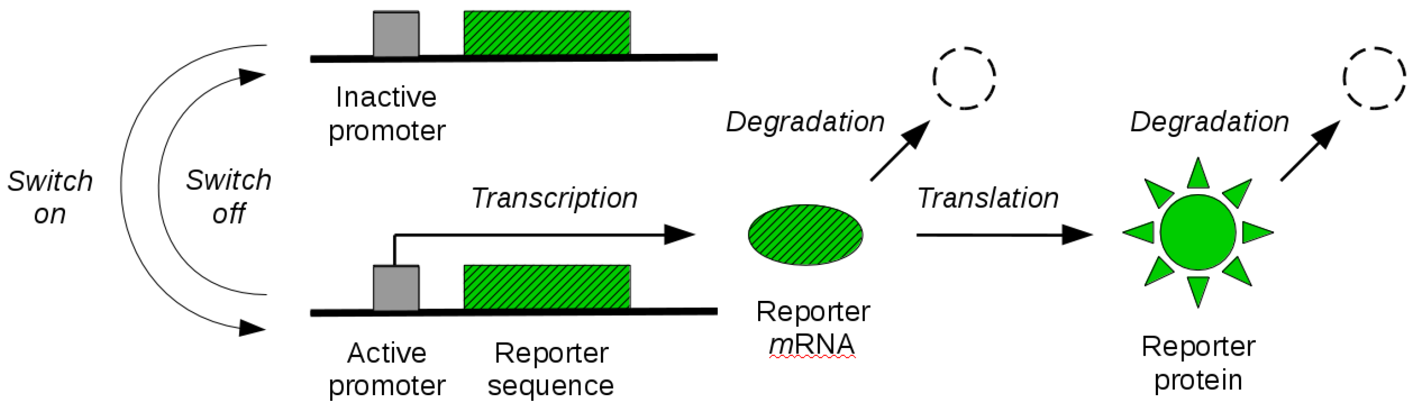
By the tools developed in the previous sections, in this section, we study identifiability of reporter gene systems. These are synthetic gene constructs that are commonly engineered into cells to monitor gene expression over time in terms of the synthesis of a fluorescent (or luminescent) protein [36]. The illustration of a reporter gene is given in Figure 1. When the gene is expressed, the transcription of the genetic sequence that codes for the fluorescent protein leads to synthesis of corresponding mRNA molecules. These molecules are then transcribed in a second step, leading to the synthesis of fluorescent proteins. When the gene is switched off, synthesis of mRNA molecules is no longer possible until the gene is switched on again. The existing mRNA and protein molecules are subject to degradation throughout. Experimental measurement of fluorescence intensity allows for the quantification of the abundance of fluorescent reporter molecules over time, and thus gives an indirect dynamical readout of the gene expression state. In some cases, an additional maturation step of the reporter protein needs to be taken into account before the molecule becomes fluorescent. While this can be modelled in our mathematical framework, we will not address it here.

Let M and P denote mRNA and protein species, in the same order. Let F be the active promoter species, such that gene expression is enabled only when F is present. The synthesis and degradation of mRNA and protein molecules described above are typically expressed by the reaction model

$$\begin{array}{cccc}\hfill F& \stackrel{k_M}{\to }F+M,\hfill & \hfill M& \stackrel{d_M}{\to }⌀,\hfill \end{array}$$

(19)

$$\begin{array}{cccc}\hfill M& \stackrel{k_P}{\to }M+P,\hfill & \hfill P& \stackrel{d_P}{\to }⌀,\hfill \end{array}$$

(20)

for some nonnegative rate parameters $k_M$, $k_P$, $d_M$ and $d_P$ [14,37]. In turn, for some nonnegative parameters ${\lambda }_{+}$ and ${\lambda }_{-}$, the switching dynamics of F are expressed by two additional reactions for activation and deactivation,

$$\begin{array}{cccc}\hfill ⌀& \stackrel{r\left({\lambda }_{+}\right)}{\to }F,\hfill & \hfill F& \stackrel{{\lambda }_{-}}{\to }⌀,\hfill \end{array}$$

(21)

where the activation rate parameter $r\left({\lambda }_{+}\right)$ is equal to ${\lambda }_{+}$ in the inactive state, and to 0 otherwise (activation is possible only from the inactive state).

At the level of single cells, Equations (19)–(21) are known as the random telegraph model of gene expression [14]. Let $X_1\in \mathbb{N}$ and $X_2\in \mathbb{N}$ be the number of molecules of species M and P, respectively. Let $X_3\in \{0,1\}$ be the state of the gene promoter, that is, $X_3=0$ in the inactive state and $X_3=1$ in the active state. In accordance with the modelling of Section 2, one may describe $X={\left[X_1{X}_2{X}_3\right]}^T$ as a Markov process [14]. The rates of the $m=6$ reactions (19)–(21) (ordered from left to right, top to bottom) are

$$a(x,t)={\left[\begin{array}{cccccc}{k}_M{x}_3& d_M{x}_1& k_P{x}_1& d_P{x}_2& {\lambda }_{+}(1-x_3)& {\lambda }_{-}{x}_3\end{array}\right]}^T.$$

These rates are in the affine form (1), with time-independent $w_0\left(t\right)=G$. Rate parameters and stoichiometry matrix of the network are

$$\begin{array}{ccccc}\hfill S& =\left[\begin{array}{cccccc}1& -1& 0& 0& 0& 0\\ 0& 0& 1& -1& 0& 0\\ 0& 0& 0& 0& 1& -1\end{array}\right],\hfill & \hfill W& =\left[\begin{array}{ccc}0& 0& k_M\\ d_M& 0& 0\\ k_P& 0& 0\\ 0& d_P& 0\\ 0& 0& -{\lambda }_{+}\\ 0& 0& {\lambda }_{-}\end{array}\right],\hfill & \hfill G=\left[\begin{array}{c}0\\ 0\\ 0\\ 0\\ {\lambda }_{+}\\ 0\end{array}\right].\end{array}$$

We consider that all rate parameters of reactions (19)–(21), that is all parameters defining W and G, are unknown, and wish to study their identifiability from the experimentally observed species P. The observation model (7), that is, matrix C, is thus such that $y\left(t\right)={\left[\mathbb{E}\left[X_2\left(t\right)\right],\mathrm{var}\left(X_2\left(t\right)\right)\right]}^T$. We first investigate structural identifiability by the approach of Section 3.1. This requires in the first place to compute the Laplace transform $Y(s,\theta )$ and its sensitivity function $\nabla Y(s,\theta )$. We implemented these computations in Matlab (Release 2017b, The MathWorks, Inc., Natick, MA, USA) by the aid of the Symbolic calculation toolbox. Because $Y(s,\theta )$ is a rational (vector) function, this allows us to obtain explicit expressions for $\nabla Y(s,\theta )$ in the symbolic variables s and $\theta$ in a straightforward manner. Then, for a given set of test points ${\mathcal{S}}_L$ and a given vector ${\theta }^{\ast }$, we evaluate $\nabla Y(s,\theta )$ numerically at $(s,\theta )=(s_{\ell },{\theta }^{\ast })$, for all values $s_{\ell }\in {\mathcal{S}}_L$. This allows us to build the sensitivity matrix $\Delta ({\mathcal{S}}_L,{\theta }^{\ast })$ and finally compute its rank. In the light of Corollary 1, the system is found identifiable if this rank is full.

For our case study, given the number of test points L, matrix $\Delta ({\mathcal{S}}_L,\theta )$ has $2L$ rows. Therefore, the full column rank required by Corollary 1 to conclude for identifiability can only be obtained if $2L\ge N$, where N, the number of columns of $\Delta ({\mathcal{S}}_L,\theta )$, is equal to the size of the parameter vector $\theta$. This is made of six rate parameters plus the unknown initial conditions $z_0$, for a total of $N=15$ entries. Then, identifiability should be tested with $L\ge 8$. We arbitrarily set $L=10$ and choose points ${\mathcal{S}}_L=\{s_l=l:l=1,\dots ,L\}$. Then, we sampled values ${\theta }^{\ast }$ at random and computed the corresponding rank of $\Delta ({\mathcal{S}}_L,{\theta }^{\ast })$. We always found this rank to be full, that is, we concluded in each case that the reporter gene system is structurally locally identifiable. Whereas one such random evaluation suffices, the consistency of the result shows the effectiveness of the method, which does not depend on a critical choice of ${\theta }^{\ast }$ or ${\mathcal{S}}_L$.

To verify how variance observations contribute to identifiability, by the same approach, we further investigated structural local identifiability from the observation of the reporter abundance (fluorescence) mean only. The method holds unchanged, provided a suitable redefinition of matrix C. In this case, $\Delta ({\mathcal{S}}_L,\theta )$ has only L rows, and its rank should be tested for $L\ge N$. For increasing values of L and parameter values ${\theta }^{\ast }$ sampled at random as above, the maximal rank of this reduced version of $\Delta ({\mathcal{S}}_L,{\theta }^{\ast })$ was found to be equal to 7. That is, full column rank was never found. Since the rank condition of Corollary 1 is not necessary but only sufficient, we cannot state from this test that the reporter system lacks structural identifiability from the mean, yet the results are a strong hint toward non-identifiability. In fact, consider for simplicity $z_0=0$. The entry of $Y(s,\theta )$ associated with the mean is found to be

$${\lambda }_{+}{k}_M{k}_P/\left[s({\lambda }_{+}+{\lambda }_{-}+s)(d_M+s)(d_P+s)\right].$$

Inspection of this formula reveals lack of identifiability, since parameters $k_M$ and $k_P$ only appear through the product $k_M{k}_P$. Thus, in this case, it is easy to see that changes in one parameter can be perfectly compensated by reciprocal changes in another parameter, such that unique values for these parameters cannot be fixed from the available observations.

To summarize, by the identifiability test of Section 3.1, we showed that the observation of reporter protein mean and variance profiles guarantees structural identifiability of the gene expression model, whereas the same model is not structurally identifiable from the mean only. This is similar to an analogous result in [8], where, however, global structural identifiability of a simpler gene expression model not accounting for switching promoter dynamics is investigated. Note that, for our case study, assessing global identifiability is rather challenging. For instance, by the existing approaches based on (13) [1,31], one would be confronted with an algebraic analysis of $Y(s,\theta )$, whose second entry is a ratio of polynomials of degree 10. Our local identifiability result was instead obtained by a symbolic computation approach that is fast, robust and fully general, as it can equally deal with any network in the class we consider.

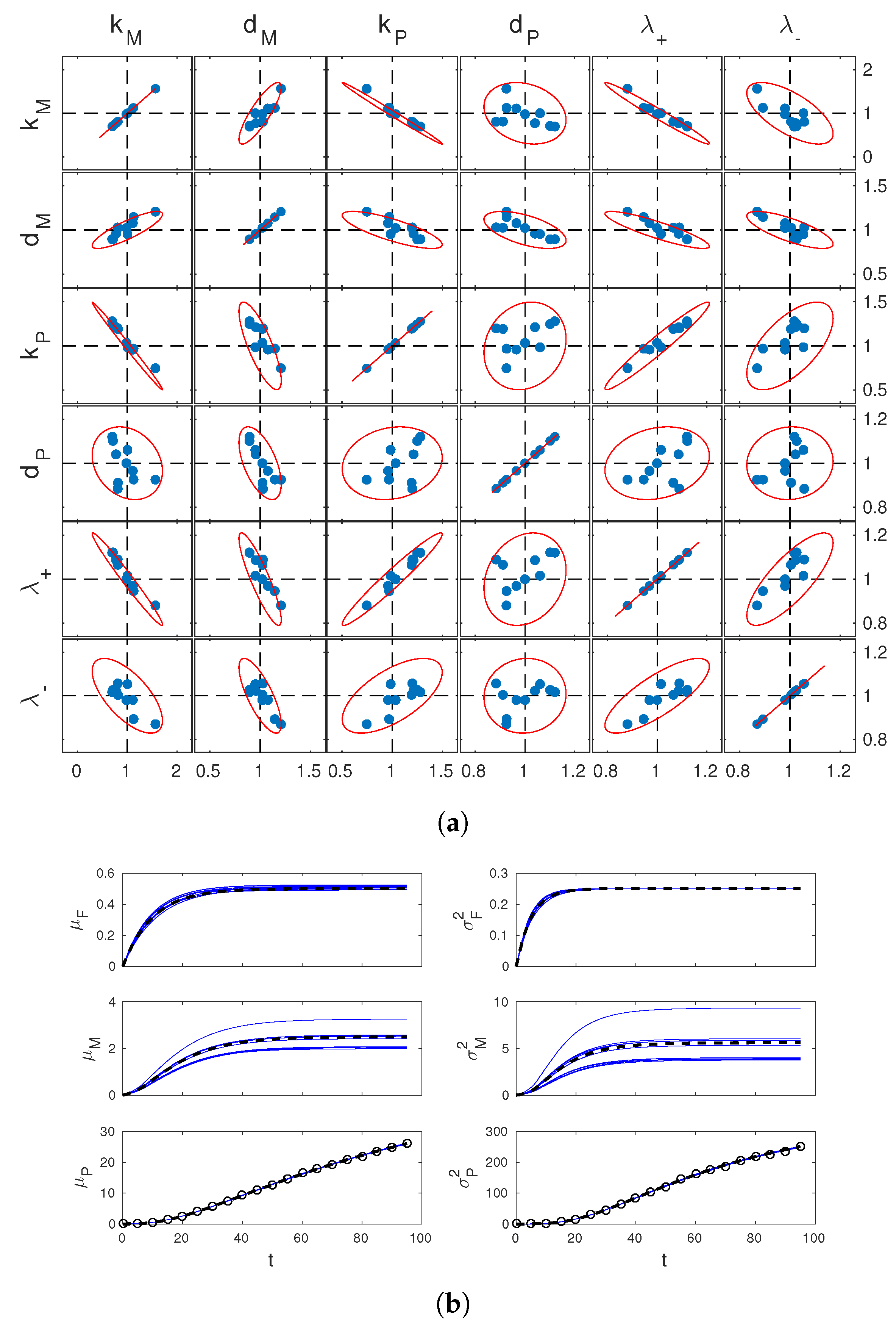
For the same system, we now move on to a practical analysis of identifiability by the tools reported in Section 3.2. For simplicity, we fixed $z_0=0$ and assumed it known. We set the value of the rate parameters to ${\theta }^{\ast }=(k_M,d_M,k_P,d_P,{\lambda }_{+},{\lambda }_{-})=(0.5,0.1,0.2,0.01,0.05,0.05)$ (in minutes${}^{-1}$). These values are consistent with the literature [36,37] and correspond to a case of slow switching of the gene expression state and a stable reporter protein. (At this ${\theta }^{\ast }$, the system is locally identifiable.) For convenience, let us denote by ${\mu }_P$ and ${\sigma }_P^2$ respectively the mean and variance of $X_2$ (the abundance of the reporter protein P), and use similar notation for the other species F and M. Simulated data were generated for this system for $t\in [0,95]$ (minutes). Random simulations were performed in StochKit [38]. We fixed measurement times to $t_{\ell }=(\ell -1)·5$ min, with $\ell =1,\dots ,N_y$ and $N_y=20$. At these times, we computed empirical mean and variance statistics of $X\left(t\right)$ from ${10}^4$ simulated trajectories (different simulations were used at different measurement times to mimic statistically independent cell samples across ℓ). This allowed us to to generate measurements of ${\mu }_P$ and ${\sigma }_P^2$ of the type (8) and (9). The obtained data is exemplified in Figure 2b. Based on 10 such datasets, we estimated ${\theta }^{\ast }$ 10 times by numerical solution of (16). Estimation was performed in Matlab (fmincon, with initial guess $5·{\theta }^{\ast }$). Results are reported in Figure 2a together with $95\%$ confidence regions determined from (18).

First of all, it can be seen that the confidence regions deduced from the approximate estimation error covariance matrix V are in excellent agreement wth simulated estimates. Therefore, they provide an effective tool to study practical identifiability. In our case, one sees from the figure that the confidence regions for the joint estimation of $k_M$ and $k_P$ are nearly degenerate ellipses. Relating this with the structural identifiability analysis carried out before, one concludes that, whereas variance observations guarantee identifiability of the system, discerning $k_M$ and $k_P$ unambiguously from their product $k_M{k}_P$ remains difficult. Further analysis of Figure 2a shows that discerning ${\lambda }_{+}$ from $k_M$ and $k_P$ is also difficult. This is not surprising since ${\lambda }_{+}$ itself multiplies $k_M$ and $k_P$ in the entry of $Y(s,\theta )$ displayed above (however ${\lambda }_{+}$ also appears at the denominator separate from the other parameters). Finally, it is interesting to look at the time profiles of the statistics of M and F corresponding to the 10 estimates of ${\theta }^{\ast }$. These are shown in Figure 2b. The estimates of ${\mu }_F(·)$ and ${\sigma }_F^2(·)$ are all close to the true profiles, while those of ${\mu }_M(·)$ and ${\sigma }_M^2(·)$ are significantly more dispersed. Apparently, the limited accuracy in the estimation of $k_M$, $k_P$ and ${\lambda }_{+}$ is reflected in the estimates of the mRNA statistics, but not in those of gene activation statistics. This shows that, depending on the purpose of parameter identification, inaccurate parameter estimates may or not be detrimental for the study of the system.

In summary, the study of practical identifiability of the reporter gene system showed that structural identifiability translates into the ability to discern all parameters unambiguously, but with an accuracy that still depends on the interplay of the parameters. Moreover, certain system dynamics may still be predicted with accuracy in spite of poor estimates of relevant system parameters. This relates with the concept of “parameter sloppiness” discussed in the literature for biological systems [5].

4. Identification of Networks

As discussed in Section 2, the structure of regulatory interactions among species of a given network is captured by the pattern of nonzero entries of S and W. In Section 3, we have discussed the problem of identifying unknown parameters of a reaction network with a known structure of interactions. By the case study of Section 3.3, we have shown that usage of stochastic information, such as the dynamics of the network state variance, may guarantee structural parameter identifiability in cases where the sole usage of deterministic information, such as the mean system response, does not. In this section, we wish to investigate whether the addition of stochastic information also helps identification of networks with unknown interactions. In full generality, the problem thus becomes the identification of the matrices $S\in {\mathbb{Z}}^{n\times m}$ and $W\in {\mathbb{R}}^{m\times n}$, defining models (10) and (11) via (5), from measurements of type (8). Matrix C, describing what statistical moments are observed for what species, is fixed by the measurement experiment design and is thus known.

In a first, naive attempt, one could approach identification of S and W by directly fitting measurements (8) with the predictions of (10) and (11). However, this is computationally intensive, since it requires solving the dynamics (10) repeatedly over the joint search space of S and W, and does not give any insight into the identifiability of S and W. On the other hand, Equations (10) and (11) are a linear dynamical system. Disregarding the specific structure of A and B, linear dynamical systems can be reconstructed by standard identification techniques [31,39]. This suggests separating identification of S and W into two steps. The first step is the reconstruction of a dynamical model in the form

$$\begin{array}{cc}\hfill \dot{\xi }\left(t\right)& =\widehat{A}\xi \left(t\right)+\widehat{K}u\left(t\right),\hfill \\ \hfill y\left(t\right)& =\widehat{C}\xi \left(t\right),\hfill \end{array}$$

(22)

from measurements (8). For noiseless measurements, one such model perfectly matching the data is of course given by Equations (10) and (11), with $z=\xi$, $\widehat{A}=A$, $\widehat{K}=BG$ and $\widehat{C}=C$. Assuming for a moment that the reconstructed $\widehat{A}$ equals A and $\widehat{K}=BG$, the second step is the inference of S and W from $\widehat{A}$ and $\widehat{K}$ in light of Equation (5). A similar approach is used for parameter estimation of a known network in [30].

A priori, none of the two steps has a unique solution. In the first step, several models $(\widehat{A},\widehat{K},\widehat{C})$ may equally explain the same data, that is, $\widehat{A}$ and $\widehat{K}$ may not be uniquely defined (even their dimension is generally not uniquely determined). In addition, noise on measurement samples propagates into the computation of $\widehat{A}$, $\widehat{K}$. In the second step, leaving G aside for the moment, the crucial question is whether the matrices S and W that define the network structure can be uniquely factored out of $\widehat{A}$. As we will see, the answer depends in the first place on the relationship between $\widehat{A}$ and A.

In analogy with the discussion of Section 3.1, we will first look at the problem in terms of identifiability from $y(·)$ and $u(·)$. In Section 4.1, we will look at the reconstruction problem of a suitable model in the form (22). In Section 4.2, we will look at the subsequent problem of extracting S and W from the reconstructed $\widehat{A}$. In order to understand how stochasticity contributes to the reconstruction of unknown networks, in these two sections, we will focus on a first case, where $y(·)=\mu (·)$, and a second case, where observations additionally include the entries of $\Sigma (·)$, that is, $y(·)=z(·)$. Then, in Section 4.3, we will look at these two steps from a practical perspective, providing a method to infer S and W from real data. The contribution of stochasticity to the identifiability of S and W and the full network identification procedure will be demonstrated on an example in Section 4.4. We will assume throughout this section that $u\left(t\right)$ is assigned, leaving experiment design considerations to later studies (see Section 5).

4.1. Step 1: Identifiability of a Linear Model for the Moment Dynamics

Here, we are concerned with the reconstruction of a model in the form (22). Let us recall some facts [40]. In the context of linear state-space models, a realization of a (strictly causal) linear map $\mathcal{L}:\mathcal{U}\to \mathcal{Y}$ from an input space $\mathcal{U}$ to an output space $\mathcal{Y}$ is any triplet $(\widehat{A},\widehat{K},\widehat{C})$ such that the solution of (22) reproduces this mapping. Its order is the size of matrix $\widehat{A}$. It is well known that, if $(\widehat{A},\widehat{K},\widehat{C})$ is one realization, all triplets $(T\widehat{A}{T}^{-1},T\widehat{K},\widehat{C}{T}^{-1})$, with T a nonsingular square matrix, are equally viable realizations. A realization is minimal if it has the smallest size of $\widehat{A}$ among all realizations. If $(\widehat{A},\widehat{K},\widehat{C})$ is minimal, then all minimal realizations are of the form $(T\widehat{A}{T}^{-1},T\widehat{K},\widehat{C}{T}^{-1})$ for some nonsingular T, i.e., minimal realizations form an equivalence class.

Recall that $n_y$ is the number of rows of C, that is, the size of vector y. We will make the following assumption.

Assumption 1.

The minimal realization of the linear map expressed by (10) and (11) is of order greater than or equal to$n_y$. In addition, for the given u, the class of minimal realizations is uniquely determined by u and the corresponding y.

The first part of this assumption concerns structural properties of the system, essentially ruling out singular cases where the moment equations provide a redundant description of the dynamics of y. As a counterexample, a system that would not fulfill this requirement is one where two observed species participate in the same reaction in exactly the same way, such that the evolution of their moments is identical. On the basis of the first part, the second part of the assumption concerns the informativity of the given input–output pair, requiring in practice that all observed moments are excited by the given input. In view of the relation between minimal realizations and transfer functions, this corresponds to saying that the system transfer function can be identified from the given input–output pair. This is a reasonable requirement provided a sufficiently rich excitation input [39,40].

In summary, under Assumption 1, identification is well-posed up to an unknown matrix T. However, if $(\widehat{A},\widehat{K},\widehat{C})$ is a minimal realization determined from u and y, T is constrained by the knowledge of C, since it must hold that $\widehat{C}{T}^{-1}=C$. What this constraint implies on the reconstructed model depends on how a minimal realization of the system itself looks like. We focus on the following cases:

Case (i):

Observation of mean only ($y=\mu$). In this case, $n_y=n$ and $C=\left[\begin{array}{cc}{C}^{\prime }& 0_{n\times n^2}\end{array}\right]$, with $C^{\prime }\in {\mathbb{R}}^{n\times n}$ nonsingular (typically the identity). In view of the structure of A in (5), for this definition of C, one realization of (10) and (11) is

$$\begin{array}{cc}\hfill \dot{\xi }\left(t\right)& =SW\xi \left(t\right)+SGu\left(t\right),\hfill \\ \hfill y\left(t\right)& =C^{\prime }\mu \left(t\right).\hfill \end{array}$$

This realization is of order $n_y=n$ and is minimal for non-degenerate definitions of S, W and G. Assumption 1 is thus satisfied provided the input and/or the initial conditions excite all system dynamics. Then, any reconstructed model $(\widehat{A},\widehat{K},\widehat{C})$ must satisfy $(\widehat{A},\widehat{K},\widehat{C})=(TSW{T}^{-1},TSG,C^{\prime }{T}^{-1})$ for some invertible T. Since $C^{\prime }$ is known and invertible, $T={\widehat{C}}^{-1}{C}^{\prime }$ is uniquely determined, and so are $SW=T^{-1}\widehat{A}T$ and $SG=T^{-1}\widehat{K}$.

Case (ii):

Observation of mean and covariance matrix ($y=z$). Since $\Sigma ={\Sigma }^T$, this case is captured by a model where C has $n_y=n+n(n+1)/2$ rows and $n+n^2$ columns. The definition of C is such that $y=Cz=C^{″}\xi$, where $\xi$ is an $n_y$-dimensional vector containing all and only the distinct entries of z, and $C^{″}$ is invertible (in particular, C and $C^{″}$ can be $(0,1)$-matrices). One realization of (10) and (11) is then

$$\begin{array}{cc}\hfill \dot{\xi }\left(t\right)& =A^{″}\xi \left(t\right)+K^{″}u\left(t\right),\hfill \\ \hfill y\left(t\right)& =C^{″}{\xi }^{″}\left(t\right),\hfill \end{array}$$

where $A^{″}$ and $K^{″}$ are formed from all and only the distinct entries of A and $BG$, in the same order, in accordance with the definition of $\xi$. This realization is of order $n_y$, and is minimal except for peculiar definitions of S and W. Similar to Case (i), provided Assumption 1 is satisfied, any reconstructed model $(\widehat{A},\widehat{K},\widehat{C})$ must satisfy $(\widehat{A},\widehat{K},\widehat{C})=(T{A}^{″}{T}^{-1},T{K}^{″},C^{″}{T}^{-1})$, with T invertible. Because $C^{″}$ is known, by the same arguments used in Case (i), matrices $A^{″}$ and $K^{″}$ are uniquely determined. Since they necessarily contain all elements of A and $BG$, the latter are also uniquely determined.

In summary, under Assumption 1, Case (i) guarantees unambiguous reconstruction of the products $SW$ and $SG$, while Case (ii) also guarantees unambiguous reconstruction of the other blocks of A, namely $S^{\left(2\right)}W$ and $I_n\otimes \left(SW\right)+\left(SW\right)\otimes I_n$, and of the second block of $BG$, namely $S^{\left(2\right)}G$. Other cases of interest exist, among which, for instance, the observation of the statistics of part of X, or the observation of the diagonal entries of $\Sigma$ only [8,9,18]. The investigation of these scenarios is beyond the scope of this paper, but is rediscussed in Section 5.

4.2. Step 2: Identifiability of the Network Stoichiometry and Rate Parameter Matrices

We have shown in the previous section that different information about the matrices of model (10) and (11) can be obtained depending on the definition of matrix C. This can be summarized in terms of the $(n+n^2)\times (n+n_u)$ matrix

$$\Xi (S,W,G)\triangleq \left[\begin{array}{cc}SW& SG\\ S^{\left(2\right)}W& S^{\left(2\right)}G\end{array}\right].$$

(23)

Under Assumption 1, Case (i) yields perfect reconstruction of the first block-row (first n rows) of $\Xi (S,W,G)$, whereas Case (ii) also yields the remaining $n^2$ rows. Note that, for the latter case, the further availability of $I_n\otimes \left(SW\right)+\left(SW\right)\otimes I_n$ does not provide additional information since the product $SW$ is already part of the first n rows of $\Xi (S,W,G)$. For these two cases, the question addressed in this section is what can be said about the individual contributions of S, W and G.

Denote with ${\Xi }_h(S,W,G)$ the first h rows of (23). For $h=n$ and $h=n+n^2$, in the order, denote with ${\widehat{\Xi }}_h$ the estimate of ${\Xi }_h(S,W,G)$ obtained in Step 1 for Case (i) and Case (ii), in the same order. Under the current hypothesis of perfect reconstruction, it holds that

$${\widehat{\Xi }}_h={\Xi }_h(S,W,G).$$

(24)

The question we are posing is about the solutions $(S,W,G)$ of $\left(\right)$ given ${\widehat{\Xi }}_h$. One solution to (24) is of course provided by the true network matrices, which we denote $S^{\ast }$, $W^{\ast }$, $G^{\ast }$. Equivalent solutions are all triplets $(S,W,G)$ obtained by permutation of the columns of $S^{\ast }$ and corresponding permutation of the rows of $W^{\ast }$ and $G^{\ast }$, since these are trivially different enumerations of the network reactions ${\mathcal{R}}_1,\dots ,{\mathcal{R}}_m$. However, other solutions may exist. Simple algebraic manipulations of (23) and (24) yield

$$\begin{array}{cccc}\hfill {\widehat{\Xi }}_h& =L_h\left(S\right)·\left[\begin{array}{cc}W& G\end{array}\right],\hfill & \hfill L_h\left(S\right)& \triangleq \mathrm{first}h\mathrm{rows}\mathrm{of}\left[\begin{array}{c}S\\ S^{\left(2\right)}\end{array}\right].\hfill \end{array}$$

(25)

Thus, for a given ${\widehat{\Xi }}_h$, the viable triplets $(S,W,G)$ are all solutions to the mixed factorization problem (25) with discrete-valued factor $L_h\left(S\right)$ and continuous-valued factor $\left[WG\right]$. Clearly, the set of solutions is generally smaller the larger the h, since more equations need to be satisfied. That is, Case (ii) has better potential than Case (i) for precise network reconstruction. Starting from (25), a characterization of the solutions in terms of algebraic or topological properties of the true underlying network would be desirable but is still unavailable to us. Our contribution here is an operational definition of all possible solutions, that is, an algorithmic procedure to seek all solutions corresponding to a given ${\widehat{\Xi }}_h$.

Let $\mathbb{S}\subseteq {\mathbb{Z}}^{n\times m}$, $\mathbb{W}\subseteq {\mathbb{R}}^{m\times n}$ and $\mathbb{G}\subseteq {\mathbb{R}}^{m\times n_u}$, with $\mathbb{W}$ and $\mathbb{G}$ convex. For any matrix norm $\left|\right||·|\left|\right|$, if $S^{\ast }\in \mathbb{S}$, $W^{\ast }\in \mathbb{W}$ and $G^{\ast }\in \mathbb{G}$, the solutions of (25) coincide with the set of optimizers of

$$\begin{array}{cccc}\hfill Q^{\ast }& \triangleq \underset{(S,W,G)\in \mathbb{S}\times \mathbb{W}\times \mathbb{G}}{min}Q(S,W,G),\hfill & \hfill Q(S,W,G)& \triangleq \left|\right||{\widehat{\Xi }}_h-L_h\left(S\right)·\left[WG\right]\left|\right||,\hfill \end{array}$$

(26)

and $(S^{\ast },W^{\ast },G^{\ast })$ attains the minimum $Q^{\ast }=0$. Problem (26) can be rewritten as

$$\begin{array}{cc}\hfill Q^{\ast }& =\underset{S\in \mathbb{S}}{min}\widehat{Q}\left(S\right),\hfill \end{array}$$

(27)

$$\begin{array}{cc}\hfill \widehat{Q}\left(S\right)& \triangleq \underset{(W,G)\in \mathbb{W}\times \mathbb{G}}{min}Q(S,W,G).\hfill \end{array}$$

(28)

For any fixed S, Equation (28) is a least-squares problem with convex constraints that is easy to solve by standard search algorithms [41]. For finite $\mathbb{S}$, the complete solution space of (27) can then be determined by exploration of $\mathbb{S}$, seeking all S such that $\widehat{Q}\left(S\right)=0$. In general, the solution of (28) is not unique. If S is such that $\widehat{Q}\left(S\right)=0$ and $(W,G)$ solves the corresponding problem (28), then all couples $(W+\tilde{W},G+\tilde{G})\in \mathbb{W}\times \mathbb{G}$ such that the columns of $[\tilde{W}\tilde{G}]$ are in $ker\left(L_h\left(S\right)\right)$ (“$ker(·)$” denotes the kernel of a matrix) equally solve (28). The multiplicity of the solutions for a given S thus depends on the interplay between $ker\left(L_h\left(S\right)\right)$ and $\mathbb{W}\times \mathbb{G}$. We will come back on this in the example of Section 4.4.

For all practical matters (robustness to numerical errors and modelling inaccuracies, and applications below where ${\widehat{\Xi }}_h$ is computed from the noisy data (8), one should require that the equality in (25) holds approximately within a suitable tolerance $ϵ>0$. This leads to the procedure for the computation of the set of solutions $\Omega$ detailed in Algorithm 1.

One possible choice of $\mathbb{S}$ is to consider all matrices $S\in {\mathbb{Z}}^{n\times m}$ whose elements $S_{i,j}$ are such that, for some $S_{max}\in \mathbb{N}$, $|S_{i,j}|\le S_{max}$, with $i=1,\dots ,n$ and $j=1,\dots ,m$. The size of $\mathbb{S}$ in this case is of order $\mathcal{O}\left(S_{max}^{nm}\right)$. Despite the exponentially growing complexity, exploring $\mathbb{S}$ by enumeration remains viable for networks of small size. The complexity of this search could be dramatically reduced by recalling that permutations of the reactions list amount to equivalent models. Other ameliorations are possible to improve the scalability of the method (see also the relevant discussion in Section 5).

Algorithm 1: Identification of stoichiometry and rate parameters from a model of the moment dynamics

Given ${\widehat{\Xi }}_h$ and an $ϵ>0$:

Set $\Omega =\varnothing$;

For every $S\in \mathbb{S}$:

Solve problem (28) to get $\widehat{Q}\left(S\right)$ and the solution set $\widehat{\Omega }\left(S\right)=\{(W,G):Q(S,W,G)=\widehat{Q}\left(S\right)\}$;

If $\widehat{Q}\left(S\right)<ϵ$, include $\left\{S\right\}\times \widehat{\Omega }\left(S\right)$ in $\Omega$;

Return $\Omega$.

To conclude, suppose that the true number of reactions, say $m^{\ast }$, is unknown. One way to generalize the procedure above to this scenario is to execute it for a value of m large enough. By this approach, let $\widehat{m}\le m$ be the minimum number of nonzero columns of S among the elements of $\Omega$. Since the null columns of S do not contribute to the network dynamics, $\widehat{m}$ is the minimum number of reactions needed to explain the data and is thus a viable estimate of m. In practice, though, this approach is computationally inefficient, since it explores an unnecessarily large space $\mathbb{S}$. A better solution is to proceed incrementally and execute the algorithm for increasing values of m, stopping the exploration as soon as $\Omega \ne \varnothing$.

4.3. Network Identification in Practice

So far in this section, we have treated reconstruction of moment dynamics (Step 1) and then of biochemical network matrices (Step 2) in the absence of noise. We now devise a procedure for the two-step estimation of S, W and G from noisy moment measurements of the types (8) and (9). To do this, we will repeatedly exploit the methods of Section 3.2, with a specific definition of parameters $\theta$. For ease of exposition, we focus on Case (ii) and assume that the initial system moments $z_0$ are known. The generalization to possible unknown entries of $z_0$ is straightforward. The necessary adaptations for Case (i) are commented on at the end of the section.

Consider Step 1 first. As mentioned in Section 4.1, general approaches to the estimation of linear state-space models can be borrowed from literature. Here, however, we account explicitly for the structure of model (5) and develop a dedicated approach. Let ${\theta }_{1,1}$, ${\theta }_{1,2}$, ${\theta }_{2,1}$ and ${\theta }_{2,2}$ denote the unknown matrix products $SW$, $SG$, $S^{\left(2\right)}W$ and $S^{\left(2\right)}G$ that compose (23), in the same order, and let $\theta$ be the vector collecting all entries of ${\theta }_{1,1}$, ${\theta }_{1,2}$, ${\theta }_{2,1}$ and ${\theta }_{2,2}$. Define ${\widehat{y}}_{\theta }(·)$ as the solution of

$$\begin{array}{cccc}\hfill \frac{d}{dt}{\widehat{z}}_{\theta }& =\left[\begin{array}{cc}{\theta }_{1,1}& 0\\ {\theta }_{2,1}& I_n\otimes {\theta }_{1,1}+{\theta }_{1,1}\otimes I_n\end{array}\right]{\widehat{z}}_{\theta }+\left[\begin{array}{c}{\theta }_{1,2}\\ {\theta }_{2,2}\end{array}\right]u\left(t\right),\hfill & \hfill {\widehat{z}}_{\theta }\left(0\right)& =z_0,\hfill \end{array}$$

(29)

$$\begin{array}{cc}\hfill {\widehat{y}}_{\theta }& =C{\widehat{z}}_{\theta }.\hfill \end{array}$$

(30)

Note that, for true parameter values, these equations coincide with the true moment dynamics (10) and (11). With these definitions of $\theta$ and ${\widehat{y}}_{\theta }$, for a suitable search space $\Theta$, we compute the ML estimate $\widehat{\theta }$ by the solution of (16), which provides us with estimates of $SW$, $SG$, $S^{\left(2\right)}W$ and $S^{\left(2\right)}G$. In practice, this solution shall be computed by numerical optimization.

Now, consider Step 2. The estimates $\widehat{\theta }$ of $SW$, $SG$, $S^{\left(2\right)}W$ and $S^{\left(2\right)}G$ from above allow us to build (a noisy version of) the matrix ${\widehat{\Xi }}_h$ of Section 4.2 (with $h=n+n^2$ for Case (ii)). This matrix can be used to run Algorithm 1 and determine a set of solution triplets $(S,W,G)$. However, for a candidate solution $(S,W,G)$, the acceptance criterion $Q(S,W,G)<ϵ$ (with $Q(S,W,G)=\left|\right||{\widehat{\Xi }}_h-L_h\left(S\right)·[W,G]\left|\right||$) needs to be adapted to the statistics of the noise that corrupts ${\widehat{\Xi }}_h$. To do this, we first compute the estimation error covariance matrix for ${\widehat{\Xi }}_h$, say $V_h$, by the sensitivity method explained after (16). Armed with $V_h$, for a given confidence level $1-\alpha$, the idea is to define the norm $\left|\right||·|\left|\right|$ and $ϵ$ such that a candidate solution $(S,W,G)$ is accepted by Algorithm 1 if the discrepancy between $L_h\left(S\right)·\left[WG\right]$ and ${\widehat{\Xi }}_h$ falls within the $(1-\alpha )$-confidence ellipsoid around ${\widehat{\Xi }}_h$. In view of (18), this is obtained by setting $ϵ={\chi }_{\alpha }$ and

$$Q(S,W,G)=\mathrm{vec}{\left({\widehat{\Xi }}_h-L_h\left(S\right)·\left[WG\right]\right)}^T{V}_h^{-1}\mathrm{vec}\left({\widehat{\Xi }}_h-L_h\left(S\right)·\left[WG\right]\right).$$

In this way, our acceptance criterion is expressed as a ${\chi }^2$-statistical test that the candidate solution corresponds to the true parameters underlying our estimate ${\widehat{\Xi }}_h$.

For Case (i), the method described above remains the same, except that $\theta$ shall only contain the entries of ${\theta }_{1,1}$ and ${\theta }_{1,2}$, model (29) and (30) is restricted to the mean dynamics, and ${\widehat{\Xi }}_h$, $L_h$ are defined for $h=n$. From a computational viewpoint, our two-step approach requires fitting moment equations to measurements (8) only once (Step 1). On the contrary, the naive approach discussed at the beginning of Section 4 would require solving a similar optimization problem iteratively for all the candidate stoichiometries S. Our approach postpones this search to the second step based on the iterative solution of a much simpler, convex optimization problem, with tremendous computational saving. Observe that the error statistics in the estimation of matrix products $S^{\ast }{W}^{\ast }$ and ${\left(S^{\ast }\right)}^{\left(2\right)}{W}^{\ast }$ from Step 1 are quantitatively accounted for in the construction of the test to select the compatible network structures in Step 2. Therefore, provided the ML estimator in Step 1 is close to optimality, the splitting of network identification into two steps is not expected to deteriorate performance relative to a one-step procedure testing candidate network structures directly on the moment measurements.

In summary, we have devised an algorithm to perform reconstruction of biochemical networks from real-world population-snapshot data. The method can be applied to mean data only, but, contrary to existing approaches, it equally applies to joint mean and variance measurements. We argued by theoretical arguments that leveraging the additional variance measurements is expected to improve reconstruction accuracy. In the next section, we will show that this is indeed the case by the analysis of a case study, which reconfirms the practical interest of our method.

4.4. Example: A Toy Network

We now apply the methods developed above to a toy example. Our first aim is to study the achievable network reconstruction performance in Case (i) (observations of mean only) and (ii) (observations of mean and covariance matrix). To do this, we initially focus on the network reconstruction step described in Section 4.2, assuming that the matrix products $S^{\ast }{W}^{\ast }$ and, for Case (ii), ${\left(S^{\ast }\right)}^{\left(2\right)}{W}^{\ast }$ are known exactly. For simplicity, we ignore G. This constitutes no loss of generality since G enters the factorization problem (25) in a way similar to W. Our second aim is to test the full identification procedure of Section 4.3, where the products $S^{\ast }{W}^{\ast }$ and ${\left(S^{\ast }\right)}^{\left(2\right)}{W}^{\ast }$ are not known and need to be estimated from noisy measurements of the network moments. This is done at the end of the section on the basis of simulated data.

Consider a reaction network with

$$S^{\ast }=\left[\begin{array}{ccc}-1& 0& 0\\ 1& 1& -1\end{array}\right],W^{\ast }=\left[\begin{array}{cc}0.2& 0\\ 0.1& 0\\ 0& 0.1\end{array}\right],$$

where superscript “${}^{\ast }$” denotes true system quantities. The actual network size is then $n^{\ast }=2$ and $m^{\ast }=3$. For this system, the matrix products defining the moment dynamics are

$$\begin{array}{cccc}\hfill S^{\ast }{W}^{\ast }& =\left[\begin{array}{cc}-0.2& 0\\ 0.3& -0.1\end{array}\right],\hfill & \hfill {\left(S^{\ast }\right)}^{\left(2\right)}{W}^{\ast }& =\left[\begin{array}{cc}0.2& 0\\ -0.2& 0\\ -0.2& 0\\ 0.3& 0.1\end{array}\right].\hfill \end{array}$$

First assume that, under Assumption 1, these products are perfectly reconstructed from the observation of the system moments. More precisely, in agreement with Section 4.1, $S^{\ast }{W}^{\ast }$ is available for Case (i) and (ii), whereas ${\left(S^{\ast }\right)}^{\left(2\right)}{W}^{\ast }$ is additionally available for Case (ii) only. In order to infer $S^{\ast }$ and $W^{\ast }$ from this data by the procedure of Section 4.2, we assumed that $\mathbb{S}$ is the set of all integer matrices with entries $|S_{i,j}|\le S_{max}$, with $S_{max}=2$, and $\mathbb{W}={\mathbb{R}}_{+}^{m\times n}$. We first tested the approach with the number of reaction channels known and equal to the true value $m=m^{\ast }=3$. The size of $\mathbb{S}$ in this case is ${(2S_{max}+1)}^{n·m}=5^6=15,625$ possible stoichiometry matrices. For every candidate stoichiometry S, the computation of $\widehat{Q}\left(S\right)$ and $\widehat{\Omega }$ was performed via the Matlab function lsqnonneg, implementing quadratic optimization under nonnegativity constraints. To cope with numerical errors in the solution of this optimization, here we take $ϵ={10}^{-6}$. Results are summarized in

Table 1. Network reconstruction results for Case (i) and Case (ii), for different hypotheses on the number of reactions m. Number of solutions refers to the number of different stoichiometry matrices in $\Omega$. Acceptance ratio is the number of solutions divided by the number of stoichiometry matrices tested, given by $\left|\mathbb{S}\right|=5^{2m}$. Computational times are in seconds, evaluated on a 4-core 3GHz Intel Xeon processor (Santa Clara, CA, USA). Results for the true number of reactions ($m=m^{\ast }$) are reported in bold.

	m	1	2	3	4
Case (i)	Number of solutions	0	4	$\mathbf{2604}$	$\mathrm{150,172}$
	Acceptance ratio	$0\%$	$0.64\%$	$\mathbf{16.7}\%$	$38.4\%$
	Computational time	<$0.01$	$0.11$	$\mathbf{2.86}$	$75.13$
Case (ii)	Number of solutions	0	0	$\mathbf{6}$	564
	Acceptance ratio	$0\%$	$0\%$	$\mathbf{0.038}\%$	$0.14\%$
	Computational time	$0.01$	$0.12$	$\mathbf{3.11}$	$80.57$

(column with $m=3$).

In Case (i), we found 2604 stoichiometry matrices S such that $\widehat{Q}\left(S\right)<ϵ$, i.e., about $16.7\%$ of the matrices in $\mathbb{S}$ can explain the data, provided an adapted choice of rate parameters W. For the given definition of $\mathbb{W}$ (nonnegative real vectors), if $(S,W)$ is a solution and the kernel of S contains a nonnegative vector $\tilde{W}\in \mathbb{W}$, then all couples $(S,W+c\tilde{W})$ with $c\ge 0$ are solutions, since $c·\tilde{W}\in \mathbb{W}$ and $S·(W+c·\tilde{W})=SW$ (note that the kernel of S is nontrivial for $m>2$). Thus, in general, infinitely many solutions $(S,W)$ correspond to a viable S.

In Case (ii), only six matrices S were found such that $\widehat{Q}\left(S\right)<ϵ$, i.e., only about $0.038\%$ of all possible stoichiometries $\mathbb{S}$ is in agreement with the data. This is of course due to the different definition of Q, which also penalizes poor fit with ${\left(S^{\ast }\right)}^{\left(2\right)}{W}^{\ast }$. In this case, W is uniquely determined by S, since $\tilde{W}\in \mathbb{W}$ should be sought in $\ker \left(S\right)\cap \ker (S^{\left(2\right)})$, and all S that were selected are such that $\ker \left(S\right)\cap \ker (S^{\left(2\right)})=\left\{0\right\}$. Compared with Case (i) above, the gain in using observations of the second-order moments is thus striking.

In both cases, as anticipated in Section 4.2, the solutions found are redundant, since they correspond to the same reactions listed in a different order. In particular, we verified by inspection that the six solutions $(S,W)$ in Case (ii) are given by all possible column permutations of $S^{\ast }$ and corresponding permutations of the rows of $W^{\ast }$. Thus, in this case, the solution found is essentially unique. In Case (i), these 6 solutions are instead contained in a much larger pool of 2604 putative solutions.

We then run the algorithm for values of m different from $m^{\ast }$ in order to test the feasilibility of its estimation. In Case (i), a nonempty solution set $\Omega$ was returned for $m\ge 2$. This is not surprising since the columns of $S^{\ast }{W}^{\ast }$ belong to a two-dimensional linear space. Therefore, in general, S must have at least two columns in order to span this space via the product $SW$. At the same time, this shows that $m^{\ast }$ will be underestimated based on sole mean measurements. In Case (ii), instead, solutions with $m<m^{\ast }$ were ruled out, showing the potential of joint mean and variance measurements for the estimation of $m^{\ast }$. In both Case (i) and (ii), for $m=4$, many putative solutions are found from within the pool of $5^8=390,625$ stoichiometries tested. Putative solutions include correct solutions where S has one null column and the remaining columns given by a permutation of the columns of $S^{\ast }$. As expected, alternative pairs $(S,W)$ that do not relate with $(S^{\ast },W^{\ast })$ as also returned in $\Omega$, as a result of the over-parametrization of the model in this case. However, Table 1 confirms that the covariance measurements collected in Case (ii) guarantee a tighter selection of the solution set.

The computational time to run the algorithm increases rapidly with m, as expected from the exponential complexity of the search, and it is similar for Case (i) and (ii). In scenarios where $m^{\ast }$ is unknown, this shows the importance of testing candidate values m incrementally. In the given example, stopping the search with the solutions found for $m=3$ (overall execution time less than four seconds) allows one to spare much computational time associated with the exploration of solutions with $m=4$ (between one and two minutes).

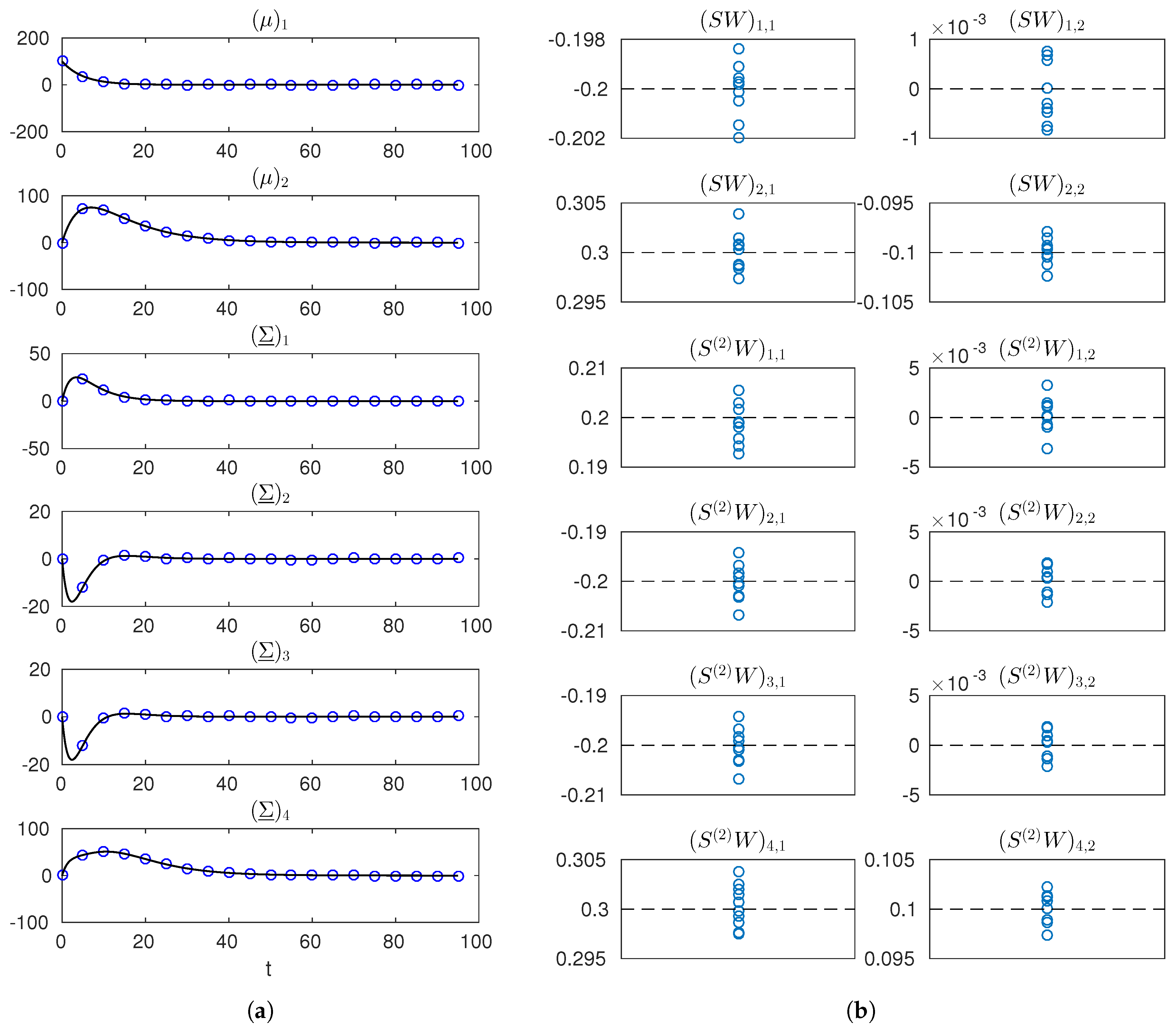
Finally, for Case (ii), we implemented and run the full identification procedure of Section 4.3 from simulated data. Here, the products $S^{\ast }{W}^{\ast }$ and ${\left(S^{\ast }\right)}^{\left(2\right)}{W}^{\ast }$ are not known and are estimated from noisy mean and variance measurements. These measurements were obtained by simulating the moment Equations (10) and (11) with the true $S^{\ast }$ and $W^{\ast }$ from initial conditions known and fixed to $\mu \left(0\right)={[100,0]}^T$ and $\Sigma \left(0\right)$ null. We generated measurements at times $t_{\ell }=(\ell -1)·T$, with $\ell =1,\dots ,N_y$, where $T=5$ and $N_y=20$, adding random noise with covariance matrix $R_{\ell }=\mathrm{diag}({0.3}^2,{0.3}^2)$ for all ℓ, corresponding to roughly $1\%$ error on the observed mean and variance profiles. An example simulated dataset is shown in Figure 3a. The numerical optimization in the first step of the procedure, yielding noisy estimates of the matrix products $S^{\ast }{W}^{\ast }$ and ${\left(S^{\ast }\right)}^{\left(2\right)}{W}^{\ast }$, was implemented by Matlab’s lsqnonlin. Results are illustrated in Figure 3b. Estimates are found to be well-centered and little dispersed relative to the true values of the entries of $S^{\ast }{W}^{\ast }$ and ${\left(S^{\ast }\right)}^{\left(2\right)}{W}^{\ast }$, showing the effectiveness of the reconstruction of the moment dynamics. Starting from the noisy estimates of $S^{\ast }{W}^{\ast }$ and ${\left(S^{\ast }\right)}^{\left(2\right)}{W}^{\ast }$, the second step was implemented as described in Section 4.3, for a significance level of $\alpha =0.05\%$. With this noise and significance levels, for $m\in \{1,2,3,4\}$, the same solutions as in Table 1 were returned over several runs, showing feasibility and effectiveness of the approach. For the case of $m=m^{\ast }$, in particular, we quantified the rate of rejection of correct candidate solutions. Over a few hundred runs, we found this rate to be around $1\%$, that is, smaller than the prescribed rate $\alpha$. This can be ascribed to the linear approximations made to establish the ${\chi }^2$ statistic in Section 3.2. On the other hand, incorrect solutions were never accepted.

To sum up, we showed that stochastic information about the network dynamics allows one to identify the structure of a biochemical reaction network in cases where the sole mean data does not. In addition, in the scenario where the observable moments provide full information for network reconstruction, we showed that our two-step procedure is capable of correctly identifying the example network from data with realistic measurement error levels.

5. Discussion

In this paper, we have investigated the problems of parameter identification and reconstruction of interactions in biochemical reaction networks. In the context of population snapshot data (first- and second-order statistics), and state-affine reaction rates, we have provided practical methods to study identifiability of unknown parameters and algorithms to address network reconstruction. In both cases, we have shown superiority of stochastic, single-cell approaches over deterministic, population-average data. In so doing, we have also extended the existing results on identifiability of gene expression models.

Our parameter identifiability analysis is developed with reference to a given observation model (what statistics of what species are detected) and a given perturbation input. A desirable theoretical advance of our work is the investigation of identifiability as a property independent of a specific input choice. From a practical standpoint, instead, evaluating structural and practical identifiability for different inputs and observation models allows one to design most informative experiments and, for synthetic biology, the engineering of most informative intracellular reporters. Developments of our work in the context of optimal experiment design indeed constitute a first important direction of future investigation.

Our results were developed for a class of problems of immediate relevance to applications. Population-snapshot data are nowaday easily collected by simple experiments such as flow-cytometry. More complex experimental setup, such as microfuidics in combination with video-microscopy, also provide this type of data. In addition, these allow for time-lapse monitoring of individual cells, providing time correlations that we did not account for here. However, this requires nontrivial processing of raw images entailing single-cell tracking procedures, which are not always performed in practice. Instead, for network reconstruction, more complex measurement scenarios, such as the monitoring of a subset of the network species and lack of covariance measurements across different species, shall be addressed in detail to widen the applicability of our methods.

Of course, the choice of networks with affine rates formally restricts one to reactions of zeroth- or first-order only. However, as the random-telegraph reporter gene model exemplifies, real systems of interest exist in this form. At the same time, state-affine rates have been used to model and investigate interactions of arbitrarily complex networks in an approximate manner [15]. Precise account of nonlinear stochastic dynamics instead requires generalization of our methods, for instance, with moment-closure approaches [29,42,43]. This is another direction of research.

Finally, the proposed network reconstruction methods were shown to be viable for a small toy example. Whereas automated reconstruction of small networks is of practical interest, network reconstruction methods are of greatest help for the investigation of larger networks of interactions. Our current algorithm performs fast on small networks but scales poorly with the network size (number of species and putative reaction channels). As anticipated in Section 4.2, great improvements can be easily obtained by an optimized implementation that avoids the exploration of redundant network candidates. In particular, considering that not only permutations of the reactions list but also identical columns of a stoichiometry matrix are redundant, it can be seen that the number of effectively distinct stoichiometry matrices to be tested is in the order of $\left(\genfrac{}{}{0pt}{}{S_{max}^n}{m}\right)$. Therefore, an optimized implementation of the method would reduce complexity from $\mathcal{O}(S_{max}^{nm})$ to $\mathcal{O}\left((,\genfrac{}{}{0pt}{}{S_{max}^n}{m},)\right)$. However, the discrete nature of the stoichiometry matrix makes the problem inevitably hard, and advanced mixed-integer programming methods should be explored in order to tackle the exponential growth of complexity with the network size. This is yet another research direction of practical relevance.

References

- Ashyraliyev, M.; Fomekong-Nanfack, Y.; Kaandorp, J.; Blom, J. Systems Biology: Parameter Estimation for Biochemical Models. FEBS J. 2009, 276, 886–902. [Google Scholar] [CrossRef] [PubMed]
- Marbach, D.; Costello, J.; Küffner, R.; Vega, N.; Prill, R.; Camacho, D.; Allison, K.; The DREAM5 Consortium; Kellis, M.; Collins, J.; et al. Wisdom of crowds for robust gene network inference. Nat. Methods 2012, 9, 796–804. [Google Scholar] [CrossRef] [PubMed] [Green Version]
- Purnick, P.; Weiss, R. The second wave of synthetic biology: From modules to systems. Nat. Rev. Mol. Cell Biol. 2009, 10, 410–422. [Google Scholar] [CrossRef] [PubMed]
- Chis, O.T.; Banga, J.R.; Balsa-Canto, E. Structural Identifiability of Systems Biology Models: A Critical Comparison of Methods. PLoS ONE 2011, 6, e27755. [Google Scholar] [CrossRef] [PubMed] [Green Version]
- Gutenkunst, R.N.; Waterfall, J.J.; Casey, F.P.; Brown, K.S.; Myers, C.R.; Sethna, J.P. Universally Sloppy Parameter Sensitivities in Systems Biology Models. PLoS Comput. Biol. 2007, 3, e189. [Google Scholar] [CrossRef] [PubMed] [Green Version]
- Raue, A.; Kreutz, C.; Maiwald, T.; Bachmann, J.; Schilling, M.; Klingmüller, U.; Timmer, J. Structural and practical identifiability analysis of partially observed dynamical models by exploiting the profile likelihood. Bioinformatics 2009, 25, 1923–1929. [Google Scholar] [CrossRef] [PubMed] [Green Version]
- Taniguchi, Y.; Choi, P.J.; Li, G.W.; Chen, H.; Babu, M.; Hearn, J.; Emili, A.; Xie, X.S. Quantifying E. coli proteome and transcriptome with single-molecule sensitivity in single cells. Science 2010, 329, 533–538. [Google Scholar] [CrossRef] [PubMed]
- Munsky, B.; Trinh, B.; Khammash, M. Listening to the noise: Random fluctuations reveal gene network parameters. Mol. Syst. Biol. 2009, 5, 318. [Google Scholar] [CrossRef] [PubMed]
- Zechner, C.; Ruess, J.; Krenn, P.; Pelet, S.; Peter, M.; Lygeros, J.; Koeppl, H. Moment-based inference predicts bimodality in transient gene expression. PNAS 2012, 109, 8340–8345. [Google Scholar] [CrossRef] [PubMed] [Green Version]
- Helmke, U.; Hüper, K.; Khammash, M. Global identifiability of a simple linear model for gene expression analysis. In Proceedings of the 52nd IEEE CDC, Florence, Italy, 10–13 December 2013. [Google Scholar]
- Cho, K.H.; Choo, S.M.; Jung, S.; Kim, J.R.; Choi, H.S.; Kim, J. Reverse engineering of gene regulatory networks. IET Syst. Biol. 2007, 1, 149–163. [Google Scholar] [CrossRef] [PubMed]
- Markowetz, F.; Spang, R. Inferring cellular networks: A review. BMC Bioinform. 2007, 28, S5. [Google Scholar] [CrossRef] [PubMed]
- Hasenauer, J.; Waldherr, S.; Doszczak, M.; Radde, N.; Scheurich, P.; Allgower, F. Identification of models of heterogeneous cell populations from population snapshot data. BMC Bioinform. 2011, 12, 125. [Google Scholar] [CrossRef] [PubMed]
- Paulsson, J. Models of stochastic gene expression. Phys. Life Rev. 2005, 2, 157–175. [Google Scholar] [CrossRef]
- Thattai, M.; van Oudenaarden, A. Intrinsic noise in gene regulatory networks. PNAS 2001, 98, 8614–8619. [Google Scholar] [CrossRef] [PubMed] [Green Version]
- Hespanha, J. Modelling and analysis of stochastic hybrid systems. IEE Proc. Control Theory Appl. 2006, 153, 520–535. [Google Scholar] [CrossRef]
- Sotiropoulos, V.; Kaznessis, Y. Analytical Derivation of Moment Equations in Stochastic Chemical Kinetics. Chem. Eng. Sci. 2011, 66, 268–277. [Google Scholar] [CrossRef] [PubMed]
- Cinquemani, E. Reconstruction of promoter activity statistics from reporter protein population snapshot data. In Proceedings of the 54th IEEE CDC, Osaka, Japan, 15–18 December 2015; pp. 1471–1476. [Google Scholar]
- Cinquemani, E. Structural identification of biochemical reaction networks from population snapshot data. In Proceedings of the 20th IFAC World Congress, IFAC—PapersOnLine, Toulouse, France, 9–14 July 2017; Volume 50, pp. 12629–12634. [Google Scholar]
- Berthoumieux, S.; Brilli, M.; Kahn, D.; de Jong, H.; Cinquemani, E. On the identifiability of metabolic network models. J. Math. Biol. 2013, 67, 1795–1832. [Google Scholar] [CrossRef] [PubMed]
- Bansal, M.; Belcastro, V.; Ambesi-Impiombato, A.; di Bernardo, D. How to infer gene networks from expression profiles. Mol. Syst. Biol. 2007, 3, 78. [Google Scholar] [CrossRef] [PubMed]
- Gardner, T.; Faith, J. Reverse-engineering transcription control networks. Phys. Life Rev. 2005, 2, 65–88. [Google Scholar] [CrossRef] [PubMed]
- Porreca, R.; Cinquemani, E.; Lygeros, J.; Ferrari-Trecate, G. Identification of genetic network dynamics with unate structure. Bioinformatics 2010, 26, 1239–1245. [Google Scholar] [CrossRef] [PubMed] [Green Version]
- Neuert, G.; Munsky, B.; Tan, R.; Teytelman, L.; Khammash, M.; van Oudenaarden, A. Systematic Identification of Signal-Activated Stochastic Gene Regulation. Science 2013, 339, 584–587. [Google Scholar] [CrossRef] [PubMed] [Green Version]
- Gillespie, D. A Rigorous Derivation of the Chemical Master Equation. Physica A 1992, 188, 404–425. [Google Scholar] [CrossRef]
- Van Kampen, N. Stochastic Processes in Physics and Chemistry; North-Holland Personal Library: Amsterdam, The Netherlands, 1992. [Google Scholar]
- Gadgil, C.; Lee, C.; Othmer, H. A stochastic analysis of first-order reaction networks. Bull. Math. Biol. 2005, 67, 901–946. [Google Scholar] [CrossRef] [PubMed] [Green Version]
- Gillespie, D.T. The chemical Langevin equation. J. Chem. Phys. 2000, 113, 297–306. [Google Scholar] [CrossRef] [Green Version]
- Gillespie, C. Moment-closure approximations for mass-action models. IET Syst. Biol. 2009, 3, 52–58. [Google Scholar] [CrossRef] [PubMed]
- Parise, F.; Ruess, J.; Lygeros, J. Grey-box techniques for the identification of a controlled gene expression model. In Proceedings of the ECC, Strasbourg, France, 24–27 June 2014. [Google Scholar]
- Walter, E.; Pronzato, L. Identification of Parametric Models—From Experimental Data; Springer: London, UK, 1997. [Google Scholar]
- Walter, E. (Ed.) Identifiability of Parametric Models; Pergamon Press: Oxford, UK, 1987. [Google Scholar]
- Khalil, H.K. Nonlinear Systems; Prentice Hall: Upper Saddle River, NJ, USA, 2002. [Google Scholar]
- Ruess, J.; Lygeros, J. Identifying stochastic biochemical networks from single-cell population experiments: A comparison of approaches based on the Fisher information. In Proceedings of the 52nd IEEE CDC, Florence, Italy, 10–13 December 2013; pp. 2703–2708. [Google Scholar]
- Kay, S.M. Fundamentals of Statistical Signal Processing [Volume I] Estimation Theory; Prentice Hall: Upper Saddle River, NJ, USA, 1993; p. 1. [Google Scholar]
- De Jong, H.; Ranquet, C.; Ropers, D.; Pinel, C.; Geiselmann, J. Experimental and computational validation of models of fluorescent and luminescent reporter genes in bacteria. BMC Syst. Biol. 2010, 4, 55. [Google Scholar] [CrossRef] [PubMed]
- Kaern, M.; Elston, T.C.; Blake, W.J.; Collins, J.J. Stochasticity in gene expression: From theories to phenotypes. Nat. Rev. Gen. 2005, 6, 451–464. [Google Scholar] [CrossRef] [PubMed]
- Sanft, K.R.; Wu, S.; Roh, M.; Fu, J.; Lim, R.K.; Petzold, L.R. StochKit2: Software for discrete stochastic simulation of biochemical systems with events. Bioinformatics 2011, 27, 2457–2458. [Google Scholar] [CrossRef] [PubMed]
- Ljung, L. System Identification: Theory for the User; Prentice Hall: Upper Saddle River, NJ, USA, 1999. [Google Scholar]
- Callier, F.; Desoer, C. Linear System Theory; Springer: New York, NY, USA, 1991. [Google Scholar]
- Boyd, S.; Vandenberghe, L. Convex Optimization; Cambridge University Press: New York, NY, USA, 2004. [Google Scholar]
- Singh, A.; Hespanha, J. Approximate Moment Dynamics for Chemically Reacting Systems. IEEE Trans. Autom. Control 2011, 56, 414–418. [Google Scholar] [CrossRef] [Green Version]
- Ruess, J.; Milias-Argeitis, A.; Summers, S.; Lygeros, J. Moment estimation for chemically reacting systems by extended Kalman filtering. J. Chem. Phys. 2011, 135, 165102. [Google Scholar] [CrossRef] [PubMed]
Figure 1.
Reporter gene system. The coding sequence of a fluorescent reporter protein is engineered into a gene of interest. The gene promoter can switch between an inactive (off) and an active (on) state. When active, transcription of reporter mRNA molecules is enabled. Existing mRNA molecules are further translated into visible (quantifiable) reporter protein molecules. Both mRNA and protein molecules are subject to degradation.
Figure 2.
Parameter estimation results. (a) scatter plots of the estimates of parameters from 10 simulated datasets (blue dots) and theoretically computed confidence regions (red lines). Results for all different pairs of these parameters are reported in the different boxes, as per labeling on top and left of the figure. Estimated values and pairwise confidence ellipsoids (one-dimensional confidence intervals for boxes on the diagonal) are normalized by the true parameter values. Dashed lines show the reference coordinates corresponding to true values; (b) estimated dynamics of the system means (left) and variances (right), corresponding to the 10 different estimates of in (a). Solid blue lines show estimates, dashed black lines show true system statistics. In the bottom plots, black circles show measurements used for one of these estimates.
Figure 3.
Simulated measurements and estimates of and for the network reconstruction example. (a) true trajectories of the entries of and (solid black line) and one simulated dataset (blue markers); (b) estimates of the entries of and (blue markers) obtained from 10 different datasets (dashed black lines indicate true values). Notation is used in labels to denote the row-r, column-c entry of a matrix.