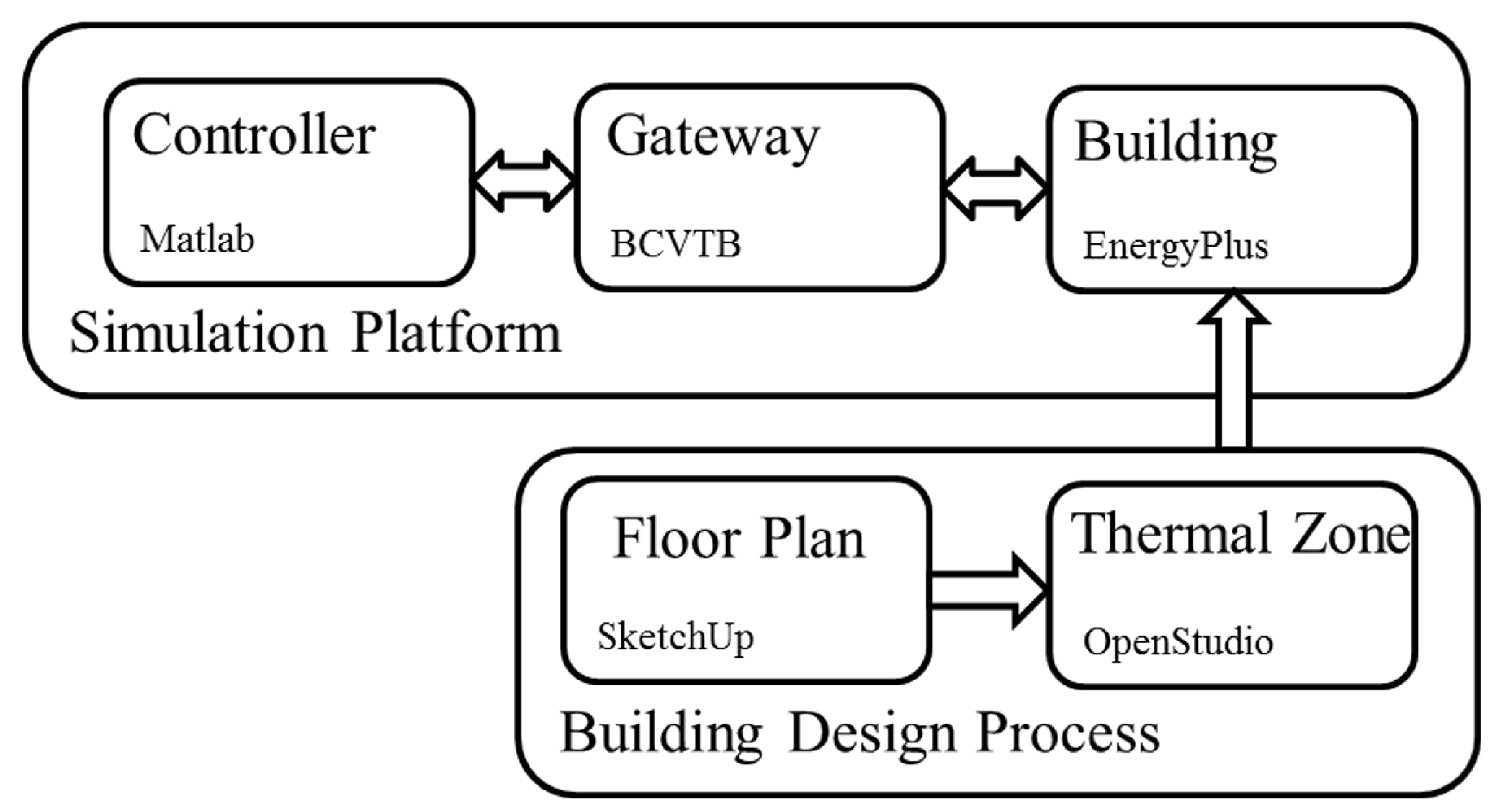
Figure 1.
A conceptual flow diagram showing the entire simulation platform design process, including the building design step, as well as the control simulation platform step.
Figure 1.
A conceptual flow diagram showing the entire simulation platform design process, including the building design step, as well as the control simulation platform step.
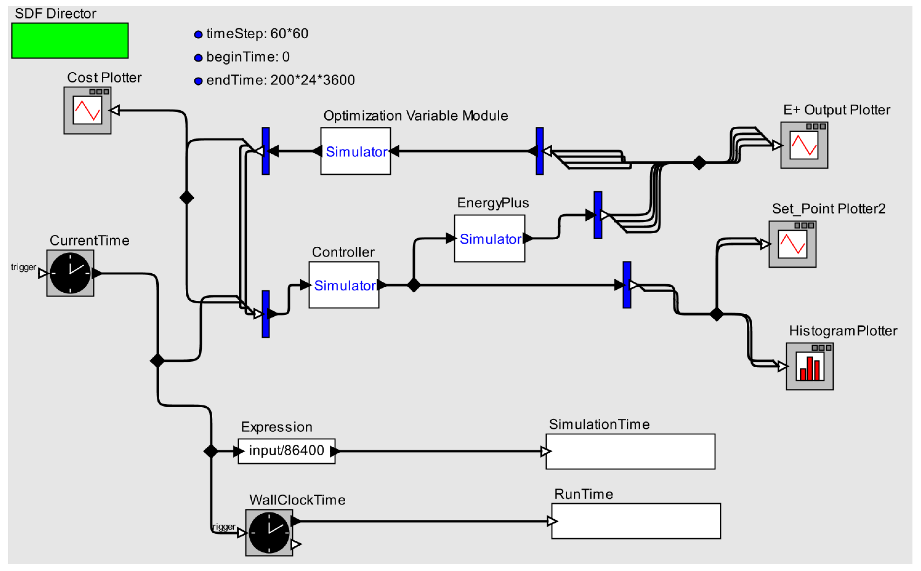
Figure 2.
An overview of the BCVTB building simulation setup. It shows three modules (optimization variable, EnergyPlus and controller) alongside various ancillary plotting, time-keeping functionalities. In the figure, blue bars are for splitting output vector streams into multi-line data streams for plotting and data saving uses.
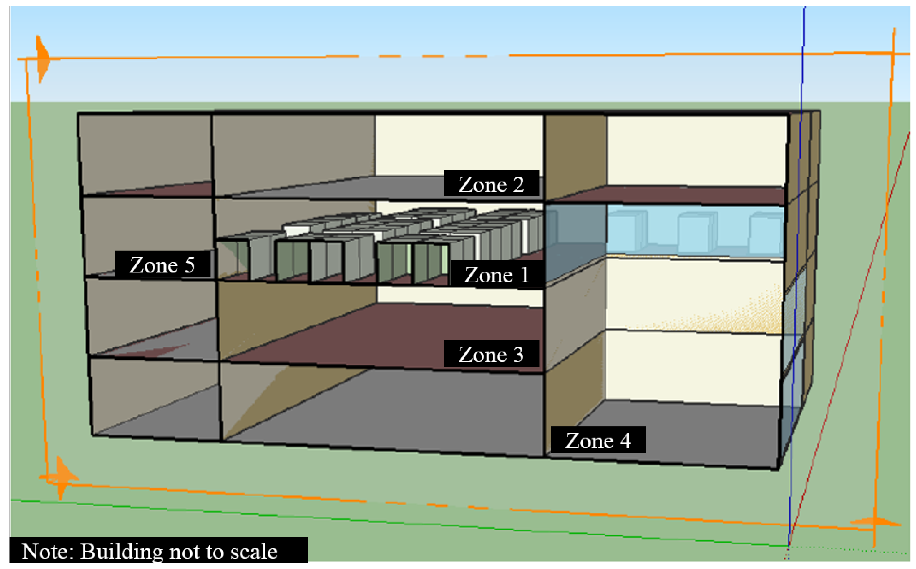
Figure 3.
3D model of our simulated office building zone in SketchUp. Zone 1 is the simulated zone, with Zones 2–5 acting as adjacent, ideal air zones.
Figure 3.
3D model of our simulated office building zone in SketchUp. Zone 1 is the simulated zone, with Zones 2–5 acting as adjacent, ideal air zones.
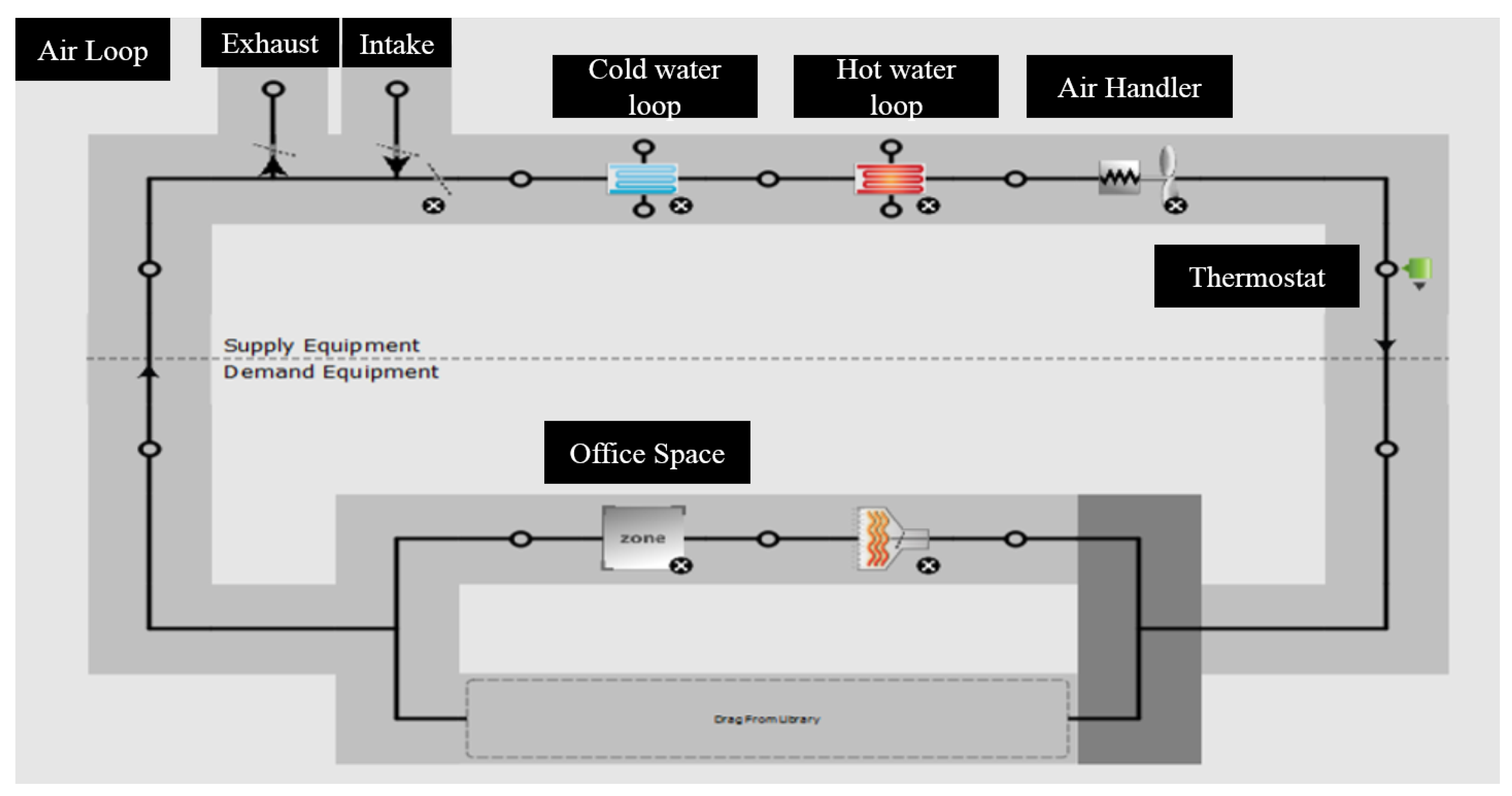
Figure 4.
Layout of the simple Variable Air Volume (VAV) HVAC Loop implemented within our room zone simulation. This was a plug-and-use (VAV) module available when designing the building in SketchUp.
Figure 4.
Layout of the simple Variable Air Volume (VAV) HVAC Loop implemented within our room zone simulation. This was a plug-and-use (VAV) module available when designing the building in SketchUp.
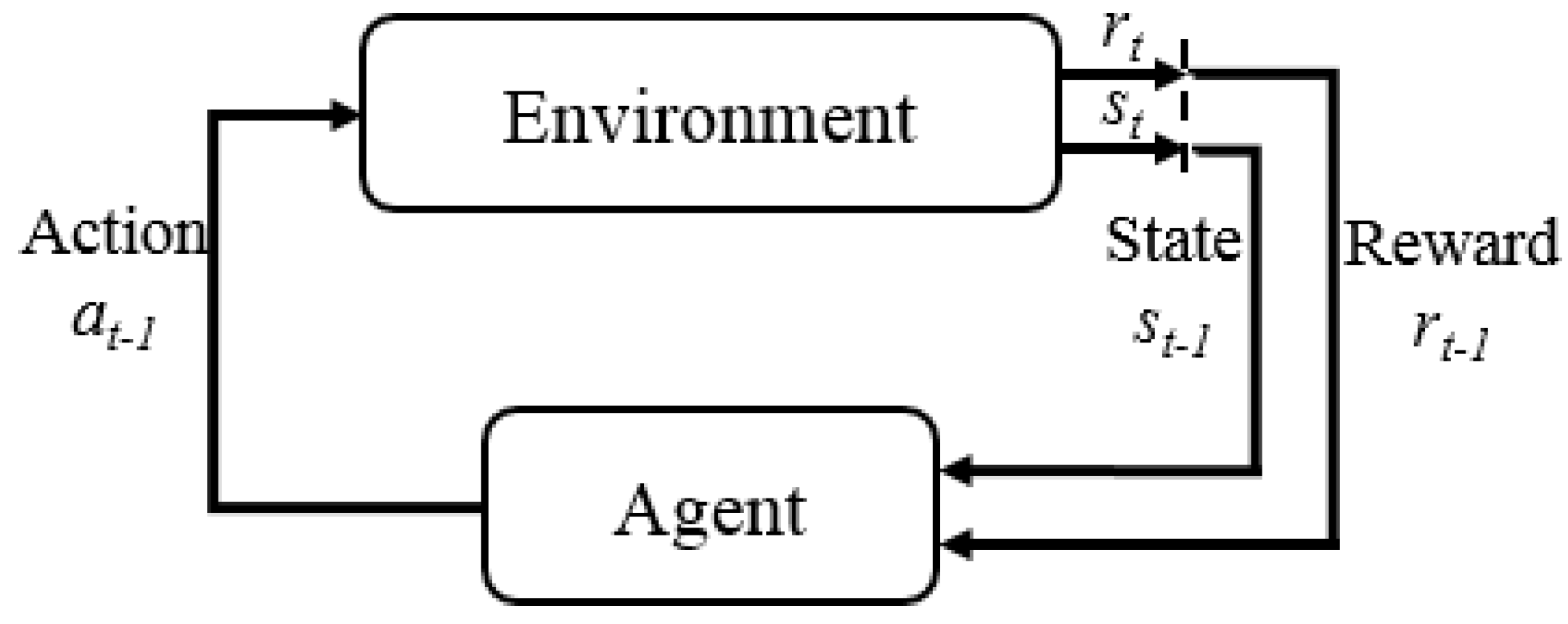
Figure 5.
A figure showing the various components in a reinforcement learning problem setting. The dashed vertical line indicates a transition in discrete time/sequence. This diagram shows a full transition in states and reward from one time step to the next.
Figure 5.
A figure showing the various components in a reinforcement learning problem setting. The dashed vertical line indicates a transition in discrete time/sequence. This diagram shows a full transition in states and reward from one time step to the next.
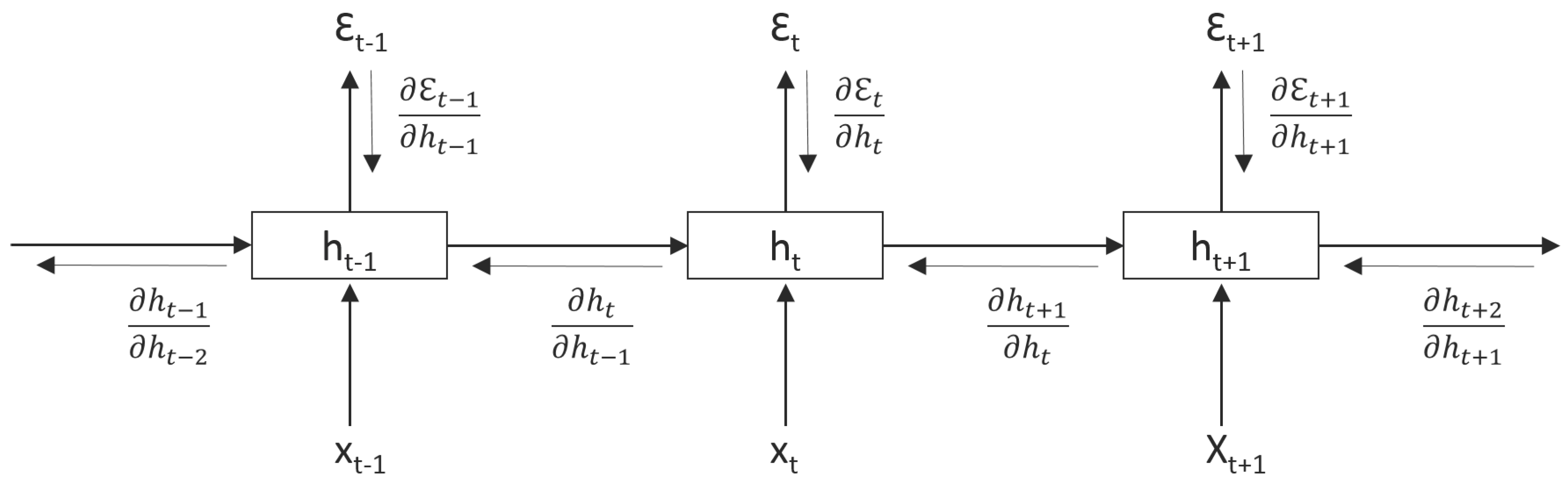
Figure 6.
The RNN here has been unrolled for three time steps for some arbitrary sequential data. At every time step, the RNN’s output is computed, as well as the hidden state is passed forward through time. During back-propagation, the gradients flow back in two paths; first from error outputs at every time step , as well as the gradient back-flow through time through the recurrent states, .
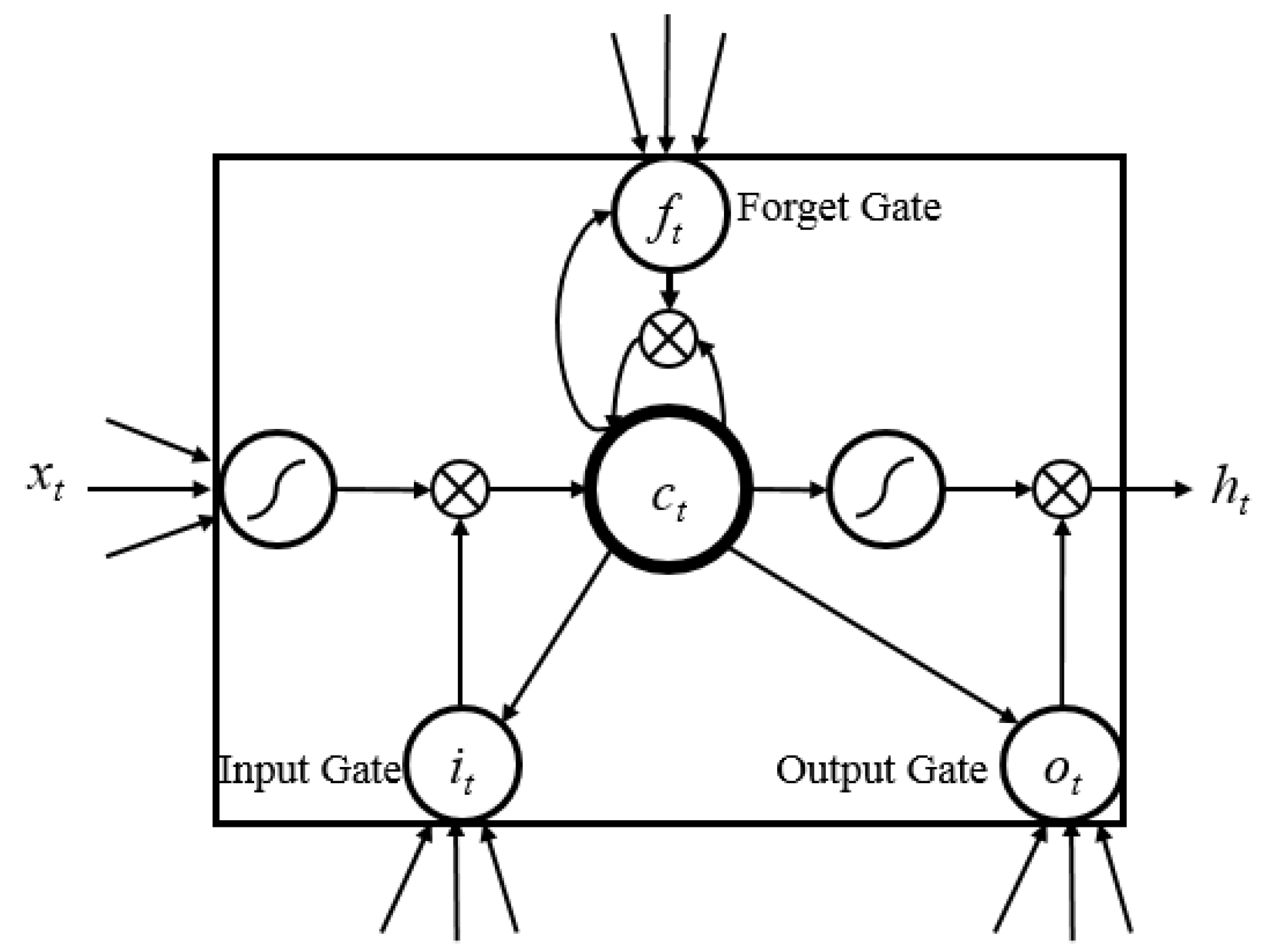
Figure 7.
A visual diagram of the LSTM architecture, showing the input, forget and output gates, as well as the cell state computation and updates.
Figure 7.
A visual diagram of the LSTM architecture, showing the input, forget and output gates, as well as the cell state computation and updates.
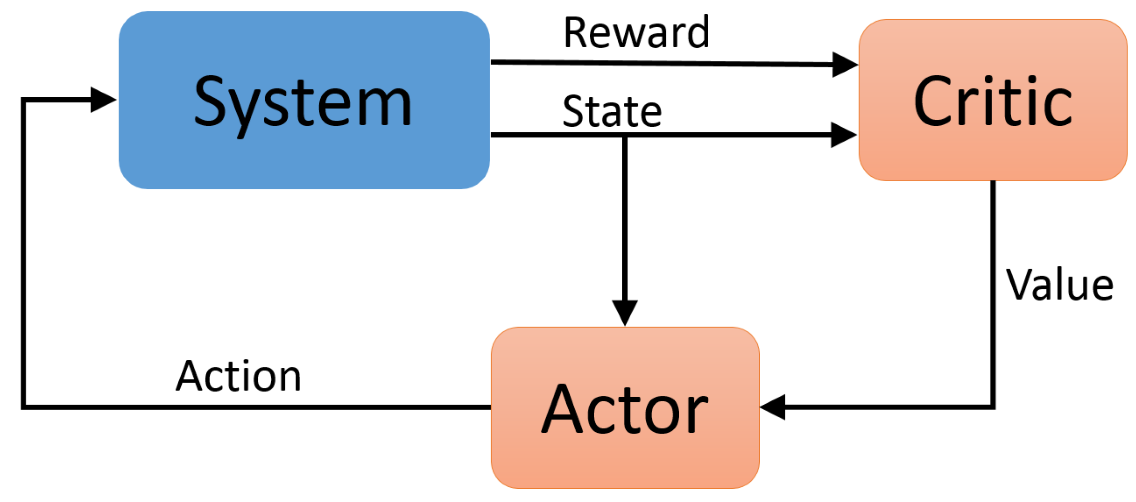
Figure 8.
A high-level block diagram of the actor-critic reinforcement learning architecture is shown. This shows the general flow of state observations and reward signals between the algorithm and the environment, the critic’s update and its value estimate, which is used by the policy in it’s policy gradient updates.
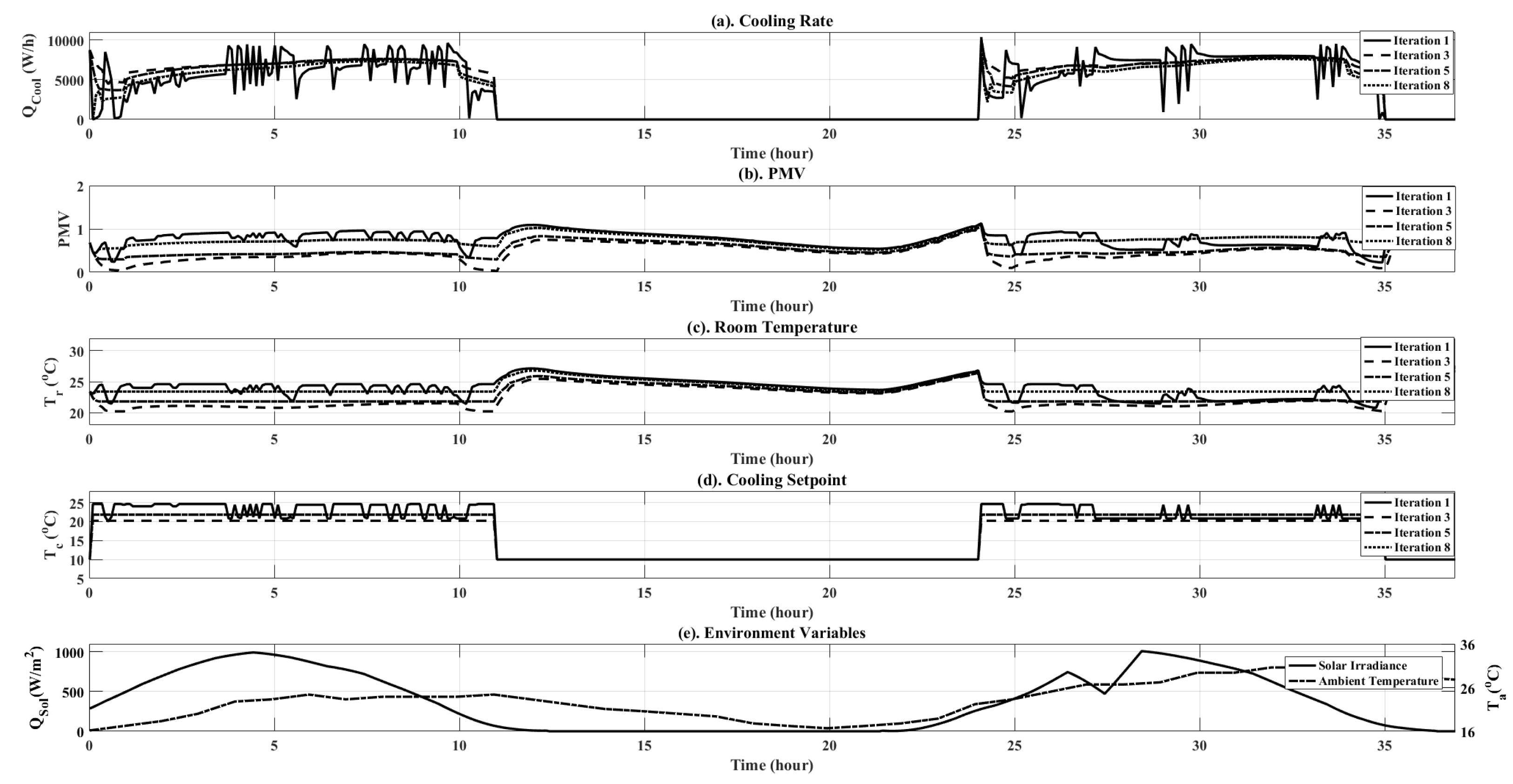
Figure 9.
Simulation results plots for the RL controller at various iterations of training. Plots are shown for both objective variables ( and PMV), as well as additional simulation data, such as ambient temperature and solar irradiance.
Figure 9.
Simulation results plots for the RL controller at various iterations of training. Plots are shown for both objective variables ( and PMV), as well as additional simulation data, such as ambient temperature and solar irradiance.
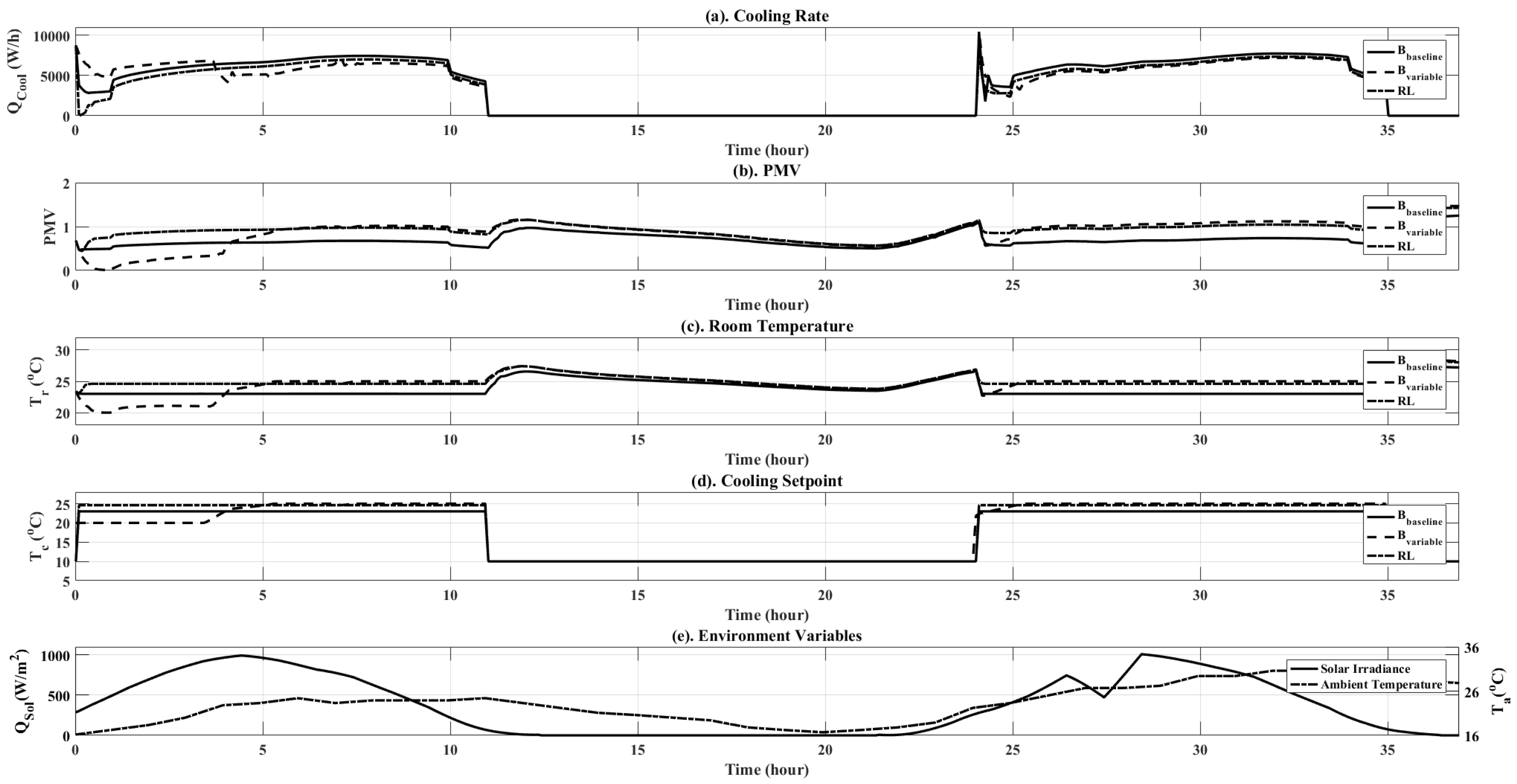
Figure 10.
Simulation results plots for comparison between , and the RL controller over two days. Plots are shown for both objective variables ( and PMV), as well as additional simulation data, such as ambient temperature and solar irradiance.
Figure 10.
Simulation results plots for comparison between , and the RL controller over two days. Plots are shown for both objective variables ( and PMV), as well as additional simulation data, such as ambient temperature and solar irradiance.
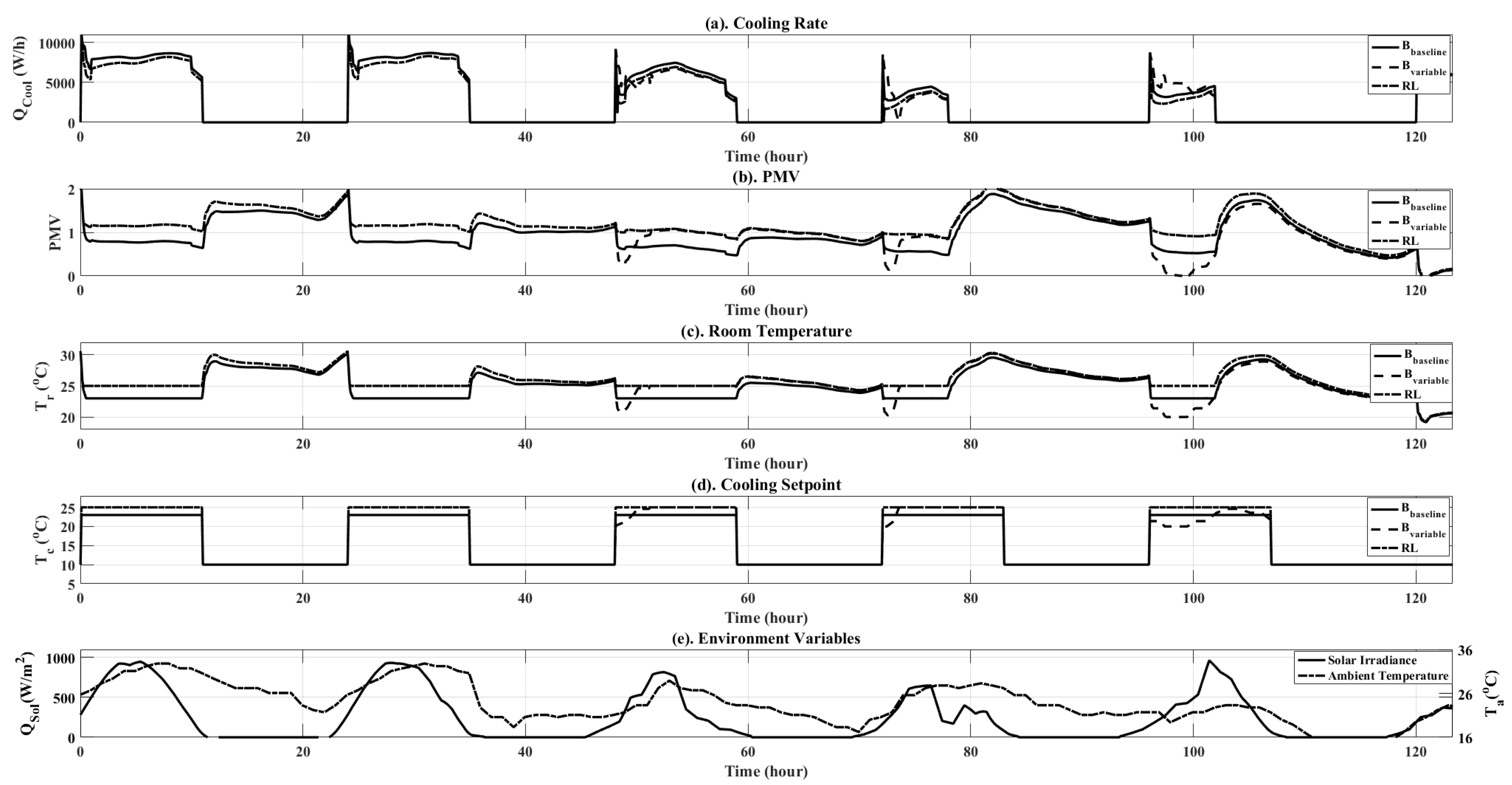
Figure 11.
Simulation results plots for comparison between , and the RL controller over the five-day validation runs. Plots are shown for both objective variables ( and PMV), as well as additional simulation data, such as ambient temperature and solar irradiance.
Figure 11.
Simulation results plots for comparison between , and the RL controller over the five-day validation runs. Plots are shown for both objective variables ( and PMV), as well as additional simulation data, such as ambient temperature and solar irradiance.
Table 1.
This table provides the daily occupancy schedule for a typical work day on an hourly-basis. Values reported in fractions. This occupancy schedule was used in our simulation.
Table 1.
This table provides the daily occupancy schedule for a typical work day on an hourly-basis. Values reported in fractions. This occupancy schedule was used in our simulation.
| Hours | Office Occupancy | Equipment Active Schedule |
|---|
| 01:00 a.m. | 0 | 0 |
| 02:00 a.m. | 0 | 0 |
| 03:00 a.m. | 0 | 0 |
| 04:00 a.m. | 0 | 0 |
| 05:00 a.m. | 0 | 0 |
| 06:00 a.m. | 0 | 0 |
| 07:00 a.m. | 0.5 | 1 |
| 08:00 a.m. | 1.0 | 1 |
| 09:00 a.m. | 1.0 | 1 |
| 10:00 a.m. | 1.0 | 1 |
| 11:00 a.m. | 1.0 | 1 |
| 12:00 p.m. | 0.5 | 1 |
| 01:00 p.m. | 1.0 | 1 |
| 02:00 p.m. | 1.0 | 1 |
| 03:00 p.m. | 1.0 | 1 |
| 04:00 p.m. | 1.0 | 1 |
| 05:00 p.m. | 0.5 | 1 |
| 06:00 p.m. | 0.1 | 1 |
| 07:00 p.m. | 0 | 0 |
| 08:00 p.m. | 0 | 0 |
| 09:00 p.m. | 0 | 0 |
| 10:00 p.m. | 0 | 0 |
| 11:00 p.m. | 0 | 0 |
| 12:00 a.m. | 0 | 0 |
Table 2.
RL training results.
Table 2.
RL training results.
| Iteration Number | PMV Total (Unitless) | Energy Total (W) | Standard Deviation ( W/h) |
|---|
| 1 | 216.70 | 16,717 | 3580 |
| 2 | 113.50 | 18,079 | 3480 |
| 3 | 105.60 | 18,251 | 3500 |
| 4 | 262.00 | 15,398 | 3070 |
| 5 | 132.12 | 17,698 | 3450 |
| 6 | 211.30 | 16,300 | 3240 |
| 7 | 211.50 | 16,310 | 3240 |
| 8 | 211.30 | 16,298 | 3228 |
Table 3.
Training comparison.
Table 3.
Training comparison.
| Control Type | PMV (Unitless) | Energy Total (W) |
|---|
| Ideal PMV | 190.00 | 16,676 |
| Variable Control | 250.00 | 15,467 |
| RL Control | 211.3 | 16,298 |
Table 4.
Validation comparison over 5 simulation days.
Table 4.
Validation comparison over 5 simulation days.
| Control Type | PMV Total (Unitless) | Energy Total (W) |
|---|
| Ideal PMV | 510 | 42,094 |
| Variable Control | 660 | 38,536 |
| RL Control | 558 | 39,978 |


