Sensitivity-Based Economic NMPC with a Path-Following Approach

Abstract

We present a sensitivity-based predictor-corrector path-following algorithm for fast nonlinear model predictive control (NMPC) and demonstrate it on a large case study with an economic cost function. The path-following method is applied within the advanced-step NMPC framework to obtain fast and accurate approximate solutions of the NMPC problem. In our approach, we solve a sequence of quadratic programs to trace the optimal NMPC solution along a parameter change. A distinguishing feature of the path-following algorithm in this paper is that the strongly-active inequality constraints are included as equality constraints in the quadratic programs, while the weakly-active constraints are left as inequalities. This leads to close tracking of the optimal solution. The approach is applied to an economic NMPC case study consisting of a process with a reactor, a distillation column and a recycler. We compare the path-following NMPC solution with an ideal NMPC solution, which is obtained by solving the full nonlinear programming problem. Our simulations show that the proposed algorithm effectively traces the exact solution.

1. Introduction

The idea of economic model predictive control (MPC) is to integrate the economic optimization layer and the control layer in the process control hierarchy into a single dynamic optimization layer. While classic model predictive control approaches typically employ a quadratic objective to minimize the error between the setpoints and selected measurements, economic MPC adjusts the inputs to minimize the economic cost of operation directly. This makes it possible to optimize the cost during transient operation of the plant. In recent years, this has become increasingly desirable, as stronger competition, volatile energy prices and rapidly changing product specifications require agile plant operations, where also transients are optimized to maximize profit.

The first industrial implementations of economic MPC were reported in [1,2] for oil refinery applications. The development of theory and stability analysis for economic MPC arose almost a decade afterwards; see, e.g., [3,4]. Recent progress on economic MPC is reviewed and surveyed in [5,6]. Most of the current research activities focus on the stability analysis of economic MPC and do not discuss its performance (an exception is [7]).

Because nonlinear process models are often used for economic optimization, a potential drawback of economic MPC is that it requires solving a large-scale nonlinear optimization problem (NLP) associated with the nonlinear model predictive control (NMPC) problem at every sample time. The solution of this NLP may take a significant amount of time [8], and this can lead to performance degradation and even to instability of the closed-loop system [9].

To reduce the detrimental effect of computational delay in NMPC, several sensitivity-based methods were proposed [10,11,12]. All of these fast sensitivity approaches exploit the fact that the NMPC optimization problems are identical at each sample time, except for one varying parameter: the initial state. Instead of solving the full nonlinear optimization problem when new measurements of the state become available, these approaches use the sensitivity of the NLP solution at a previously-computed iteration to obtain fast approximate solutions to the new NMPC problem. These approximate solutions can be computed and implemented in the plant with minimal delay. A recent overview of the developments in fast sensitivity-based nonlinear MPC is given in [13], and a comparison of different approaches to obtain sensitivity updates for NMPC is compiled in the paper by Wolf and Marquardt [14].

Diehl et al. [15] proposed the concept of real-time iteration (RTI), in which the full NLP is not solved at all during the MPC iterations. Instead, at each NMPC sampling time, a single quadratic programming (QP) related to the sequential quadratic programming (SQP) iteration for solving the full NLP is solved. The real-time iteration scheme contains two phases: (1) the preparation phase and (2) the feedback phase. In the preparation phase, the model derivatives are evaluated using a predicted state measurement, and a QP is formulated based on data of this predicted state. In the feedback phase, once the new initial state is available, the QP is updated to include the new initial state and solved for the control input that is injected into the plant. The real-time iteration scheme has been applied to economic NMPC in the context of wind turbine control [16,17]. Similar to the real-time iteration scheme are the approaches by Ohtsuka [18] and the early paper by Li and Biegler [19], where one single Newton-like iteration is performed per sampling time.

A different approach, the advanced-step NMPC (asNMPC), was proposed by Zavala and Biegler [10]. The asNMPC approach involves solving the full NLP at every sample time. However, the full NLP solution is computed in advance for a predicted initial state. Once the new state measurement is available, the NLP solution is corrected using a fast sensitivity update to match the measured or estimated initial state. A simple sensitivity update scheme is implemented in the software package sIPOPT [20]. However, active set changes are handled rather heuristically; see [21] for an overview. Kadam and Marquardt [22] proposed a similar approach, where nominal NLP solutions are updated by solving QPs in a neighboring extremal scheme; see also [12,23].

The framework of asNMPC was also applied by Jäschke and Biegler [24], who use a multiple-step predictor path-following algorithm to correct the NLP predictions. Their approach included measures to handle active set changes rigorously, and their path-following advanced-step NMPC algorithm is also the first one to handle non-unique Lagrange multipliers.

The contribution of this paper is to apply an improved path-following method for correcting the NLP solution within the advanced-step NMPC framework. In particular, we replace the predictor path-following method from [24] by a predictor-corrector method and demonstrate numerically that the method works efficiently on a large-scale case study. We present how the asNMPC with the predictor-corrector path-following algorithm performs in the presence of measurement noise and compare it with a pure predictor path-following asNMPC approach and an ideal NMPC approach, where the NLP is assumed to be solved instantly. We also give a brief discussion about how our method differs from previously published approaches.

The structure of this paper is the following. We start by introducing the ideal NMPC and advanced-step NMPC frameworks in Section 2 and give a description of our path-following algorithm together with some relevant background material and a brief discussion in Section 3. The proposed algorithm is applied to a process with a reactor, distillation and recycling in Section 4, where we consider the cases with and without measurement noise and discuss the results. The paper is closed with our conclusions in Section 5.

2. NMPC Problem Formulations

2.1. The NMPC Problem

We consider a nonlinear discrete-time dynamic system:

$$\begin{array}{cc}\hfill {\mathbf{x}}_{k+1}& =f\left({\mathbf{x}}_k,{\mathbf{u}}_k\right)\end{array}$$

(1)

where ${\mathbf{x}}_k\in {\mathbb{R}}^{n_x}$ denotes the state variable, ${\mathbf{u}}_k\in {\mathbb{R}}^{n_u}$ is the control input and $f:{\mathbb{R}}^{n_x}\times {\mathbb{R}}^{n_u}\to {\mathbb{R}}^{n_x}$ is a continuous model function, which calculates the next state ${\mathbf{x}}_{k+1}$ from the previous state ${\mathbf{x}}_k$ and control input ${\mathbf{u}}_k$, where $k\in \mathbb{N}$. This system is optimized by a nonlinear model predictive controller, which solves the problem:

$$\begin{array}{ccc}\hfill \left({\mathcal{P}}_{nmpc}\right):& \underset{{\mathbf{z}}_l,{\mathbf{v}}_l}{\min }& \Psi \left({\mathbf{z}}_N\right)+\sum _{l=0}^{N-1}\psi ({\mathbf{z}}_l,{\mathbf{v}}_l)\hfill \\ \hfill \mathrm{s}.\mathrm{t}.& {\mathbf{z}}_{l+1}=f({\mathbf{z}}_l,{\mathbf{v}}_l)& l=0,\dots ,N-1,\hfill \\ & {\mathbf{z}}_0={\mathbf{x}}_k,& \\ & \left({\mathbf{z}}_l,{\mathbf{v}}_l\right)\in \mathcal{Z},& l=0,\dots ,N-1,\hfill \\ & {\mathbf{z}}_N\in {\mathcal{X}}_f,& \end{array}$$

(2)

at each sample time. Here, ${\mathbf{z}}_l\in {\mathbb{R}}^{n_x}$ is the predicted state variable; ${\mathbf{v}}_l\in {\mathbb{R}}^{n_u}$ is the predicted control input; and ${\mathbf{z}}_N\in {\mathcal{X}}_f$ is the final predicted state variable restricted to the terminal region ${\mathcal{X}}_f\in {\mathbb{R}}^{n_x}$. The stage cost is denoted by $\psi :{\mathbb{R}}^{n_x}\times {\mathbb{R}}^{n_u}\to \mathbb{R}$ and the terminal cost by $\Psi :{\mathcal{X}}_f\to \mathbb{R}$. Further, $\mathcal{Z}$ denotes the path constraints, i.e., $\mathcal{Z}=\left\{\left(\mathbf{z},\mathbf{v}\right)\mid q\left(\mathbf{z},\mathbf{v}\right)\le 0\right\}$, where $q:{\mathbb{R}}^{n_x}\times {\mathbb{R}}^{n_u}\to {\mathbb{R}}^{n_q}$.

The solution of the optimization problem ${\mathcal{P}}_{nmpc}$ is denoted $\left\{{\mathbf{z}}_0^{*},\dots ,{\mathbf{z}}_N^{*},{\mathbf{v}}_0^{*},\dots ,{\mathbf{v}}_{N-1}^{*}\right\}$. At sample time k, an estimate or measurement of the state ${\mathbf{x}}_k$ is obtained, and problem ${\mathcal{P}}_{nmpc}$ is solved. Then, the first part of the optimal control sequence is assigned as plant input, such that ${\mathbf{u}}_k={\mathbf{v}}_0^{*}$. This first part of the solution to ${\mathcal{P}}_{nmpc}$ defines an implicit feedback law ${\mathbf{u}}_k=\kappa \left({\mathbf{x}}_k\right)$, and the system will evolve according to ${\mathbf{x}}_{k+1}=f\left({\mathbf{x}}_k,\kappa \left({\mathbf{x}}_k\right)\right)$. At the next sample time $k+1$, when the measurement of the new state ${\mathbf{x}}_{k+1}$ is obtained, the procedure is repeated. The NMPC algorithm is summarized in Algorithm 1.

Algorithm 1: General NMPC algorithm.

2.2. Ideal NMPC and Advanced-Step NMPC Framework

For achieving optimal economic performance and good stability properties, problem ${\mathcal{P}}_{nmpc}$ needs to be solved instantly, so that the optimal input can be injected without time delay as soon as the values of the new states are available. We refer to this hypothetical case without computational delay as ideal NMPC.

In practice, there will always be some time delay between obtaining the updated values of the states and injecting the updated inputs into the plant. The main reason for this delay is the time it requires to solve the optimization problem ${\mathcal{P}}_{nmpc}$. As the process models become more advanced, solving the optimization problems requires more time, and the computational delay cannot be neglected any more. This has led to the development of fast sensitivity-based NMPC approaches. One such approach that will be a adopted in this paper is the advanced-step NMPC (asNMPC) approach [10]. It is based on the following steps:

• Solve the NMPC problem at time k with a predicted state value of time $k+1$,
• When the measurement ${\mathbf{x}}_{k+1}$ becomes available at time $k+1$, compute an approximation of the NLP solution using fast sensitivity methods,
• Update $k\leftarrow k+1$, and repeat from Step 1.

Zavala and Biegler proposed a fast one-step sensitivity update that is based on solving a linear system of equations [10]. Under some assumptions, this corresponds to a first-order Taylor approximation of the optimal solution. In particular, this approach requires strict complementarity of the NLP solution, which ensures no changes in the active set. A more general approach involves allowing for changes in the active set and making several sensitivity updates. This was proposed in [24] and will be developed further in this paper.

3. Sensitivity-Based Path-Following NMPC

In this section, we present some fundamental sensitivity results from the literature and then use them in a path-following scheme for obtaining fast approximate solutions to the NLP.

3.1. Sensitivity Properties of NLP

The dynamic optimization Problem (2) can be cast as a general parametric NLP problem:

$$\begin{array}{cc}\hfill \left({\mathcal{P}}_{NLP}\right):\underset{\mathit{\chi }}{\min }& F\left(\mathit{\chi },\mathbf{p}\right)\\ \hfill \mathrm{s}.\mathrm{t}.& c\left(\mathit{\chi },\mathbf{p}\right)& =0\hfill \\ & g\left(\mathit{\chi },\mathbf{p}\right)& \le 0,\hfill \end{array}$$

(3)

where $\mathit{\chi }\in {\mathbb{R}}^{n_{\chi }}$ are the decision variables (which generally include the state variables and the control input $n_{\chi }=n_x+n_u$) and $\mathbf{p}\in {\mathbb{R}}^{n_p}$ is the parameter, which is typically the initial state variable ${\mathbf{x}}_k$. In addition, $F:{\mathbb{R}}^{n_{\chi }}\times {\mathbb{R}}^{n_p}\to \mathbb{R}$ is the scalar objective function; $c:{\mathbb{R}}^{n_{\chi }}\times {\mathbb{R}}^{n_p}\to {\mathbb{R}}^{n_c}$ denotes the equality constraints; and finally, $g:{\mathbb{R}}^{n_{\chi }}\times {\mathbb{R}}^{n_p}\to {\mathbb{R}}^{n_g}$ denotes the inequality constraints. The instances of Problem (3) that are solved at each sample time differ only in the parameter $\mathbf{p}$.

The Lagrangian function of this problem is defined as:

$$\mathcal{L}\left(\mathit{\chi },\mathbf{p},\mathit{\lambda },\mathit{\mu }\right)=F\left(\mathit{\chi },\mathbf{p}\right)+{\mathit{\lambda }}^{T}c\left(\mathit{\chi },\mathbf{p}\right)+{\mathit{\mu }}^{T}g\left(\mathit{\chi },\mathbf{p}\right),$$

(4)

and the KKT (Karush–Kuhn–Tucker) conditions are:

$$\begin{array}{ccc}\hfill c\left(\mathbf{x},\mathbf{p}\right)=0,& & g\left(\mathbf{x},\mathbf{p}\right)\le 0\left(primalfeasibility\right)\hfill \\ \hfill \mathit{\mu }\ge 0,& & \left(dualfeasibility\right)\hfill \\ \hfill {\nabla }_{\mathbf{x}}\mathcal{L}\left(\mathbf{x},\mathbf{p},\mathit{\lambda },\mathit{\mu }\right)=0,& & \left(stationarycondition\right)\hfill \\ \hfill {\mathit{\mu }}^{T}g\left(\mathbf{x},\mathbf{p}\right)=0,& & \left(complementaryslackness\right).\hfill \end{array}$$

(5)

In order for the KKT conditions to be a necessary condition of optimality, we require a constraint qualification (CQ) to hold. In this paper, we will assume that the linear independence constraint qualification (LICQ) holds:

Definition 1 (LICQ).

Given a vector $\mathbf{p}$ and a point χ, the LICQ holds at χ if the set of vectors $\left\{{\left\{{\nabla }_{\mathit{\chi }}{c}_i\left(\mathit{\chi },\mathbf{p}\right)\right\}}_{i\in \{1,...,n_c\}}\cup {\left\{{\nabla }_{\mathit{\chi }}{g}_i\left(\mathit{\chi },\mathbf{p}\right)\right\}}_{i:g_i(\mathit{\chi },\mathbf{p})=0}\right\}$ is linearly independent.

The LICQ implies that the multipliers $(\mathit{\lambda },\mathit{\mu })$ satisfying the KKT conditions are unique. If additionally, a suitable second-order condition holds, then the KKT conditions guarantee a unique local minimum. A suitable second-order condition states that the Hessian matrix has to be positive definite in a set of appropriate directions, defined in the following property:

Definition 2 (SSOSC).

The strong second-order sufficient condition (SSOSC) holds at χ with multipliers λ and μ if ${\mathbf{d}}^T{\nabla }_{\mathit{\chi }}^2\mathcal{L}\left(\mathit{\chi },\mathbf{p},\mathit{\lambda },\mathit{\mu }\right)\mathbf{d}>0$ for all $\mathbf{d}\ne 0$, such that ${\nabla }_{\mathit{\chi }}c{\left(\mathit{\chi },\mathbf{p}\right)}^T\mathbf{d}=0$ and ${\nabla }_{\mathit{\chi }}{g}_i{\left(\mathit{\chi },\mathbf{p}\right)}^T\mathbf{d}=0$ for i, such that $g_i\left(\mathit{\chi },\mathbf{p}\right)=0$ and ${\mu }_i>0$.

For a given $\mathbf{p}$, denote the solution to (3) by ${\mathit{\chi }}^{*}\left(\mathbf{p}\right),{\mathit{\lambda }}^{*}\left(\mathbf{p}\right),{\mathit{\mu }}^{*}\left(\mathbf{p}\right)$, and if no confusion is possible, we omit the argument and write simply ${\mathit{\chi }}^{*},{\mathit{\lambda }}^{*},{\mathit{\mu }}^{*}$. We are interested in knowing how the solution changes with a perturbation in the parameter $\mathbf{p}$. Before we state a first sensitivity result, we define another important concept:

Definition 3 (SC).

Given a vector $\mathbf{p}$ and a solution ${\mathit{\chi }}^{*}$ with vectors of multipliers ${\mathit{\lambda }}^{*}$ and ${\mathit{\mu }}^{*}$, strict complimentary (SC) holds if ${\mu }_i^{*}-g_i\left({\mathit{\chi }}^{*},\mathbf{p}\right)>0$ for each $i=1,\dots ,n_g.$

Now, we are ready to state the result below given by Fiacco [25].

Theorem 1 (Implicit function theorem applied to optimality conditions).

Let ${\mathit{\chi }}^{*}\left(\mathbf{p}\right)$ be a KKT point that satisfies (5), and assume that LICQ, SSOSC and SC hold at ${\mathit{\chi }}^{*}$. Further, let the function F, c, g be at least $k+1$-times differentiable in χ and k-times differentiable in $\mathbf{p}$. Then:

• ${\mathit{\chi }}^{*}$ is an isolated minimizer, and the associated multipliers λ and μ are unique.
• for $\mathbf{p}$ in a neighborhood of ${\mathbf{p}}_0$, the set of active constraints remains unchanged.
• for $\mathbf{p}$ in a neighborhood of ${\mathbf{p}}_0$, there exists a k-times differentiable function $\sigma \left(\mathbf{p}\right)=\left[\begin{array}{ccc}{\mathit{\chi }}^{*}{\left(\mathbf{p}\right)}^T& {\mathit{\lambda }}^{*}{\left(\mathbf{p}\right)}^T& {\mathit{\mu }}^{*}{\left(\mathbf{p}\right)}^T\end{array}\right]$, that corresponds to a locally unique minimum for (3).

Proof. 

See Fiacco [25]. ☐

Using this result, the sensitivity of the optimal solution ${\mathit{\chi }}^{*},{\mathit{\lambda }}^{*},{\mathit{\mu }}^{*}$ in a small neighborhood of ${\mathbf{p}}_0$ can be computed by solving a system of linear equations that arises from applying the implicit function theorem to the KKT conditions of (3):

$$\left[\begin{array}{ccc}{\nabla }_{\mathit{\chi }\mathit{\chi }}^2\mathcal{L}\left(\mathit{\chi }*,{\mathbf{p}}_0,\mathit{\lambda }*,\mathit{\mu }*\right)& {\nabla }_{\mathit{\chi }}c\left(\mathit{\chi }*,{\mathbf{p}}_0\right)& {\nabla }_{\mathit{\chi }}{g}_A\left(\mathit{\chi }*,{\mathbf{p}}_0\right)\\ {\nabla }_{\mathit{\chi }}c{\left(\mathit{\chi }*,{\mathbf{p}}_0\right)}^T& 0& 0\\ {\nabla }_{\mathit{\chi }}{g}_A{\left(\mathit{\chi }*,{\mathbf{p}}_0\right)}^T& 0& 0\end{array}\right]\left[\begin{array}{c}{\nabla }_{\mathbf{p}}\mathit{\chi }\\ {\nabla }_{\mathbf{p}}\mathit{\lambda }\\ {\nabla }_{\mathbf{p}}\mathit{\mu }\end{array}\right]=-\left[\begin{array}{c}{\nabla }_{\mathbf{p}\mathit{\chi }}^2\mathcal{L}\left(\mathit{\chi }*,{\mathbf{p}}_0,\mathit{\lambda }*,\mathit{\mu }*\right)\\ {\nabla }_{\mathbf{p}}c\left(\mathit{\chi }*,{\mathbf{p}}_0\right)\\ {\nabla }_{\mathbf{p}}{g}_A\left(\mathit{\chi }*,{\mathbf{p}}_0\right)\end{array}\right].$$

(6)

Here, the constraint gradients with subscript $g_A$ indicate that we only include the vectors and components of the Jacobian corresponding to the active inequality constraints at χ, i.e., $i\in A$ if $g_i(\mathit{\chi },{\mathbf{p}}_0)=0$. Denoting the solution of the equation above as ${\left[\begin{array}{ccc}{\nabla }_{\mathbf{p}}\mathit{\chi }& {\nabla }_{\mathbf{p}}\mathit{\lambda }& {\nabla }_{\mathbf{p}}\mathit{\mu }\end{array}\right]}^T$, for small $\Delta \mathbf{p}$, we obtain a good estimate:

$$\begin{array}{c}\hfill \mathit{\chi }\left({\mathbf{p}}_0+▵\mathbf{p}\right)={\mathit{\chi }}^{*}+{\nabla }_{\mathbf{p}}\mathit{\chi }▵\mathbf{p},\end{array}$$

(7)

$$\begin{array}{c}\hfill \mathit{\lambda }\left({\mathbf{p}}_0+▵\mathbf{p}\right)={\mathit{\lambda }}^{*}+{\nabla }_{\mathbf{p}}\mathit{\lambda }▵\mathbf{p},\end{array}$$

(8)

$$\begin{array}{c}\hfill \mathit{\mu }\left({\mathbf{p}}_0+▵\mathbf{p}\right)={\mathit{\mu }}^{*}+{\nabla }_{\mathbf{p}}\mathit{\mu }▵\mathbf{p},\end{array}$$

(9)

of the solution to the NLP Problem (3) at the parameter value ${\mathbf{p}}_0+\Delta \mathbf{p}$. This approach was applied by Zavala and Biegler [10].

If $\Delta \mathbf{p}$ becomes large, the approximate solution may no longer be accurate enough, because the SC assumption implies that the active set cannot change. While that is usually true for small perturbations, large changes in $\Delta \mathbf{p}$ may very well induce active set changes.

It can be seen that the sensitivity system corresponds to the stationarity conditions for a particular QP. This is not coincidental. It can be shown that for $\Delta \mathbf{p}$ small enough, the set $\{i:\mathit{\mu }{\left(\overline{\mathbf{p}}\right)}_i>0\}$ is constant for $\overline{\mathbf{p}}={\mathbf{p}}_0+\Delta \mathbf{p}$. Thus, we can form a QP wherein we are potentially moving off of weakly-active constraints while staying on the strongly-active ones. The primal-dual solution of this QP is in fact the directional derivative of the primal-dual solution path ${\mathit{\chi }}^{*}\left(\mathbf{p}\right),{\mathit{\lambda }}^{*}\left(\mathbf{p}\right),{\mathit{\mu }}^{*}\left(\mathbf{p}\right)$.

Theorem 2.

Let $F,c,g$ be twice continuously differentiable in $\mathbf{p}$ and χ near $\left({\mathit{\chi }}^{*},{\mathbf{p}}_0\right)$, and let the LICQ and SSOSC hold at $\left({\mathit{\chi }}^{*},{\mathbf{p}}_0\right)$. Then, the solution $\left({\mathit{\chi }}^{*}\left(\mathbf{p}\right),{\mathit{\lambda }}^{*}\left(\mathbf{p}\right),{\mathit{\mu }}^{*}\left(\mathbf{p}\right)\right)$ is Lipschitz continuous in a neighborhood of $\left({\mathit{\chi }}^{*},{\mathit{\lambda }}^{*},{\mathit{\mu }}^{*},{\mathbf{p}}_0\right)$, and the solution function $\left({\mathit{\chi }}^{*}\left(\mathbf{p}\right),{\mathit{\lambda }}^{*}\left(\mathbf{p}\right),{\mathit{\mu }}^{*}\left(\mathbf{p}\right)\right)$ is directionally differentiable.

Moreover, the directional derivative uniquely solves the following quadratic problem:

$$\begin{array}{ccc}\hfill \underset{▵\mathit{\chi }}{\min }& \frac{1}{2}▵{\mathit{\chi }}^T{\nabla }_{\mathit{\chi }\mathit{\chi }}^2\mathcal{L}\left({\mathit{\chi }}^{*},{\mathbf{p}}_0,{\mathit{\lambda }}^{*},{\mathit{\mu }}^{*}\right)▵\mathit{\chi }+▵{\mathit{\chi }}^T{\nabla }_{\mathbf{p}\mathit{\chi }}^2\mathcal{L}\left({\mathit{\chi }}^{*},{\mathbf{p}}_0,{\mathit{\lambda }}^{*},{\mathit{\mu }}^{*}\right)▵\mathbf{p}& \\ \hfill \mathrm{s}.\mathrm{t}.& {\nabla }_{\mathit{\chi }}{c}_i{\left({\mathit{\chi }}^{*},{\mathbf{p}}_0\right)}^T▵\mathit{\chi }+{\nabla }_{\mathbf{p}}{c}_i{\left({\mathit{\chi }}^{*},{\mathbf{p}}_0\right)}^T▵\mathbf{p}=0& i=1,\dots n_c\hfill \\ & {\nabla }_{\mathit{\chi }}{g}_j{\left({\mathit{\chi }}^{*},{\mathbf{p}}_0\right)}^T▵\mathit{\chi }+{\nabla }_{\mathbf{p}}{g}_j{\left({\mathit{\chi }}^{*},{\mathbf{p}}_0\right)}^T▵\mathbf{p}=0& j\in K_{+}\hfill \\ & {\nabla }_{\mathit{\chi }}{g}_j{\left({\mathit{\chi }}^{*},{\mathbf{p}}_0\right)}^T▵\mathit{\chi }+{\nabla }_{\mathbf{p}}{g}_j{\left({\mathit{\chi }}^{*},{\mathbf{p}}_0\right)}^T▵\mathbf{p}\le 0& j\in K_0,\hfill \end{array}$$

(10)

where $K_{+}=\left\{j\in \mathbb{Z}:{\mu }_j>0\right\}$ is the strongly-active set and $K_0=\left\{j\in \mathbb{Z}:{\mu }_j=0\mathrm{and}{g}_j\left({\mathit{\chi }}^{*},{\mathbf{p}}_0\right)=0\right\}$ denotes the weakly active set.

Proof. 

See [26] (Sections 5.1 and 5.2) and [27] (Proposition 3.4.1). ☐

The theorem above gives the solution of the perturbed NLP (3) by solving a QP problem. Note that regardless of the inertia of the Lagrangian Hessian, if the SSOSC holds, it is positive definite on the null-space of the equality constraints, and thus, the QP defined is convex with an easily obtainable finite global minimizer. In [28], it is noted that as the solution to this QP is the directional derivative of the primal-dual solution of the NLP, it is a predictor step, a tangential first-order estimate of the change in the solution subject to a change in the parameter. We refer to the QP (10) as a pure-predictor. Note that obtaining the sensitivity via (10) instead of (6) has the advantage that changes in the active set can be accounted for correctly, and strict complementarity (SC) is not required. On the other hand, when SC does hold, (6) and (10) are equivalent.

3.2. Path-Following Based on Sensitivity Properties

Equation (6) and the QP (10) describes the change in the optimal solutions for small perturbations. They cannot be guaranteed to reproduce the optimal solution accurately for larger perturbations, because of curvature in the solution path and active set changes that happen further away from the linearization point. One approach to handle such cases is to divide the overall perturbation into several smaller intervals and to iteratively use the sensitivity to track the path of optimal solutions.

The general idea of a path-following method is to reach the solution of the problem at a final parameter value ${\mathbf{p}}_f$ by tracing a sequence of solutions $({\mathit{\chi }}_k,{\mathit{\lambda }}_k,{\mathit{\mu }}_k)$ for a series of parameter values $\mathbf{p}\left(t_k\right)=\left(1-t_k\right){\mathbf{p}}_0+t_k{\mathbf{p}}_f$ with $0=t_0<t_1<...<t_k<...<t_N=1$. The new direction is found by evaluating the sensitivity at the current point. This is similar to a Euler integration for ordinary differential equations.

However, just as in the case of integrating differential equations with a Euler method, a path-following algorithm that is only based on the sensitivity calculated by the pure predictor QP may fail to track the solution accurately enough and may lead to poor solutions. To address this problem, a common approach is to include elements that are similar to a Newton step, which force the path-following algorithm towards the true solution. It has been found that such a corrector element can be easily included into a QP that is very similar to the predictor QP (10). Consider approximating (3) by a QP, linearizing with respect to both χ and $\mathbf{p}$, but again enforcing the equality of the strongly-active constraints, as we expect them to remain strongly active at a perturbed NLP:

$$\underset{▵\mathit{\chi },▵\mathbf{p}}{\min }\frac{1}{2}▵{\mathit{\chi }}^T{\nabla }_{\mathit{\chi }\mathit{\chi }}^2\mathcal{L}\left({\mathit{\chi }}^{*},{\mathbf{p}}_0,{\mathit{\lambda }}^{*},{\mathit{\mu }}^{*}\right)▵\mathit{\chi }+▵{\mathit{\chi }}^T{\nabla }_{\mathbf{p}\mathit{\chi }}^2\mathcal{L}\left({\mathit{\chi }}^{*},{\mathbf{p}}_0,{\mathit{\lambda }}^{*},{\mathit{\mu }}^{*}\right)▵\mathbf{p}+{\nabla }_{\mathit{\chi }}{F}^T▵\mathit{\chi }+{\nabla }_{\mathbf{p}}F▵\mathbf{p}+\frac{1}{2}▵{\mathbf{p}}^T{\nabla }_{\mathbf{p}\mathbf{p}}^2\mathcal{L}\left({\mathit{\chi }}^{*},{\mathbf{p}}_0,{\mathit{\lambda }}^{*},{\mathit{\mu }}^{*}\right)▵\mathbf{p}$$

(11)

$$\begin{array}{ccc}\hfill \mathrm{s}.\mathrm{t}.& c_i\left({\mathit{\chi }}^{*},{\mathbf{p}}_0\right)+{\nabla }_{\mathit{\chi }}{c}_i{\left({\mathit{\chi }}^{*},{\mathbf{p}}_0\right)}^T▵\mathit{\chi }+{\nabla }_{\mathbf{p}}{c}_i{\left({\mathit{\chi }}^{*},{\mathbf{p}}_0\right)}^T▵\mathbf{p}=0\hfill & i=0,\dots n_c\hfill \\ & g_j\left({\mathit{\chi }}^{*},{\mathbf{p}}_0\right)+{\nabla }_{\mathit{\chi }}{g}_j{\left({\mathit{\chi }}^{*},{\mathbf{p}}_0\right)}^T▵\mathit{\chi }+{\nabla }_{\mathbf{p}}{g}_j{\left({\mathit{\chi }}^{*},{\mathbf{p}}_0\right)}^T▵\mathbf{p}=0\hfill & j\in K_{+}\hfill \\ & g_j\left({\mathit{\chi }}^{*},{\mathbf{p}}_0\right)+{\nabla }_{\mathit{\chi }}{g}_j{\left({\mathit{\chi }}^{*},{\mathbf{p}}_0\right)}^T▵\mathit{\chi }+{\nabla }_{\mathbf{p}}{g}_j{\left({\mathit{\chi }}^{*},{\mathbf{p}}_0\right)}^T▵\mathbf{p}\le 0\hfill & j\in \left\{1,...,n_g\right\}\backslash K_{+}.\hfill \end{array}$$

In our NMPC problem ${\mathcal{P}}_{nmpc}$, the parameter $\mathbf{p}$ corresponds to the current “initial” state, ${\mathbf{x}}_k$. Moreover, the cost function is independent of $\mathbf{p}$, and we have that ${\nabla }_{\mathbf{p}}F=0$. Since the parameter enters the constraints linearly, we have that ${\nabla }_{\mathbf{p}}c$ and ${\nabla }_{\mathbf{p}}g$ are constants. With these facts, the above QP simplifies to:

$$\begin{array}{ccc}\hfill \underset{▵\mathit{\chi }}{\min }& \frac{1}{2}▵{\mathit{\chi }}^T{\nabla }_{\mathit{\chi }\mathit{\chi }}^2\mathcal{L}\left({\mathit{\chi }}^{*},{\mathbf{p}}_0+▵\mathbf{p},{\mathit{\lambda }}^{*},{\mathit{\mu }}^{*}\right)▵\mathit{\chi }+{\nabla }_{\mathit{\chi }}{F}^T▵\mathit{\chi }& \\ \hfill \mathrm{s}.\mathrm{t}.& c_i\left({\mathit{\chi }}^{*},{\mathbf{p}}_0+▵\mathbf{p}\right)+{\nabla }_{\mathit{\chi }}{c}_i{\left({\mathit{\chi }}^{*},{\mathbf{p}}_0+▵\mathbf{p}\right)}^T▵\mathit{\chi }=0& i=1,\dots n_c\hfill \\ & g_j\left({\mathit{\chi }}^{*},{\mathbf{p}}_0+▵\mathbf{p}\right)+{\nabla }_{\mathit{\chi }}{g}_j{\left({\mathit{\chi }}^{*},{\mathbf{p}}_0+▵\mathbf{p}\right)}^T▵\mathit{\chi }=0& j\in K_{+}\hfill \\ & g_j\left({\mathit{\chi }}^{*},{\mathbf{p}}_0+▵\mathbf{p}\right)+{\nabla }_{\mathit{\chi }}{g}_j{\left({\mathit{\chi }}^{*},{\mathbf{p}}_0+▵\mathbf{p}\right)}^T▵\mathit{\chi }\le 0& j\in \left\{1,...,n_g\right\}\backslash K_{+}.\hfill \end{array}$$

(12)

We denote the QP formulation (12) as the predictor-corrector. We note that this QP is similar to the QP proposed in the real-time iteration scheme [15]. However, it is not quite the same, as we enforce the strongly-active constraints as equality constraints in the QP. As explained in [28], this particular QP tries to estimate how the NLP solution changes as the parameter does in the predictor component and refines the estimate, in more closely satisfying the KKT conditions at the new parameter, as a corrector.

The predictor-corrector QP (12) is well suited for use in a path-following algorithm, where the optimal solution path is tracked from ${\mathbf{p}}_{\mathbf{0}}$ to a final value ${\mathbf{p}}_f$ along a sequence of parameter points $\mathbf{p}\left(t_k\right)=\left(1-t_k\right){\mathbf{p}}_0+t_k{\mathbf{p}}_f$ with $0=t_0<t_1<...<t_k<...<t_N=1$. At each point $\mathbf{p}\left(t_k\right)$, the QP is solved and the primal-dual solutions updated as:

$$\begin{array}{cc}\hfill \mathit{\chi }\left(t_{k+1}\right)& =\mathit{\chi }\left(t_k\right)+\Delta \mathit{\chi }\hfill \end{array}$$

(13)

$$\begin{array}{cc}\hfill \mathit{\lambda }\left(t_{k+1}\right)& =\Delta \mathit{\lambda }\hfill \end{array}$$

(14)

$$\begin{array}{cc}\hfill \mathit{\mu }\left(t_{k+1}\right)& =\Delta \mathit{\mu },\hfill \end{array}$$

(15)

where $\Delta \mathit{\chi }$ is obtained from the primal solution of QP (12) and where $\Delta \mathit{\lambda }$ and $\Delta \mathit{\mu }$ correspond to the Lagrange multipliers of QP (12).

Changes in the active set along the path are detected by the QP as follows: If a constraint becomes inactive at some point along the path, the corresponding multiplier ${\mathit{\mu }}_j$ will first become weakly active, i.e., it will be added to the set $K_0$. Since it is not included as an equality constraint, the next QP solution can move away from the constraint. Similarly, if a new constraint $g_j$ becomes active along the path, it will make the corresponding linearized inequality constraint in the QP active and be tracked further along the path.

The resulting path-following algorithm is summarized with its main steps in Algorithm 2, and we are now in the position to apply it in the advanced-step NMPC setting described in Section 2.2. In particular, the path-following algorithm is used to find a fast approximation of the optimal NLP solution corresponding to the new available state measurement, which is done by following the optimal solution path from the predicted state to the measured state.

Algorithm 2: Path-following algorithm.

3.3. Discussion of the Path-Following asNMPC Approach

In this section, we discuss some characteristics of the path-following asNMPC approach presented in this paper. We also present a small example to demonstrate the effect of including the strongly-active constraints as equality constraints in the QP.

A reader who is familiar with the real-time iteration scheme [15] will have realized that the QPs (12) that are solved in our path-following algorithm are similar to the ones proposed and solved in the real-time iteration scheme. However, there are some fundamental differences between the standard real-time iteration scheme as described in [15] and the asNMPC with a path-following approach.

This work is set in the advanced-step NMPC framework, i.e., at every time step, the full NLP is solved for a predicted state. When the new measurement becomes available, the precomputed NLP solution is updated by tracking the optimal solution curve from the predicted initial state to the new measured or estimated state. Any numerical homotopy algorithm can be used to update the NLP solution, and we have presented a suitable one in this paper. Note that the solution of the last QP along the path corresponds to the updated NLP solution, and only the inputs computed in this last QP will be injected into the plant.

The situation is quite different in the real time iteration (RTI) scheme described in [15]. Here, the NLP is not solved at all during the MPC sampling times. Instead, at each sampling time, a single QP is solved, and the computed input is applied to the plant. This will require very fast sampling times, and if the QP fails to track the true solution due to very large disturbances, similar measures as in the advanced-step NMPC procedure (i.e., solving the full NLP) must be performed to get the controller “on track” again. Note that the inputs computed from every QP are applied to the plant and, not as in our path-following asNMPC, only the input computed in the last QP along the homotopy.

Finally, in the QPs of the previously published real-time iteration schemes [15], all inequality constraints are linearized and included as QP inequality constraints. Our approach in this paper, however, distinguishes between strongly- and weakly-active inequality constraints. Strongly-active inequalities are included as linearized equality constraints in the QP, while weakly-active constraints are linearized and added as inequality constraints to the QP. This ensures that the true solution path is tracked more accurately also when the full Hessian of the optimization problem becomes non-convex. We illustrate this in the small example below.

Example 1.

Consider the following parametric “NLP”

$$\begin{array}{cc}\hfill \underset{x}{min}& x_1^2-x_2^2\\ \hfill s.t.& -2-x_2+t\le 0\\ & -2+x_1^2+x_2\le 0,\end{array}$$

(16)

for which we have plotted the constraints at $t=0$ in Figure 1a.

The feasible region lies in between the parabola and the horizontal line. Changing the parameter t from zero to one moves the lower constraint up from $x_2=-2$ to $x_2=-1$.

The objective gradient is $\nabla F\left(x\right)=(2x_1,-2x_2)$, and the Hessian of the objective is always indefinite $H=\left(\begin{array}{cc}2& 0\\ 0& -2\end{array}\right)$. The constraint gradients are $\nabla g\left(x\right)=\left(\begin{array}{cc}0& -1\\ 2x_1& 1\end{array}\right)$. For $t\in [0,1]$, a (local) primal solution is given by $x^{*}\left(t\right)=\left(0,t-2\right)$. The first constraint is active, the second constraint is inactive, and the dual solution is ${\lambda }^{*}\left(t\right)=\left(-2x_2,0\right)$. At $t=0$ we thus have the optimal primal solution $x^{*}=(0,-2)$ and the optimal multiplier ${\lambda }^{*}=(4,0)$.

We consider starting from an approximate solution at the point $\widehat{x}(t=0)=(1,-2)$ with dual variables $\widehat{\lambda }(t=0)=(4,0)$, such that the first constraint is strongly active, while the second one remains inactive. The linearized constraints for this point are shown in Figure 1b. Now, consider a change $\Delta t=1$, going from $t=0$ to $t=1$.

The pure predictor QP (10) has the form, recalling that we enforce the strongly active constraint as equality:

$$\begin{array}{cc}\hfill \underset{\Delta x}{min}\Delta x_1^2-\Delta x_2^2& \hfill \\ \hfill s.t.-\Delta x_2+1& =0.\hfill \end{array}$$

(17)

This QP is convex with a unique solution $\Delta x=(0,1)$ resulting in the subsequent point $\widehat{x}(t=1)=(1,-1)$.

The predictor-corrector QP (12), which includes a linear term in the objective that acts as a corrector, is given for this case as

$$\begin{array}{cc}\hfill \underset{\Delta x}{min}\Delta x_1^2-\Delta x_2^2& + 2\Delta x_1+4\Delta x_2\hfill \\ \hfill s.t.-\Delta x_2+1& =0\hfill \\ \hfill -3+2\Delta x_1+\Delta x_2& \le 0.\hfill \end{array}$$

(18)

Again this QP is convex with a unique primal solution $\Delta x=(-1,1)$. The step computed by this predictor corrector QP moves the update to the true optimal solution $\widehat{x}(t=1)=(0,-1)=x^{*}(t=1)$.

Now, consider a third QP, which is the predictor-corrector QP (12), but without enforcing the strongly active constraints as equalities. That is, all constraints are included in the QP as they were in the original NLP (16),

$$\begin{array}{cc}\hfill \underset{\Delta x}{min}\Delta x_1^2-\Delta x_2^2& + 2\Delta x_1+4\Delta x_2\hfill \\ \hfill s.t.-\Delta x_2+1& \le 0\hfill \\ \hfill -3+2\Delta x_1+\Delta x_2& \le 0.\hfill \end{array}$$

(19)

This QP is non-convex and unbounded; we can decrease the objective arbitrarily by setting $\Delta x=(1.5-0.5r,r)$ and letting a scalar $r\ge 1$ go to infinity. Although there is a local minimizer at $\Delta x=(-1,1)$, a QP solver that behaves “optimally” should find the unbounded “solution”.

This last approach cannot be expected to work reliably if the full Hessian of the optimization problem may become non-convex, which easily can be the case when optimizing economic objective functions. We note, however, that if the Hessian ${\nabla }_{xx}\mathcal{L}$ is positive definite, QP it is not necessary to enforce the strongly active constraints as equality constraints in the predictor-corrector QP (12).

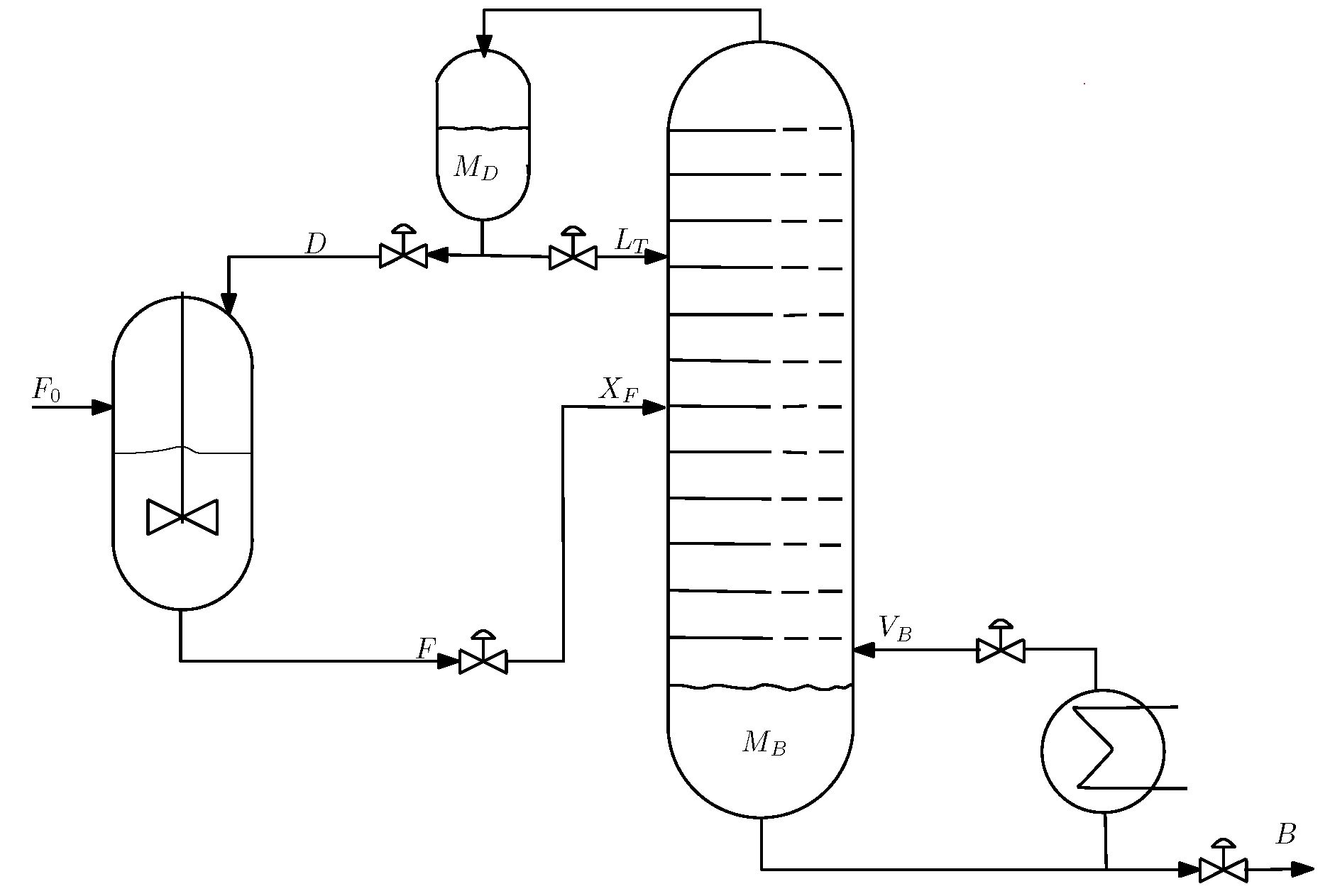
4. Numerical Case Study

4.1. Process Description

We demonstrate the path-following NMPC (pf-NMPC) on an isothermal reactor and separator process depicted in Figure 2. The continuously-stirred tank reactor (CSTR) is fed with a stream $F_0$ containing 100% component $\mathcal{A}$ and a recycler R from the distillation column. A first-order reaction $\mathcal{A}\to \mathcal{B}$ takes place in the CSTR where $\mathcal{B}$ is the desired product and the product with flow rate F is fed to the column. In the distillation column, the unreacted raw material is separated from the product and recycled into the reactor. The desired product $\mathcal{B}$ leaves the distillation column as the bottom product, which is required to have a certain purity. Reaction kinetic parameters for the reactor are described in

Table 1. Reaction kinetics parameters.

Reaction	Reaction Rate Constant (min−1)	Activation Energy (in J/mol)
$\mathcal{A}\to \mathcal{B}$	$1\times {10}^8$	$6\times {10}^4$

. The distillation column model is taken from [29].

Table 2. Distillation Column A parameters.

Parameter	Value
${\alpha }_{AB}$	1.5
number of stages	41
feed stage location	21

summarizes the parameters used in the distillation. In total, the model has 84 state variables of which 82 are from the distillation (concentration and holdup for each stage) and two from the CSTR (one concentration and one holdup).

The stage cost of the economic objective function to optimize under operation is:

$$J=p_F{F}_0+p_V{V}_B-p_{B}B,$$

(20)

where $p_F$ is the feed cost, $p_V$ is the steam cost and $p_B$ is the product price. The price setting is $p_F=1\$/kmol$, $p_V=0.02\$/kmol$, $p_B=2\$/kmol$. The operational constraints are the concentration of the bottom product ($x_B\le 0.1$), as well as the liquid holdup at the bottom and top of the distillation column and in the CSTR ($0.3\le M_{\left\{B,D,CSTR\right\}}\le 0.7$ kmol). The control inputs are reflux flow ($L_T$), boil-up flow ($V_B$), feeding rate to the distillation (F), distillate (top) and bottom product flow rates (D and B). These control inputs have bound constraints as follows:

$$\left[\begin{array}{c}0.1\\ 0.1\\ 0.1\\ 0.1\\ 0.1\end{array}\right]\le \left[\begin{array}{c}{L}_T\\ V_B\\ F\\ D\\ B\end{array}\right]\le \left[\begin{array}{c}10\\ 4.008\\ 10\\ 1.0\\ 1.0\end{array}\right]\left(\mathrm{kmol}/\min \right).$$

First, we run a steady-state optimization with the following feed rate $F_0=0.3$ (kmol/min). This gives us the optimal values for control inputs and state variables. The optimal steady state input values are ${\mathbf{u}}_s={\left[\begin{array}{ccccc}1.18& 1.92& 1.03& 0.74& 0.29\end{array}\right]}^T.$ The optimal state and control inputs are used to construct regularization term added to the objective function (20). Now, the regularized stage becomes:

$$J_m=p_F{F}_0+p_V{V}_B-p_{B}B-p_{D}D+{\left(\mathbf{z}-{\mathbf{x}}_s\right)}^T{\mathbf{Q}}_1\left(\mathbf{z}-{\mathbf{x}}_s\right)+{\left(\mathbf{v}-{\mathbf{u}}_s\right)}^T{\mathbf{Q}}_2\left(\mathbf{v}-{\mathbf{u}}_s\right).$$

(21)

The weights ${\mathbf{Q}}_1$ and ${\mathbf{Q}}_2$ are selected to make the rotated stage cost of the steady state problem strongly convex; for details, see [24]. This is done to obtain an economic NMPC controller that is stable.

Secondly, we set up the NLP for calculating the predicted state variables $\mathbf{z}$ and predicted control inputs $\mathbf{v}$. We employ a direct collocation approach on finite elements using Lagrange collocation to discretize the dynamics, where we use three collocation points in each finite element. By using the direct collocation approach, the state variables and control inputs become optimization variables.

The economic NMPC case study is initialized with the steady state values for a production rate $F_0=0.29$ kmol/min, such that the economic NMPC controller is effectively controlling a throughput change from $F_0=0.29$ kmol/min to $F_0=0.3$ kmol/min. We simulate 150 MPC iterations, with a sample time of 1 min. The prediction horizon of the NMPC controller is set to 30 min. This setting results in an NLP with 10,314 optimization variables. We use CasADi [30] (Version 3.1.0-rc1) with IPOPT [31] as the NLP solver. For the QPs, we use MINOS QP [32] from TOMLAB.

4.2. Comparison of the Open-Loop Optimization Results

In this section, we compare the solutions obtained from the path-following algorithm with the “true” solution of the optimization problem ${\mathcal{P}}_{nmpc}$ obtained by solving the full NLP. To do this, we consider the second MPC iteration, where the path-following asNMPC is used for the first time to correct the one-sample ahead-prediction (in the first MPC iteration, to start up the asNMPC procedure, the full NLP is solved twice). We focus on the interesting case where the predicted state is corrupted by noise, such that the path-following algorithm is required to update the solution. In Figure 3, we have plotted the difference between a selection of predicted states, obtained by applying the path-following NMPC approaches, and the ideal NMPC approach.

We observe that the one-step pure-predictor tracks the ideal NMPC solution worst and the four-step path-following with predictor-corrector tracks best. This happens because the predictor-corrector path-following QP has an additional linear term in the objective function and constraint for the purpose of moving closer to the solution of the NLP (the “corrector” component), as well as tracing the first-order estimate of the change in the solution (the “predictor”). The four-step path-following performs better because a smaller step size gives finer approximation of the parametric NLP solution.

This is also reflected in the average approximation errors given in

Table 3. Approximation error using path-following algorithms. asNMPC, advanced-step NMPC (asNMPC); QP, quadratic programming.

Average Approximation Error between ideal NMPC and Path-Following (PF) asNMPC
PF with predictor QP, 1 step PF with predictor QP, 4 steps PF with predictor-corrector QP, 1 step PF with predictor-corrector QP, 4 steps	4.516 4.517 1.333 × 10−2 1.282 × 10−2

. The average approximation error has been calculated by averaging the error one-norm ${\left|\left|{\chi }_{path-following}-{\chi }_{idealNMPC}\right|\right|}_1$ over all MPC iterations.

We observe that in this case study, the accuracy of a single predictor-corrector step is almost as good as performing four predictor-corrector steps along the path. That is, a single predictor-corrector QP update may be sufficient for this application. However, in general, in the presence of larger noise magnitudes and longer sampling intervals, which cause poorer predictions, a single-step update may no longer lead to good approximations. We note the large error in the pure-predictor path-following method for the solution accuracy of several orders of magnitude.

On the other hand, given that the optimization vector χ has dimension 10,164 for our case study, the average one-norm approximation error of ca. 4.5 does result in very small errors on the individual variables.

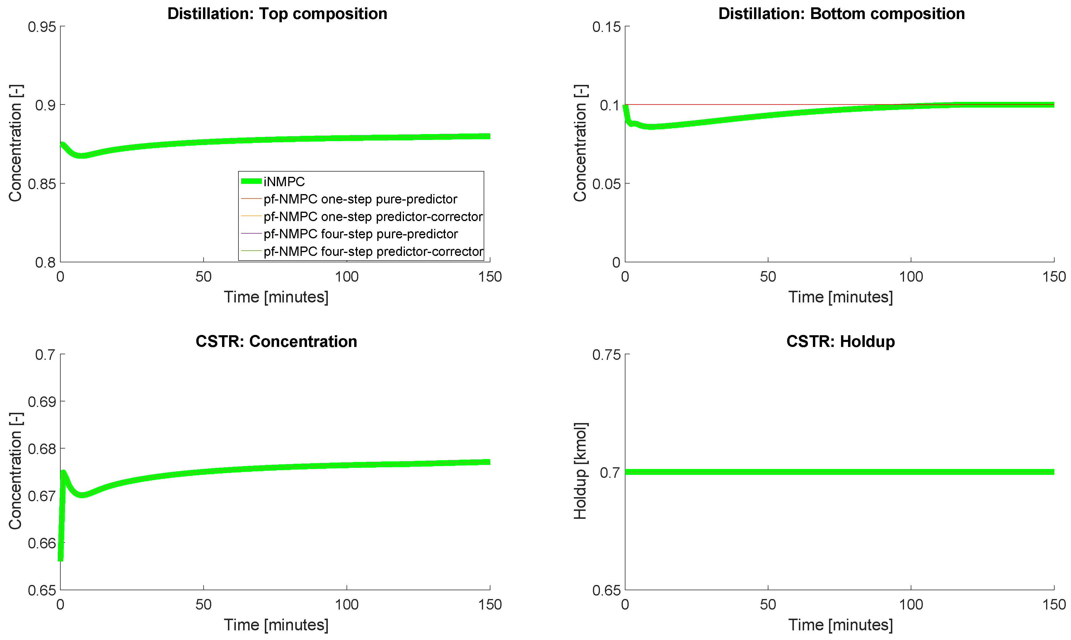
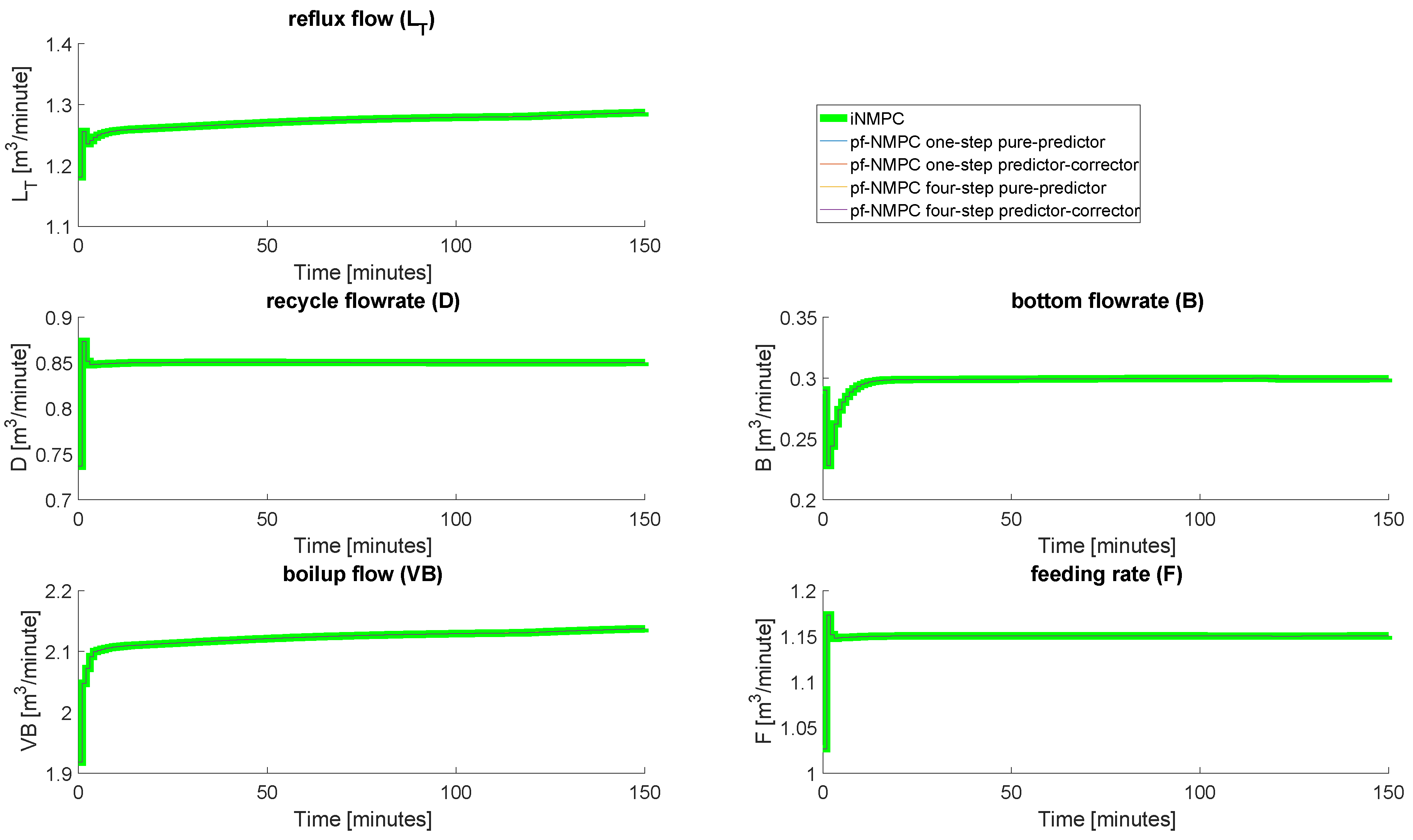
4.3. Closed-Loop Results: No Measurement Noise

In this section, we compare the results for closed loop process operation. We consider first the case without measurement noise, and we compare the results for ideal NMPC with the results obtained by the path-following algorithm with the pure-predictor QP (10) and the predictor-corrector QP (12). Figure 4 shows the trajectories of the top and bottom composition in the distillation column and the reactor concentration and holdup. Note that around 120 min, the bottom composition constraint in the distillation column becomes active, while the CSTR holdup is kept at its upper bound all of the time (any reduction in the holdup will result in economic and product loss).

In this case (without noise), the prediction and the true solution only differ due to numerical noise. There is no need to update the prediction, and all approaches give exactly the same closed-loop behavior. This is also reflected in the accumulated stage cost, which is shown in

Table 4. Comparison of economic NMPC controllers (no noise). Accumulated stage cost in $.

Economic NMPC Controller		Accumulated Stage Cost
iNMPC		−296.42
pure-predictor QP:
	pf-NMPC one step	−296.42
	pf-NMPC four steps	−296.42
predictor-corrector QP:
	pf-NMPC one step	−296.42
	pf-NMPC four steps	−296.42

.

The closed-loop control inputs are given in Figure 5. Note here that the feed rate into the distillation column is adjusted such that the reactor holdup is at its constraint all of the time.

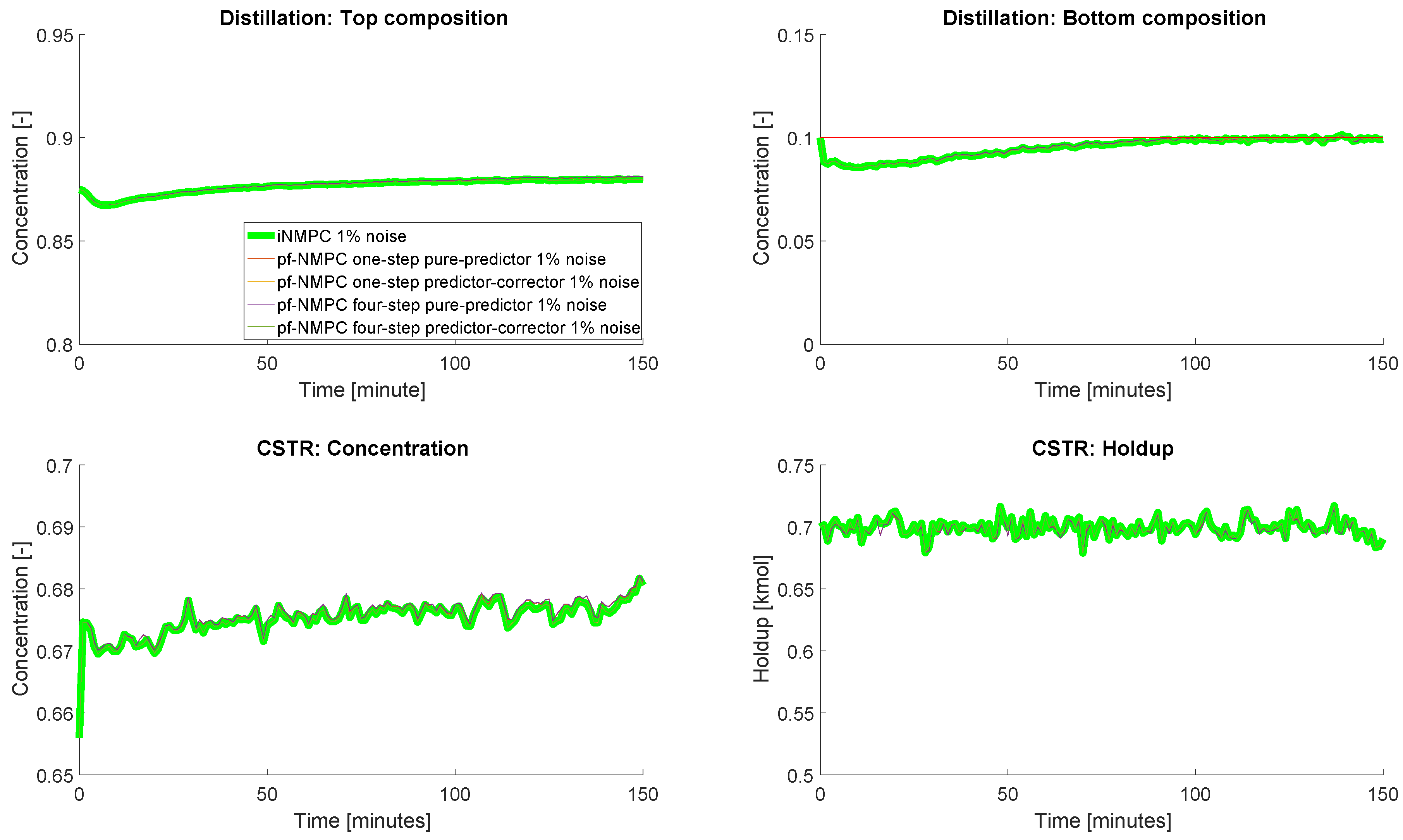
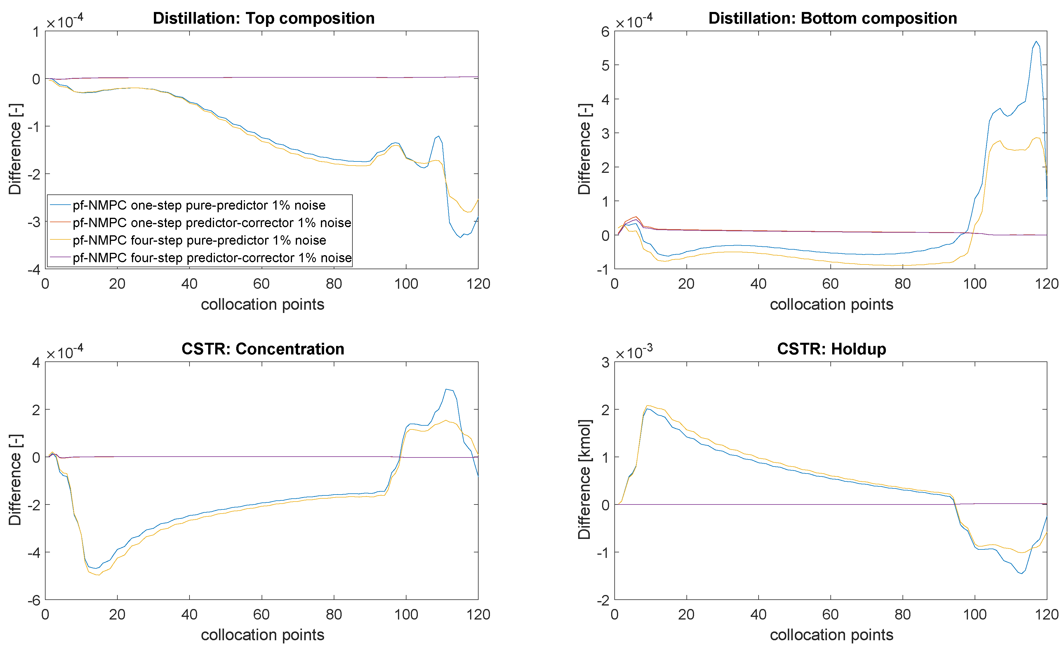
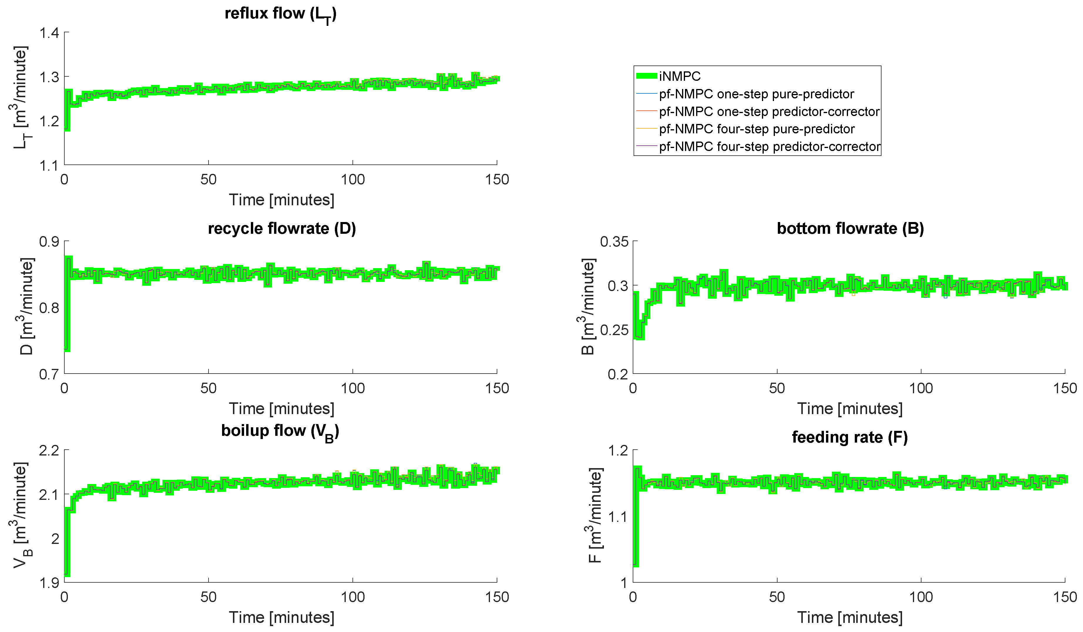
4.4. Closed-Loop Results: With Measurement Noise

Next, we run simulations with measurement noise on all of the holdups in the system. The noise is taken to have a normal distribution with zero mean and a variance of one percent of the steady state values. This will result in corrupted predictions that have to be corrected for by the path-following algorithms. Again, we perform simulations with one and four steps of pure-predictor and predictor-corrector QPs.

Figure 6 shows the top and bottom compositions of the distillation column, together with the concentration and holdup in the CSTR. The states are obtained under closed-loop operation with the ideal and path-following NMPC algorithms. Due to noise, it is not possible to avoid the violation of the active constraints in the holdup of the CSTR and the bottom composition in the distillation column. This is the case for both the ideal NMPC and the path-following approaches.

The input variables shown in Figure 7 are also reflecting the measurement noise, and again, we see that the fast sensitivity NMPC approaches are very close to the ideal NMPC inputs.

Finally, we compare the accumulated economic stage cost in

Table 5. Comparison of economic NMPC controllers (with noise). Accumulated stage cost in $.

Economic NMPC Controller		Accumulated Stage Cost
iNMPC		−296.82
pure-predictor QP:
	pf-NMPC one step	−297.54
	pf-NMPC four steps	−297.62
predictor-corrector QP:
	pf-NMPC one step	−296.82
	pf-NMPC four steps	−296.82

.

Here, we observe that our proposed predictor-corrector path-following algorithm performs identically to the ideal NMPC. This is as expected, since the predictor-corrector path-following algorithm is trying to reproduce the true NLP solution. Interestingly, in this case, the larger error in the pure predictor path-following NMPC leads to a better economic performance of the closed loop system. This behavior is due to the fact that the random measurement noise can have a positive and a negative effect on the operation, which is not taken into account by the ideal NMPC (and also the predictor-corrector NMPC). In this case, the inaccuracy of the pure-predictor path-following NMPC led to better economic performance in the closed loop. However, it could also have been the opposite.

5. Discussion and Conclusions

We applied the path-following ideas developed in Jäschke et al. [24] and Kungurtsev and Diehl [28] to a large-scale process containing a reactor, a distillation column and a recycle stream. Compared with single-step updates based on solving a linear system of equations as proposed by [10], our path-following approach requires somewhat more computational effort. However, the advantage of the path-following approach is that active set changes are handled rigorously. Moreover, solving a sequence of a few QPs can be expected to be much faster than solving the full NLP, especially since they can be initialized very well, such that the computational delay between obtaining the new state and injecting the updated input into the plant is still sufficiently small. In our computations, we have considered a fixed step-size for the path-following, such that the number of QPs to be solved is known in advance.

The case without noise does not require the path-following algorithm to correct the solution, because the prediction and the true measurement are identical, except for numerical noise. However, when measurement noise is added to the holdups, the situation becomes different. In this case, the prediction and the measurements differ, such that an update is required. All four approaches track the ideal NMPC solution to some degree; however, in terms of accuracy, the predictor-corrector performs consistently better. Given that the pure sensitivity QP and the predictor-corrector QP are very similar in structure, it is recommended to use the latter in the path-following algorithm, especially for highly nonlinear processes and cases with significant measurement noise.

We have presented basic algorithms for path-following, and they seem to work well for the cases we have studied, such that the path-following algorithms do not diverge from the true solution. In principle, however, the path-following algorithms may get lost, and more sophisticated implementations need to include checks and safeguards. We note, however, that the application of the path-following algorithm in the advanced-step NMPC framework has the desirable property that the solution of the full NLP acts as a corrector, such that if the path-following algorithm diverges from the true solution, this will be most likely for only one sample time, until the next full NLP is solved.

The path-following algorithm in this paper (and the corresponding QPs) still relies on the assumption of linearly-independent constraint gradients. If there are path-constraints present in the discretized NLP, care must be taken to formulate them in such a way that LICQ is not violated. In future work, we will consider extending the path-following NMPC approaches to handle more general situations with linearly-dependent inequality constraints.

References

1. Zanin, A.C.; Tvrzská de Gouvêa, M.; Odloak, D. Industrial implementation of a real-time optimization strategy for maximizing production of LPG in a FCC unit. Comput. Chem. Eng. 2000, 24, 525–531. [Google Scholar] [CrossRef]
2. Zanin, A.C.; Tvrzská de Gouvêa, M.; Odloak, D. Integrating real-time optimization into the model predictive controller of the FCC system. Control Eng. Pract. 2002, 10, 819–831. [Google Scholar] [CrossRef]
3. Rawlings, J.B.; Amrit, R. Optimizing process economic performance using model predictive control. In Nonlinear Model Predictive Control; Springer: Berlin/Heidelberg, Germany, 2009; Volume 384, pp. 119–138. [Google Scholar]
4. Rawlings, J.B.; Angeli, D.; Bates, C.N. Fundamentals of economic model predictive control. In Proceedings of the 51st IEEE Conference on Conference on Decision and Control (CDC), Maui, HI, USA, 10–13 December 2012.
5. Ellis, M.; Durand, H.; Christofides, P.D. A tutorial review of economic model predictive methods. J. Process Control 2014, 24, 1156–1178. [Google Scholar] [CrossRef]
6. Tran, T.; Ling, K.-V.; Maciejowski, J.M. Economic model predictive control—A review. In Proceedings of the 31st ISARC, Sydney, Australia, 9–11 July 2014.
7. Angeli, D.; Amrit, R.; Rawlings, J.B. On average performance and stability of economic model predictive control. IEEE Trans. Autom. Control 2012, 57, 1615–1626. [Google Scholar] [CrossRef]
8. Idris, E.A.N.; Engell, S. Economics-based NMPC strategies for the operation and control of a continuous catalytic distillation process. J. Process Control 2012, 22, 1832–1843. [Google Scholar] [CrossRef]
9. Findeisen, R.; Allgöwer, F. Computational delay in nonlinear model predictive control. In Proceedings of the International Symposium on Advanced Control of Chemical Proceses (ADCHEM’03), Hongkong, China, 11–14 January 2004.
10. Zavala, V.M.; Biegler, L.T. The advanced-step NMPC controller: Optimality, stability, and robustness. Automatica 2009, 45, 86–93. [Google Scholar] [CrossRef]
11. Diehl, M.; Bock, H.G.; Schlöder, J.P. A real-time iteration scheme for nonlinear optimization in optimal feedback control. SIAM J. Control Optim. 2005, 43, 1714–1736. [Google Scholar] [CrossRef]
12. Würth, L.; Hannemann, R.; Marquardt, W. Neighboring-extremal updates for nonlinear model-predictive control and dynamic real-time optimization. J. Process Control 2009, 19, 1277–1288. [Google Scholar] [CrossRef]
13. Biegler, L.T.; Yang, X.; Fischer, G.A.G. Advances in sensitivity-based nonlinear model predictive control and dynamic real-time optimization. J. Process Control 2015, 30, 104–116. [Google Scholar] [CrossRef]
14. Wolf, I.J.; Marquadt, W. Fast NMPC schemes for regulatory and economic NMPC—A review. J. Process Control 2016, 44, 162–183. [Google Scholar] [CrossRef]
15. Diehl, M.; Bock, H.G.; Schlöder, J.P.; Findeisen, R.; Nagy, Z.; Allgöwer, F. Real-time optimization and nonlinear model predictive control of processes governed by differential-algebraic equations. J. Process Control 2002, 12, 577–585. [Google Scholar] [CrossRef]
16. Gros, S.; Quirynen, R.; Diehl, M. An improved real-time economic NMPC scheme for Wind Turbine control using spline-interpolated aerodynamic coefficients. In Proceedings of the 53rd IEEE Conference on Decision and Control, Los Angeles, CA, USA, 15–17 December 2014; pp. 935–940.
17. Gros, S.; Vukov, M.; Diehl, M. A real-time MHE and NMPC scheme for wind turbine control. In Proceedings of the 52nd IEEE Conference on Decision and Control, Firenze, Italy, 10–13 December 2013; pp. 1007–1012.
18. Ohtsuka, T. A continuation/GMRES method for fast computation of nonlinear receding horizon control. Automatica 2004, 40, 563–574. [Google Scholar] [CrossRef]
19. Li, W.C.; Biegler, L.T. Multistep, Newton-type control strategies for constrained nonlinear processes. Chem. Eng. Res. Des. 1989, 67, 562–577. [Google Scholar]
20. Pirnay, H.; López-Negrete, R.; Biegler, L.T. Optimal sensitivity based on IPOPT. Math. Program. Comput. 2002, 4, 307–331. [Google Scholar] [CrossRef]
21. Yang, X.; Biegler, L.T. Advanced-multi-step nonlinear model predictive control. J. Process Control 2013, 23, 1116–1128. [Google Scholar] [CrossRef]
22. Kadam, J.; Marquardt, W. Sensitivity-based solution updates in closed-loop dynamic optimization. In Proceedings of the DYCOPS 7 Conference, Cambridge, MA, USA, 5–7 July 2004.
23. Würth, L.; Hannemann, R.; Marquardt, W. A two-layer architecture for economically optimal process control and operation. J. Process Control 2011, 21, 311–321. [Google Scholar] [CrossRef]
24. Jäschke, J.; Yang, X.; Biegler, L.T. Fast economic model predictive control based on NLP-sensitivities. J. Process Control 2014, 24, 1260–1272. [Google Scholar] [CrossRef]
25. Fiacco, A.V. Introduction to Sensitivity and Stability Analysis in Nonlinear Programming; Academic Press: New York, NY, USA, 1983. [Google Scholar]
26. Bonnans, J.F.; Shapiro, A. Optimization problems with perturbations: A guided tour. SIAM Rev. 1998, 40, 228–264. [Google Scholar] [CrossRef]
27. Levy, A.B. Solution sensitivity from general principles. SIAM J. Control Optim. 2001, 40, 1–38. [Google Scholar] [CrossRef]
28. Kungurtsev, V.; Diehl, M. Sequential quadratic programming methods for parametric nonlinear optimization. Comput. Optim. Appl. 2014, 59, 475–509. [Google Scholar] [CrossRef]
29. Skogestad, S.; Postlethwaite, I. Multivariate Feedback Control: Analysis and Design; Wiley-Interscience: Hoboken, NJ, USA, 2005. [Google Scholar]
30. Andersson, J. A General Purpose Software Framework for Dynamic Optimization. Ph.D. Thesis, Arenberg Doctoral School, KU Leuven, Leuven, Belgium, October 2013. [Google Scholar]
31. Wächter, A.; Biegler, L.T. On the implementation of an interior-point filter line-search algorithm for large-scale nonlinear programming. Math. Program. 2006, 106, 25–57. [Google Scholar] [CrossRef]
32. Murtagh, B.A.; Saunders, M.A. A projected lagrangian algorithm and its implementation for sparse nonlinear constraints. Math. Program. Study 1982, 16, 84–117. [Google Scholar]
Figure 1. (a) Constraints of NLP (16) in Example 1 and (b) their linearization at x ^ = ( 1 , 2 ) and t = 0.
Processes 05 00008 g001
Figure 2. Diagram of continuously-stirred tank reactor (CSTR) and distillation column.
Processes 05 00008 g002
Figure 3. The difference in predicted state variables between ideal NMPC (iNMPC) and path-following NMPC (pf-NMPC) from the second iteration.
Processes 05 00008 g003
Figure 4. Recycle composition, bottom composition, reactor concentration and reactor holdup.
Processes 05 00008 g004
Figure 5. Optimized control inputs.
Processes 05 00008 g005
Figure 6. Recycle composition, bottom composition, reactor concentration and reactor holdup.
Processes 05 00008 g006
Figure 7. Optimized control inputs.
Processes 05 00008 g007