
Performance Evaluation of Real Industrial RTO Systems


1
Chemical Engineering Program, COPPE, Federal University of Rio de Janeiro, Cidade Universitária, Rio de Janeiro, RJ 21945-970, Brazil
2
Petrobras—Petróleo Brasileiro SA, Corporate University, Rio de Janeiro, RJ 20211-230, Brazil
*
Author to whom correspondence should be addressed.
Processes 2016, 4(4), 44; https://doi.org/10.3390/pr4040044
Submission received: 4 October 2016
/
Revised: 5 November 2016
/
Accepted: 14 November 2016
/
Published: 22 November 2016
(This article belongs to the Special Issue Real-Time Optimization)
Abstract
:The proper design of RTO systems’ structure and critical diagnosis tools is neglected in commercial RTO software and poorly discussed in the literature. In a previous article, Quelhas et al. (Can J Chem Eng., 2013, 91, 652–668) have reviewed the concepts behind the two-step RTO approach and discussed the vulnerabilities of intuitive, experience-based RTO design choices. This work evaluates and analyzes the performance of industrial RTO implementations in the face of real settings regarding the choice of steady-state detection methods and parameters, the choice of adjustable model parameters and selected variables in the model adaptation problem, the convergence determination of optimization techniques, among other aspects, in the presence of real noisy data. Results clearly show the importance of a robust and careful consideration of all aspects of a two-step RTO structure, as well as of the performance evaluation, in order to have a real and undoubted improvement of process operation.
1. Introduction
Real-time optimization systems (RTO) are a combined set of techniques and algorithms that continuously evaluate process operating conditions and implement business-focused decisions in order to improve process performance in an autonomous way. It relies on static real-time optimization strategies [1,2,3,4,5], which have been designated in the literature by real-time optimization [6], on-line optimization [7,8] and optimizing control [9], for translating a product recipe from the scheduling layer into the best set of reference values to the model predictive control (MPC) layer [10]. The two-step approach, a model-based technique, is the most common (and possibly the only) static real-time optimization strategy available in commercial RTO systems [11,12,13]. Its name derives from the procedure employed for determining the set of decision variables, where plant information is used to update model parameters based on the best fitting of measurements in the first step, and afterwards, the updated model is used to calculate the set of decision variable values that are assumed to lead the process to its best economic performance. RTO systems are widely used in the petrochemical industry as a part of modern day control systems [14,15,16,17], but may also be found in other sectors, such as the pulp and paper industry [18].
Great advantages are attributed to the use of a priori information in the form of a process model, and model-based techniques may present superior performance among others; generally, the more accurate the model, the better will be the RTO system performance [19,20]. Thus, such RTO applications are typically based on rigorous steady-state models of processes. However, it has long been shown that manipulation of model parameters to fit available process measurements does not necessarily guarantee the construction of an adequate model for process optimization [21,22]. For this reason, known as plant-model mismatch, some alternative procedures have been proposed (e.g., [23,24,25,26]) based on stronger mathematical requirements and constraints that guarantee the optimality of process operation. Unfortunately, these procedures demand a series of time-consuming experimental measurements in order to evaluate the gradients of a large set of functions and variables. Given the considerable impact on productivity, these implementations are virtually absent in current industrial practice. Nevertheless, commercial software is usually based on a very standard two-step structure and does not even take into account collateral improvements of this approach, such as the use of multiple datasets [27], input excitation design [28,29] or automated diagnosis [30].
In fact, plant-model mismatch is not the only vulnerability of RTO systems, whose performance can also be jeopardized by incomplete and corrupted process information, absence of knowledge regarding measurement errors and performance issues related to numerical optimization techniques [31]. In addition, the use of continuous system diagnostic tools is not common, neither in the literature, nor in commercial RTO systems. In this context, there are few works in the literature dedicated to diagnosing and criticizing the obtained results and software tools of real-time optimization. Although it is possible to find some valuable criticism about RTO implementations [32,33], the discussion is normally presented in general terms, making it hard for practitioners to distinguish process-related features from methodological limitations of the RTO approach.
The present work aims at presenting the performance evaluation of real industrial RTO systems. The characteristics of operation shared by two RTO commercial packages from two different world-class providers will be presented, which are actual implementations of the two-step RTO approach, currently in use on crude oil distillation units from two commercial-scale Brazilian petroleum refineries. The aim is not at exhausting the many aspects involved, but rather presenting some features of large-scale RTO systems that are commonly blurred due to the great amount of information required by optimization systems.
This article presents the basics of a two-step-based RTO system in Section 2. Then, it briefly presents a general description of an industrial RTO system in Section 3, along with major details about the two commercial systems discussed in this paper. The results of industrial RTO implementations are discussed in Section 4. Finally, Section 5 suggests some concluding remarks.
2. Problem Statement
The idea of optimization is to find the set of values for decision variables that renders the extreme of a function, while satisfying existing constraints. In this context, the main task of an optimization system is to tune the vector of available degrees of freedom of a process in order to reach the “best” value of some performance metric.
The vector of decision variables, , is a subset of a larger set of input variables, , that is supposed to determine how the process behaves, as reflected by the set of output variables, , thus establishing a mapping of . If a set of indexes is used to define the vector of decision variables, thus:
where refers to the length of the n-th-dimension of an array. Common criteria used to select are the easiness of variable manipulation in the plant, the requirements of the industry and the effects of the decision variables on process performance [34]. Characteristics of the feed, such as flow rate and temperature, are commonly assigned as decision variables.
Besides the identification of indexes for decision variables from the set of inputs, we could identify a group that represents the expectation of some elements of (e.g., vessel temperature, feed composition, heat transfer coefficients, decision variables, among others) to change along an operational scenario, being defined by a set of indexes . In turn, those elements supposed to remain constant (e.g., tube diameters, coolant temperature, catalyst surface area, system equilibrium states, thermodynamic constants, etc.) are represented by the set of indexes . Mathematically, this can be stated as:
Another important subset of input variables is external disturbances. As the system evolves with time and disturbances of a stochastic nature are present, it is convenient to establish a partition dividing disturbances into stationary and nonstationary, defining a two-time scale. When doing this, we assume that nonstationary disturbance components are “quickly” varying, and there is a regulatory control in charge of suppressing their influence, in such a way that they are irrelevant for the long-term optimization of the process [35]. Thus, there remains only the persistent and/or periodic disturbances, which have to be included in the long-term optimization. Employing a pseudo-steady-state assumption, plant dynamics may be neglected, and process evolution can be represented as a sequence of successive steady-state points. Hereafter, an element in this sequence is represented either as an array or with the help of a subscript k. Accordingly, we can state the following for the elements of supposed to remain constant:
The process behavior, as described by and , will thus present a performance metric . The performance metric is the result of the mapping , where ϕ vary with the underlying process and may be defined in several ways. Nevertheless, it is conveniently represented by an economic index, such as profit, in most cases. Roughly, profit is determined as the product value minus the costs of production, such as raw material and utility costs. For example, in the work of Bailey et al. [36] applied to the optimization of a hydrocracker fractionation plant, profit was adopted as the performance metric, represented by the sum of the value of feed and product streams (valued as gasoline), the value of feed and product streams (priced as fuel), the value of pure component feeds and products and the cost of utilities. As stated above, optimization is the act of selecting the set of values for vector that conducts the process to the most favorable , i.e., selecting a proper , such that given and at steady-state point k.
Input and output variables are related through a set of equations that express conservation balances (mass, energy, momentum), equipment design constraints, etc., expressed as a set f of equations called the process model. Another set of relationships describes safety conditions, product specifications and other important requirements, so that f and represent the process optimization constraints. Given the performance metric and the process optimization constraints, the static process optimization is written as the following nonlinear programming problem:
Process information is primarily obtained through sensors and analyzers, which translate physical and chemical properties of streams and equipment into more useful process values. The information carried by the process is represented by the whole set of process variables . Unfortunately, in any real industrial case, the full vector is not available, and the lack of information is related mainly to the absence of measurements due to management decisions made during the process design. These decisions are based on sensor costs and known limitations of sensor technology, as well as the lack of knowledge about the variables that constitute the real vector . As a consequence, the real system is known only through the elements of , i.e.:
If, at steady instant k, the real plant is under the influence of , the problem posed to the RTO system may be described in the following terms: starting from the available information set , the RTO has to find out that drives the process to . In a scenario of limited knowledge of the system, reflected by incomplete information of the current state , a new expanded set of information, , has to be produced from , so that the optimization procedure is able to identify the right set . We assume that, in the face of the structure of the process optimization constraints (f and ), the set of fresh measurements, , carries an excess of information that can be used to update some elements of the vector of offsets, Θ, which are modifiers of , so that .
Due to restrictions regarding the available information, in most problems only a subset , represented by the index , can accommodate the existing excess of information present in measurements. The remaining set of offsets, represented by the index , is supposed to be kept at (assumed) base values, as shown in the following:
It must be emphasized that this formulation implicitly assumes that the only process variables actually changing during real-world operation are the sets of measured variables and updated parameters, in such a way that it is possible to accommodate all uncertainties in the updated parameters. In other words, it is assumed that there is no plant-model mismatch.
Information provided by sensors is expected to be similar, but not equal to the “true” information produced by the process. Sensors incorporate into the process signal some features that are not related to the behavior of variables, so that the observed values of measured variables are different from “true” values . To cope with this kind of uncertainty, the measurement error is usually modeled as the result of two components, a deterministic (the “truth”) and a stochastic one (the “noise”). Defining , a convenient form of modeling measurement errors consists in the following additive relation:
where represents the values of acquired with the help of process instrumentation, are values of estimated by the process model f, which is a function of θ, and ε is the measurement error vector, being a random variable.
In an ideal scenario, the RTO implementation relies on perfect knowledge of the input set , of the process optimization constraints f and and of the performance metric ϕ. In the context of the two-step RTO scheme, the adaptation step performs the task of selecting the set that better explains measurements in light of the plant model. In order to do that, besides the model structure, it is also necessary to take into account the probability of the occurrence of noise. In other words, it is necessary to find the set that most likely gives rise to the real corrupted measurements . This estimation problem is successfully dealt with by the statistical approach of maximum likelihood estimation [37], as described in Equation (9), which consists of maximizing the likelihood function under constraints imposed by the process model. It should be noted that the elements of included in the objective function are those related to the indexes , where , according to decisions made during the design of the RTO structure.
If ε follows a Gaussian probability density function, such that , , and , the problem defined in Equation (9) becomes the weighted least squares (WLS) estimation:
where is the covariance matrix of , which is normally assumed to be diagonal (i.e., measurement fluctuations are assumed to be independent).
In summary, a typical RTO system based on the two-step approach will, at any time: (i) gather information from the plant; (ii) detect stationarity in data series, defining a new steady state k; (iii) solve the model updating problem (such as Equation (10)); and (iv) determine the best set of decision variables by solving Equation (5).
3. RTO System Description
The traditional implementation of an RTO system is based on the two-step approach, which corresponds to both commercial systems considered in this work. A typical structure of a commercial RTO system is shown in Figure 1, which relates to an application in a crude oil atmospheric distillation unit. This RTO system has the following main modules:
- (a)
- Steady-state detection (SSD), which states if the plant is at steady state based on the data gathered from the plant within a time interval;
- (b)
- Monitoring sequence (MON), which is a switching method for executing the RTO iteration based on the information of the unit’s stability, the unit’s load and the RTO system’s status; the switching method triggers the beginning of a new cycle of optimization and commonly depends on a minimal interval between successive RTO iterations, which typically corresponds to 30 min to 2 h for distillation units;
- (c)
- Execution of the optimization layer based on the two-step approach, thus adapting the stationary process model and using it as a constraint for solving a nonlinear programming problem representing an economic index.
The RTO is integrated with the following layers:
- production planning and scheduling, which transfer information to it;
- storage logistics, which has information about the composition of feed tanks;
- Distributed control system (DCS) and database, which deliver measured values.
In the present work, the discussed results are associated with two RTO systems actually running in crude oil distillation units in distinct commercial-scale refineries located in Brazil. Both RTO commercial packages are from two different world-class providers. In doing this, we aim at preferably using one for analyzing the generated data (referred to as Tool A), while the other is used to compare the systems’ architecture and algorithms (referred to as Tool B). The set of data from RTO system Tool A includes the results obtained from 1000 RTO iterations, which corresponds to a three-month period. In addition, Tool A has a static process model comprised by approximately equations.
4. Industrial RTO Evaluation
The evaluation of real RTO implementations is presented in this section focusing on two aspects: steady-state detection and adaptation and optimization. The former is supported by the fact that the applied process model is static, and only stationary data will render a valid process adaptation. Acting as a gatekeeper in the system, steady-state detection has a great influence on RTO performance. However, it is hardly discussed in the RTO literature. On the other hand, the latter is extensively studied in many articles. Analyses here will be mainly based on problem formulation issues and observed variability in the results.
4.1. Steady-State Detection
An important element of RTO systems refers to the mechanism that triggers the process optimization. Traditionally, it is based on the stationarity of measured process data and is accomplished by the SSD module.
4.1.1. Tool A
Tool A offers two options for detecting the steady state, shown to the user under the terms “statistical method” and “heuristic method”. Formally, the former corresponds to the statistical test suggested by von Neumann [38]. This test establishes the comparison of the total variance of a signal and the variance of the difference between two successive points within this signal. The total variance of a signal x for a data window with n points is given by the sample variance (), according to:
where is the sample mean, while the variance of the difference between two successive points is expressed by:
These two variances give rise to the statistic R [38,39], which is eventually expressed as C [40], defined as:
Nevertheless, Tool A adopts this method with a slight difference. There is an extra option, where the user may define a tuning parameter, , which changes the definition of R in the following way:
Then, the signal is static if R is greater than a critical value (or if C is lower than a critical value ).
The so called “heuristic method” makes use of two versions of the original signal subjected to filters with distinct cut frequencies, which are indirectly manipulated by the user when defining the parameters and , according to Equation (15). The filtering (or simplification) represents an exponentially-weighted moving average, or conventional first-order filter, that requires little storage and is computationally fast [41]. The signal version with a low cut frequency () is called the “heavy filter”, while the other () is called the “light filter”. The test is very simple and establishes that the signal is stationary if the difference between these two filtered signals is lower than a predetermined tolerance.
It is worth noting that both the “statistical method” and the “heuristic method” are somewhat combined in the method proposed by Cao and Rhinehart [41]. The method is based on the R-statistic, using a ratio of two variances measured on the same set of data by two methods and employs three first-order filter operations, providing computational efficiency and robustness to process noise and non-noise patterns. Critical values and statistical evidence of the method to reject the steady-state hypothesis, as well as to reject the transient state hypothesis have already been discussed in the literature [42,43]. This method was also modified in [44] by optimizing the filter constants so as to minimize Type I and II errors and simultaneously reduce the delay in state detection.
From a user point of view, the experience shows that the “heuristic method” is overlooked with respect to the “statistical method”. This might be related to the greater dependence of this method on user inputs, where there must be a total of parameters, since each signal requires a value of , and tolerance. Besides, the tolerances are not normalized and must be provided in accordance with the unit of the original signal.
Considering the use of RTO package Tool A, each parameter in these methods is defined by the user. In the statistical method (SM), the presence of the tolerance (Equation (14)) allows, in practice, the user to define what is (or will be) considered stationary. Thus, any statistical foundation claimed by the method is jeopardized by a user-defined choice based on its own definition. In the case of the heuristic method (HM), the arbitrary nature of the parameters puts the user in charge of the decision making process, directing stationarity towards its own beliefs, as it is for SM. In spite of this, given the large number of inputs, it is likely that the user will not be able to anticipate the effects of its choice on the signal shape.
4.1.2. Tool B
Tool B also presents two options for stating signals’ stationarity. One of them is the R-statistic (Equation (13)), as described above for Tool A. The other option is comprised by a hypothesis test to assess whether or not the average values of two halves of a time window are identical. First, a hypothesis test is applied to the ratio between the variances. This is accomplished by means of the F-statistic [45], where the two subsequent time intervals i and j have data points. If the null hypothesis of identical variances is rejected, then the mean values and are compared by means of the variable [46,47], defined as:
If the values within time intervals i and j are normal and independent, will follow the Student t-distribution with degrees of freedom, determined by:
In turn, if the null hypothesis of identical variances is accepted, a second test assesses if the difference between these averages is lower than a given tolerance (ϵ). This is supported by the assumption that the t-statistic determined by Equations (18) and (19) follows a Student t with degrees of freedom. In the particular case of Tool B, these tests always have a fixed significance level of 10%.
The procedure applied if the null hypothesis of identical variances is accepted is similar to the method proposed by Kelly and Hedengren [48], which is also a window-based method that utilizes the Student t-test to determine if the difference between the process signal value minus its mean is above or below the standard deviation times its statistical critical value. In this method, non-stationary is identified with a detectable and deterministic slope, trend, bias or drift.
Besides the choice of the method and its parameters, both Tools A and B also delegate to the user the selection of which variables (or signals) will be submitted to the stationarity test. In this context, the plant is assumed at steady state if a minimum percentage of the selected variables passes the test. Again, the minimum percentage is a user-defined input.
4.1.3. Industrial Results
Let us analyze how these choices are reflected in real results. Employing Tool A, the set of signals chosen in the SSD module consists of 28 process variables, comprised by 10 flow rates and 18 temperatures. It must be stressed that the real dimension of this set of signals may vary with time as the criteria for selecting variables may also change along the operation. Such a change in criteria for selecting variables for the SSD module increases the complexity of any trial to evaluate RTO system performance enormously. Considering the test SM and the historical data of 23 days for a set of eight signals (six flow rates F and two temperatures T), Table 1 presents the percentage of time (or percentage of data points) assumed static for each variable. Percentage results are determined from two sources, computations obtained by applying test SM as it is conceived (according to Equation (13)) and data gathered from Tool A by applying test SM as it is available in the RTO package (according to Equation (14)). Analyzing Table 1, it can be seen that the frequency of points assumed static by Tool A () is much greater than that inferred by the original test SM (). The high percentage values of static points shown by the RTO is due to the tolerance values () that overlap the calculated values of variances by successive differences (), as defined in Equation (14). A high value of will result in a high value of the R-statistic, and the signal will be static for R values greater than the critical value . Therefore, the tuning parameter is defining stationarity.
When analyzing Table 1, an honest question that could naturally arise is which method is right, since one method essentially never finds the variables at steady state, while the other effectively finds them at steady state continually. In fact, the observed contradiction in results just shows how the methods have different definitions for stationarity. In other words, each method and its parameterization defines stationarity differently. Furthermore, many parameters are interrelated, such as the number of window data points and critical values, and the engineer/user will be hardly aware of how its choice is affected by, e.g., control system tuning, noiseless signals and valve stiction. The right method is the one that allows the RTO to determine the true plant optimum; since this condition is unknown, the right SSD method is also unknown. In this context, a metric of assessment of RTO performance, as is discussed in Section 4.2, could be used to compare the utility of SSD methods and parameters to the improvement of process performance metric ϕ and determine the best setting for SSD.
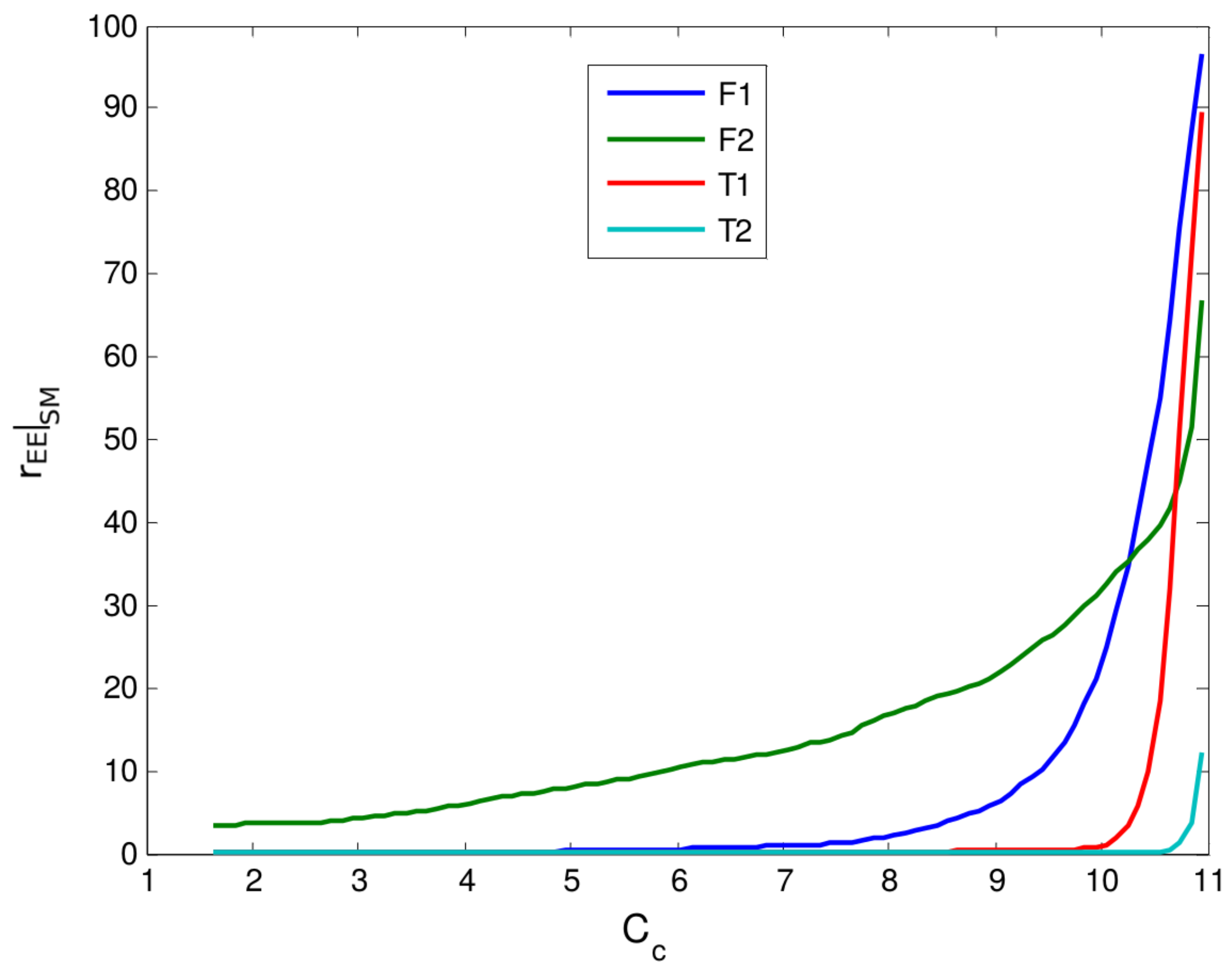
An equivalent form to obtain the effect of tolerances (as observed in Table 1 for ) consists of manipulating the critical values of acceptance, . Figure 2 shows that, given a convenient choice of critical value or its analogous , levels of stationarity for can be obtained similar to those observed in Table 1 for the RTO system (), in an equivalent form to the use of tolerances .
However, if the tolerance is used without an appropriate evaluation of the size of the data horizon, the steady-state detection might be biased towards the acceptance of stationarity. In this case, there is an increase in the inertia of transitions in detection, thus delaying changes of state. This behavior is illustrated in Figure 3, which shows successive changes in the signal of variable during a specific time interval. It can be seen that stationarity is indicated with delay, which corresponds to those moments where the signal already presents a state of reduced variability. Assuming that the visual judgment is a legitimate way of determining signal stationarity, it is clear that, in this case, dynamic data are used to update the static process model and support the determination of optimal process operating condition.
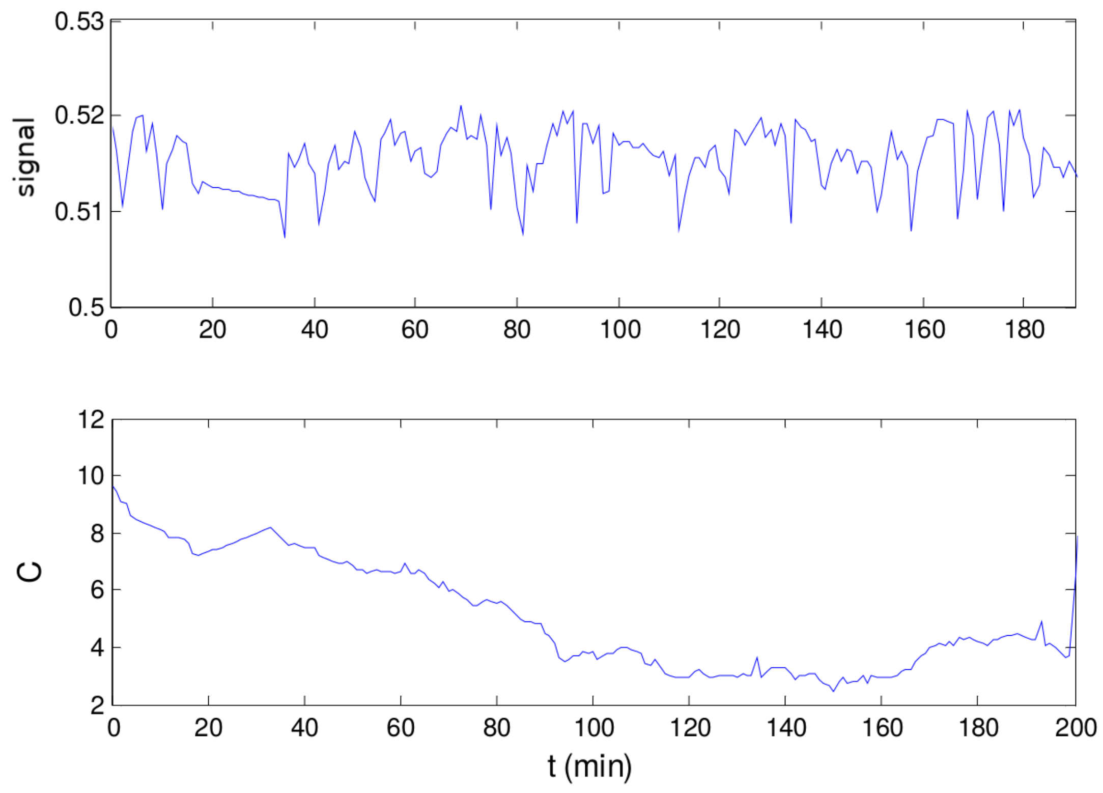
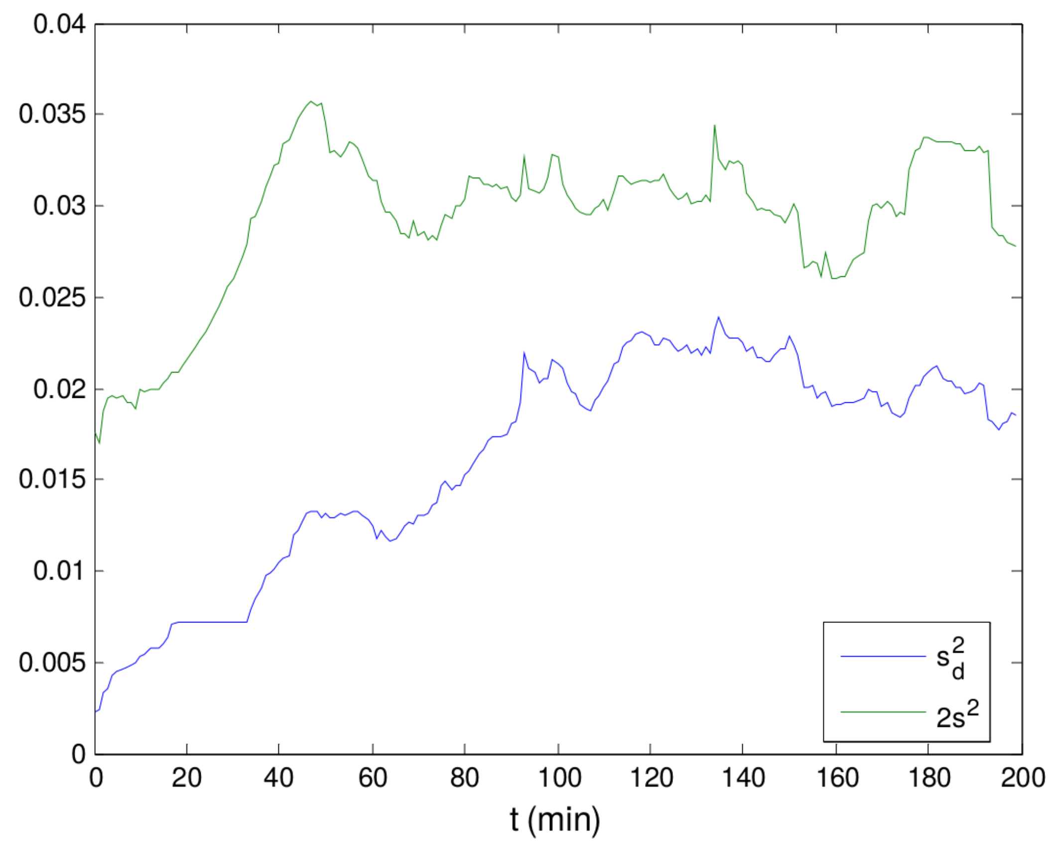
The frequency of stationarity may seem surprisingly low as pointed out by the SM in the absence of changes in tolerances and critical values. This is due to factors uncorrelated with the process, such as the sampling interval between measurements and signal conditioning filters. When this test is applied to the values from Figure 3, results reveal no stationarity at all during the period. Even more weird is that, based on a visual inspection, the values are apparently steady within the interval comprised between the beginning and ∼200 min. However, it must be noted that this method is very sensitive to short-term variability, being affected by signal preprocessing in the DCS and by the sampling interval. If one observes the signal behavior within the first 200 min with appropriate axes values, as in Figure 4, a pattern of autocorrelation can be noted, independent of the signal amplitude. The autocorrelation renders the difference between two successive points to be lower than that expected in the case of no autocorrelation, i.e., in the case that each point were due to a pure stochastic process. As a consequence, the value of (Equation (13)) decreases when compared to the variance in relation to the average. This is made clear from Figure 5, where the evolution of and along the first 200 min is depicted. Thus, the values of C are increased beyond the critical value of acceptance.
4.2. Adaptation and Optimization
The decision variables for adaptation and optimization problems, and , are selected by the user on both RTO systems. Since this choice is not based on any systematic method, it is supported by testing and experience or by the engineer/user beliefs, expectations and/or wishes. Therefore, decision variable selection is restricted to the user, and the optimizer only chooses their values.
Both commercial RTO systems discussed here make use of a recent data window in the adaptation step, which comprises a series of values along a time horizon of a certain length. The values within the moving data horizon are measurements obtained from the plant information system for each measured variable. The data window is represented as:
where and are the set of data obtained at the first and current sampling instants of the moving window by direct observation and H is the number of successive time steps uniformly separated by a sampling time of , defining a data horizon from to . Considering applications in crude oil distillation units, it is common to adopt the size of the data window as 1 h, with a sampling instant typically in the range between 0.5 and 1 min, which results in n between 120 and 60, respectively.
The model adaptation step in both RTO systems consists of a nonlinear programming model whose objective function is the weighted sum of squared errors between plant measurements and model predictions, as presented in Equation (21). The weights, , are the variances of each measurement.
It must be noted that there is an important difference between the objective function employed by Equation (21) and the maximum likelihood estimator shown in Equation (10) for Gaussian, zero mean and additive measurement errors. Both tools reduce the data window of each variable to only one value, which corresponds to the average of measurements within the window (most likely due to the easiness of implementation). In this case, the changes go beyond the apparent simplicity that such a modification may introduce to carry on the calculations. The resulting expression is not assured to hold the desired statistical properties that apply to a maximum likelihood estimator, i.e., unbiased and efficient estimations [37]. In addition, as shown in Equation (21), the elements correspond to the standard deviation of measurements. From this, the a priori assumption of independent errors is also clear, since the expression “corresponds” to a simplification of the use of a diagonal covariance matrix.
It is noted in industrial implementations that the choice of sets upd and obj (i.e., the decision vector θ and the set of variables in the objective function) is almost always based on empirical procedures. It is interesting to note that the premises that support the choices of obj set are hardly observed. According to these premises, an important element is that obj encompasses measured variables, which are non-zero values of , directly affected by the corruption of experimental signals. However, it may be seen in real RTO systems that there is the inclusion of updated parameters and non-measured variables (upd set) in the set obj. A typical occurrence of such a thing is the inclusion of load characterization parameters, which belong to the upd set and are often included in the objective function of the model adaptation problem. In this case, where there is no measured value for , fixed values are arbitrarily chosen for these variables. As a result, this practice limits the variation of these variables around the adopted fixed values. This approach degenerates the estimator and induces the occurrence of bias in estimated variables.
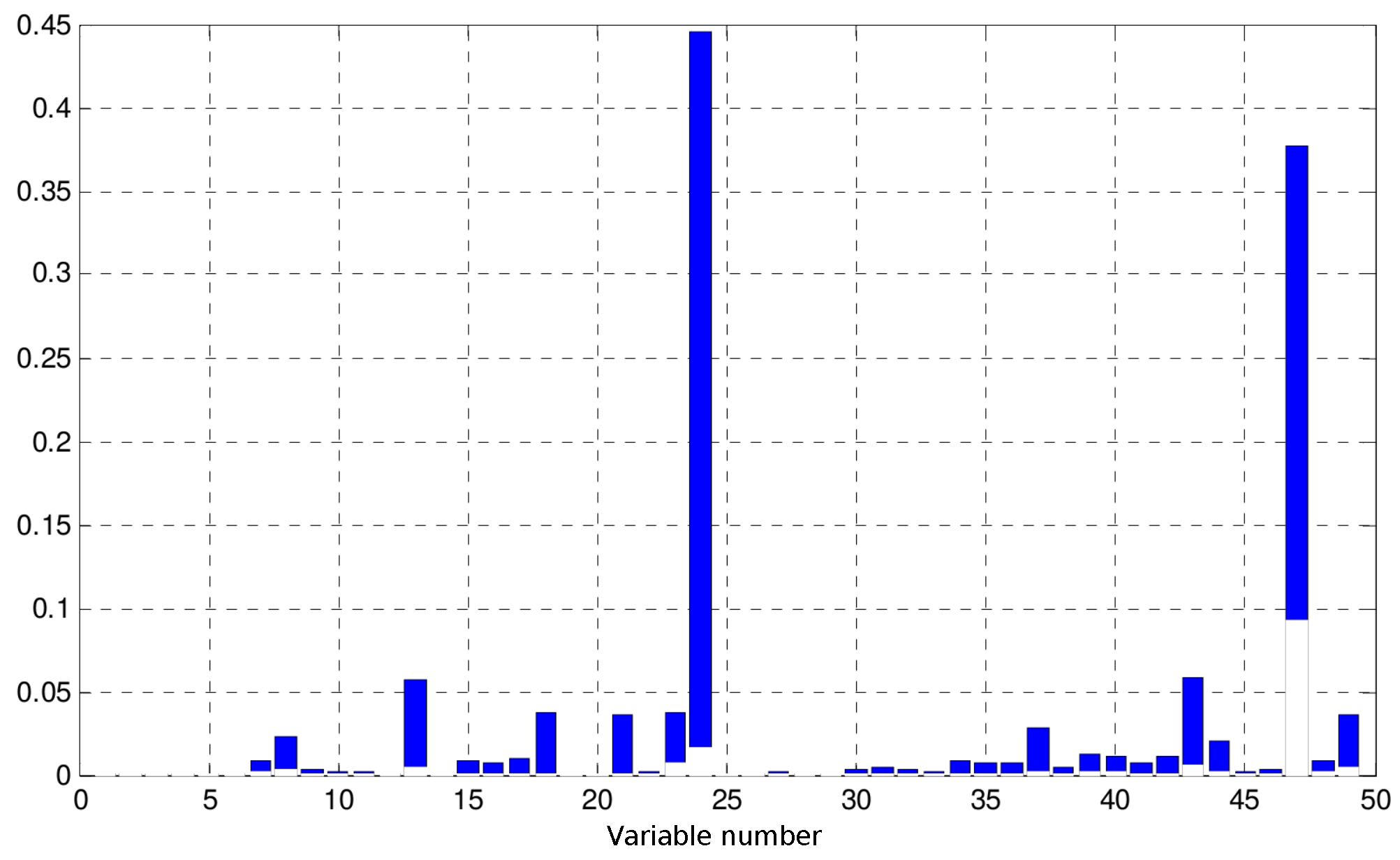
In order to take a closer look at the effects of ill-posed problems in RTO systems, we will discuss the influence of each variable in obj over the value of the objective function from Equation (21) with real RTO data. Assuming that Equation (10) is valid, measurement errors are independent and the knowledge of the true variance values for each measured variable is available, it is expected that the normalized effects, , of each variable in obj are similar, as defined in Equation (22). In Tool A, the number of variables in set obj was 49. The time interval between two successful and successive RTO iterations has a probability density with 10th, 50th and 90th percentiles of 0.80, 1.28 and 4.86, respectively. The normalized effects , as defined in Equation (22), are shown in Figure 6. Results show that it is common that fewer variables within obj have greater effects in objective function values. For a period of three months, the RTO system from Tool A has been executed 1000 times, but achieved convergence for the reconciliation and model adaptation step in 59.7% of cases. Besides the formulation of the estimation problem, this relatively low convergence rate might be caused by the following reasons: (i) the nonlinearity of the process model that may reach hundreds of thousands of equations, since the optimization of a crude oil atmospheric distillation unit is a large-scale problem governed by complex and nonlinear physicochemical phenomena; (ii) the model is not perfect, and many parameters are assumed to remain constant during the operation, which may not be the real case; such assumptions force estimations of updated parameters to accommodate all uncertainty and may result in great variability in estimates between two consecutive RTO iterations; and (iii) the limitations of the employed optimization technique, along with its parameterization; in most commercial RTO packages, sequential quadratic programming (SQP) is the standard optimization technique, as is the case for Tool A. Regarding convergence, thresholds are empirical choices, generally represented by rules of thumb.
In Table 2 are presented contribution details for variables with the 10 greatest values of the 50th percentile (median) for the considered period. The tag field indicates the nature of the variable, which may be a flow rate (F), a temperature (T) or a model parameter (θ), i.e., an unmeasured variable. Besides the comparison of the median values, the values for the 10th and 90th percentiles show greater variance in the effects of each variable. As an example, the first two variables in Table 2 vary as high as 100% among percentiles. In fact, some discrepancy among the contribution of variables in obj in objective function values is expected, as long as the variables are expressed with different units, and this effect is not fully compensated by the variances. Nevertheless, this fact does not explain the high variation along the operation, which can be attributed to the violation of one or more hypothesis in different operating scenarios. Even in this case, it is not possible to determine which assumptions do not hold.
It is not an easy task to analyze the operation of a real RTO system, since the knowledge about factors that influence and describe the plant behavior is limited. For this reason, we will put emphasis on the variability of the system’s results. In doing this, we are able to compare the frequency of the most important disturbances (such as changes in the load) with the variability presented by RTO results (such as objective function values, estimated variables and the expectancy of economic performance). In this context, it is worth assessing the behavior of estimated variables that are related to the quality of the load of the unit. In refineries, the molecular characterization of the oil is not usual. In turn, physicochemical properties are used to describe both the oil and its fractions (cuts). A common analysis is the ratio between distillation fractions and their volumetric yields, which results in profiles such as ASTM-D86 (ASTM-D86 is a standard test method for the distillation of petroleum products and liquid fuels at atmospheric pressure, which evaluates fuel characteristics, in this case, distillation features). In the conventional operation of a refinery, such profiles are not available on-line for the load, even though there are databases for oils processed by the unit. These analyses may differ from the true values due to several factors:
- the database might present lagged analyses, given the quality of oil changes with time;
- there might be changes in oil composition due to storage and distribution policies from well to final tank. Commonly, this causes the loss of volatile compounds;
- mixture rules applied to determine the properties of the load might not adequately represent its distillation profile;
- eventually, internal streams of the refinery are blended with the load for reprocessing.
Since the characterization of the load has a huge impact in determining the quality and quantity of products, these sources of uncertainty generally motivate the use of specific parameters, called knots, that are related to the fit of the distillation profile. The distillation profile is divided into sections, and each knot represents the slope coefficient of each section of the profile. These parameters are thus included in the set of estimated parameters (). In the present case, 11 knots are the degrees of freedom of the model adaptation problem and could be used to infer the quality of the load based on available measurements and the process model for the distillation column.
The estimated knots’ variability is depicted in Figure 7A by means of the distribution of estimated values for each knot, where the reference load corresponds to the knot equal to one. In addition, Figure 7B also shows the relative difference between two successive estimations of each knot. A high total variability, as well as a high amplitude for the relative difference of two successive estimations can be seen. However, considering the knowledge about the real load, such observations are incompatible with the state of the load during the operation. In the considered distillation unit, the oil load changes approximately once a week, which involves three tank transfers. Nonetheless, relative differences as high as 20% are common between two successive estimates for many knots. Considering an interval of 1.5 h between estimations, such a variability would not be expected. Besides that, as knots are independent estimates, the variation between contiguous knots might give rise to distillation profiles that do not make real physical sense.
In Table 3 are presented the lower and upper bounds applied to knots in the model adaptation problem, as well as the relative number of iterations with active constraints under convergence. From the results, one might infer that the observed variability in estimated values of knots would be higher if the bounds have allowed. These bounds deliberately force values to real physical ranges. However, this procedure alone does not guarantee real physical meaning, but only restricts the expected values to reasonable ranges. Indeed, with fewer degrees of freedom, the numerical optimization procedure would search for other “directions” to minimize the objective function, thus propagating the uncertainties to other decision variables. In summary, the approach compensates the lower flexibility to change some parameters by introducing bias in the estimates of other decision variables. Even poorer estimations, as those trapped in local minima, were further discussed in Quelhas et al. [31].
The high variability is also reflected in the values of the objective function, as can be seen in Figure 8, where the relative difference of objective function values () is shown under convergence between two successive iterations, i.e.,
In the absence of actual short-term changes in the process (i.e., between two RTO iterations), it is not easy to explain such a high variation in terms of real changes or disturbances. Reasonable explanations could be the violation of any of the hypothesis assumed for the identification problem and/or the quality of the solution given by the employed numerical optimization technique [31].
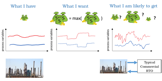
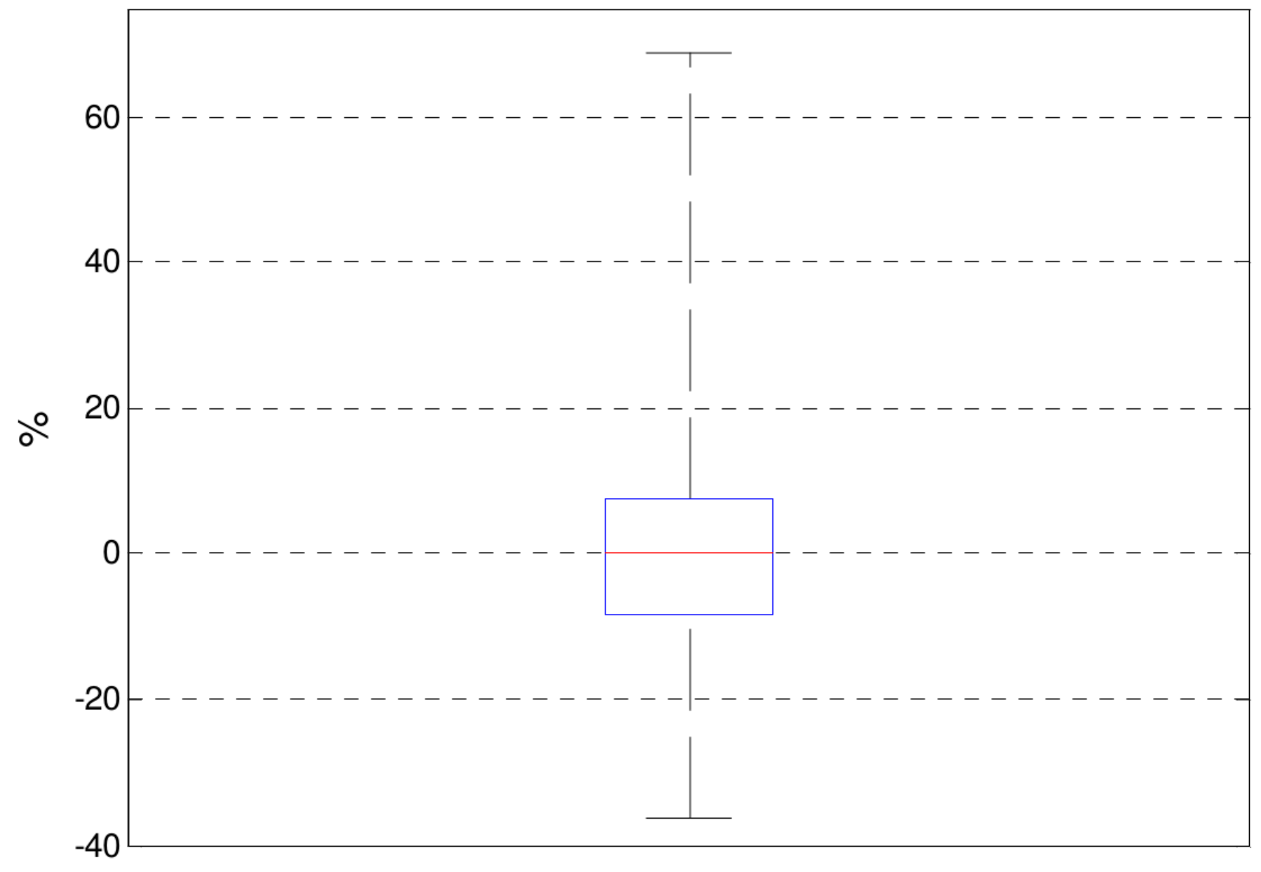
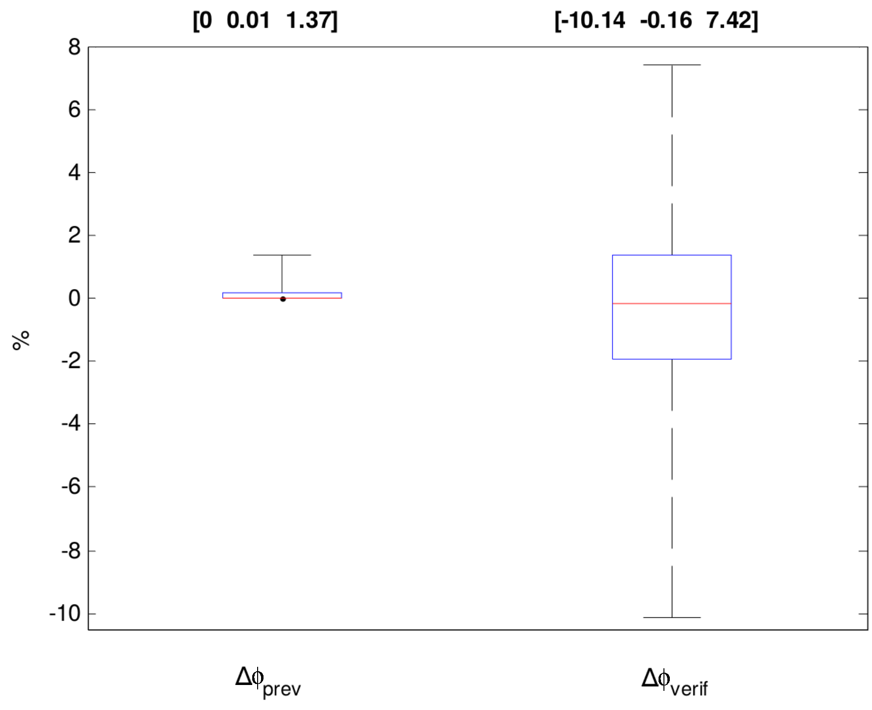
Finally, it is worth analyzing the metric of assessment of the RTO system performance. The following two performance metrics are considered: the relative difference between the calculated profit value before, , and after, , the RTO iteration k (, Equation (23)); and the relative difference between the profit value calculated at the beginning of RTO iteration k, , and the profit estimated by the previous iteration, (, Equation (24)). It must be emphasized that both metrics refer to profit estimates calculated by the RTO model, which will reflect real values only for a perfect model.
As shown in Figure 9, the most used metric of assessment of RTO performance, , has an optimistic bias, as it always reports positive values (as it should be for the converged RTO results). However, the results of , reflecting the process response over the last result, reveal that changes in decision variables are not leading to better economic performance in all RTO iterations. Even worse, they reveal the addition of useless variability to decision variables. In this context, considering the validity of the results for , it is worth noting its low value of only 0.01 for the 50th percentile. This reveals the clear need of analyzing RTO results to distinguish between statistically-significant results from those that are due to a common cause of variation [30,49,50,51]. If the dominant cause of plant variation results from the propagation of uncertainties throughout the RTO system, implementing these changes could lower profit, as is interestingly observed in the results of , confirmed by a negative 50th percentile.
5. Conclusions
The implementation of optimization procedures in real time for the improvement of processes constitutes a major challenge in real-world implementations, as is the case of RTO systems. In this context, we are compelled to confirm the quotation from Bainbridge [52] that “perhaps the final irony is that it is the most successful automated systems, with rare need for manual intervention, which may need the greatest investment in human operator training”.
This work has evaluated and analyzed the performance of RTO packages from two world-class providers running on crude oil distillation units from two different commercial-scale Brazilian petroleum refineries. We have briefly presented the steady-state detection methods available on these RTO packages and discussed the choice of the method and its parameters, the selection of measured signals to be submitted to the stationarity test and the tolerance criteria. It was shown that in spite of the methods available, some tuning parameters might compromise any statistical foundation eventually present, redefining stationarity in terms of the user’s choice without improving the global performance of RTO. Regarding model adaptation, we have examined the problem formulation, the choice of adjustable model parameters and the selection of variables in the objective function, the convergence rate of the optimization technique and the variability of estimates. It was presented that the problem formulation lacks features to ensure unbiased and efficient estimations, which contribute to the addition of useless variability to decision variables. Finally, we have analyzed economic optimization results and showed that even though the RTO system is able to find improved values for decision variables, their implementation might not lead to better economic performance as estimated by the RTO. In practice, all choices are done on a subjective basis, supported by the operating experience of engineers, as well as empirical knowledge of software vendors. As has been shown, a possible outcome is that RTO results have an optimistic bias, in which changes in decision variables are not leading to better economic performance in all RTO iterations (Figure 9).
Given the already established conditions for model adequacy within the context of the two-step approach [22], updated parameters are just mathematical tools used by the model fitting procedure to accommodate any disagreement between model predictions and plant measurements. In other words, it is assumed that all modeling uncertainties, though unknown, might be incorporated in the vector of uncertain parameters θ. Since the plant will typically not be in the set of models obtained by spanning all of the possible values of the model parameters, the two-step approach will fail in the presence of structural plant-model mismatch. However, we should ask if the structural inability of the two-step approach is the primary source of uncertainty in RTO systems. Indeed, the disagreement in the mathematical model structure is not the only source of plant-model mismatch. The fault in steady-state detection is a source of model uncertainty and not a parametric one. This is due to the fact that derivative terms are ignored. Even for methods that theoretically are not affected by plant-model mismatch, a wrong steady-state detection will negatively impact the method’s result. In addition, given the enormous amount of data and gradient estimations that would be required in a large-scale process, none of such “model-free” methods are viable for application in real industrial processes. This notwithstanding, the aforementioned disagreement may be caused by any factor that impairs information acquisition and processing in real implementations, constituting sources of uncertainty, such as: (i) measurements signals corrupted by noise with an unknown error structure; (ii) variation of the elements of input , neither measured, nor estimated (); (iii) use of the wrong default values for fixed variables; (iv) use of an inaccurate process model; (v) violation of maximum likelihood assumptions; (vi) imperfect numerical optimization method; and (vii) imperfect steady state detection or gross error filtering.
From a practical point of view, the task of diagnosing an RTO system based on the two-step approach is a challenging one. There is a very high level of uncertainty spread along all system modules. Since conclusions will likely be dependent on non-validated assumptions, the overlapping of too many possible causes of failure hampers the production of higher level diagnostics. In this context, this work illustrates some crucial features involved when evaluating RTO systems’ performance, as already discussed in detail elsewhere [31]. Some results from two industrial RTO implementations are analyzed, providing some insights on common causes of performance degradation in order to have a clearer picture of the system performance and its main drawbacks. Such an analysis is a step forward towards the proper identification of existent system vulnerabilities, so that the RTO system structure and function may be improved.
Acknowledgments
The authors thank CNPq (Conselho Nacional de Desenvolvimento Científico e Tecnológico) and CAPES (Coordenação de Aperfeiçoamento de Pessoal de Nível Superior) for the financial support to this work, as well as for covering the costs to publish in open access. The authors also thank Petrobras (Petróleo Brasileiro SA) for supporting this work.
Author Contributions
A.D.Q. gathered the data and contributed analysis tools; A.D.Q., J.C.P. and M.M.C. analyzed the data; M.M.C. and A.D.Q. wrote the paper.
Conflicts of Interest
The authors declare no conflict of interest.
Abbreviations
The following abbreviations are used in this manuscript:
| RTO | Real-time optimization systems |
| MPC | Model predictive control |
| MON | Monitoring sequence |
| SSD | Steady-state detection |
| APC | Advanced process control |
| DCS | Distributed control system |
| SM | Statistical method |
| HM | Heuristic method |
References
- Garcia, C.E.; Morari, M. Optimal operation of integrated processing systems. Part I: Open-loop on-line optimizing control. AIChE J. 1981, 27, 960–968. [Google Scholar] [CrossRef]
- Ellis, J.; Kambhampati, C.; Sheng, G.; Roberts, P. Approaches to the optimizing control problem. Int. J. Syst. Sci. 1988, 19, 1969–1985. [Google Scholar] [CrossRef]
- Engell, S. Feedback control for optimal process operation. J. Process Control 2007, 17, 203–219. [Google Scholar] [CrossRef]
- Chachuat, B.; Srinivasan, B.; Bonvin, D. Adaptation strategies for real-time optimization. Comput. Chem. Eng. 2009, 33, 1557–1567. [Google Scholar] [CrossRef]
- François, G.; Bonvin, D. Chapter One—Measurement-Based Real-Time Optimization of Chemical Processes. In Control and Optimisation of Process Systems; Advances in Chemical Engineering; Pushpavanam, S., Ed.; Academic Press: New York, NY, USA, 2013; Volume 43, pp. 1–50. [Google Scholar]
- Cutler, C.; Perry, R. Real time optimization with multivariable control is required to maximize profits. Comput. Chem. Eng. 1983, 7, 663–667. [Google Scholar] [CrossRef]
- Bamberger, W.; Isermann, R. Adaptive on-line steady-state optimization of slow dynamic processes. Automatica 1978, 14, 223–230. [Google Scholar] [CrossRef]
- Jang, S.S.; Joseph, B.; Mukai, H. On-line optimization of constrained multivariable chemical processes. AIChE J. 1987, 33, 26–35. [Google Scholar] [CrossRef]
- Arkun, Y.; Stephanopoulos, G. Studies in the synthesis of control structures for chemical processes: Part IV. Design of steady-state optimizing control structures for chemical process units. AIChE J. 1980, 26, 975–991. [Google Scholar] [CrossRef]
- Darby, M.L.; Nikolaou, M.; Jones, J.; Nicholson, D. RTO: An overview and assessment of current practice. J. Process Control 2011, 21, 874–884. [Google Scholar] [CrossRef]
- Naysmith, M.; Douglas, P. Review of real time optimization in the chemical process industries. Dev. Chem. Eng. Miner. Process. 1995, 3, 67–87. [Google Scholar] [CrossRef]
- Marlin, T.E.; Hrymak, A.N. Real-Time Operations Optimization of Continuous Processes; AIChE Symposium Series; 1971-c2002; American Institute of Chemical Engineers: New York, NY, USA, 1997; Volume 93, pp. 156–164. [Google Scholar]
- Trierweiler, J.O. Real-Time Optimization of Industrial Processes. In Encyclopedia of Systems and Control; Baillieul, J., Samad, T., Eds.; Springer: London, UK, 2014; pp. 1–11. [Google Scholar]
- Rotava, O.; Zanin, A.C. Multivariable control and real-time optimization—An industrial practical view. Hydrocarb. Process. 2005, 84, 61–71. [Google Scholar]
- Young, R. Petroleum refining process control and real-time optimization. IEEE Control Syst. 2006, 26, 73–83. [Google Scholar] [CrossRef]
- Shokri, S.; Hayati, R.; Marvast, M.A.; Ayazi, M.; Ganji, H. Real time optimization as a tool for increasing petroleum refineries profits. Pet. Coal 2009, 51, 110–114. [Google Scholar]
- Ruiz, C.A. Real Time Industrial Process Systems: Experiences from the Field. Comput. Aided Chem. Eng. 2009, 27, 133–138. [Google Scholar]
- Mercangöz, M.; Doyle, F.J., III. Real-time optimization of the pulp mill benchmark problem. Comput. Chem. Eng. 2008, 32, 789–804. [Google Scholar] [CrossRef]
- Chen, C.Y.; Joseph, B. On-line optimization using a two-phase approach: An application study. Ind. Eng. Chem. Res. 1987, 26, 1924–1930. [Google Scholar] [CrossRef]
- Yip, W.; Marlin, T.E. The effect of model fidelity on real-time optimization performance. Comput. Chem. Eng. 2004, 28, 267–280. [Google Scholar] [CrossRef]
- Roberts, P. Algorithms for integrated system optimisation and parameter estimation. Electron. Lett. 1978, 14, 196–197. [Google Scholar] [CrossRef]
- Forbes, J.; Marlin, T.; MacGregor, J. Model adequacy requirements for optimizing plant operations. Comput. Chem. Eng. 1994, 18, 497–510. [Google Scholar] [CrossRef]
- Chachuat, B.; Marchetti, A.; Bonvin, D. Process optimization via constraints adaptation. J. Process Control 2008, 18, 244–257. [Google Scholar] [CrossRef]
- Marchetti, A.; Chachuat, B.; Bonvin, D. A dual modifier-adaptation approach for real-time optimization. J. Process Control 2010, 20, 1027–1037. [Google Scholar] [CrossRef]
- Bunin, G.; François, G.; Bonvin, D. Sufficient conditions for feasibility and optimality of real-time optimization schemes—I. Theoretical foundations. arXiv 2013. [Google Scholar]
- Gao, W.; Wenzel, S.; Engell, S. A reliable modifier-adaptation strategy for real-time optimization. Comput. Chem. Eng. 2016, 91, 318–328. [Google Scholar] [CrossRef]
- Yip, W.S.; Marlin, T.E. Multiple data sets for model updating in real-time operations optimization. Comput. Chem. Eng. 2002, 26, 1345–1362. [Google Scholar] [CrossRef]
- Yip, W.S.; Marlin, T.E. Designing plant experiments for real-time optimization systems. Control Eng. Pract. 2003, 11, 837–845. [Google Scholar] [CrossRef]
- Pfaff, G.; Forbes, J.F.; McLellan, P.J. Generating information for real-time optimization. Asia-Pac. J. Chem. Eng. 2006, 1, 32–43. [Google Scholar] [CrossRef]
- Zhang, Y.; Nadler, D.; Forbes, J.F. Results analysis for trust constrained real-time optimization. J. Process Control 2001, 11, 329–341. [Google Scholar] [CrossRef]
- Quelhas, A.D.; de Jesus, N.J.C.; Pinto, J.C. Common vulnerabilities of RTO implementations in real chemical processes. Can. J. Chem. Eng. 2013, 91, 652–668. [Google Scholar] [CrossRef]
- Friedman, Y.Z. Closed loop optimization update—We are a step closer to fulfilling the dream. Hydrocarb. Process. J. 2000, 79, 15–16. [Google Scholar]
- Gattu, G.; Palavajjhala, S.; Robertson, D.B. Are oil refineries ready for non-linear control and optimization? In Proceedings of the International Symposium on Process Systems Engineering and Control, Mumbai, India, 3–4 January 2003.
- Basak, K.; Abhilash, K.S.; Ganguly, S.; Saraf, D.N. On-line optimization of a crude distillation unit with constraints on product properties. Ind. Eng. Chem. Res. 2002, 41, 1557–1568. [Google Scholar] [CrossRef]
- Morari, M.; Arkun, Y.; Stephanopoulos, G. Studies in the synthesis of control structures for chemical processes: Part I: Formulation of the problem. Process decomposition and the classification of the control tasks. Analysis of the optimizing control structures. AIChE J. 1980, 26, 220–232. [Google Scholar] [CrossRef]
- Bailey, J.; Hrymak, A.; Treiber, S.; Hawkins, R. Nonlinear optimization of a hydrocracker fractionation plant. Comput. Chem. Eng. 1993, 17, 123–138. [Google Scholar] [CrossRef]
- Bard, Y. Nonlinear Parameter Estimation; Academic Press: New York, NY, USA, 1974; Volume 513. [Google Scholar]
- Von Neumann, J.; Kent, R.; Bellinson, H.; Hart, B. The mean square successive difference. Ann. Math. Stat. 1941, 12, 153–162. [Google Scholar] [CrossRef]
- Von Neumann, J. Distribution of the ratio of the mean square successive difference to the variance. Ann. Math. Stat. 1941, 12, 367–395. [Google Scholar] [CrossRef]
- Young, L. On randomness in ordered sequences. Ann. Math. Stat. 1941, 12, 293–300. [Google Scholar] [CrossRef]
- Cao, S.; Rhinehart, R.R. An efficient method for on-line identification of steady state. J. Process Control 1995, 5, 363–374. [Google Scholar] [CrossRef]
- Cao, S.; Rhinehart, R.R. Critical values for a steady-state identifier. J. Process Control 1997, 7, 149–152. [Google Scholar] [CrossRef]
- Shrowti, N.A.; Vilankar, K.P.; Rhinehart, R.R. Type-II critical values for a steady-state identifier. J. Process Control 2010, 20, 885–890. [Google Scholar] [CrossRef]
- Bhat, S.A.; Saraf, D.N. Steady-state identification, gross error detection, and data reconciliation for industrial process units. Ind. Eng. Chem. Res. 2004, 43, 4323–4336. [Google Scholar] [CrossRef]
- Montgomery, D.C.; Runger, G.C. Applied Statistics and Probability for Engineers, 3rd ed.; John Wiley & Sons: New York, NY, USA, 2002. [Google Scholar]
- Alekman, S.L. Significance tests can determine steady-state with confidence. Control Process Ind. 1994, 7, 62–63. [Google Scholar]
- Schladt, M.; Hu, B. Soft sensors based on nonlinear steady-state data reconciliationin the process industry. Chem. Eng. Process. Process Intensif. 2007, 46, 1107–1115. [Google Scholar] [CrossRef]
- Kelly, J.D.; Hedengren, J.D. A steady-state detection (SSD) algorithm to detect non-stationary drifts in processes. J. Process Control 2013, 23, 326–331. [Google Scholar] [CrossRef]
- Miletic, I.; Marlin, T. Results analysis for real-time optimization (RTO): Deciding when to change the plant operation. Comput. Chem. Eng. 1996, 20 (Suppl. S2), S1077–S1082. [Google Scholar] [CrossRef]
- Miletic, I.; Marlin, T. On-line statistical results analysis in real-time operations optimization. Ind. Eng. Chem. Res. 1998, 37, 3670–3684. [Google Scholar] [CrossRef]
- Zafiriou, E.; Cheng, J.H. Measurement noise tolerance and results analysis for iterative feedback steady-state optimization. Ind. Eng. Chem. Res. 2004, 43, 3577–3589. [Google Scholar] [CrossRef]
- Bainbridge, L. Ironies of automation. Automatica 1983, 19, 775–779. [Google Scholar] [CrossRef]
Figure 1.
Topology of a real RTO system running in a crude oil distillation unit. MON, monitoring sequence; SSD, steady-state detection; APC, advanded process control; DCS, distributed control system.
Figure 1.
Topology of a real RTO system running in a crude oil distillation unit. MON, monitoring sequence; SSD, steady-state detection; APC, advanded process control; DCS, distributed control system.

Figure 2.
Percentage of values assumed static as a function of critical values (the analogous of as defined by Equation (13)) of the hypothesis test applied to signals of four process variables.
Figure 2.
Percentage of values assumed static as a function of critical values (the analogous of as defined by Equation (13)) of the hypothesis test applied to signals of four process variables.

Figure 3.
Normalized values of flow rate (blue line) and the corresponding indication of stationarity according to the RTO system (pink line), where one means steady and zero means unsteady.
Figure 3.
Normalized values of flow rate (blue line) and the corresponding indication of stationarity according to the RTO system (pink line), where one means steady and zero means unsteady.

Figure 4.
(A) Normalized values of flow rate , as shown in Figure 3, in restricted axes values; (B) C-statistic values for the corresponding time interval. The value of according to the method is 1.64.
Figure 4.
(A) Normalized values of flow rate , as shown in Figure 3, in restricted axes values; (B) C-statistic values for the corresponding time interval. The value of according to the method is 1.64.

Figure 5.
Evolution of and along the first 200 min for the signal depicted in Figure 3.
Figure 5.
Evolution of and along the first 200 min for the signal depicted in Figure 3.

Figure 6.
Interval between the first and third quartiles of the normalized effect of each variable within obj for the objective function from the model adaptation problem (Equation (21)). The x-axis refer to the relative position of variables in the vector obj.
Figure 6.
Interval between the first and third quartiles of the normalized effect of each variable within obj for the objective function from the model adaptation problem (Equation (21)). The x-axis refer to the relative position of variables in the vector obj.

Figure 7.
(A) Distribution of estimated values of knots; (B) distribution of the relative deviation between two successive estimations of a knot.
Figure 7.
(A) Distribution of estimated values of knots; (B) distribution of the relative deviation between two successive estimations of a knot.
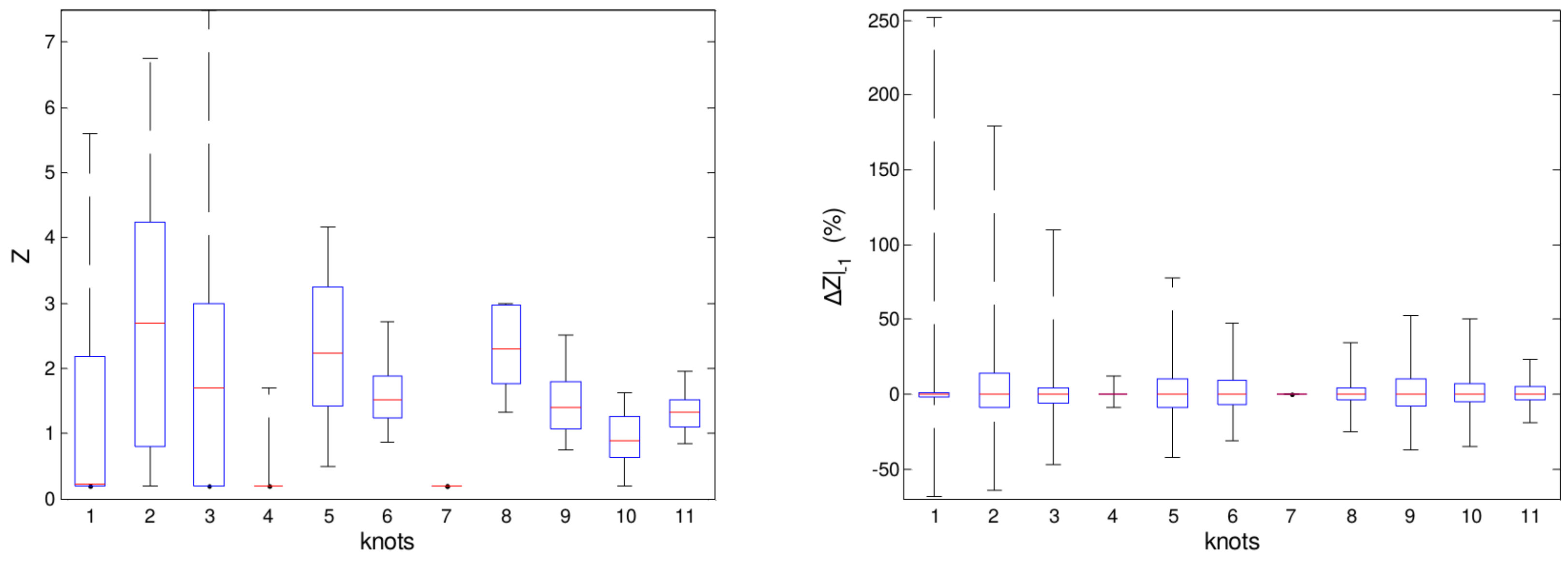
Figure 8.
Distribution of the relative difference of objective function values under convergence between two successive iterations ().
Figure 8.
Distribution of the relative difference of objective function values under convergence between two successive iterations ().

Figure 9.
Distribution of the values for and for the RTO profit. Above the graph, the percentiles P5, P50 and P95 are indicated as [P5 P50 P95].
Figure 9.
Distribution of the values for and for the RTO profit. Above the graph, the percentiles P5, P50 and P95 are indicated as [P5 P50 P95].


Table 1.
Percentage of points deemed static for the set of 8 variables. : percentage computed using results obtained by the C-statistic. : percentage computed using real results obtained by the RTO system Tool A. F, flow rate; T, temperature.
| Tag | ||
|---|---|---|
| 0.0 | 98.3 | |
| 3.2 | 81.1 | |
| 0.0 | 97.3 | |
| 0.0 | 90.9 | |
| 0.0 | 97.1 | |
| 4.8 | 99.5 | |
| 0.0 | 90.1 | |
| 6.8 | 84.4 |
Table 2.
Percentile values of normalized effects (%) of the 10 most influential variables in the value of the objective function from the model adaptation problem. The rank is relative to the 50th percentile (P50).
| Position in Rank | Tag | P50 | P90 | P10 | |
|---|---|---|---|---|---|
| 1 | yes | 21.53 | 54.83 | 1.15 | |
| 2 | yes | 15.99 | 54.33 | 0.19 | |
| 3 | yes | 2.37 | 11.39 | 0.10 | |
| 4 | yes | 1.95 | 7.49 | 0.48 | |
| 5 | yes | 1.68 | 14.21 | 0.35 | |
| 6 | yes | 1.41 | 7.01 | <0.01 | |
| 7 | yes | 1.17 | 5.94 | 0.04 | |
| 8 | yes | 1.12 | 7.39 | <0.01 | |
| 9 | θ(8) | no | 0.96 | 4.08 | 0.09 |
| 10 | yes | 0.65 | 2.17 | 0.12 |
Table 3.
Lower and upper bounds on the knots of the model adaptation problem and the percentage number of iterations in which the constraint is active under convergence.
| Knot | Active Constraint (%) | ||
|---|---|---|---|
| 1 | 0.2 | 10 | 42.5 |
| 2 | 0.2 | 10 | 13.4 |
| 3 | 0.2 | 7.5 | 31.5 |
| 4 | 0.2 | 7.5 | 81.7 |
| 5 | 0.2 | 7.5 | 0.7 |
| 6 | 0.2 | 7.5 | 0.2 |
| 7 | 0.2 | 7.5 | 92.1 |
| 8 | 0.2 | 3 | 19.4 |
| 9 | 0.2 | 3 | 1.2 |
| 10 | 0.2 | 3 | 14.6 |
| 11 | 0.2 | 3 | 0.3 |
© 2016 by the authors; licensee MDPI, Basel, Switzerland. This article is an open access article distributed under the terms and conditions of the Creative Commons Attribution (CC-BY) license (http://creativecommons.org/licenses/by/4.0/).
Share and Cite
MDPI and ACS Style
Câmara, M.M.; Quelhas, A.D.; Pinto, J.C. Performance Evaluation of Real Industrial RTO Systems. Processes 2016, 4, 44. https://doi.org/10.3390/pr4040044
AMA Style
Câmara MM, Quelhas AD, Pinto JC. Performance Evaluation of Real Industrial RTO Systems. Processes. 2016; 4(4):44. https://doi.org/10.3390/pr4040044
Chicago/Turabian StyleCâmara, Maurício M., André D. Quelhas, and José Carlos Pinto. 2016. "Performance Evaluation of Real Industrial RTO Systems" Processes 4, no. 4: 44. https://doi.org/10.3390/pr4040044
Note that from the first issue of 2016, this journal uses article numbers instead of page numbers. See further details here.