Discrete Blood Glucose Control in Diabetic Göttingen Minipigs

Abstract

Despite continuous research effort, patients with type 1 diabetes mellitus (T1D) experience difficulties in daily adjustments of their blood glucose concentrations. New technological developments in the form of implanted intravenous infusion pumps and continuous blood glucose sensors might alleviate obstacles for the automatic adjustment of blood glucose concentration. These obstacles consist, for example, of large time-delays and insulin storage effects for the subcutaneous/interstitial route. Towards the goal of an artificial pancreas, we present a novel feedback controller approach that combines classical loop-shaping techniques with gain-scheduling and modern ${\mathcal{H}}_{\infty }$-robust control approaches. A disturbance rejection design is proposed in discrete frequency domain based on the detailed model of the diabetic Göttingen minipig. The model is trimmed and linearised over a large operating range of blood glucose concentrations and insulin sensitivity values. Controller parameters are determined for each of these operating points. A discrete ${\mathcal{H}}_{\infty }$ loop-shaping compensator is designed to increase robustness of the artificial pancreas against general coprime factor uncertainty. The gain scheduled controller uses subcutaneous insulin injection as a control input and determines the controller input error from intravenous blood glucose concentration measurements, where parameter scheduling is achieved by an estimator of the insulin sensitivity parameter. Thus, only one controller stabilises a family of animal models. The controller is validated in silico with a total number of five Göttingen Minipig models, which were previously obtained by experimental identification procedures. Its performance is compared with an experimentally tested switching PI-controller.

1. Introduction

Diabetes mellitus collectively denotes a group of metabolic diseases with a worldwide increasing prevalence over the last decades. Diabetes is characterised by abnormally high blood glucose concentrations (hyperglycaemia) resulting from a dysfunction of insulin secretion, insulin action, or both [1]. In diabetes, hyperglycaemia is typically characterised by blood glucose concentrations beyond 126 mg/dL (7 mmol/L) in fasting state or beyond 200 mg/dL (11.1 mmol/L) in oral glucose tolerance tests and by increased HbA1c fraction (glycated haemoglobin >6.5%). According to a study on global estimates of diabetes prevalence [2], 382 million people in 130 countries had diabetes in 2013. This number is estimated to increase to 592 million people by 2035. A subgroup of diabetes mellitus is type 1 diabetes mellitus (T1D), which is characterised by the destruction of pancreatic β-cells (in healthy state about 65% to 80% of the islets of Langerhans) and a subsequent lack of the hormone insulin, which is important in the blood glucose regulation. About 10% of all diabetic patients are patients with T1D [3]. Diabetes might induce long term secondary diseases that may affect heart, vascular system, peripheral nervous system, and can lead to blindness, heart disease or limb amputation.

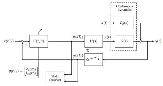
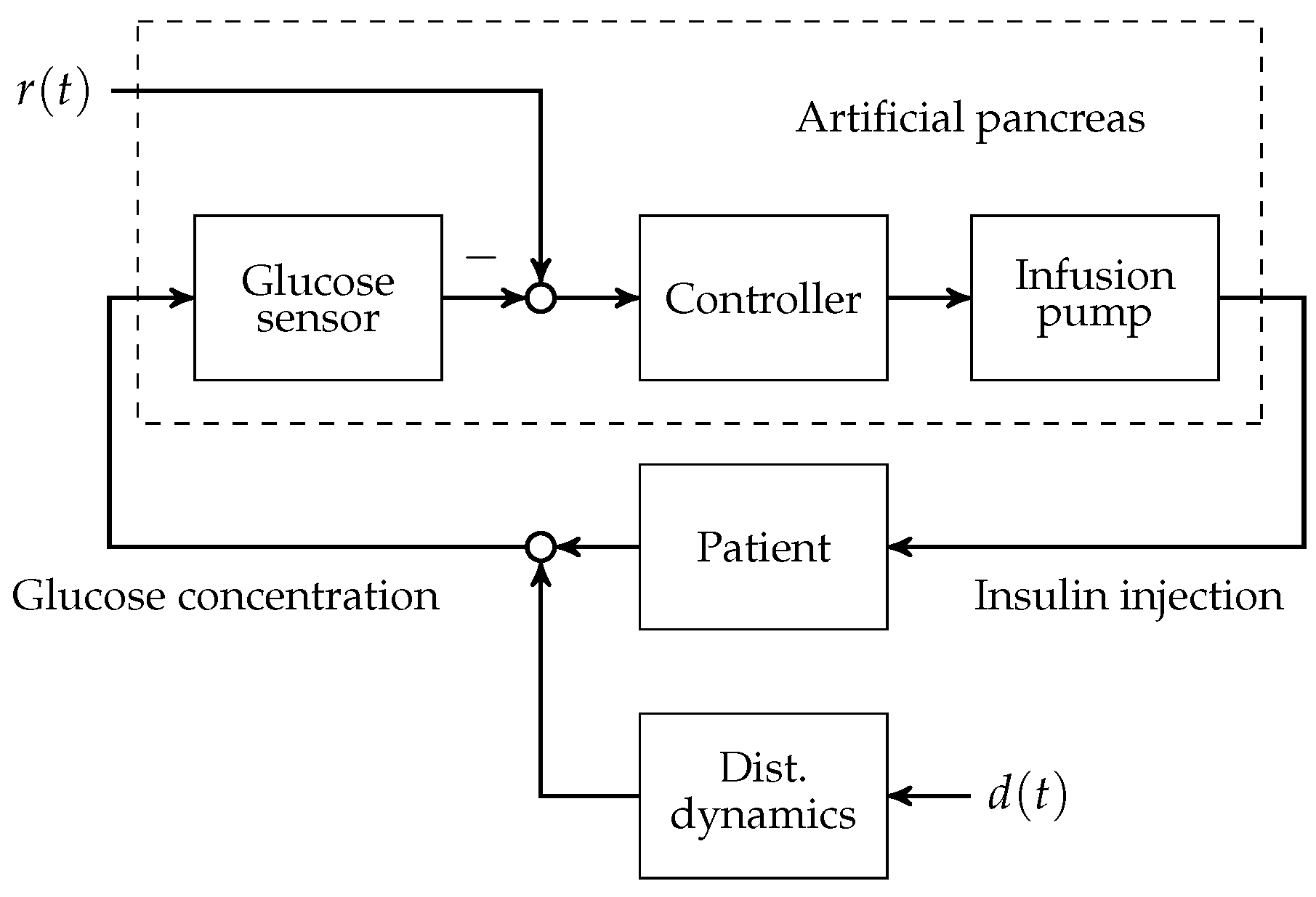
To this day, manual control has to be used for patients with T1D to reduce increased blood glucose levels to the normophysiological range. This is achieved by (a) a measurement of the blood glucose concentration; (b) the determination of an appropriate size of subcutaneously injected insulin bolus; and (c) the subcutaneous insulin injection. An overview of the feedback control system is presented in Figure 1. The patient can be seen as a feedback controller acting on its own metabolic dynamics. However, manual control of blood glucose bears several severe disadvantages. The glucose metabolic system is subject to external disturbance and internal dynamics, which affect the blood glucose level after insulin bolus application. Blood glucose predictions that are made by the patients rely heavily on expert knowledge and on sparsely available blood glucose measurements. In practice, the manual blood glucose control often leads to so-called hypo- or hyperglycaemic events. In both conditions, too low or too high blood glucose concentrations, respectively, can lead to acute problems due to too low or too high blood glucose levels.

A continuous research effort towards an automatic control of blood glucose, the so-called artificial pancreas (AP), was initiated in the early 1970s. The AP consists of three main components: (i) an insulin infusion pump; (ii) a blood glucose sensor; and (iii) a feedback control algorithm that computes insulin infusion rates based on glucose sensor measurements.

Note that other additional measurements such as meal size or physical activity might be measured and integrated into the control algorithm. An overview of the history of the AP is, for example, given in [4]. First approaches relied on intravenous blood glucose measurements and insulin application, where the main challenge is the necessary catheterisation. More recently, the subcutaneous-to-subcutaneous AP have led to a tremendous increase in research. However, this approach is associated with multiple challenges, where it is commonly agreed that a large additional time-delay in the process dynamics is most prominent. Moreover, insulin storage in the subcutaneous compartment and sudden release is associated with a variable time-delay and the risk of severe hyperinsulinaemia by some researchers [4]. A first promising scenario for the application of AP might therefore be the intensive care unit with respect to central venous catheterised patients with blood glucose imbalances [5].

Over the last three decades, a number of AP approaches were proposed by different research groups. A recent review on the state-of-the-art T1D control strategies is presented in [6]. Early controllers used, for example, proportional-integral-derivative (PID) strategies. An example is a nonlinear PD-type controller presented by Clemens [7], which was extended by moving average filtering of the measured blood glucose. However, Hernjak and Doyle [8] concluded that a simple PD controller structure is not able to stabilise the blood glucose level around a tight operating point as the nonlinear, time-varying metabolic system is subject to external disturbances. More recent approaches to AP rather focus on modern optimal or robust control methodologies [9], model predictive control (MPC) [10] or the combination of feedback and feedforward control [11,12] (which is sometimes called two-degrees-of-freedom control).

An AP should reliably stabilise the blood glucose concentration while rejecting physical activity and meal uptake metabolic disturbances with satisfactory performance. The controlled system is nonlinear, has time-varying dynamics and shows intra-individual and inter-individual parameter uncertainties. In this article, we present a novel controller design procedure that is fully discrete. In contrast to [9], our controller design procedure combines the advantages of classical frequency domain techniques with fixed structure controllers with modern internal model-based procedures for robust control, for example ${\mathcal{H}}_2$- or ${\mathcal{H}}_{\infty }$-design procedures. The central controller design is basically a discrete frequency domain disturbance rejection procedure. The design is conducted at a large number of operating points of the linearised process models. Gain scheduling of the discrete controllers is proposed on the measured blood glucose concentration and the estimated insulin sensitivity, thus guaranteeing an adaption to changing process conditions. The classical controllers are finally robustified by the discrete version of the Glover–McFarlane ${\mathcal{H}}_{\infty }$-loop-shaping procedure [13].

The AP approach in this paper is model-based and tested in an extensive in silico validation procedure with $n=5$ Göttingen Minipig models that were obtained from previously conducted animal experimental studies:

• In Section 2, we briefly describe the mathematical model of a Göttingen Minipig, which is based on the Sorensen model [14] and has already been published [15,16].
• The controller design procedure is based on the Göttingen Minipig model and is introduced in Section 3.
• Section 4 describes the animal experimental study and the results of the model identification procedure that is the basis for the controller validation.
• In Section 5, the controller performance is evaluated in silico by means of the identified animal models and compared to the performance of a structural switching P/PI-controller that was validated in vivo [17].
• Discussion of the results and a summary are given in Section 6.

2. Göttingen Minipig Model

The metabolic model of a Göttingen Minipig was adopted from the Sorensen model [14,16]. An overview of the model is presented in Figure 2. The model consists of three main subsystems: the blood circulation, the interstitium and the gastro-intestinal tract.

The models of the interstitium and the gasto-intestinal tract are interconnected via the subcutaneous insulin appearance rate $r_{ISC}\left(t\right)$ and the intravenous glucose appearance rate $r_{GGA}$ in a forward manner, respectively. External inputs to the model can be grouped into disturbances and manipulated variables. Disturbances that enter the model are the pancreatic glucagon infusion rate $S_{\Gamma }\left(t\right)=r_{P\Gamma P}^N\left(t\right)r_{P\Gamma P}^B=r_{P\Gamma P}\left(t\right)$ and orally and intravenously applied glucose rates, denoted by $D_{oral}\left(t\right)$ and $D_{iv}\left(t\right)$, respectively. The glucagon production $r_{P\Gamma P}^N\left(t\right)$ is normalised to the basal rate by $r_{P\Gamma P}^B$. Manipulated variables are the subcutaneous $U_{sc}\left(t\right)$ or the intravenous $U_{iv}\left(t\right)$ insulin infusion rates. $G_p\left(t\right)$ denotes the blood glucose concentration that is measured in the plasma.

2.1. Nonlinear State Space Model

The Göttingen Minipig model consists of $n_x=16$ first-order ordinary differential equations. The control and disturbance inputs are subsequently grouped as $\mathbf{u}\left(t\right)={[U_{\mathrm{sc}}\left(t\right),U_{\mathrm{iv}}\left(t\right)]}^T\in {\mathbb{R}}^2$ and $\mathbf{d}\left(t\right)={[D_{oral}\left(t\right),D_{iv}\left(t\right),D_{\Gamma }\left(t\right)]}^T\in {\mathbb{R}}^3$, with external glucagon infusion rate $D_{\Gamma }\left(t\right)$. With the state vector $\mathbf{x}\left(t\right)\in {\mathbb{R}}^{n_x}$ and the blood glucose concentration $y\left(t\right)=G_P\left(t\right)\in \mathbb{R}$ as system output, the nonlinear state space model is given by

$$\begin{array}{cc}\hfill \dot{\mathbf{x}}\left(t\right)& =\mathbf{f}\left(\mathbf{x}\right(t),t)+\mathbf{Bu}\left(t\right)+\mathbf{Ed}\left(t\right),\hfill \\ \hfill y\left(t\right)& ={\mathbf{c}}^T\mathbf{x}\left(t\right),\hfill \end{array}$$

(1)

where $\mathbf{f}(·):{\mathbb{R}}^{n_x}\times {\mathbb{R}}^{+}\to {\mathbb{R}}^{n_x}$ is a nonlinear smooth vector field. $\mathbf{c}$, $\mathbf{B}$ and $\mathbf{E}$ are linear mappings with according dimensions. As further simplifications, we assume that only subcutaneous insulin is available as a control input, that is $U_{\mathrm{iv}}\left(t\right)=0$. Moreover, only oral glucose disturbance $D_{oral}\left(t\right)$ is regarded in the controller design; therefore, $D_{iv}\left(t\right)=0$ and $D_{\Gamma }\left(t\right)=0$.

2.2. Model Structure

The equations of the model are derived on the basis of a compartmental modelling approach. Figure 3 gives an overview depicting an interaction diagram of a general compartment i of the model.

The mass exchange takes place between a vascular (blood) compartment V and an interstitial (bloodless) compartment I. The mass exchange in compartment i can be described by two coupled first-order differential equations

$$\begin{array}{cc}\hfill \underset{\text{mass}\text{change}}{\underbrace{V_{iV}^X·\frac{d{X}_{iV}\left(t\right)}{dt}}}& =\underset{\text{convection}}{\underbrace{Q_i^X·(X_{in}\left(t\right)-X_{iV}\left(t\right))}}-\underset{\text{diffusion}}{\underbrace{\frac{V_{iI}^X}{T_i^X}·\left(X_{iV}\left(t\right)-X_{iI}\left(t\right)\right)}},\hfill \\ \hfill \underset{\text{mass}\text{change}}{\underbrace{V_{iI}^X·\frac{d{X}_{iI}\left(t\right)}{dt}}}& =\underset{\text{diffusion}}{\underbrace{\frac{V_{iI}^X}{T_i^X}·\left(X_{iV}\left(t\right)-X_{iI}\left(t\right)\right)}}+\underset{\text{mass}\text{in-}\text{and}\text{outflow}}{\underbrace{(r_{in}\left(t\right)-r_{out}\left(t\right))}},\hfill \end{array}$$

(2)

where $X\left(t\right)$ denotes the mass distribution of a particular substance in the corresponding space. In Equation (2), $Q_i^X$ denotes the blood stream, $T_i^X$ is a time constant associated with mass diffusion and additional mass inflow and outflow are denoted by $r_{in}\left(t\right)$ and $r_{out}\left(t\right)$, respectively. The compartment i is coupled to other compartments by the mass concentration in the inflowing blood stream $X_{in}\left(t\right)$ and the mass concentration in the outflowing blood stream $X_{iV}\left(t\right)$. The blood circulation equations of the Göttingen Minipig model and corresponding parameters are not provided in this paper. Instead, the reader is referred to [15].

The dynamics of orally uptaken glucose $D_{oral}\left(t\right)$ are described by a second-order model as also presented by Hovorka et al. [18]. By denoting ${\dot{M}}_{ing,1}^G$ and ${\dot{M}}_{ing,2}^G$ the solid and the liquid glucose mass flow in the stomach and the intestine, respectively, the equations are given by

$$\begin{array}{cc}\hfill \frac{d{\dot{M}}_{ing,1}^G\left(t\right)}{dt}& =\frac{1}{T_{ing,1}}(D_{oral}\left(t\right)-{\dot{M}}_{ing,1}^G\left(t\right)),\hfill \\ \hfill \frac{d{\dot{M}}_{ing,2}^G\left(t\right)}{dt}& =\frac{1}{T_{ing,2}}({\dot{M}}_{ing,1}^G\left(t\right)-{\dot{M}}_{ing,2}^G\left(t\right)),\hfill \\ \hfill r_{GGA}\left(t\right)& =f_G{\dot{M}}_{ing,2}^G\left(t\right).\hfill \end{array}$$

(3)

In Equation (3), $T_{ing,1}$ and $T_{ing,2}$ are time constants and $f_G$ is the bioavailability of glucose in the blood.

Similar to the model of the gastro-intestinal tract, the interstitium model consists of two coupled linear differential equations of the first-order. The mass flows of nonmonomeric (inactive) insulin and monomeric (active) insulin are denoted by ${\dot{M}}_{sc,1}^I\left(t\right)$ and ${\dot{M}}_{sc,2}^I\left(t\right)$, respectively. Equations for these mass flows, that have been applied subcutaneously, are given by

$$\begin{array}{cc}\hfill \frac{d{\dot{M}}_{sc,1}^I\left(t\right)}{dt}& =\frac{1}{T_{sc,1}}\left((1-x_U)U_{sc}\left(t\right)-{\dot{M}}_{sc,1}^I\left(t\right)\right),\hfill \\ \hfill \frac{d{\dot{M}}_{sc,2}^I\left(t\right)}{dt}& =\frac{1}{T_{sc,2}}\left({\dot{M}}_{sc,1}^I\left(t\right)+x_U{U}_{sc}\left(t\right)-{\dot{M}}_{sc,2}^I\left(t\right)\right),\hfill \\ \hfill r_{ISC}\left(t\right)& ={\dot{M}}_{sc,2}^I\left(t\right),\hfill \end{array}$$

(4)

where $T_{sc,1}$ and $T_{sc,1}$ are suitable time constants and $x_U$ is a fractional parameter that is used to describe the partially activated insulin.

Note that model nonlinearities are mainly due to hyperbolic functions and bilinearities with respect to certain states [14]. In the case of the time-varying parameter insulin sensitivity $k_{IS}\left(t\right)$, the glucose concentration in the interstitium $G_{MI}\left(t\right)$ is influenced by the glucose consumption rate $r_{MGC}\left(t\right)$, which is given by

$$r_{MGC}\left(t\right)=k_{IS}\left(t\right)\left(V_{MI}^I{I}_{MI}\left(t\right)\right),$$

(5)

where $V_{MI}^I$ denotes the interstitial space for insulin and $I_{MI}\left(t\right)$ denotes the interstitial insulin concentration. The mass balance for $G_{MI}\left(t\right)$ is given by

$$V_{MI}^G\frac{d{G}_{MI}\left(t\right)}{dt}=\frac{V_{MI}^G}{T_M^G}\left(G_{MV}\left(t\right)-G_{MI}\left(t\right)\right)-r_{MGC}\left(t\right),$$

(6)

with $V_{MI}^G$ the interstitial balance volume for glucose, $T_M^G$ the diffusion time constant and $G_{MV}\left(t\right)$ the glucose concentration in the muscle and adipose tissue. A change in $k_{IS}\left(t\right)$ affects the rate of glucose consumption and increases or decreases the process gain of the blood glucose controlled plant (from $U_{sc}\left(t\right)$ to $G_p\left(t\right)$).

3. Controller Design

The controller design presented in this section is based on a model linearisation, a model reduction and a discretisation. The novel design procedure consists of a classical loop-shaping design and a subsequent ${\mathcal{H}}_{\infty }$-loop shaping robustification. To form a gain scheduling controller by lookup table interpolation, the classical loop-shaping design is presented as an automatic procedure over a large number of operating points.

3.1. Model Linearisation

The nonlinear state space model given in Equation (1) is trimmed and linearised with a first-order Taylor approximation. External disturbances and the full input vector are used in the trimming procedure. However, corresponding entries are neglected in the linearisation procedure. The trimmed dynamics result in

$$\begin{array}{cc}\hfill \mathbf{0}& =\mathbf{f}({\mathbf{x}}_{eq},t)+\mathbf{B}{\mathbf{u}}_{eq}+\mathbf{E}{\mathbf{d}}_{eq},\hfill \\ \hfill y& ={\mathbf{c}}^T{\mathbf{x}}_{eq},\hfill \end{array}$$

(7)

where the linearised state space model with state vector $\Delta \mathbf{x}$, no external disturbances $\mathbf{d}=\mathbf{0}$ and an input consisting only of subcutaneous insulin $\Delta u$ is given by

$$\begin{array}{cc}\hfill \mathcal{S}& :\left\{\begin{array}{cc}\hfill \Delta \dot{\mathbf{x}}& ={\mathbf{A}}_{eq}\Delta \mathbf{x}+\mathbf{b}\Delta u,\Delta \mathbf{x}\left(0\right)=\Delta {\mathbf{x}}_0,\hfill \\ \hfill \Delta y& ={\mathbf{c}}^T\Delta \mathbf{x},\hfill \end{array}\right.\hfill \end{array}$$

(8)

with the initial state vector $\Delta {\mathbf{x}}_0$ and $({\mathbf{A}}_{eq},\mathbf{b},\mathbf{c})$ given by the corresponding Jacobians. The model is trimmed over a range of blood glucose operating points $G_p$ and insulin sensitivity values $k_{IS}$. The set of blood glucose operating points is given by $G_p\in [50+i·20]$ mg/dL, $i\in [0,n_G-1]\subseteq \mathcal{X}\subset {\mathbb{N}}^0$. Insulin sensitivities were varied in $k_{IS}\in [0.4+j·0.2]$ mg/(min mU), $j\in [0,n_k-1]\subseteq \mathcal{Y}\subset {\mathbb{N}}^0$. $\mathcal{X}$ and $\mathcal{Y}$ denote the integer sets of blood glucose and insulin sensitivity operating points, respectively. A total of 256 models are linearised for $n_G=16$ and $n_k=16$, which are collected in set of plants

$$\mathcal{P}=\left\{{\mathcal{S}}_{ij}:i\in \mathcal{X},j\in \mathcal{Y}\right\}.$$

(9)

From the trimming procedure, the disturbance dynamics are obtained by linearisation around the same operating points. The linearised state space model with state $\Delta {\mathbf{x}}_d$ is given by

$$\begin{array}{cc}\hfill {\mathcal{S}}_d& :\left\{\begin{array}{cc}\hfill \Delta {\dot{\mathbf{x}}}_d& ={\mathbf{A}}_{d,eq}\Delta {\mathbf{x}}_d+\mathbf{e}\Delta d,\Delta {\mathbf{x}}_d\left(0\right)=\Delta {\mathbf{x}}_{d,0},\hfill \\ \hfill \Delta y_d& ={\mathbf{c}}_d^T\Delta {\mathbf{x}}_d,\hfill \end{array}\right.\hfill \end{array}$$

(10)

which are collected in the set of disturbance dynamics

$${\mathcal{P}}_d=\left\{{\mathcal{S}}_{d,ij}:i\in \mathcal{X},j\in \mathcal{Y}\right\}.$$

(11)

3.2. Discrete Controller Design Prerequisites

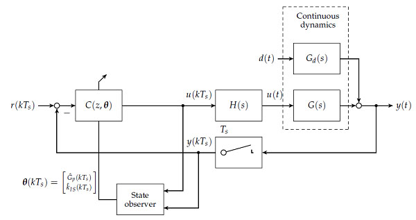
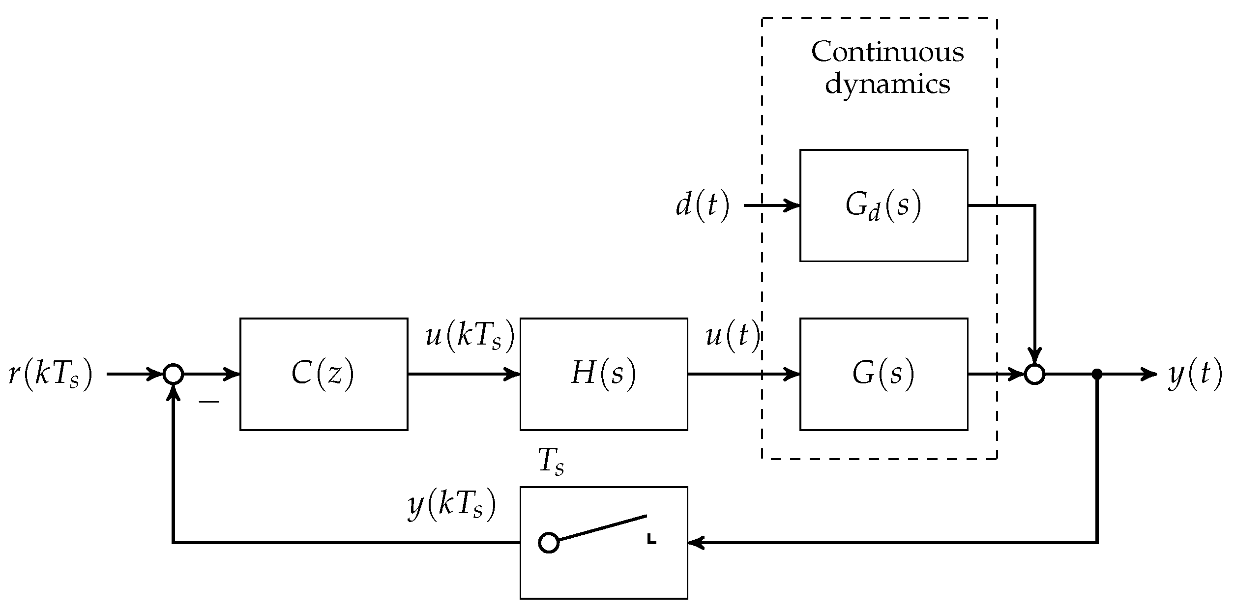
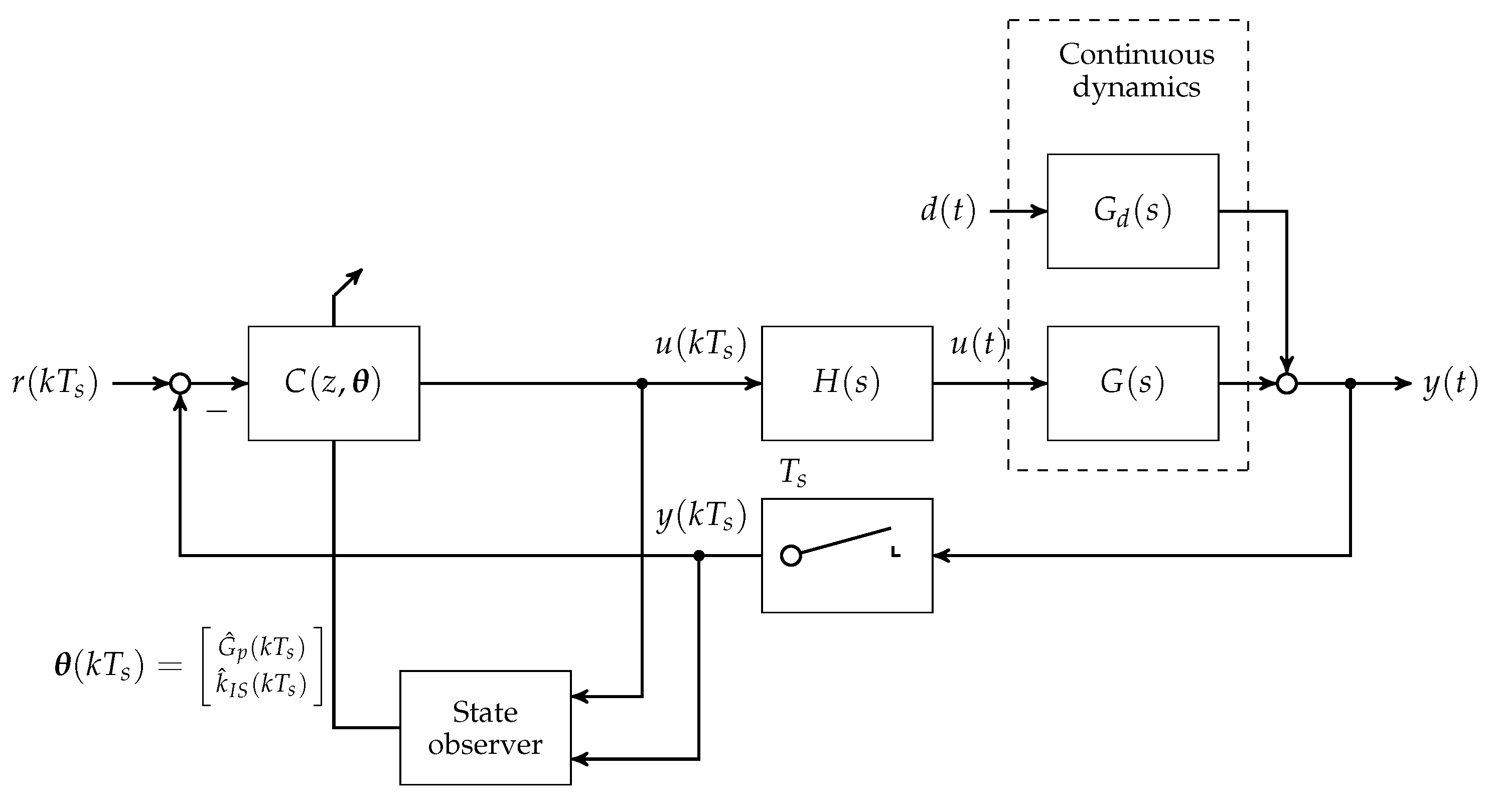
In the first step, the set of plants $\mathcal{P}$ and ${\mathcal{P}}_d$ are discretised at a sampling time of $T_s=15$ min. A block diagram showing the loop structure is given in Figure 4.

Note that $T_s$ is chosen in accordance to the animal experimental study presented in Section 4. With respect to the linearised state space models given in minimum realisation

$$G\left(s\right)\stackrel{s}{=}\left[\begin{array}{cc}{\mathbf{A}}_{eq}& \mathbf{b}\\ {\mathbf{c}}^T& 0\end{array}\right],G_d\left(s\right)\stackrel{s}{=}\left[\begin{array}{cc}{\mathbf{A}}_{d,eq}& \mathbf{e}\\ {\mathbf{c}}_d^T& 0\end{array}\right],$$

(12)

the discrete realisation of the plant is given by

$$G\left(z\right)=H_0{G}_z\left(z\right)=\frac{z-1}{z}\mathcal{Z}\left\{\frac{G\left(s\right)}{s}\right\},$$

(13)

where $H_0=H$ denotes a zero-order hold element (Figure 4) and $\mathcal{Z}\left\{·\right\}$ is the z-transform $Ƶ\left\{·\right\}$ of the δ-sampled impulse response series

$$\mathcal{Z}\left\{·\right\}=Ƶ\left\{{\mathcal{L}}^{-1}{\left.\left\{·\right\}\right|}_{t=k{T}_s}\right\},$$

(14)

with the inverse Laplace-transform ${\mathcal{L}}^{-1}\left\{·\right\}$. The disturbance transfer function is discretised by applying the z-transform to the impulse response of the disturbance dynamics

$$G_d\left(z\right)=Ƶ\left\{{\mathcal{L}}^{-1}{\left.\left\{G_d\left(s\right)\right\}\right|}_{t=k{T}_s}\right\},$$

(15)

which corresponds to an impulse-invariant discretisation. After obtaining the discretised state space realisations $G\left(z\right)$ and $G_d\left(z\right)$, the orders are subsequently reduced. Towards this end, $G\left(z\right)$ and $G_d\left(z\right)$ are brought to a balanced realisation by employing the state transformation $\overline{\mathbf{x}}=\mathbf{T}\mathbf{x}$ [19], with respect to the discete-time controllability ${\mathbf{W}}_c$ and observability ${\mathbf{W}}_o$ gramians

$${\overline{\mathbf{W}}}_c={\mathbf{T}}^{-1}{\mathbf{W}}_c{\mathbf{T}}^{-T},{\overline{\mathbf{W}}}_o={\mathbf{T}}^T{\mathbf{W}}_o,\mathbf{T},$$

(16)

where $\mathbf{T}$ is chosen such that

$${\overline{\mathbf{W}}}_c={\overline{\mathbf{W}}}_o=\Lambda .$$

(17)

In Equation (17), Λ denotes a diagonal matrix filled with (positive) square roots of the eigenvalues of ${\mathbf{W}}_c{\mathbf{W}}_o$

$$\Lambda =\mathrm{diag}\left\{{\lambda }_j^{1/2}\left({\mathbf{W}}_c{\mathbf{W}}_o\right)\right\}.$$

(18)

Consequently, balanced realised systems $\overline{G}\left(z\right)$ and ${\overline{G}}_d\left(z\right)$ are reduced to ${\widehat{G}}^r\left(z\right)$ and ${\widehat{G}}_d^r\left(z\right)$, respectively, by truncation of all states that do not correspond to the maximum eigenvalue in Λ. The resulting discrete transfer functions are given by

$${\widehat{G}}^r\left(z\right)=-\frac{b_0}{z-a_0},{\widehat{G}}_d^r\left(z\right)=\frac{b_{d,0}}{z-a_{d,0}},$$

(19)

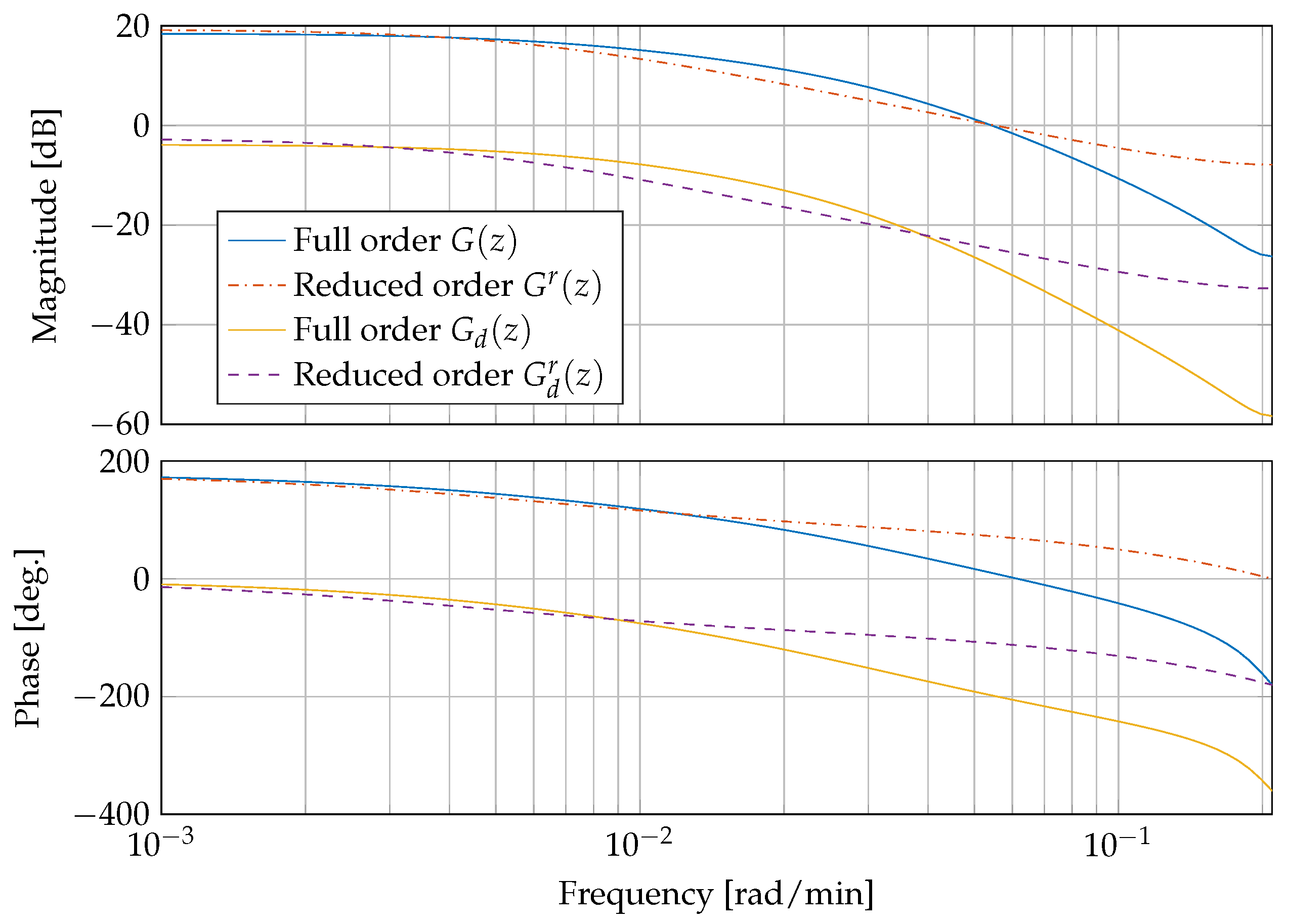
with positive constants $b_0$, $a_0$, $b_{d,0}$ and $a_{d,0}$. Figure 5 shows a comparison of the linearised and discretised full order systems $\overline{G}\left(z\right)$ and ${\overline{G}}_d\left(z\right)$ and the reduced order systems ${\widehat{G}}^r(z$ and ${\widehat{G}}_d^r\left(z\right)$. The systems correspond to a blood glucose concentration of $G_p\left(t\right)=50$ mg/dL and an insulin sensitivity of $k_{IS}\left(t\right)=0.4$ mg/(min mU).

3.3. Disturbance Rejection Design

This section presents the classical loop-shaping controller for disturbance rejection design. The presented procedure consists of three design stages, which are automatically computed over a large operating range of linearised and discretised models. A series interconnection of controllers $C_1\left(z\right)$, $C_2\left(z\right)$ and $C_3\left(z\right)$, as a result of the three design stages, forms the classical loop-shaping controller.

3.3.1. Initial Controller Gain for Disturbance Rejection

The controller is designed for disturbance rejection. Therefore, the reference input is set to zero, $r\left(k{T}_s\right)=0$ (see Figure 4). Remaining control loop inputs and outputs are scaled with respect to their maximum possible (expected) magnitudes [20]. Scaling factors are introduced for the error $d_e=e_{max}$, the process input $d_u=u_{max}$ and the disturbance input $d_d=d_{max}$. The scaled and discretised plant of reduced order $G_d^r\left(z\right)$ and the scaled and discretised disturbance process of reduced order $G_d^r\left(z\right)$ are then given by

$$G^r\left(z\right)=d_e^{-1}{\widehat{G}}^r\left(z\right)d_u,G_d^r\left(z\right)=d_e^{-1}{\widehat{G}}_d^r\left(z\right)d_d.$$

(20)

With respect to the discrete time disturbance signal $d\left(z\right)$ and the error of the control loop $e\left(z\right)=y\left(z\right)$, the objective of the controller is

$$\left|e\left(e^{j\omega T_s}\right)\right|<1,\text{assuming}\left|d\left(e^{j\omega T_s}\right)\right|<1,\forall \omega \in \left[0,\frac{{\omega }_s}{2}\right],$$

(21)

with ${\omega }_s=2\pi /T_s$. Assuming a worst case disturbance of $\left|d\right(e^{j\omega T_s}\left)\right|=1$ for some frequency ω, one can obtain

$$\left|S\left(e^{j\omega T_s}\right)G_d^r\left(e^{j\omega T_s}\right)\right|<1,\forall \omega \in \left[0,\frac{{\omega }_s}{2}\right],$$

(22)

which can be rewritten by introducing the sensitivity transfer function as $S\left(z\right)=1/(1+L(z\left)\right)$, with $L\left(z\right)=G^r\left(z\right)C\left(z\right)$. The requirement for disturbance rejection thus follows as

$$\left|1+L\left(e^{j\omega T_s}\right)\right|>\left|G_d^r\left(e^{j\omega T_s}\right)\right|,\forall \omega \in \left[0,\frac{{\omega }_s}{2}\right].$$

(23)

For frequencies ω with $|G_d^r\left(e^{j\omega T_s}\right)\left)\right|>1$, it follows that $|L\left(e^{j\omega T_s}\right)\left)\right|\gtrsim |G_d^r\left(e^{j\omega T_s}\right)\left)\right|$. The initial controller should, therefore, satisfy the following gain requirement

$$\left|C_1\left(e^{j\omega T_s}\right)\right|\ge \left|C_{min}\left(e^{j\omega T_s}\right)\right|\approx \left|\frac{G_d^r\left(e^{j\omega T_s}\right)}{G^r\left(e^{j\omega T_s}\right)}\right|.$$

(24)

It follows from Equation (19) that the initial controller is given by

$$C_1\left(z\right)=-\frac{b_{d,0}^s}{b_0^s}\frac{z-a_0}{z-a_{d,0}},$$

(25)

where the superscript s denotes the parameters of the scaled transfer functions.

3.3.2. Integral Action

In the second design phase, the initial controller is extended with integral action to reduce the remaining steady-state error of the disturbance rejection. A PI-controller $C\left(s\right)=K_p+K_i/s$ with proportional gain of $K_p=1$ is discretised by using the Tustin approximation. With $s\approx \frac{2}{T_s}\frac{z-1}{z+1}$, the discrete PI-controller is given by

$$C_2\left(z\right)=\frac{(1+\frac{K_i}{2}{T}_s)z+\frac{K_i{T}_s}{2}-1}{z-1}.$$

(26)

The value of $K_i$ is determined by employing the phase margin. Candidate integral gains $K_{i_n}$ are obtained in the log space by the set

$$K=\left\{K_{i_n}:{10}^y,y=\frac{n_1-n_0}{N-1}n+n_0,n\in \left[0\dots (N-1)\right]\right\},$$

(27)

with the initial, possibly negative exponent $n_0\in \mathbb{Z}$, the maximum exponent $n_1\in \mathbb{Z}$ and the number $N\in {\mathbb{N}}^{+}$ of candidate integral gains to be evaluated. The phase margin $P{M}_n$ is then determined over the set of candidate gains $\mathcal{K}$ for the full order open-loop compensated plant

$$P{M}_n=\angle {\left.G\left(e^{j{\omega }_{PM}{T}_s}\right)C_1\left(e^{j{\omega }_{PM}{T}_s}\right)C_2\left(e^{j{\omega }_{PM}{T}_s}\right)\right|}_{K_{i_n}\in \mathcal{K}}+{180}^{\circ },$$

(28)

where the largest gain $K_{i_n}$ with a minimum phase margin of $P{M}_n>{30}^{\circ }$ was chosen. The resulting controller has a relatively large bandwidth but an insufficiently low gain margin.

3.3.3. Lead–Lag Compensator

The third and final step of the classical loop-shaping procedure therefore consists of the design of a lead-lag compensator to increase the phase margin. A Tustin approximated lead-lag discrete compensator is used that has the form

$$C_3\left(z\right)=\frac{(2{\tau }_{LL}+T_s)z+(T_s-2{\tau }_{LL})}{(2{\tau }_{LG}+T_s)z+(T_s-2{\tau }_{LG})}.$$

(29)

Time constants ${\tau }_{LL}$ and ${\tau }_{LG}$ correspond to the lead and the lag pole, respectively. By denoting the frequency of the previously determined phase margin of Equation (28) ${\omega }_{PM}$, the time-constant of the lead part is set ${\tau }_{LL}=1/(0.7{\omega }_{PM})$. Furthermore, the time-constant of the lag part is set to ${\tau }_{LG}=2*{\tau }_{LL}$. The maximum phase increase occurs at ${\omega }_{PM}$ with a positive phase of $\approx 19.4^{\circ }$. Note that the phase margin is increased by this value. However, the GM is reduced by the additional increase in gain. The classical loop-shaping procedure is repeatedly executed over the whole set of plants $\mathcal{P}$ and ${\mathcal{P}}_d$. Hence, the total number of 256 controllers for each $C_1\left(z\right)$, $C_2\left(z\right)$ and $C_3\left(z\right)$ are determined automatically over the whole range of sampled operating points.

3.4. Robust Loop-Shaping ${\mathcal{H}}_{\infty }$-Controller

The robust loop-shaping ${\mathcal{H}}_{\infty }$-controller follows the approach of Walker [13] and increases the robustness of the shaped loop with regard to discrete, not further specified, right coprime factor uncertainty. Given the discrete compensated plant in a normalised right coprime factorisation

$$L\left(z\right)=G\left(z\right)C_1\left(z\right)C_2\left(z\right)C_3\left(z\right)=N\left(z\right)M^{-1}\left(z\right),$$

(30)

a family of coprime factor uncertain plants can be described by

$${\mathcal{P}}_{ϵ}=\left\{(N\left(z\right)+{\Delta }_M\left(z\right)){(M\left(z\right)+{\Delta }_N\left(z\right))}^{-1}:{∥{\Delta }_M\left(z\right){\Delta }_N\left(z\right)∥}_{\infty }<ϵ\right\},$$

(31)

where $\left[{\Delta }_M{\Delta }_N\right]$ provide a fairly general type of dynamic uncertainty, which allows both poles and zeros to cross out of the unit circle in the z-domain. For the generalised plant P(z) given in the form of a normalised left coprime factorisation

$$P\left(z\right)=\left[\begin{array}{cc}{P}_{11}\left(z\right)& P_{12}\left(z\right)\\ P_{21}\left(z\right)& P_{22}\left(z\right)\end{array}\right]=\left[\begin{array}{ccc}0& M^{-1}\left(z\right)& M^{-1}\left(z\right)\\ 1& N\left(z\right)M^{-1}\left(z\right)& -N\left(z\right)M^{-1}\left(z\right)\end{array}\right],$$

(32)

the application of the small gain theorem (see for example [21])

$${∥{(M\left(z\right)+K\left(z\right)N\left(z\right))}^{-1}[-K\left(z\right)-1]∥}_{\infty }\le \frac{1}{ϵ}$$

(33)

ensures robust stability with respect to the normalised coprime factor perturbed family of plants ${\mathcal{P}}_{ϵ}$. Here, the optimal achieved performance by the ${\mathcal{H}}_{\infty }$-norm $\gamma =1/ϵ$ provides a measure of tolerable right coprime factor with respect to Equation (31). An internally stabilising controller is obtained given a minimal discrete state space realisation of $P\left(z\right)$ and the solution of an indefinite discrete time algebraic Riccati equation. The central loop-shaping ${\mathcal{H}}_{\infty }$-controller $K\left(z\right)$ is employed in the overall mixed classical-robust controller

$$C_{\infty }\left(z\right)=C_1\left(z\right)C_2\left(z\right)C_3\left(z\right)K\left(z\right).$$

(34)

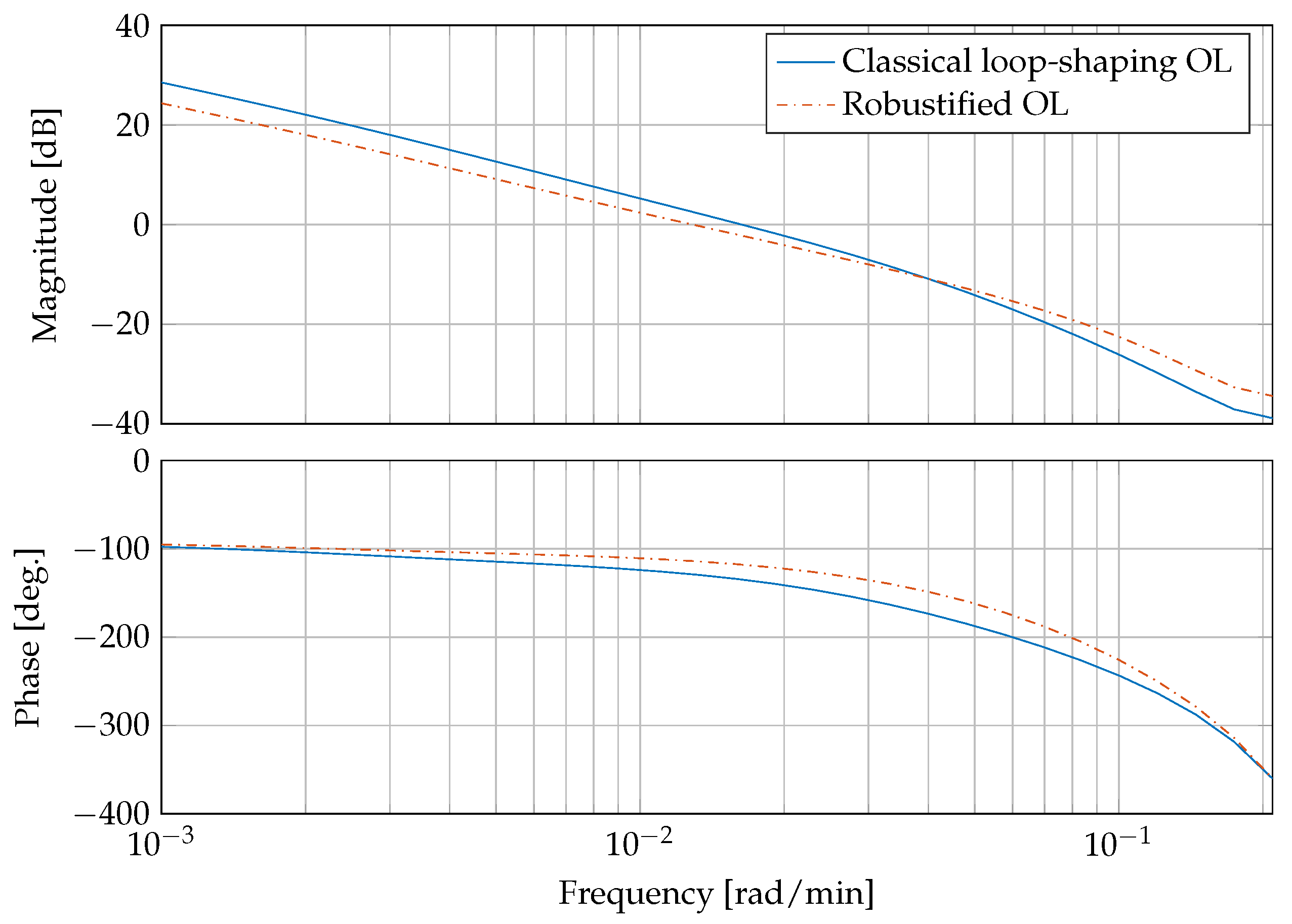
Figure 6 presents a bode plot comparing the open compensated loop with the classical controllers $L\left(z\right)$ from Equation (30) and the compensated loop with the robust controller $L_{\infty }\left(z\right)=G\left(z\right)C_{\infty }\left(z\right)$. It can be clearly seen that the gain and phase margins are increased from ${GM|}_{L\left(z\right)}=12.4$ dB and ${PM|}_{L\left(z\right)}=45.3^{\circ }$ with the classical loop-shaping controller to ${GM|}_{L_{\infty }\left(z\right)}=16.1$ dB and ${PM|}_{L_{\infty }\left(z\right)}=66.2^{\circ }$ by the robustifying approach, respectively.

This corresponds to a reduction of peak sensitivity measure $M_S={∥S\left(z\right)∥}_{\infty }$, with $S\left(z\right)=1/(1+L(z\left)\right)$. The peak sensitivity measure is reduced from $M_S{|}_{L\left(z\right)}=4.7$ dB to $M_S{|}_{L_{\infty }\left(z\right)}=2.28$ dB. An $ϵ=0.5235$ was accomplished by the the robustification procedure.

Note that only one robust ${\mathcal{H}}_{\infty }$-compensator is designed. For the design, a model at an operating point corresponding to a blood glucose concentration of $G_p\left(t\right)=130$ mg/dL and an insulin sensitivity of $k_{IS}\left(t\right)=2.0$ mg/(min mU) is chosen. Stability is determined by analysing classical gain and phase margin, as well as sensitivity peak measure $M_S$ at every operating point of $\mathcal{P}$. The resulting minimum gain and phase margin are computed as ${GM|}_{L_{\infty }\left(z\right),min}=14.2$ dB and ${PM|}_{L_{\infty }\left(z\right),min}=63.6^{\circ }$. The maximum sensitivity peak was determined as $M_S{|}_{L_{\infty }\left(z\right)}=3.1$ dB. As a consequence, it is concluded that only one ${\mathcal{H}}_{\infty }$-compensator is enough to robustly stabilise the set of plants $\mathcal{P}$. Note that an additional sensor time-delay of about 2 min was neglected in the control design prodecure, as it was considered to be sufficiently small in comparison to the sampling time of 15 min. The additional time-delay is due to the time it takes from withdrawing venous blood until a sensor value is obtained. At the crossover frequency of the compensated open-loop of 0.02 rad/min, the time-delay leads to an additional phase lag of −2.3 deg.

4. Animal Experimental Study and Model Identification

4.1. Experimental Animal Study

To identify a realistic process and for the first test of a switching PI controller, an experimental animal study was conducted (the experimental study was approved by the State Agency for Nature, Environment and Consumer Protection, North Rhine-Westphalia, Germany) with Göttingen minipigs. A total number of eight animals were included in the study that were aged 2–3 years and weighted 40–70 kg upon arrival [17]. The animals were acclimatised to standardised conditions of the animal housing in the first three weeks. Each animal was equipped with two central venous lines (Cavafix Certo 475, B.Braun Melsungen AG, Melsungen, Germany), which were implanted into the right jugular vein. An acute diabetes was induced according to the protocol of Strauss et al. [22]. During this procedure, the β-cell toxin streptozotocin (#S0130, Sigma-Aldrich, St. Louis, MO, USA or #572201 Streptozotocin, Merck Millipore, Darmstadt, Germany) was applied to the animals followed by an intensive care phase of 36 h. After 10 additional days of convalescence, glucose and insulin tolerance tests were conducted. During glucose control tests, blood glucose was measured intravenously with a minimum time interval of $T_s$. For this, 1 mL blood with no pre-treatment was withdrawn from the venous line and applied to a blood gas analyser (ABL 810 Flex, Radiometer Medical ApS, Herlev, Denmark). Short acting insulin (Humalog 100 U/mL, Lilly, Bad Homburg, Germany) was applied subcutaneously with a commercially available insulin pump (AccuCheck Combo Spirit, Roche Diagnostics, Rotkreutz, Switzerland). After euthanization, the pancreas was removed from the animals and histologically analysed by means of standard haematoxylin-eosin immunohistochemistry. An anti-insulin antibody (#IR002, Polyclonal Guinea Pig Anti-Insulin, Dako, Germany) was applied showing that only a small number of β-cells survived (5–50 cells per standardised area), compared to the reference pig (600–2800 cells per standardised area).

4.2. Model Identification

For each of the five minipigs, one parameter set could be identified, resulting in five individualised mathematical minipig models. Details on the model adaption are given in [16]. Parameters of the minipig model are partially transferred from the Sorensen model, in cases where human and animal metabolism is similar. However, a remaining set of 14 parameters was determined in a mathematical identification procedure. These parameters were determined from the minimisation of the cost function J

$$J=\underset{\mathbf{p}}{min}\sqrt{{\int }_{t_0}^{t_{end}}{e}^2(\mathbf{p},\tau )d\tau },$$

(35)

where the error $e(\mathbf{p},t)=G_{P,sim}(\mathbf{p},t)-G_{P,meas}\left(t\right)$ is computed from a comparision between in silico $G_{P,sim}(\mathbf{p},t)$ and in vivo $G_{P,sim}(\mathbf{p},t)$ blood glucose values. $\mathbf{p}\in {\mathbb{R}}^{14}$ denotes the parameter vector. To reduce the parameter space, the parameter vector is divided into five subgroups $\mathbf{p}={[{\mathbf{p}}_1^T,\dots ,{\mathbf{p}}_5^T]}^T$, the values of which were determined according to Equation (35). The corresponding experimental tests included intravenous and oral glucose applications, intravenous and subcutaneous insulin injections, and glucose concentration measurements. The identification process was implemented in MATLAB using the Levenberg–Marquardt optimisation algorithm (lsqnonlin, Optimisation Toolbox, The MathWorks, Natick, MA, USA). Figure 7 shows a comparison of in vivo data with results of the model identification procedure.

In the experiment, intravenous glucose was administered at $t=0$ min followed by two consecutive intravenous insulin impulses at $t=210$ min and $t=334$ min. In silico results evidently capture the real-life dynamics with high accuracy with respect to $\pm 10$% relative sensor error (red area in the figure). Similar results were obtained with other minipig models [15].

5. In Silico Feedback Control Study

In this section, the robust disturbance rejection control is implemented as a gain scheduled controller and tested in silico with the five minipig models. The controller performance is compared against the performance of a classical switched PI-controller that has already been tested in vivo with the diabetic Göttingen Minipigs [17].

5.1. Controller Implementation

The blood glucose controller is implemented as a gain scheduling controller. For each of the scheduled controller parameters, a lookup-table procedure with linear interpolation and clipping at table endpoints is used. The scheduling variables are computed by a state observer that is based on a nonlinear reduced-order version of the Göttingen Minipig model. The state observer model is subsequently augmented with the insulin sensitivity as a state. For this, an Extended Kalman Filter (EKF) is used that is based on the augmented nonlinear minimal realisation of the Göttingen Minipig model [23]. The gain scheduled controller is presented in Figure 8. Based on the control input signal and the measured blood glucose concentration, discrete time updates of the estimated parameter vector $\mathbf{\theta }\left(k{T}_s\right)={\left[{\widehat{G}}_p\left(k{T}_s\right){\widehat{k}}_{IS}\left(k{T}_s\right)\right]}^T$ are computed for scheduling. It should be mentioned that the EKF does not include the disturbance dynamics of a meal uptake. Instead, the EKF is driven by forward dynamics of the gastro-intestinal tract, which is not shown in Figure 8. To simulate blood-gas sensor behaviour, normally distributed (Gaussian) noise was added at the blood glucose concentration output, given by $\mathcal{N}(0,0.01)$.

5.2. Disturbance Rejection Performance

To validate the performance of the controller, disturbance rejection tests are conducted with the full-order nonlinear minipig model and the reduced-order EKF estimator. The model is initialised with glucose concentrations of 327 mg/dL in all glucose compartments, a glucagon concentration ${\Gamma }_0^N=1.32$ [-], $f_{2,0}=0.1396$ [-] and $W_{HGP,0}=2.237$ [-] (the reader is referred to [15] for more details). All other states of the model are initialised to zero. An example of a meal disturbance rejection of the gain scheduled controller is shown in Figure 9. The controller and the EKF are switched on simultaneously at time $t=0$ h and receive intravenous blood glucose samples every 15 min. After a transient response of $\Delta t=1$ h, the EKF reliably estimates the insulin sensitivity ${\widehat{k}}_{IS}\left(k{T}_s\right)$.

The controller is able to reduce the high initial blood glucose level within less than two hours with an undershoot to absolute glucose concentration of 77 mg/dL. In addition, the controller is able to keep the blood glucose below 150 mg/dL and above 95 mg/dL after a oral glucose uptake of $D_{oral}\left(t\right)=50$ g at $t=15$ h.

The disturbance rejection performance is furthermore compared with the PI-controller that has been successfully implemented under in vivo test conditions in the Göttingen Minipig study. Figure 10 shows the comparison of the disturbance rejection performance to a meal consisting of 50 g oral glucose update.

Orally uptaken glucose is applied to the model over the course of 1 min simulation time. This disturbance is given to the closed-loop control system with previously converged dynamics. A lower constant insulin sensitivity of $k_{IS}\approx 1.175$ mg/(min mU) is set-up in the model. Note that this PI-controller had already been tested successfully in experiments with diabetic Göttingen Minipigs. From Figure 10, it can be seen that both controllers provide good disturbance rejection. However, the system response to the PI-controller action is more oscillatory.

To investigate the effects of changing process dynamics, the insulin sensitivity $k_{IS}\left(t\right)$ is changed in a sinusoidal manner in the full order model. Figure 11 presents the results of the in silico test with the tested PI-controller and the new ${\mathcal{H}}_{\infty }$-controller.

The disturbance rejection response of the classical PI-controller is oscillatory, as the controller is not adapted to the current process dynamics. On the contrary, the gain scheduled ${\mathcal{H}}_{\infty }$-controller is adapted online to the process. Since the increase in insulin sensitivity leads to an increase in process gain, the resulting controller, obtained from the automatic tuning procedure presented in Section 3, has a reduced gain. Moreover, the PI-controller shows severe undershoot after disturbance rejection with minimum blood glucose $G_p\left(t\right)=59$ mg/dL. On the contrary, the undershoot of the gain scheduled ${\mathcal{H}}_{\infty }$-controller is bounded by a minimum value of $G_p\left(t\right)=80.25$ mg/dL. The disturbance rejection performance is not oscillatory. The EKF is able to track the insulin sensitivity over a large range of insulin sensitivity $k_{IS}\left(t\right)=[1.35\dots 3.4]\frac{\text{mg}}{\text{min}·\text{mU}}$.

The gain scheduled ${\mathcal{H}}_{\infty }$-controller was tested for all five animal models that were obtained from the model identification procedure of Section 4.2. Only one gain scheduling ${\mathcal{H}}_{\infty }$-controller was used. The controller provided stable results with sufficient performance in disturbance rejection, while time-varying effects of changing insulin sensitivity were included in the process model. A comparison with the classical PI-controllers, which were obtained for each of the Göttingen Minipigs individually, underlined the advantages of the proposed strategy. In some of the in silico tests, the classical PI-controller showed strong oscillations while rejecting meal disturbances containing cases with dangerously low blood glucose concentrations of below 60 mg/dL.

Table 1. Overview of achieved results for 36 h in silico trial with the robust controller (with percentage of time of the blood glucose concentation above 120 mg/dL or below 70 mg/dL).

Göttingen Minipig	Perc. Time in Hyperglycaemia	Perc. Time in Hypoglycaemia
#03	5.5%	0%
#04	4.8%	0%
#05	4.1%	0%
#07	6.1%	0%
#08	6.0%	1.3%

shows an overview of the percentage of time in hyper- or hypoglycaemic conditions of the robust gain-scheduled controller over a 36 h in silico trial with 50 mg carbohydrates meal uptake disturbance rejection and a highly time-varying insulin sensitivity. Only one gain-scheduled controller was employed for the family of in vivo identified plant models. The insulin sensitivity was varied in a sinusoidal manner with a period of $T_{IS}=24$ h and a variation in amplitude of $\pm 30$%.

The percentage of time in hyperglycaemia or hypoglycaemia was determined by employing bounds on the blood glucose concentration of 120 mg/dL and 70 mg/dL, respectively. For all measurements, a reference value of 100 mg/dL blood glucose concentration was used. For only one of the Göttingen Minipig models, an episode of hypoglycaemia was obtained, where the minimum blood glucose concentation was kept above the critical threshold of 50 mg/dL.

A disturbance rejection statistics is provided in Figure 12. A single robust gain-scheduled controller was used to stabilise the family of plants, under the assumption of fixed insulin sensitivity. Disturbance in the experiments were 50 mg of glucose that were uptaken orally. Given in the figure are the mean and the standard deviation that were calculated over time for all conducted experiments. It can be seen that the controller quite well adapts to the models with individual parameter variability, while rejecting the disturbance sufficiently fast. Furthermore, it can be seen that the blood glucose response does not fall below 80 mg/dL.

6. Conclusions and Discussion

A novel discrete blood glucose control design procedure was developed that is focused on disturbance rejection of meal uptake. The procedure combines the advantages of classical loop-shaping control design with modern robust ${\mathcal{H}}_{\infty }$ control design. Based on the linearisation of the detailed and accurate minipig model, the controller design is automatically conducted for a large operating range of trimmed models at varying blood glucose concentrations and insulin sensitivities. The family of gain scheduled controllers was then robustified with a single ${\mathcal{H}}_{\infty }$ discrete loop-shaping controller. Classical gain and phase margin, as well as ${\mathcal{H}}_{\infty }$-norm peak sensitivity measures computed for the family of linear models, indicate strong stability properties.

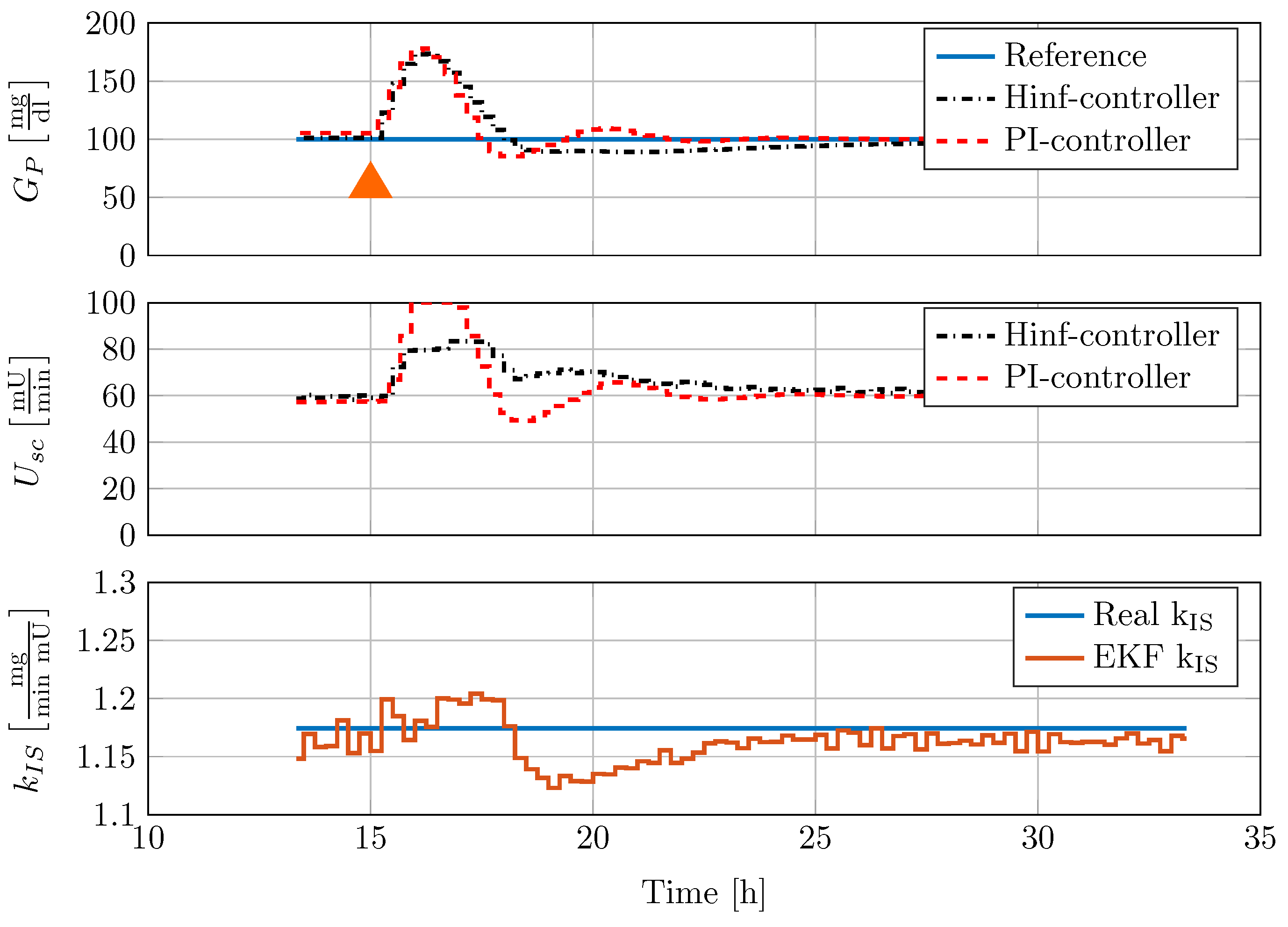
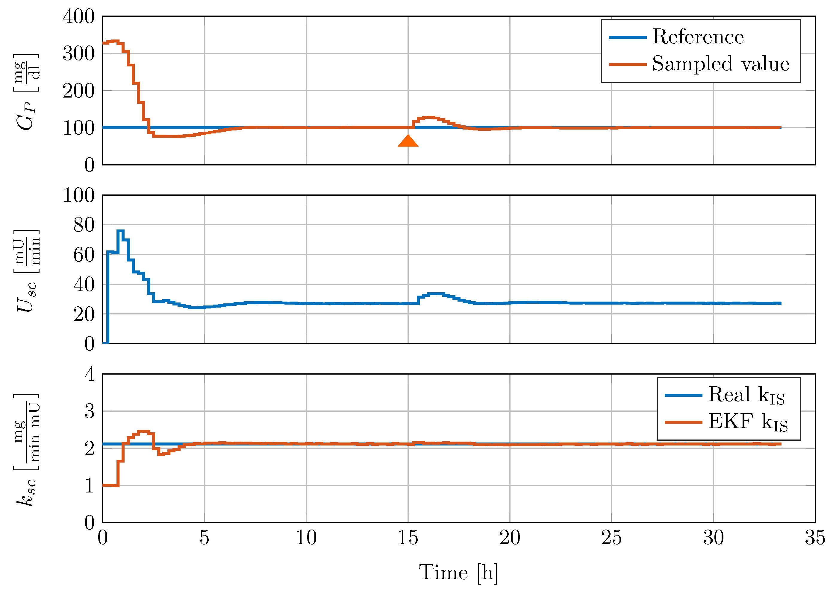
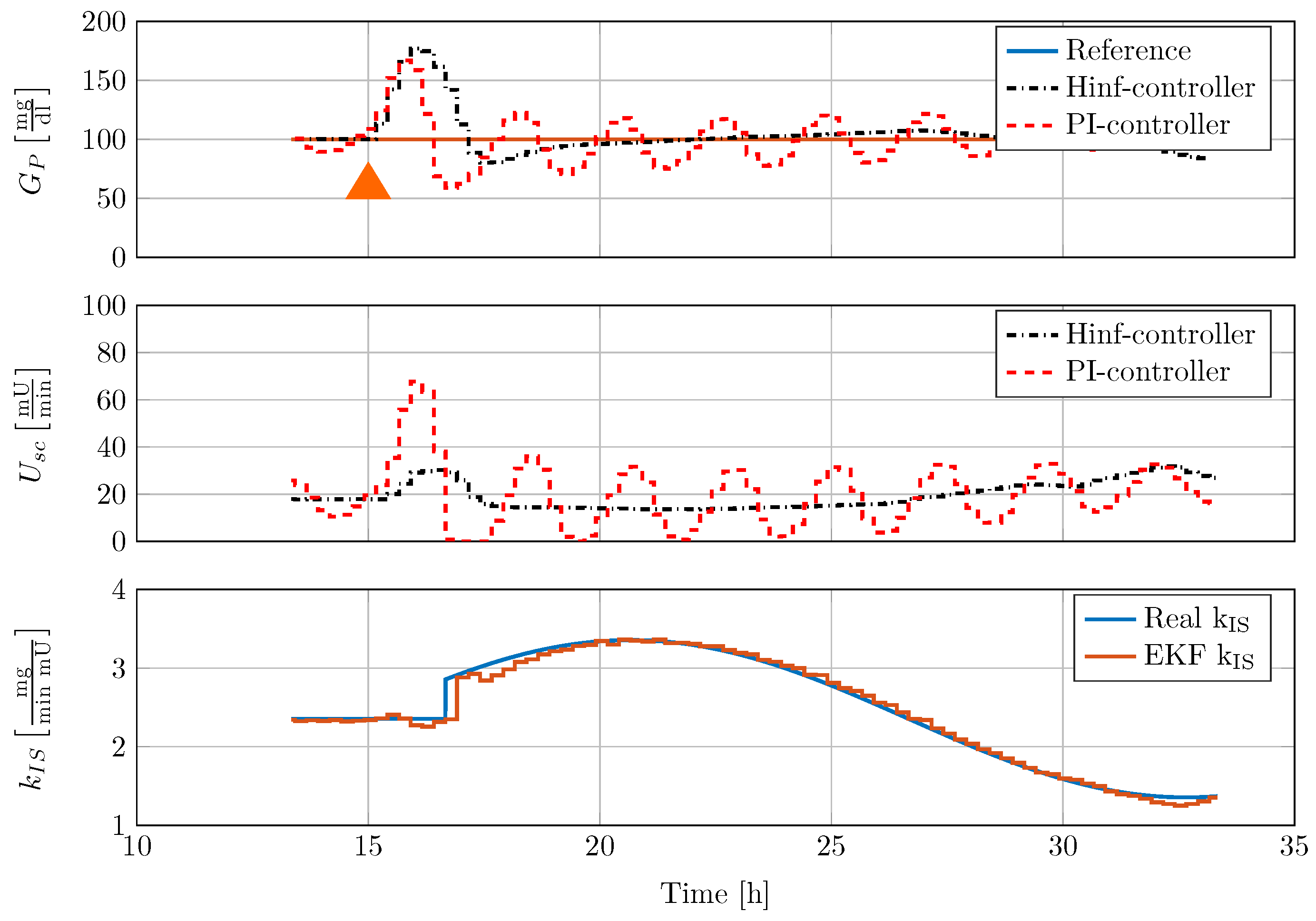
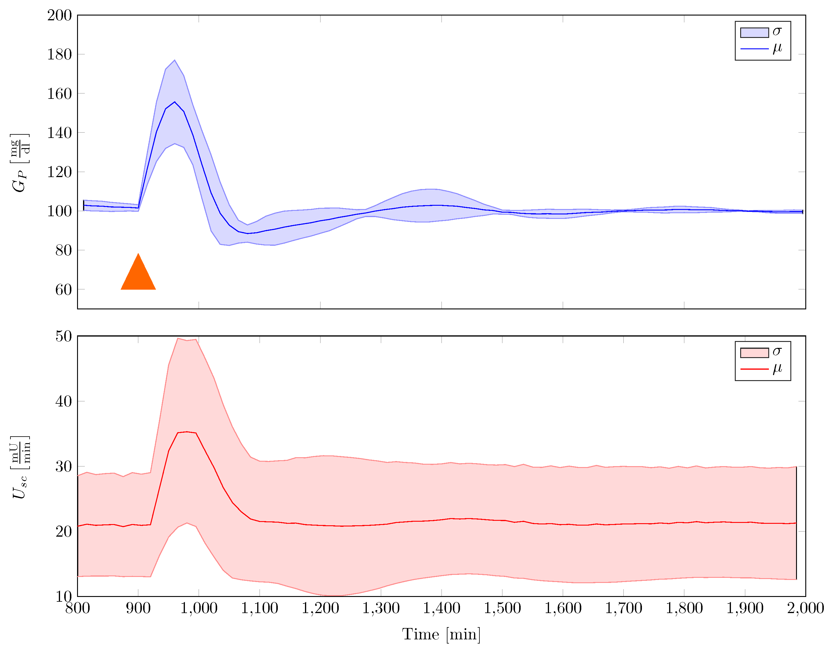
The gain scheduled controller was tested in silico by using the five different full order nonlinear minipig models. Controller implementation was realised with the help of an augmented EKF that estimates insulin sensitivity as a system state. The controller was able to robustly stabilise the family of animal experimental models where additional uncertainty in terms of time-varying insulin sensitivity was included. A comparison with a previously designed classical PI-controller showed superior performance of the new control strategy.

The controller in its current form was implemented without anti-windup protection of the discrete integrator. Moreover, the performance of the gain scheduled controller depends on the accuracy of the insulin sensitivity estimator. As meal uptake and insulin sensitivity cannot be estimated at the same time, due to observability problems, the size of a meal uptake is considered in the estimator by regarding the forward dynamics. Since the subcutaneous application of insulin is considered as uncertain by different authors, a first suitable application of the proposed discrete blood glucose controller seems to be an intensive care unit glucose control scenario. Here, the intravenous-to-intravenous route minimises control input uncertainties, time-delay, and blood glucose sampling time. In its current form, the presented controller design procedure can be readily applied to this scenario, if a suitable model of the process dynamics is available, which can be linearised over the range of blood glucose operating points and insulin sensitivity values. Furthermore, the controller extension with a forward term regarding meal uptake disturbance compensation like, for example, in [12] is possible. The application of the controller in a clinical scenario will be the subject of future work.

References

1. American Diabetes Association. Diagnosis and classification of diabetes mellitus. Diabetes Care 2013, 36, S67–S74. [Google Scholar]
2. Guariguata, L.; Whiting, D.; Hambleton, I.; Beagley, J.; Linnenkamp, U.; Shaw, J. Global estimates of diabetes prevalence for 2013 and projections for 2035. Diabetes Res. Clin. Pract. 2014, 103, 137–149. [Google Scholar] [CrossRef] [PubMed]
3. Melmed, S.; Polonsky, K.S.; Larsen, P.R.; Kronenberg, H.M. Williams Textbook of Endocrinology; Elsevier Health Sciences: Philadelphia, PA, USA, 2015. [Google Scholar]
4. Cobelli, C.; Renard, E.; Kovatchev, B. Artificial pancreas: past, present, future. Diabetes 2011, 60, 2672–2682. [Google Scholar] [CrossRef] [PubMed]
5. Misgeld, B.; Schauer, T.; Simanski, O. Automation of medical systems-Current techniques, limitations and challenges. Biomed. Eng. Biomed. Tech. 2014, 59, 803–806. [Google Scholar]
6. Lunze, K.; Singh, T.; Walter, M.; Brendel, M.D.; Leonhardt, S. Blood glucose control algorithms for type 1 diabetic patients: A methodological review. Biomed. Signal Process. Control 2013, 8, 107–119. [Google Scholar] [CrossRef]
7. Clemens, A. Feedback control dynamics for glucose controlled insulin infusion system. Med. Prog. Technol. 1979, 6, 91–98. [Google Scholar] [PubMed]
8. Hernjak, N.; Doyle, F.J. Glucose control design using nonlinearity assessment techniques. AIChE J. 2005, 51, 544–554. [Google Scholar] [CrossRef]
9. Parker, R.S.; Doyle, F.J.; Ward, J.H.; Peppas, N.A. Robust H glucose control in diabetes using a physiological model. AIChE J. 2000, 46, 2537–2549. [Google Scholar] [CrossRef]
10. Magni, L.; Raimondo, D.M.; Bossi, L.; Dalla Man, C.; De Nicolao, G.; Kovatchev, B.; Cobelli, C. Model Predictive Control of Type 1 Diabetes: An in Silico Trial. J. Diabetes Sci. Technol. 2006, 1, 804–812. [Google Scholar] [CrossRef]
11. Marchetti, G.; Barolo, M.; Jovanovič, L.; Zisser, H.; Seborg, D.E. A feedforward-feedback glucose control strategy for type 1 diabetes mellitus. J. Process Control 2008, 18, 149–162. [Google Scholar] [CrossRef] [PubMed]
12. Garcia-Gabin, W.; Vehi, J.; Bondia, J.; Tarin, C.; Calm, R. Robust sliding mode closed-loop glucose control with meal compensation in type 1 diabetes mellitus. In Proceedings of the 17th World Congress on the International Federation of Automatic Control, Seoul, Korea, 6–11 July 2008; pp. 4240–4245.
13. Walker, D. Robust stabilizability of discrete-time systems with normalized stable factor perturbation. Int. J. Control 1990, 52, 441–455. [Google Scholar] [CrossRef]
14. Sorensen, J.T. A Physiologic Model of Glucose Metabolism in Man and Its Use to Design and Assess Improved Insulin Therapies for Diabetes. Ph.D. Thesis, Massachusetts Institute of Technology, Cambridge, MA, USA, 1985. [Google Scholar]
15. Lunze, K. Blood Glucose Control in Diabetic Göttingen Minipigs; Shaker Verlag: Aachen, Germany, 2014. [Google Scholar]
16. Lunze, K.; Woitok, A.; Walter, M.; Brendel, M.D.; Afify, M.; Tolba, R.; Leonhardt, S. Analysis and modelling of glucose metabolism in diabetic Göttingen Minipigs. Biomed. Signal Process. Control 2014, 13, 132–141. [Google Scholar] [CrossRef]
17. Lunze, K.; Walter, M.; Leonhardt, S. A switching hybrid control method for automatic blood glucose regulation in diabetic Göttingen minipigs. Biomed. Signal Process. Control 2014, 13, 237–246. [Google Scholar] [CrossRef]
18. Hovorka, R.; Canonico, V.; Chassin, L.J.; Haueter, U.; Massi-Benedetti, M.; Federici, M.O.; Pieber, T.R.; Schaller, H.C.; Schaupp, L.; Vering, T.; et al. Nonlinear model predictive control of glucose concentration in subjects with type 1 diabetes. Physiol. Meas. 2004, 25, 905. [Google Scholar] [CrossRef] [PubMed]
19. Laub, A.J.; Heath, M.T.; Paige, C.C.; Ward, R.C. Computation of system balancing transformations and other applications of simultaneous diagonalization algorithms. IEEE Trans. Autom. Control 1987, 32, 115–122. [Google Scholar] [CrossRef]
20. Skogestad, S.; Postlethwaite, I. Multivariable Feedback Control: Analysis and Design; Wiley: New York, NY, USA, 2007; Volume 2. [Google Scholar]
21. Green, M.; Limebeer, D.J. Linear Robust Control; Dover Publications, Inc: Mineola, NY, USA, 2012. [Google Scholar]
22. Strauss, A.; Moskalenko, V.; Tiurbe, C.; Chodnevskaja, I.; Timm, S.; Wiegering, V.A.; Germer, C.T.; Ulrichs, K. Goettingen minipigs (GMP): Comparison of two different models for inducing diabetes. Diabetol. Metab. Syndr. 2012, 4, 7. [Google Scholar] [CrossRef] [PubMed]
23. Misgeld, B.J.; Tenbrock, P.G.; Lunze, K.; Dietrich, J.W.; Leonhardt, S. Estimation of insulin sensitivity in diabetic Göttingen Minipigs. Control Eng. Pract. accepted.
Figure 1. Overview of the artificial pancreas components with reference r ( t ) and disturbance d ( t ) .
Processes 04 00022 g001
Figure 2. Göttingen Minipig model block diagram.
Processes 04 00022 g002
Figure 3. Basic compartment i of the blood glucose model illustrating mass exchange of substance X.
Processes 04 00022 g003
Figure 4. Block diagram of the discrete disturbance rejection controller C ( z ) with hold transfer function H ( s ) and δ-sampler in the feedback branch.
Processes 04 00022 g004
Figure 5. Frequency response of the plant and the disturbance dynamics, comparing full order models G ¯ ( z ) and G ¯ d ( z ) and reduced order models G ^ r ( z and G ^ d r ( z ) .
Processes 04 00022 g005
Figure 6. Frequency response of the compensated open loop (OL) L ( z ) with classical controller and compensated loop L ( z ) with the robust controller.
Processes 04 00022 g006
Figure 7. Comparison of minipig #4 in vivo measurements to in silico results of the identification procedure with individualised Göttingen Minipig data set. The orange triangle indicates a carbohydrate (CHO) uptake of 16 g a the beginning of the experiment. Indicated in the figure is a ±10% confidence interval by the red area.
Processes 04 00022 g007
Figure 8. Block diagram of the discrete disturbance rejection controller C ( z , θ ) implementation with gain scheduling depending on estimated process parameters insulin sensitivity k ^ I S ( k T s ) and blood glucose concentration G ^ p ( k T s ) .
Processes 04 00022 g008
Figure 9. Controller disturbance rejection test with nonlinear minipig model #2. 50 g CHO are given to the minipig at 15 h, indicated by an orange triangle.
Processes 04 00022 g009
Figure 10. Comparison of controller disturbance rejection test with nonlinear minipig model #4. In this figure, 50 mg CHO are given to the minipig at 15 h, indicated by an orange triangle.
Processes 04 00022 g010
Figure 11. Comparison of controller disturbance rejection test with nonlinear minipig model #5 and time-varying insulin sensitivity k I S ( t ) . 50 mg carbohydrates (CHO) are given to the minipig at 15 h, indicated by an orange triangle.
Processes 04 00022 g011
Figure 12. Disturbance rejection statistics with single robust gain-scheduled controller that stabilises the family of Göttingen Minipig model. In this figure, 50 mg CHO are given to the minipig at a time t = 900 min, indicated by an orange triangle (μ—average mean, σ—standard deviation).
Processes 04 00022 g012