A Dynamic Optimization Model for Designing Open-Channel Raceway Ponds for Batch Production of Algal Biomass

Abstract

This work focuses on designing the optimum raceway pond by considering the effects of sunlight availability, temperature fluctuations, and harvest time on algae growth, and introduces a dynamic programing model to do so. Culture properties such as biomass productivity, growth rate, and concentration, and physical properties, such as average velocity, pond temperature, and rate of evaporation, were estimated daily depending on the dynamic behavior of solar zenith angle, diurnal pattern of solar irradiance, and temperature fluctuations at the location. Case studies consider two algae species (Phaeodactylum. tricornutum and Isochrysis. galbana) and four locations (Tulsa, USA; Hyderabad, India; Cape Town, South Africa; and Rio de Janeiro, Brazil). They investigate the influences of the type of algae strain and geographical location on algae biomass production costs. From our case studies, the combination of I. galbana species grown in Hyderabad, India, with a raceway pond geometry of 30 cm channel depth, about a meter channel width, and 300 m in length, and a harvest interval of every six days yielded the minimum algal biomass production costs. The results of the sensitivity analysis reveal that smaller channel depths and longer ponds (within the ranges considered) are recommended to minimize the net present cost of algae biomass production.

1. Introduction

Large-scale production of micro-algal biomass is achieved by open pond cultivation technologies [1]. Open pond cultivation technologies have been known since 1950s. They can be classified as circular ponds, unmixed ponds, inclined ponds, and raceway ponds, depending on their design and operation [2]. The most preferable among them for algae cultivation are raceway ponds [3]. They are single or multiple closed-loop oval-shaped recirculation channels with paddle wheel that enable circulation and prevent sedimentation. The principal advantages of raceway pond cultivation technology are small capital investment, use of free solar energy [2], easy maintenance, and lower energy requirements [4]. The idea of cultivating algae for the purpose of biofuels production was first investigated by Oswald W. J. in 1970s. Later, in 1978, the U.S. Department of Energy’s Aquatic Species Program attempted to identify the algal species and conditions that would generate a cost-effective algae biofuels production [5]. This eighteen-year program explored open ponds and yielded a collection of high oil producing species.

There is a significant body of literature that studies the cultural properties of algal biomass for a given outdoor raceway pond or focuses on designing new outdoor pond configurations. In 1979, a theoretical framework was developed by Goldman for continuous culturing of algal biomass to predict the biomass productivity as a function of sunlight and temperature in open raceways [6]. The model also took into account the effects of culture depth and nutrients on light intensity. The upper limit on biomass yield was determined to be 30–40 dry·g·m⁻²·day⁻¹. Hill and Lincoln developed a mathematical model for continuous flow mass culture of microalgae in multi rectangular open channels. The model predicted algal production, dissolved oxygen, pH, and concentrations of nutrients [7]. Grobbelaar et al. developed a deterministic mathematical model to describe the production of the green microalgae Scenedesmus. obliquus (S. obliquus) and Coelastrum. sphaericum (C. sphaericum) in outdoor raceways [8]. Assuming that CO₂ and other nutrients were supplied in excess during cultivation, the dynamic model incorporated sixteen months of irradiance and temperature measurements to evaluate the productivity. The productivity varied between 1.7 and 16.92 g·m⁻²·day⁻¹. Sukenik et al. developed a deterministic simulation model to estimate productivity of the marine algae Isochrysis. Galbana (I. galbana) in an outdoor raceway pond [9]. The effects of pond depth and chlorophyll concentration on production rate were evaluated in various seasons. The model predicted an annual average productivity of 9.7 g of carbon uptake per square meter per day (gC·m⁻²·day⁻¹). A new regulatory model was developed by Geider et al. [10] to describe the acclimation of phytoplankton growth rate to irradiance, temperature and nutrient availability. The model used Poisson function to model photosynthesis, Arrhenius function to model temperature and Michaelis-Menten kinetics to model nutrient uptake. James et al. [11] simulated hydrodynamics coupled with growth kinetics of Phaeodactylum. tricornutum (P. tricornutum) in open-channel raceways using modified versions of Environmental Fluid Dynamics Codes (EFDC) [12] and U.S. Army Corp of Engineers’ water quality code (CE-QUAL) [13]. System parameters such as flow velocity and raceway depth were varied to improve growth rate. Their results show that the depth of the pond should vary in response to the atmospheric temperature to maximize algae yield. They also reported that increasing the flow rate above 6.25 L/s does not further improve the algae growth rate.

Ketheesan et al. developed a new airlift-driven raceway configuration, that is paddle wheel free, for energy-efficient algal cultivation [14]. Harvesting was performed after 14 days when culture reached the end of linear growth phase. Sompech et al. used computational fluid dynamics to model the energy consumption, the extent and location of dead zones in various geometric configurations of raceway ponds at various flow velocities [15]. They concluded that the standard configuration with baffles on each end are relatively inexpensive and prevented the formation of dead zones. Chiaramonti et al. designed an innovative raceway pond and compared its performance with conventional raceway pond [16]. The innovative raceway pond was shallower and paddle wheel was replaced by centrifugal pump. They investigated the energy consumption and concluded that the new design saved 50% energy over an area of 500 m². Talent et al. [17] developed a protocol for harvesting microalgae massive cultures from open ponds. According to them, a minimum of 10% of the pond volume per day should be harvested and replaced with new feedstock water.

Many studies focus on predicting the culture properties such as productivity, growth rate, and biomass concentration depending on the sunlight and temperature fluctuations at a given facility under known pond configurations. Other studies include varying the raceway pond geometry to understand the physical parameters such as average velocity, evaporation rate, energy consumption and their influence on operating costs. The optimum pond geometry depends on the growth characteristics such as biomass concentration, growth rate, and productivity of the algae species which are affected by sunlight availability and temperature fluctuations at a location. There is a gap in literature of a model that relates all three: pond geometry, location and type of algae species. The key contribution of this paper is the development of a dynamic programming formulation that considers algae strain characteristics, diurnal pattern of solar irradiance, temperature fluctuations, and harvesting intervals to yield the optimum design configuration of an outdoor raceway pond. The model defines optimum design as the one that minimizes total production cost for a plant life of 10 years, including both capital and operating costs. Our model also captures the dynamics of biomass concentration, average light inside the pond, growth rate, production, and radiation entering and leaving the pond.

2. Problem Statement

Given an algae species, a geographical location to grow algae, and algal biomass demand, the goal is to obtain the optimum raceway pond geometry considering the effect of physical parameters such as temperature fluctuations in the growth media, diurnal pattern of sunlight, harvest schedule, light limitation, and evaporation losses. Here, the optimum design is the one that yields the minimum net present cost for biomass production with a plant life of 10 years. The net present cost is a combination of both capital costs and operating costs. Capital costs include site preparation, grading, compaction, pond levees, paddle wheel, CO₂ diffusers, harvesting, flocculation, centrifugation, water and nutrient supply system, waste treatment system, buildings and structures, electrical supply and distribution, instrumentation and machinery, land, and engineering and contingency costs. Operating costs include electricity, water, nutrients, flocculants, waste disposal, maintenance and repairs, operating supplies, depreciation, taxes and insurance, financing, labor and overhead costs, and general expenses.

3. Algal Production Model for Raceway Ponds

This section explains the changes in culture properties of the algae species and their dependencies on the geometry of the raceway pond and weather conditions at the location.

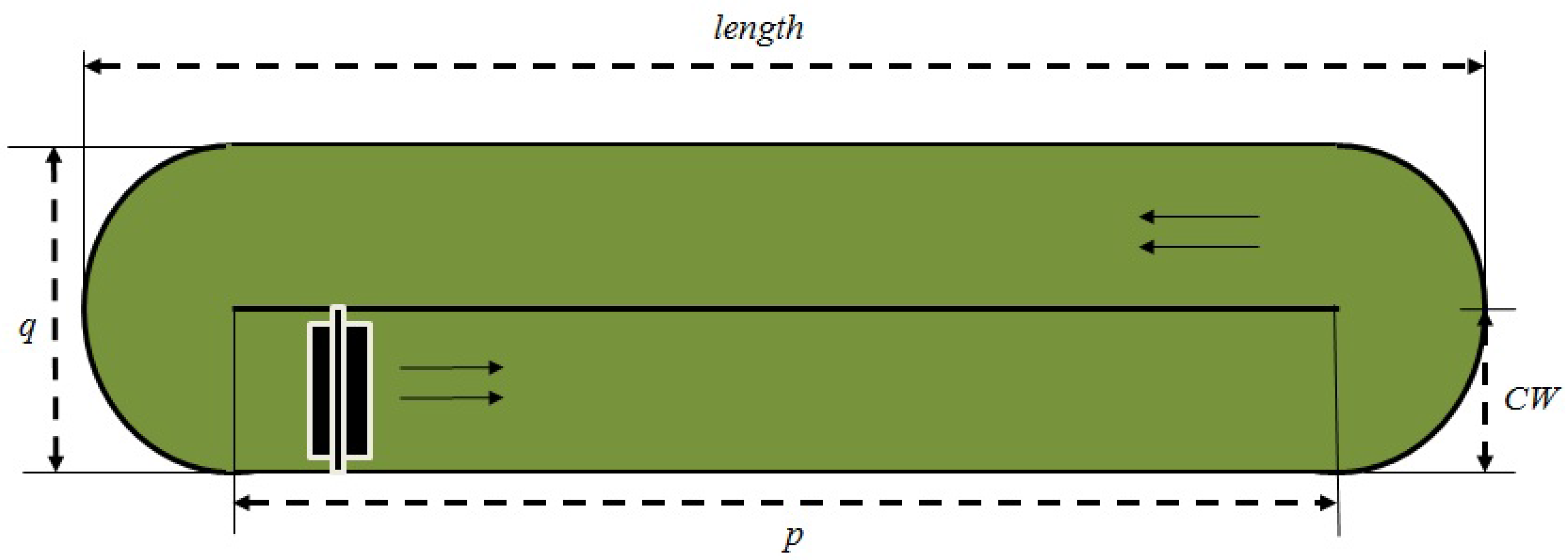
Algae growth: Figure 1 shows the aerial view of the raceway pond and its geometry.

The pond is considered to be perfectly mixed and of uniform concentration. However, the concentration changes with time due to algae growth. Equation (1) explains the dynamic changes occurring in biomass concentration with the production of dry algae in a given pond volume V (assuming constant density). In the pond, with time as algae cells begin to multiply, biomass concentration rises. In our model, we considered seeding the pond just before sunrise, i.e., biomass concentration, has been initialized to certain value just before sunrise after harvest.

$$V\frac{dBC(t)}{dt}=\frac{d{X}_{DA}(t)}{dt}$$

(1)

here, V (m³) is the volume of the raceway pond and BC (g·m⁻³) and X_DA (g) represent the biomass concentration and the amount of dry algae in the pond at any given time.

The amount of sunlight reaching the algae cells inside the pond varies depending on the accumulation of biomass, the culture’s light absorption coefficient, and the depth of the pond. During the cultivation of algae in outdoor raceway ponds, light intensity is attenuated because of gradual increase in the concentration of biomass [18] and due to uneven absorption of light by algae cells. The algae cells closer to light source receive higher irradiance than cells further away. Grima et al. proposed an empirical relationship between light attenuation and biomass concentration, and verified its accuracy for several types of freshwater microalga, P. tricornutum [19]. The model was later validated for different algae species and photobioreactor orientations in literature [20]. The model first, estimates the average solar irradiance, I_avg(t) (µE·m⁻²·s⁻¹), experienced by a single cell moving inside the culture medium (via Equation (2)) based on the position of the sun relative to the pond and Beer-Lambert relationship [21].

$$I_{avg}(t)=\frac{I_o(t)}{Ka\cdot BC(t)\cdot C{D}_{eq}(t)}\left[1-e^{-\left(Ka\cdot BC(t)\cdot C{D}_{eq}(t)\right)}\right]$$

(2)

In Equation (2), Ka is light absorption coefficient and varies with algae species. I_o(t) (µE·m⁻²·s⁻¹) is the incident light on the surface which is a function of daily maximum and minimum temperatures as explained by Hargreaves [22]. It is shown via Equation (24) of the Supplementary Materials provided with this manuscript. CD_eq(t) is the length of light path from the surface to any point inside the pond. The length of light path depends on the depth of the pond, CD (m), and the position of the sun relative to the earth’s surface called solar zenith angle as shown in Equation (3). The greater the pond depth, the longer is the length of the light path. The lower the sun’s position from the Earth’s surface, during sunrise and sunset, the longer is the length of the light path in the pond. However, when the sun’s position is high in the sky, the length of the light path is shorter.

$$C{D}_{eq}(t)=\frac{CD}{\cos \theta (t)}$$

(3)

Growth rate of algae cells depend on their light extinction coefficient, I_k (μE·m⁻²·s⁻¹), and the availability of light inside the pond, I_avg(t) as shown in Equation (4). The equation does not take into account photoinhibition. Although it is well documented, it has often been disregarded. Studies suggest that growth models that express µ in terms of the average irradiance raised to some power greater than unity better fit experimental observations [21,23]. Equation (4) is a light-limited growth equation which was developed and tested by Grima, Camacho, Pérez, Sevilla, Fernández, and Gómez [19]. Based on the study, material balance performed in a chemostat where specific growth rate is expressed as a function of irradiance, it was observed that the algae growth rate predictions of this model exhibit a good agreement with the measured ones. It models the effect of light attenuation on the observed algae growth rate in the cultivation unit. It defines a hyperbolic relationship between the specific growth rate of algae and average solar irradiance inside the culture.

$$\mu (t)={\mu }_{\max }(t)\left[\frac{I_{avg}^n(t)}{I_k^n+I_{avg}^n(t)}\right]$$

(4)

here, n is an exponent that describes the abruptness of the transition from weakly-illuminated to strongly-illuminated regions and is obtained from non-linear regression analysis on light intensity as a function of biomass concentration [19].

The maximum specific growth rates, μ_max, (day⁻¹) of algae species depend strongly on the temperature of the pond and the species itself [24]. Several models describe the influence of temperature on growth rate of algae, we have chosen the model presented in [25] where eight species of marine phytoplankton were grown at different temperatures ranging from 10 to 25 °C. They experimentally modeled the general response of growth rate to temperature as ${\mathsf{\mu }}_{max}=\mathsf{\alpha }.exp\left(\mathsf{\beta }.T\right)$ where α and β are species dependent constants and T is temperature of medium. In our work, we have used their data to model the growth response of the selected species. We used the same relationship in our model via Equation (5).

$${\mu }_{\max }(t)=\alpha \exp (\beta T_{pond}(t))$$

(5)

where T_pond is temperature of the pond. The species specific constants α and β are taken from our previous findings [26]. The experimental data modeled the response of growth rates of eight species of marine phytoplankton to changes in temperature under continuous light [27].

Growth rate, biomass concentration, and algae cells in the pond are interrelated. The biomass concentration and the specific growth rate determine the rate of change of algal biomass in the pond. This relation is shown via Equation (6). As the biomass concentration and growth rate increase from sunrise to further during the day, the algae cells multiply. However, as concentration further increases, the growth rate begins to decline due to mutual shading, thus effecting the production of algae cells.

$$BC(t)\mu (t)=\frac{1}{V}\frac{d{X}_{DA}(t)}{dt}$$

(6)

Temperature of the pond is essential for proper design and optimal operation of algal ponds. Based on the pond temperature, algae could either exhibit optimal growth characteristics or could perish above a certain threshold temperature. In this work, pond temperature is calculated using the temperature model that is “universally applicable” for shallow ponds containing opaque water body [28]. According to Béchet, Q., et al., the model was tested against experimental data that has been collected for a period of one year from a wastewater treatment high-rate algal pond and was validated with a “high degree of accuracy” [28]. The model is shown explicitly via Equations (7) through (17). Here, the pond temperature, T_pond(t) (K), is calculated via an overall energy balance around the pond (Equation (17)). According to [28], conduction was of low importance in the total heat balance for shallow algae ponds. Thus conductive heat flux is neglected for this model since we assume no heat transfer between the pond bottom and the soil beneath. We also ignored the changes in pond temperature caused due to rainfall, and hence, removed the rain heat flux term from the model. Therefore, temperature of the outdoor pond is determined by six heat fluxes: (1) Heat flux due to pond radiation; (2) heat flux due to solar radiation; (3) heat flux due to air radiation; (4) Evaporation; (5) Convection; and (6) Inflow heat flux.

(1) Heat flux due to pond radiation: Radiation from the pond’s surface to the atmosphere Q_p(t) is estimated by Stefan-Boltzmann’s fourth power law as shown in Equation (7) [28]. Since heat transfer takes place from pond surface to the atmosphere, this heat flux is negative. The higher the radiation from the pond, the higher heat transfer from pond to the atmosphere becomes, which lead to lower pond temperature.

$$Q_p(t)=-{\epsilon }_w\sigma T_{pond}^4(t)SA$$

(7)

where ε_w = 0.97 represents the emissivity of water [29], σ = 5.67 × 10⁻⁸ represents Stefan-Boltzmann constant (W·m⁻²·K⁻⁴) and SA is the surface area of the pond (m²). (2) Heat flux due to solar radiation: Radiation received by the pond from the sun Q_s(t) is calculated from incident irradiance on the surface in Equation (8) [28]. The higher the radiation from the sun to the pond, the higher would be the temperature of the pond.

$$Q_s(t)=\left(1-f_a\right)I_o(t)SA$$

(8)

where f_a is the fraction of sunlight converted by algae into chemical energy during photosynthesis. It is assumed to be constant and equal to 2.5%. (3) Heat flux due to air radiation: Radiation from air, Q_a(t), is given by Stefan-Boltzmann’s fourth power law as shown in Equation (9) [28]. T_surr(t) (K) is calculated by the method outlined by Woodhead [30]. The higher the radiation from the air to the pond, the higher would be the pond temperature.

$$Q_a(t)={\epsilon }_w{\epsilon }_a\sigma T_{surr}^4(t)SA$$

(9)

where ε_a = 0.8 represents the emissivity of air. (4) Evaporation: Evaporative heat transfer, Q_ev(t), is related to rate of evaporation, me(t) (kg·m⁻²·s⁻¹), and it is expressed in Equation (10) [28].

$$Q_{ev}(t)=-me(t)L_{w}SA$$

(10)

where L_w = 2.45 × 10⁶ J·kg⁻¹ represents the latent heat of water. Theoretically, applying Buckingham theorem to evaporation at the pond surface yields three dimensionless numbers namely, the Sherwood number Sh_L, the Schmidt number Sch_L, and the Reynolds number Re_L. The rate of evaporation is shown to be dependent on the three dimensionless numbers [31]. For mass transfer in a horizontal surface, the three dimensionless groups are correlated as follows:

$$S{h}_L=0.035{\left(R{e}_L\right)}^{0.8}{\left(Sc{h}_L\right)}^{1/3}$$

(11)

where Sherwood number:

$$S{h}_L=\frac{K\left(t\right)\cdot D_h}{D_{w,a}}$$

(11A)

Schmidt number:

$$Sc{h}_L=\frac{{\vartheta }_a}{D_{w,a}}$$

(11B)

Reynolds number:

$$R{e}_L=\frac{D_h\cdot WV(t)}{{\vartheta }_a}$$

(11C)

where K is the mass transfer coefficient (m·s⁻¹) determined via Equation (11), D_h is the hydraulic diameter of the pond (m), D_w,a = 2.4 × 10⁵ m²·s⁻¹ represents the mass diffusion coefficient of water vapor in air, ϑ_a = 1.5 × 10⁵ m²·s⁻¹ denotes the air kinematic viscosity, and WV(t) represents the wind velocity (m·s⁻¹). Equation (11) has been derived with an assumption that wind is constant with respect to height. The rate of evaporation is calculated by Equation (12).

$$me(t)=K\left(t\right)\left[\frac{P{}_w\left(t\right)}{T_{pond}(t)}-\frac{RH(t)P_a\left(t\right)}{T_{surr}(t)}\right]\frac{M{W}_{H_{2}O}}{R}$$

(12)

where MW_H2O is the molecular weight of water (kg·mole⁻¹), R = 8.314 Pa·m³ mol⁻¹·K⁻¹ is the ideal gas constant, and RH(t) represents the relative humidity of the air over the pond surface. Relative humidity is important with regard to both evaporation losses and pond cooling. When humidity is low, high rates of evaporation occur, particularly during windy periods. When humidity is high and there is little or no wind, and when sunlight is abundant, the water in shallow cultures may heat up. In Equation (12), P_a and P_w are saturated vapor pressures (Pa) at T_surr and T_pond, respectively, and can be determined using Equation (13) [32].

$$P_i\left(t\right)=3385.5e^{-\left[-8.0929+0.97608{\left(T_i\left(t\right)+42.607-273.15\right)}^{0.5}\right]}$$

(13)

(5) Convection: Convective heat transfer, Q_cv(t), is expressed similar to evaporative heat transfer as heat transfer and mass transfer obey the same laws. Applying Buckingham theorem to convection at the pond surface yields three dimensionless numbers namely, the Nusselt number, the Prandtl number, and the Reynolds number. Convection coefficient is calculated using the correlation between the three dimensionless numbers (Equation (14)) [31].

$$N{u}_L=0.035{\left(R{e}_L\right)}^{0.8}{\left(Pr\right)}^{1/3}$$

(14)

where Nusselt number:

$$N{u}_L=\frac{h_{cv}(t)\cdot D_h}{{\lambda }_a}$$

(14A)

Prandtl number:

$$Pr=\frac{{\vartheta }_a}{{\alpha }_a}$$

(14B)

Reynolds number:

$$R{e}_L=\frac{D_h\cdot WV(t)}{{\vartheta }_a}$$

(14C)

where h_cv(t) (W·m⁻²·K⁻¹) is the convection coefficient, λ_a = 2.6 × 10² W·m⁻¹·K⁻¹ represents air thermal conductivity, and α_a = 2.2 × 10⁵ m²·s⁻¹ represents air thermal diffusivity. The convective heat flux Q_cv(t) is given by Equation (15).

$$Q{}_{cv}(t)=h_{cv}(t)\left(T_{surr}(t)-T_{pond}(t)\right)SA$$

(15)

(6) Inflow heat flux: The heat transfer associated with the water inflow Q_i(t) can be expressed as a steady flow thermal energy equation shown in Equation (16). Water is added to compensate for evaporation from the pond surface, and it is assumed to be at the surrounding temperature T_surr(t) when added to the pond.

$$Q_i(t)=\left(me(t)\cdot SA\right)Cp\left(T_{surr}(t)-T_{pond}(t)\right)$$

(16)

where the first set of parenthesis indicates mass flow rate of incoming water. It is the product of rate of evaporation and surface area of the pond. Cp represents the specific heat capacity of the pond water (J·g⁻¹·K⁻¹). The overall energy balance for the pond is given in Equation (17).

$$\dot{m}(t)Cp\frac{\partial T_{pond}(t)}{\partial t}=Q_p(t)+Q_s(t)+Q_a(t)+Q_{ev}(t)+Q_{cv}(t)+Q_i(t)$$

(17)

In Equation (17), Q_p(t) is the rate of heat flow from the pond surface (W), Q_s(t) is the rate of heat flow from sun to the pond (W), Q_a(t) is the rate of heat flow from air to the pond (W), Q_ev(t) is the rate of heat flow by evaporation (W), Q_cv(t) is the rate of heat flow by convection at the surface of the pond (W), and Q_i(t) is the rate of heat flow associated with water inflow (W). The mass flow rate, $\dot{m}$(t), can be calculated via Equation (18) using the concepts of fluid dynamics where mass flow rate is density times volumetric flow rate.

$$\dot{m}(t)=\rho \cdot U_{avg}(t)\cdot CW\cdot CD$$

(18)

where ρ is the density of water, U_avg(t) is the average daily velocity of the pond, CW is the channel width, and CD is the channel depth.

The proposed model assumes no cloud coverage, and hence, it ignores the effects of cloud cover on biomass growth rate and productivity. The model also assumes the usage of atmospheric carbon dioxide at no additional cost. Nutrients, such as nitrogen and phosphorus, are assumed to be supplied, as needed, in their appropriate forms for algal growth in the growth medium. The pond is assumed to be completely mixed, and all physical properties are assumed to be that of water under standard conditions.

4. Dynamic Model

The objective of the optimization model is to find the raceway pond geometry that best suits the chosen location to grow the desired algae species. The objective function, to be minimized, considers the overall production costs involved. A complete listing of the subscripts, parameters, variables, and constraints of the program is given below.

4.1. Subscripts

The indices used in the model are: (1) s: Microalgae species; (2) l: Location; (3) c: Component, including algae biomass, DA (dry algae biomass), WIA (water present in algae biomass), WW (waste water); (4) y: Year; (5) d: day; and (6) hd: Harvest day.

4.2. Parameters

Parameters used in the model are given as follows: (1) efficiency of paddle wheel (η_PW); (2) empirical constant for interior regions (EmpA) and coastal regions (EmpB) used for calculating incident irradiance at a location; (3) solar constant (μE·m⁻²·s⁻¹) (Sc); (4) initial biomass concentration (g·m⁻³) at seeding of the pond (BCini); (5) algae biomass (g) demand (demand); (6) number of days between harvests is harvest period (harvP); (7) number of harvest periods in a month is harvest cycle (harvC); and (8) density (g·m⁻³) of water (ρ).

Different algae strains have different lipid contents, nutrient requirements, and tolerance levels for temperatures. In this work, the microalgae species selected for outdoor cultivation have three parameters: (1) percentage of dry algae present in microalgae (%) of species s (%_s); (2) light absorption coefficient (m²·g⁻¹) of biomass (Ka_s); and (3) a species dependent constant (μE·m⁻²·s⁻¹) used in the calculation of growth rates (I_k,s). Similarly, the relevant parameters for a geographical location are: (1) latitude of location l (latitude_l); (2) longitude of location l (longitude_l); (3) time zone of location l (TZ_l); (4) average maximum and minimum temperatures (°C) of the day (T_maxl,d and T_minl,d); (5) surrounding temperature (°C) (T_surrl,d(t)); (6) total capital cost coefficient ($·m⁻²) at location l (TCI_l); (7) total operating cost coefficient ($·m⁻²) at location l (TPC_l); (8) electricity costs ($·kWh⁻¹) at location l (ElCost_l); (9) water costs ($·m⁻³) at location l (WtCost_l); (10) availability of sunlight at location l (μE·m⁻²·s⁻¹) (I_ol (t)); (11) relative humidity (%) for location l (RH_l,d(t)); (12) wind velocity (m·s⁻¹) at location l (WV_l,d(t)); (13) sunrise time for location l (sunrise_l,d); (14) sunset time for location l (sunset_l,d); and (15) zenith angle for location l (θ_l,d(t)).

4.3. Decision Variables

Depending on their function, variables used in designing the raceway pond can be categorized into three types: culture properties, physical properties and design properties.

Culture properties are: (1) biomass concentration (g·m⁻³) (BC(t)); (2) biomass concentration (g·m⁻³) on harvest day hd (BCharv_hd,(t=sunset_l)); (3) biomass specific growth rate (h⁻¹) (µ(t)); (4) biomass maximum specific growth rate (h⁻¹) (µ_max(t)); (5) biomass volumetric productivity (g·m⁻³·day⁻¹) (PrV).

Physical properties are defined as: (1) average velocity (m·s⁻¹) of the pond (U_avg(t)); (2) average irradiance (μE·m⁻²·s⁻¹) inside the pond (I_avg(t)); (3) length (m) of light path from the surface to any point in the pond (CD_eq(t)); (4) mass (g) of component c (X_c(t)); and (5) accumulation (g) of component c until harvest day hd (Xharv_c,hd(t=sunset_l)) (g); (6) annual production (g) of component c (D_c,y); (7) mass (g) of products accumulated (m(t)); (8) Areal productivity (g·m⁻²·day⁻¹) (PrA); (9) Reynolds number of flowing stream (Re_d); (10) pond temperature (°C) (T_pond(t)); (11) heat transfer (W) due to pond radiation (Q_r(t)); (12) heat transfer (W) due to solar radiation (Q_s(t)); (13) heat transfer (W) due to air radiation (Q_a(t)); (14) heat transfer (W) due to evaporation (Q_ev(t)); (15) heat transfer (W) due to convection (Q_cv(t)); (16) heat transfer (W) due to inflow water (Q_i(t)); (17) head loss (m) due to friction (h_F); (18) kinetic head loss (m) (h_K); (19) total head loss (m) (h_T); (20) power needed to drive the paddle wheel (W) (PP(t)); (21) annual energy (kWh) requirements of paddle wheel (kW) (EPP); (22) annual water (m⁻³) requirements (Awater); (23) power needed to supply the water lost during harvesting, evaporation, and recycling (W) (PW(t)); (24) annual energy (kWh) requirements of pumping lost water (kW) (EPW); (25) Industrial water (m³) added into the pond (Indwater).

Design properties are defined with the following variables: (1) pond depth (m) (CD); (2) channel width (m) (CW); (3) pond length (m) (length); (4) pond width (m) (q); (5) channel length (m) (p); (6) hydraulic diameter (m) (D_h); (7) pond volume (m³) (V); and (8) pond surface area (m²) (SA).

4.4. The Model

The objective is to fulfill the biomass demand at a minimum net present cost, Z, for a raceway pond with a plant-life of 10 years. The objective function and constraints are as follows:

$$Z=Z_{Cap-cost}+{\displaystyle \sum _{p=0}^{10}\frac{1}{{\left(1+MARR\right)}^p}}\left[Z_{Electric-mixing}+Z_{Electric-pumping}+Z_{Water}+Z_{Product-cost}\right]$$

(19)

where

$$Z_{Cap-cost}=TC{I}_l\cdot SA$$

(20)

$$Z_{Electric-mixing}=ElCos{t}_l\cdot EPP$$

(21)

$$Z_{Electric-pumping}=ElCos{t}_l\cdot EPW$$

(22)

$$Z_{Water}=WtCos{t}_l\cdot Indwater$$

(23)

$$Z_{Product-cost}=TP{C}_l\cdot SA$$

(24)

subject to:

$$D_{algaebiomass,y}\ge demand\forall y$$

(25)

$$D_{algaebiomass,y}=D_{DA,y}+D_{WIA,y}\forall y$$

(26)

$${\displaystyle \underset{t}{\int }{X}_{WIA}(t)}dt=D_{WIA,y}$$

(27)

$${\displaystyle \underset{t}{\int }{X}_{DA}(t)}dt=D_{DA,y}$$

(28)

$$X_{WIA}(t)=\frac{100X_{DA}(t)}{{\%}_s}-X_{DA}(t)$$

(29)

$$X_{WW}(t)=\left[\frac{X_{DA}(t)}{BC(t)}\right]\rho$$

(30)

$$m(t)=X_{DA}(t)+X_{WIA}(t)+X_{WW}(t)$$

(31)

$$q=2CW$$

(32)

$$length=p+q$$

(33)

$$SA=\frac{\pi q^2}{4}+pq$$

(34)

$$V=SA\cdot CD$$

(35)

$$PrV=\frac{D_{DA,y}}{V\cdot 360}$$

(36)

$$PrA=\frac{PrV\cdot V}{SA}$$

(37)

$$h_L(t)=\frac{U_{avg}^2(t)\cdot R{C}^2\cdot length}{D_h^{\frac{4}{3}}}$$

(38)

$$h_K(t)=\frac{K\cdot U_{avg}^2(t)}{2g}$$

(39)

$$h_T(t)=h_L(t)+2h_K(t)$$

(40)

$$PP(t)=\frac{\dot{m}(t)\cdot g\cdot h_T(t)}{{\eta }_{PW}}$$

(41)

$$PW(t)=\frac{2\left(me(t)\cdot SA\right)\cdot \mu \cdot length\cdot {\left(2CD+CW\right)}^2\cdot U_{avg}(t)}{\rho \cdot C{D}^2\cdot C{W}^2}$$

(42)

$$EPP={\displaystyle \underset{t}{\int }PP(t)}dt$$

(43)

$$EPW={\displaystyle \underset{t}{\int }PW(t)dt}$$

(44)

$$CD\ge 30cm$$

(45)

$$length\le 300m$$

(46)

$$\frac{p}{q}\ge 10$$

(47)

$$PrA\le 60g/m^2/day$$

(48)

$$0.1m/s\le U_{avg}(t)\le 0.3m/s$$

(49)

$$BC(t)\le 10000g/m^3$$

(50)

$$BC(t)-BC(t-1)=\frac{X_{DA}(t)-X_{DA}(t-1)}{V}$$

(51)

$$BC(t)\cdot \mu (t)=\frac{X_{DA}(t)-X_{DA}(t-1)}{V}$$

(52)

The objective function, Equation (19), is the net present cost. It includes capital costs: Z_Cap-cost and operating costs: Z_{Electric-mixing}, Z_{Electric-pumping}, Z_Water, and Z_Product-cost. The Minimum Acceptable Rate of Return (MARR) is 15%. Equation (20) assumes that the capital cost changes linearly with the pond surface area. Equations (21) and (22) calculate the cost of electricity required for mixing using paddle wheel and cost of electricity required for pumping additional water that is lost during evaporation. Equation (23) estimates the cost of water. Equation (24) calculates the total production cost. The estimation of cost coefficients for capital costs (TCI_l) and operating costs (TPI_l) are detailed in Section 6.1.

The first constraint, Equation (25), makes sure that the specified annual algae biomass demand is met. The second constraint, Equation (26), shows that the total annual production of wet algae biomass is the sum of annual production of dry algae biomass and water in algae. Equations (27) and (28) show that sum of water in algae and dry algae produced at different times in a year is equal to their annual productions. Equation (29) calculates the hourly production of WIA (water present in algae), given the percentage of dry algae in wet algae biomass for species s. The next constraint, Equation (30), shows the dependence of excess waste water on biomass concentration. If the biomass concentration is high, waste water production is low and vice versa. Also, the higher the biomass concentration, the higher is the dry algae present inside the pond. Total mass (DA, WIA, and WW) in the pond at any time is computed via Equation (31).

Equations (32) through (35) represent pond related geometric constraints. Ponds should have minimum number of bends to keep the energy required for recirculation to a minimum [33]. Hence, this work focuses on the design of single channel raceway pond where the relationship between pond width and channel width is given in Equation (32). Pond length is the sum of channel length and pond width as shown in Equation (33). Surface area occupied by the pond is computed from Equation (34). To avoid the flow disturbance caused by the bends of the raceway pond, the ratio of pond length to width should be 10 or greater [33], and this requirement is enforced via Equation (47). Equation (35) calculates the volume of the raceway pond.

Equation (36) calculates the average daily volumetric productivity of microalgae on dry weight basis. Areal productivity is calculated as shown in Equation (37). Equations (45) and (46) are the bound constraints on pond depth and length. Pond depth should always be above an acceptable limit which may otherwise lead to pond evaporation and biomass solidifying issues. In our work, sensitivity analysis was performed on the lower bound of depth to see its impact on the dynamic changes of biomass concentration. Pond length is constrained to keep the head loss due to friction lower. The acceptable bounds on pond depth and length are taken from literature [34]. Equation (48) specifies an upper bound on the average daily areal productivity of microalgae to be 60 g·m⁻²·day⁻¹ [35]. The cost coefficients in the objective function, TCI_l and TPC_l, were taken assuming the average daily areal productivity of 60 g·m⁻²·day⁻¹.

Equations (38) (Manning’s equation) and (39) calculate frictional and kinetic head losses [36]. Total head loss is calculated in Equation (40) [36]. Power required for maintaining flow in the raceway, i.e., power of paddlewheel is given by Equation (41) [36]. Power required for pumping the inflow water that is added to compensate for annual evaporation losses is given by Equation (42). Annual energy requirements of paddle wheel and pumping the inflow water are calculated in Equations (43) and (44).

Mixing is required to expose all cells to light, distribute nutrients, and prevent settlement. The extent of thermal stratification in water bodies can be an indication of the degree of mixing. Velocities above 0.10 m·s⁻¹ have been shown to prevent thermal stratification and sedimentation. Improper mixing may also result in poor CO₂ mass transfer rates causing low biomass productivity [37]. Channel flow velocity is typically between 0.15 and 0.30 m·s⁻¹, and Equation (49) enforces these bounds [38]. Equation (50) constrains biomass concentration to be below 10,000 g·m⁻³ in order to inhibit light attenuation due to dense cultures and to maintain the Newtonian behavior of the growth medium while keeping the fluid properties similar to that of water [39]. Equations (51) and (52) capture the dynamic changes in biomass concentration that occurs due to the production of algae biomass. These equations are analogues to the differential equations–Equations (1) and (6).

5. Solution Approach

The optimization model outlined in Section 3 and Section 4 captures the dynamics of physical parameters such as solar irradiance and surrounding temperature and their impact on cultural properties such as biomass concentration and growth rate, and hence, on the outdoor open-channel raceway pond geometry. In order to capture the dynamics of the system with enough granularity, we discretized time into equal buckets of an hour, and assumed that the properties of algae biomass within each time bucket are constant. For an annual operational period (assuming operation of 360 days), this discretization yields 8640 time buckets. The resulting non-convex nonlinear program has 259,945 constraints and 268,587 variables. This nonlinear program is not tractable with global solvers, and it requires a feasible initial solution for yielding a local optimum solution with local solvers.

The following approach is developed to obtain approximate solutions of the problem quickly. Twelve representative days, each of which reflects the average hourly changes in one month of the year, are generated. It is, then, assumed that this representative day is repeated for 30 days, resulting in the annual production of 360 days. Considering only algal growth from sunrise to sunset of each day, the approximation reduces the number of equations and variables to 4219 and 4360, respectively. The details of this approximation is outlined in the next section.

Approach to Convert Annual Production to Hourly Production

One representative day is used to approximate the algal growth within a month, resulting in 12 representative days to simulate algal growth in a year. The first day of each calendar month is used as the marker for each representative day in the model. The harvest period (harvP), which is defined in terms of number of days algal biomass is allowed to accumulate in the pond before harvest, determines the corresponding harvest days for each month. For example, if the harvest period is equal to six days, for the month of January, 1 January is the marker for the representative day, and 6 January before sunset would be the harvest day. The data for daily maximum temperatures (T_maxl,d), minimum temperatures (T_minl,d), hourly wind velocity (WV_l,d(t)), and relative humidity (RH_l,d(t)) for a year are collected from Wolfram Mathematica 8 Mathematica Weather data database [40]. Monthly minimum and maximum of temperatures are calculated, and assigned to their respective representative day of the month. The averages for the wind velocity and relative humidity is calculated for each hour of the day within a month, and they are assigned to their corresponding representative day. Zenith angle is the position of the sun with respect to earth’s surface. It not only helps in determining the incident irradiance at a location, I_o(t), but also the sunrise and sunset times of the location. Hourly weighted averages of zenith angle were computed for all days in a month, and their monthly means were specified to their representative day of each month. By doing so, we have successfully created a day that represents the average changes in the relevant parameters within a day for each month.

With the hourly discretization of time and the representative day parameters, we can now calculate the algal growth rates, biomass concentrations, and the total algal accumulation at the end of the representative day. However, if the harvest period is longer than one day, this approximation method cannot be directly used to estimate the accumulation of algae biomass in the pond until the day of harvest. In order to understand the changes in culture properties such as biomass concentration and algal biomass accumulation for different harvest periods, we solved the original model for shorter periods, which were also set equal to the harvest period, than a year. We assumed that the representative day repeats itself. Here, we present the results from a 15-day period solution for the month of January. For this analysis, the data collected from Mathematica weather data database corresponds to year 2012. The rest of the analysis revealed similar conclusions to the one outlined below, and hence, the variables that change due to biomass accumulation are modelled using the same equation set described below.

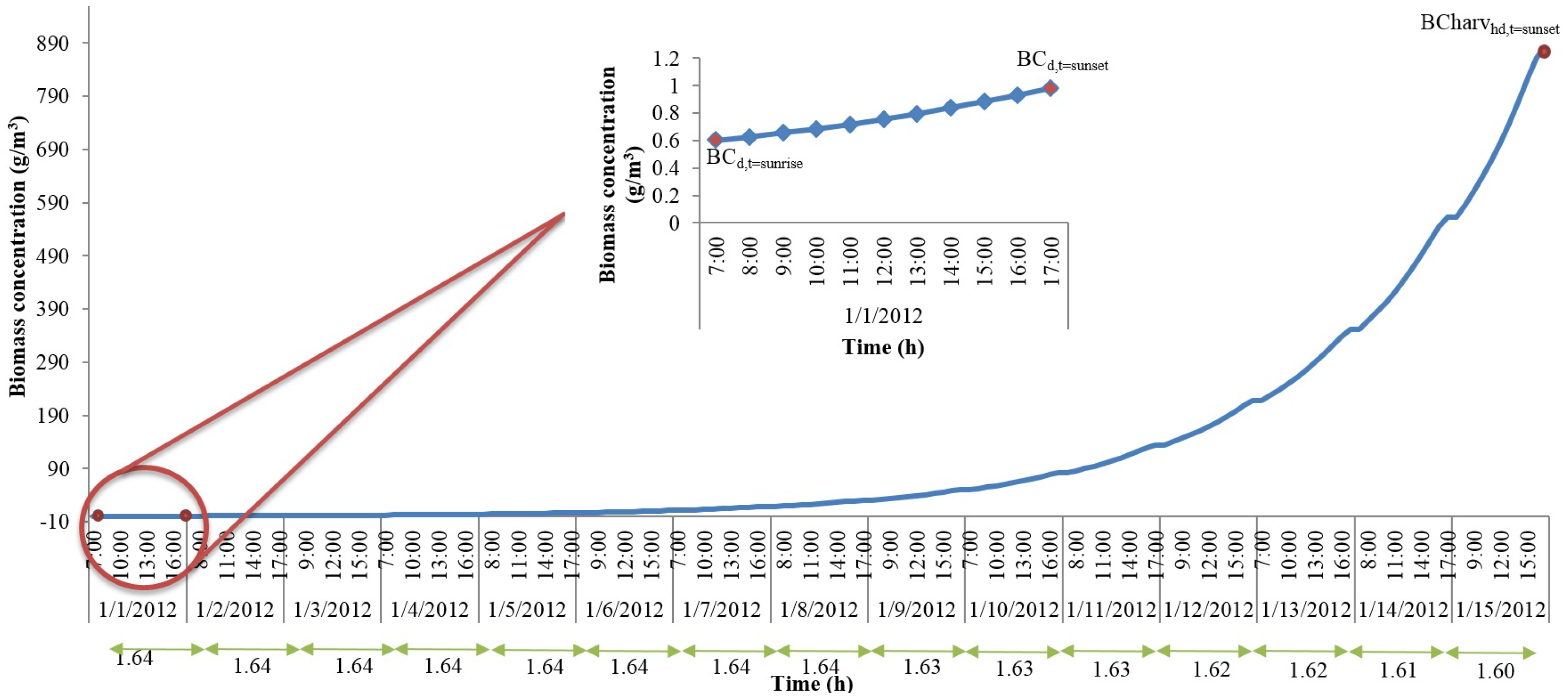
Figure 2 shows changes in biomass concentration until harvest for the 15-day solution for the month of January. The x-axis shows day light time (sunrise through sunset) in a given day while y-axis shows the biomass concentration. Biomass concentration was constrained such that at sunrise of day-1, initial seeding took place. As the day progressed, the biomass concentration kept increasing until it reached the time of sunset. The concentration at sunrise of the next days was set equal to the concentration at sunset of the previous days until harvest (this assumption would yield a theoretical upper bound for the algal biomass production). The ratio of biomass concentration at sunrise to that at sunset is calculated for each day, and these ratios are given in Figure 2 at the bottom of x-axis. As can be seen from Figure 2, the ratios do not change significantly. The constant ratio allows the development of an expression that calculates the biomass concentration at harvest if the biomass concentrations at the time of seeding (which is a parameter for our original model and should be known) and at the time of sunset (which can be obtained if the dynamics of one representative day is included in the optimization model) are known. This expression is given in Equation (53).

$$BChar{v}_{hd}\left(t=sunset\right)=BC\left(t=sunrise-1\right)\cdot {\left[\frac{BC\left(t=sunset\right)}{BC\left(t=sunrise-1\right)}\right]}^{harvP}$$

(53)

In Equation (53), BCharv_hd(t = sunset) is the biomass concentration at the time of harvest, BC(t = sunrise–1) and BC(t = sunset) are the biomass concentrations at sunrise and sunset of the representative day, and harvP is the harvest period.

The above relation can be extended to production variables as well. Equation (54) relates accumulation of algae biomass, Xharv_c,hd(t), from the first day of harvest period to the last day of harvest period, to mass produced at sunrise and sunset, X_c(t), and harvest period, harvP. Here, X_c(t), (g) is the hourly production of the component c produced in a raceway pond on representative day.

$$\begin{array}{c}Xhar{v}_{c,hd}\left(t=sunset\right)=X_c\left(t=sunrise-1\right)\cdot {\left[\frac{X_c\left(t=sunset\right)}{X_c\left(t=sunrise-1\right)}\right]}^{harvP}\\ \forall c\in \left\{DA,WIA\right\}\end{array}$$

(54)

now, the total annual production can be calculated by the sum of all the accumulated biomass, Xharv_c,hd(t), from the sunrise of the first day to the sunset of the last day of harvest period times the number of harvest cycles, harvC, in a month as shown in Equation (55). This equation replaces Equations (27) and (28) in our model.

$$D_{c,y}={\displaystyle \sum _{hd=1}^{12}harvC}\cdot Xhar{v}_{c,hd}\left(t=sunset\right)\forall y,\forall c\in \left\{DA,WIA\right\}$$

(55)

Equations (43) and (44) can be rewritten as Equations (56) and (57) for calculating the energy requirements when considering only the times between sunrise and sunset for the whole year. In Equations (56) and (57), the multiplication with 30 converts the daily energy requirements to annual energy consumption.

$$EPP=30{\displaystyle \sum _{d=1}^{12}{\displaystyle \sum _{t=sumrise}^{sunset}PP(d,t)}}$$

(56)

$$EPW=30{\displaystyle \sum _{d=1}^{12}{\displaystyle \sum _{t=sumrise}^{sunset}PW(d,t)}}$$

(57)

Annual industrial water requirements, Indwater (m³), to run a raceway pond and to compensate for the evaporated water is calculated via Equation (58).

$$Indwater=\frac{1}{\rho }\left[{\displaystyle \sum _{t}me(t)\cdot SA}\right]+\left(harvP\cdot harvC\cdot V\right)$$

(58)

Equations (2) through (5), (7) through (26), (29) through (42), and (45) through (58) form a nonlinear programming formulation representing open-channel raceway pond design. The model is implemented in General Algebraic Modeling System (GAMS) version 24.2.1(GAMS Development Corporation, NW Washington, DC, USA, 2013), and solved using CONOPT version 3.15 M (ARKI Consulting & Development, Bagsvaerd, Denmark, 2013) with the default optimality tolerance of 1 × 10⁷. CONOPT option Rtmaxv = 1 × 10³⁰ was used as the upper limit on the variables. Maximum number of domain errors was set to 1000 and maximum number of solver iterations was set to 5000. Because CONOPT is a local optimization solver, we used a multiple-start approach, where the model variables were initialized to different values generated using Latin Hypercube Sampling technique, in an effort to find the global solution.

6. Case Study

For the case studies, the optimum raceway pond geometries are obtained for each combination of two species (P. tricornutum and I. galbana) and four locations (Tulsa, USA; Hyderabad, India; Cape Town, South Africa; and Rio de Janeiro, Brazil). The case study data for the species and model parameters are shown in

Table A1. Summary of species dependent parameters [41].

Species	Percentage of Dry Algae (%)	Lipid Content (dw)	Light Absorption Coefficient of Biomass (m2·g−1) [42]	Constant (μE·m−2·s−1)
P. tricornutum	20	0.31	0.0369	114.67 [42]
I. galbana	30	0.21	0.0369	170.68

and

Table A2. List of the model parameters.

Scalar	Value	Unit
ηPW	0.17
EmpA	0.16 [43]
EmpB	0.19 [43]
Ephoton	225.3	kJ·mol−1

of Appendix. The weather data–maximum temperatures, minimum temperatures, relative humidity and wind velocity for locations are presented in

Table A3. List of average temperature parameters for the locations.

Date	Tulsa		Hyderabad		Cape Town		Rio de Janeiro
	Tmaxl,d (°C)	Tminl,d (°C)	Tmaxl,d (°C)	Tminl,d (°C)	Tmaxl,d (°C)	Tminl,d (°C)	Tmaxl,d (°C)	Tminl,d (°C)
January 2012	10	−2	32	16	27	16	28	22
February 2012	8	2	34	18	25	15	30	23
March 2012	17	10	38	21	23	14	29	23
April 2012	20	13	39	25	22	14	28	23
May 2012	25	17	42	28	19	11	26	20
June 2012	29	20	36	25	18	11	26	21
July 2012	35	22	31	23	17	10	25	20
August 2012	31	20	31	23	16	10	26	19
September 2012	27	18	32	23	19	12	27	19
15 October 2012	16	10	32	20	21	13	29	21
15 November 2012	12	3	31	18	22	13	26	21
15 December 2012	9	0	32	16	26	15	32	24

and

Table A4. List of average relative humidity and wind velocity parameters for the locations. They are taken the same for all times of the day.

Date	Tulsa		Hyderabad		Cape Town		Rio de Janeiro
	RHl,d(t)	WVl,d(t) (m·s−1)	RHl,d(t)	WVl,d(t) (m·s−1)	RHl,d(t)	WVl,d(t) (m·s−1)	RHl,d(t)	WVl,d(t) (m·s−1)
January 2012	0.597	8.705	0.520	5.866	0.755	19.63	0.813	11.06
February 2012	0.698	7.581	0.429	6.393	0.726	15.83	0.753	11.77
March 2012	0.740	8.323	0.311	6.292	0.803	17.10	0.805	12.81
April 2012	0.765	6.847	0.446	5.088	0.728	18.72	0.829	11.74
May 2012	0.758	6.817	0.308	8.592	0.809	14.03	0.793	10.13
June 2012	0.750	6.088	0.489	15.03	0.777	12.87	0.832	10.58
July 2012	0.575	5.789	0.687	14.74	0.744	18.25	0.779	10.31
August 2012	0.597	5.186	0.715	12.00	0.733	20.06	0.749	11.38
September 2012	0.629	6.618	0.693	10.35	0.718	16.62	0.732	12.86
15 October 2012	0.711	6.775	0.565	6.608	0.711	23.42	0.725	12.84
15 November 2012	0.723	5.840	0.559	6.045	0.733	19.12	0.833	12.51
15 December 2012	0.730	7.563	0.455	6.015	0.755	22.51	0.762	12.64

of Appendix. The breakdown of total capital investment coefficient (TCI_l) and total production cost coefficient (TPC_l) is shown in Section 6.1. In this work, all the cost coefficients have been inflated to the year 2012. The annual algae biomass demand in Equation (25) is five tons per annum. The harvest period and harvest cycle in each month were taken to be six days and five cycles, respectively. It was assumed that the raceway is seeded just before sunrise after each harvest to yield a biomass concentration of 0.6 g·m⁻³ [11].

Sensitivity analysis is performed on the best case results, i.e., species and location combination that yielded the lowest net present cost, to understand the influence of harvest time, demand, channel length to width ratio, and biomass initial seeding concentration on the optimum solution.

6.1. Economic Assumptions

The financial assumptions applied in the present study are summarized below. These costs are taken from literature for the year 1996 [35].

■

Estimation of capital investment cost (TCI_l)

□

Direct costs: They include site preparation, grading, compaction; pond levees, geotextiles; mixing (paddle wheels); CO₂ diffusers; harvesting; flocculation; centrifugation; water and nutrient supply system; waste treatment (blow down); building and structures; electrical supply and distribution; instrumentation and machinery; and land costs [35]. The total direct costs add to $63,700/ha

□

Indirect costs: Engineering and contingency = 15% of direct costs excluding land costs = $9,255/ha

□

Fixed-capital investment = direct costs + indirect costs = $72,955/ha

□

Working capital = 15% of total capital investment

□

Total capital investment = fixed-capital investment + working capital = $85,829/ha

□

10% rate of return

□

10 years plant life

□

Straight line depreciation

□

Cost index for 2012

■

Estimation of total production cost (TPC_l)

□

Manufacturing costs: They include utilities–power required for harvesting, processing, lighting up buildings; nutrients; flocculants; waste disposal; maintenance and repairs = 5% of fixed-capital investment; operating supplies = 15% of maintenance and repairs; depreciation = fixed-capital investment/number of recovery years; local taxes and insurance = 4% of fixed-capital investment; financing = 5% of total capital investment; and labor and overhead costs. The total manufacturing costs add to $28,600.08/ha/year

□

General expenses = 20% of total production cost = $7,150.02/ha/year

□

Total production cost = manufacturing costs + general expenses = $35,750.1/ha/year

These costs have been inflated to current values depending on chemical engineering cost index. Hence, the total capital investment (TCI_l) was calculated as $13.144 m⁻² and total production cost (TPC_l) was calculated as $5.475 m⁻²·year⁻¹. Here, cost index for 1996 and 2012 were taken as 382 and 585, respectively. Cost of electricity and water are taken from literature [35] as ElCost_l: 0.07 $ (kW·h)⁻¹ and WtCost_l: 3.18 $ (1000 gal)⁻¹, respectively. It should be noted that these economic parameters are taken same for all locations to understand the sole influence of algae species, geographical location, and raceway pond geometry on one another.

6.2. Problem Statistics and Solution Approach

The resulting optimization problems (NLPs) have 4360 variables and 4219 equations for the case of Hyderabad location; 4484 variables and 4339 equations for the case of Tulsa location; 4391 variables and 4249 equations for the case of Cape Town location; and 4360 variables and 4219 equations for the case of Rio de Janeiro location. The length of the day (the period between sunrise and sunset) differs from location to location due to the difference in latitude, longitude, and time zone. This causes the variation in the total number of variables and equations. Based on these, the degrees of freedom is three: channel depth, channel width, and biomass concentrations. Note that biomass concentration is a time-dependent variable, and its size depends on the location.

The values of channel depth, channel width, and biomass concentrations were initialized using Latin Hypercube Sampling technique. The rest of the model variables were calculated using these initializations. This sampling method is chosen because it spreads the sample points more evenly across all possible values. It partitions each input distribution into N intervals of equal probability, and selects one sample from each interval. In our model, we generated 100 samples to initialize the decision variables. Each of the eight cases was solved 100 times using the Latin Hypercube initializations. As noted before, to obtain a local solution, the variables of the model should be initialized to a feasible or a near-feasible solution. An iterative initialization scheme is implemented in GAMS version 24.2.1 to draw model initialization to a feasible or a near-feasible solution. The model is first attempted to be solved with an initialization from the Latin Hypercube samples. If it is solved to optimality, the model is initialized with the next Latin Hypercube sample. If the model is not solved to optimality, the model is initialized using the values of channel depth and channel width of the feasible or infeasible solution obtained by the CONOPT version 3.15 M. The biomass concentrations are initialized to that at sunset of the first representative day. The initializations for the rest of the variables are calculated based on these three variable values. This process is repeated for eight iterations or until an optimum solution is obtained. If an optimum solution is not obtained at the end of eight iterations, the initialization scheme moves to the next Latin Hypercube initialization point. The solutions presented in the next section (Section 6) are the local optimum solutions that yielded the lowest costs for each algae species and location pair.

7. Results and Discussion

Table 1. Summary of results for the eight Nonlinear Programming (NLP) Models.

Case	Z ($)	CD (m)	CW (m)	Length (m)	SA (m2)	V (m3)	Iavg (μE·m−2·s−1)	Uavg (m·s−1)	BC (g·m−3)	Μ (h−1)	PrV (g·m−3·Day−1)	PrA (g·m−2·Day−1)	Tpond (°C)
1(P.tricornutum, Tulsa)	179,080	0.43	2.57	300	1538	656	1457	0.102	51	0.042	8.448	3.602	15
2(P.tricornutum, Hyderabad)	96,566	1.5	0.56	300	337	505	2060	0.117	66	0.060	10.972	16.458	23
3(P.tricornutum, Cape Town)	493,900	0.81	4.74	300	2822	2274	1797	0.100	15	0.040	2.436	1.963	16
4(P.tricornutum, Rio de Janeiro)	102,970	0.79	0.997	300	597	468	1707	0.100	71	0.062	11.829	9.274	23
5(I.galbana, Tulsa)	131,660	0.3	2.24	300	1342	403	1463	0.114	122	0.035	20.313	6.094	15
6(I.galbana, Hyderabad)	61,109	0.3	0.95	300	571	171	2125	0.100	286	0.070	47.74	14.323	24
7(I.galbana, Cape Town)	2,215,200	1.49	13.64	300	8022	11954	1773	0.100	4	0.024	0.684	1.019	15
8(I.galbana, Rio de Janeiro)	84,363	0.42	1.19	300	713	297	1724	0.100	165	0.063	27.506	11.474	24

summarizes the raceway pond geometries and averages of important culture properties for eight case studies. The table allows us to identify the best combination of species, location, and pond geometry, and helps in identifying the promising alternatives. The variables that are given in Table 1 are the net present cost (Z) which is the objective function for each case study; pond geometry such as the channel depth (CD), channel width (CW), pond length (length), Surface area occupied by the pond (SA) and volume occupied by the pond (V); average annual physical properties such as average irradiance inside the pond (I_avg), channel velocity (U_avg), and pond temperature (T_pond); average annual culture properties such as biomass concentration (BC) and specific growth rate (µ); and average daily productivities such as volumetric productivity (PrV) and areal productivity (PrA). Average annual culture and physical properties are highlighted here to give an idea of how much the average values would be for a given year. However, the culture properties and physical properties fluctuate on a daily basis based on the climatic conditions. These fluctuations are shown via Figure 3 through 8.

The results from Table 1 reveal that the geometry of the open-channel raceway pond is different for different algae species and geographical location because the culture properties such as biomass concentration, growth rate, and biomass productivities change with respect to the algae species and local climatic conditions. The optimal raceway pond designs presented in Table 1 suggest that amongst the two algae species, I. galbana species, and amongst the four locations, Hyderabad, India, (Case 6) meets the annual demand of 5 tons algae biomass at the minimum net present cost of $61,109 for a plant life of 10 years. The cost of dry algae was found to be $3.28 kg⁻¹. It can be observed that I. galbana species require shallower and wider ponds and Hyderabad, India location requires shallower and narrower ponds for growing algae.

I. galbana species is selected over P. tricornutum species for algae biomass production because I. galbana species has higher light extinction coefficient, I_k. This enables higher light absorption inside the pond which triggers higher productivity and lower costs. This behavior can be observed in Table 1. Cases 5 through 8 where I. galbana species is cultured requires smaller pond volumes when compared to Cases 1 through 4 where P. tricornutum species is cultured, except for Case 7. We hypothesize that the solution of Case 7 is a bad local minima.

Hyderabad, India is selected over the others for algae biomass production because the average irradiance inside the pond at this location triggers higher biomass concentration, growth rates, and productivities compared to that at other locations. As expected, at higher average pond temperatures, the average algae growth rates are higher, and higher average biomass concentrations in the pond lead to lower biomass production costs (Table 1). Cases 2 and 5 where I. galbana and P. tricornutum species are cultured in Hyderabad, India, require smaller pond volumes when compared to other cases.

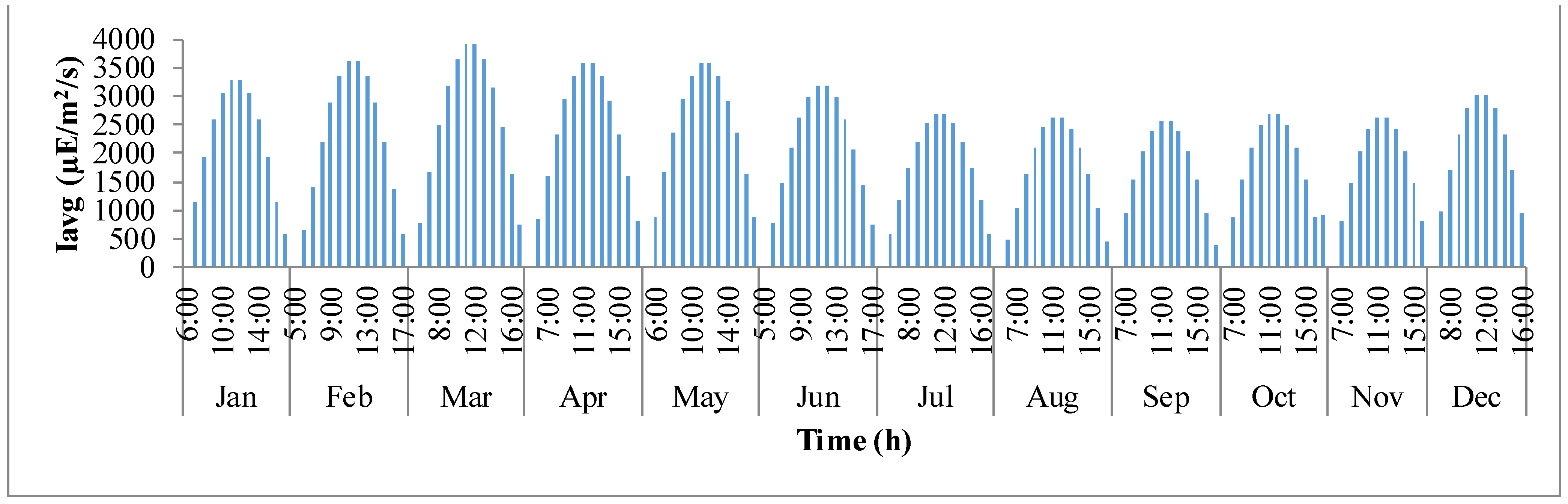
Figure 3 shows the variation in sunlight at the best location to grow algae, i.e., Hyderabad, India. The x-axis defines the clock times in 24 h format for each representative day of the month, and the y-axis is the solar irradiance (µE·m⁻²·s⁻¹). It is evident that as the day progresses, sunlight keeps increasing until mid-day and later decreases as it comes close to nightfall. It can also be observed that as summer approaches, solar irradiance tends to build up until the month of March and later declines as winter approaches. Figure 4 shows how average light intensity (I_avg) inside the pond varies with day light time of the representative day for I. galbana species cultured in Hyderabad, India. The x-axis defines the times in a 24 h format for each representative day of the month and y-axis is the average light intensity (μE·m⁻²·day⁻¹). It follows a trend similar to that of solar irradiance (I_o). It can be observed that in a representative day, the average light intensity inside the pond gradually increases from the time of sunrise until mid-day and later decreases as the sun goes down. This trend continues for all representative days of the year. However, on an overall scale, the light intensity is maximum inside the pond during the months of February, March, April, and May. 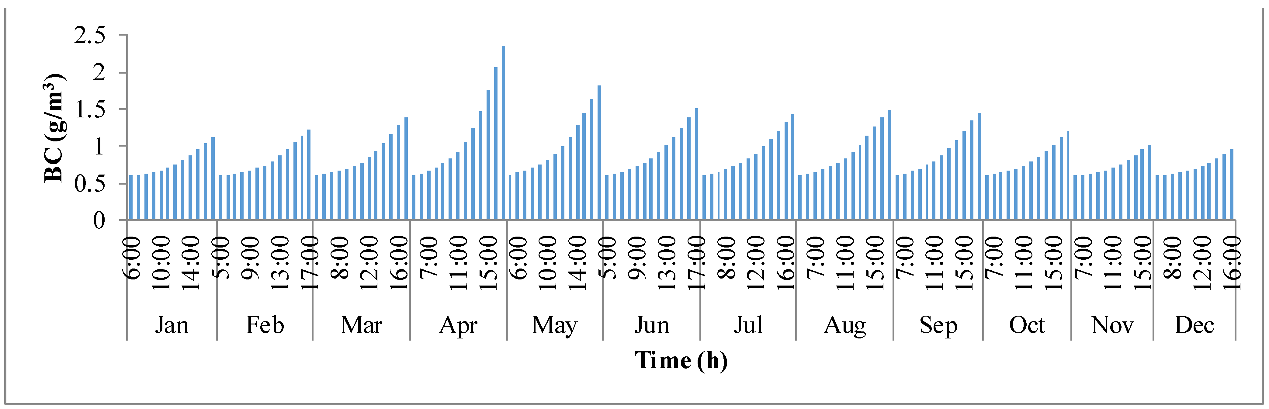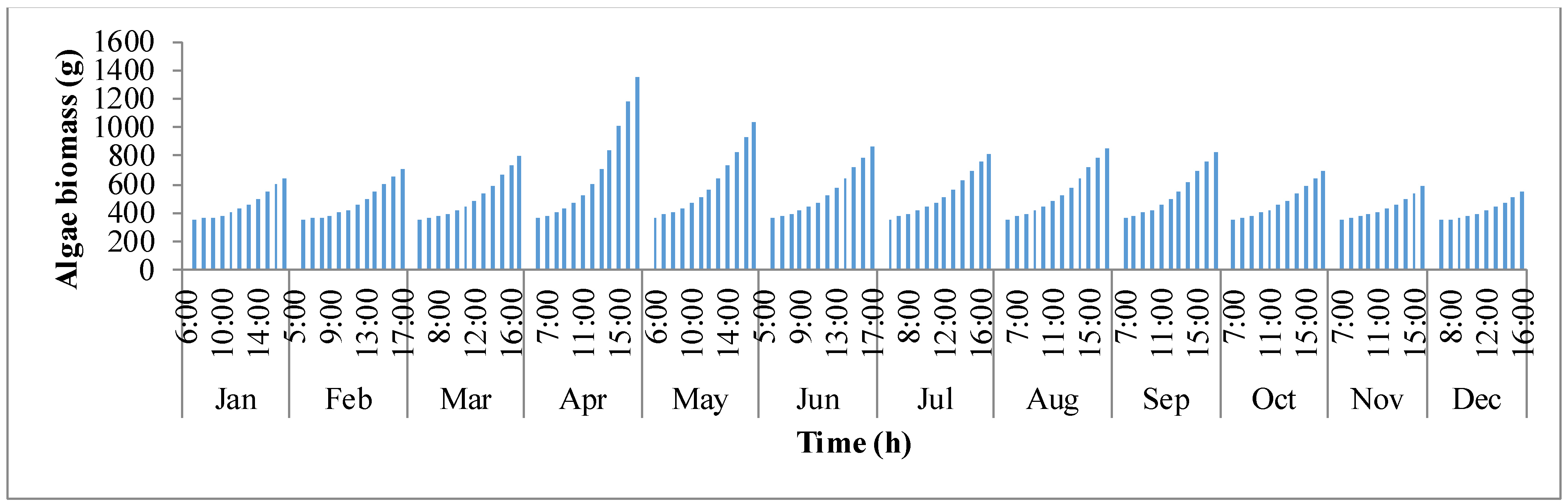Figure 5 shows the biomass concentration profile (g·m⁻³) in the same format. On each representative day just before sunrise, biomass concentration is initiated to 0.6 g·m⁻³. During the course of the day with sunlight, the concentration in the pond builds up continuously until it reaches sunset. The concentration has rapidly raised from sunrise to sunset in the months of summer when compared to the winter months. Figure 6 shows the trend in biomass production (X_f and X_g). The x-axis shows day light time (sunrise through sunset) in a given day while y-axis shows the biomass production. It follows the same trend as biomass concentration. It is clear that as production rises, concentration of biomass inside the pond rises. 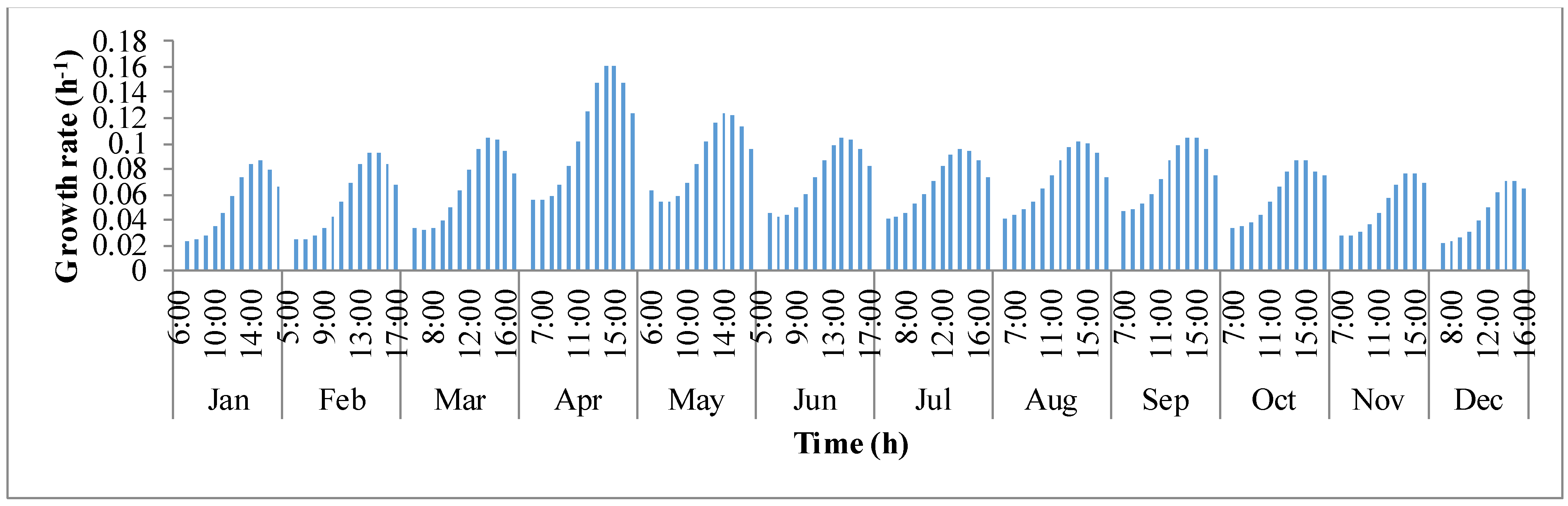In Figure 7, x-axis is the clock times in 24 h format for each representative day of the month and y-axis is the growth rate (μ). For a given day, growth rate of algae biomass tends to increase in the first few hours until mid-day and later decreases. This behavior of deteriorating growth rate is mainly due to the decrease in the pond temperature in the afternoon hours. Algal growth rate is rapid in the summer months of March, April, and May because temperature of the pond oscillated around the optimal growth temperature of I. galbana (~27 °C).

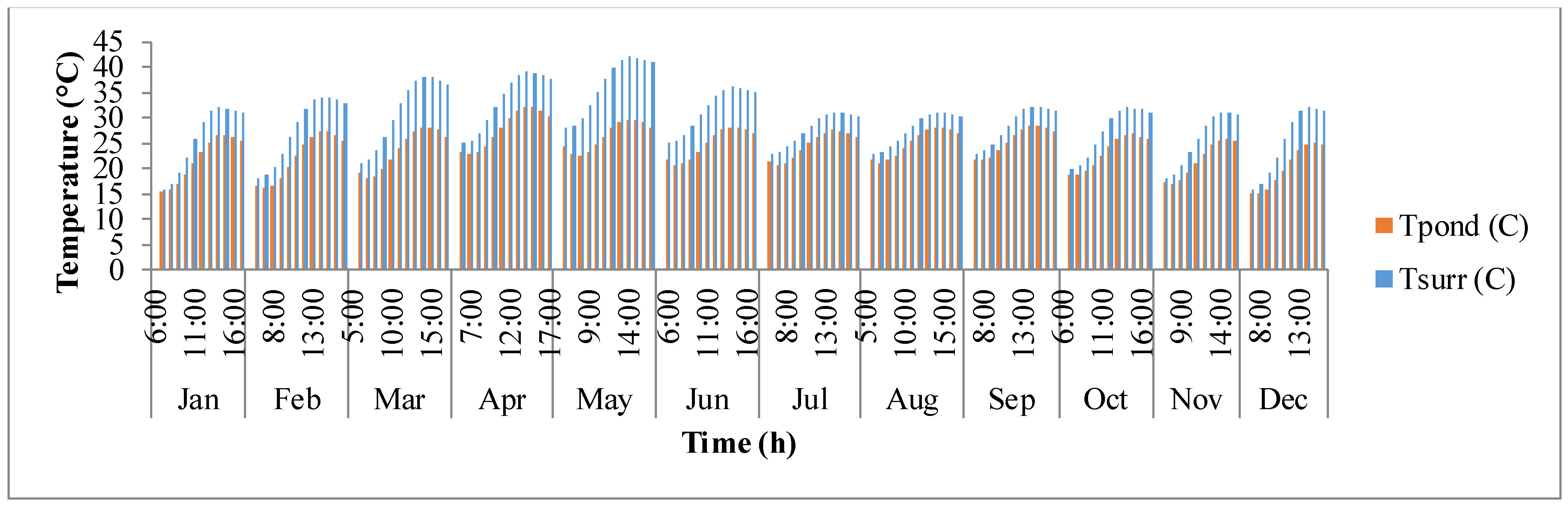
Figure 8 shows the fluctuation of surrounding temperature (T_surr) and raceway pond temperature (T_pond) with time. Surrounding temperature depends on maximum and minimum temperature of the day, longitude, and time zone. It rises from sunrise until mid-day and then after goes down as the sun goes down. Temperature of the pond is driven by surrounding temperature and thermal gains/losses in the pond due to solar radiation, air radiation, pond radiation, evaporative heat transfer, convective heat transfer, and heat transfer due to inflow water. It is also dependent on the growth rate of algae as shown in Equations (4) and (5). The temperature of the pond rises as the day progresses and reaches a maximum after which it decreases. The decrease in pond temperature is mostly due to the cooling effects of evaporation. It can be observed that the surrounding temperature and pond temperature are high during the warmer months of March, April, and May.

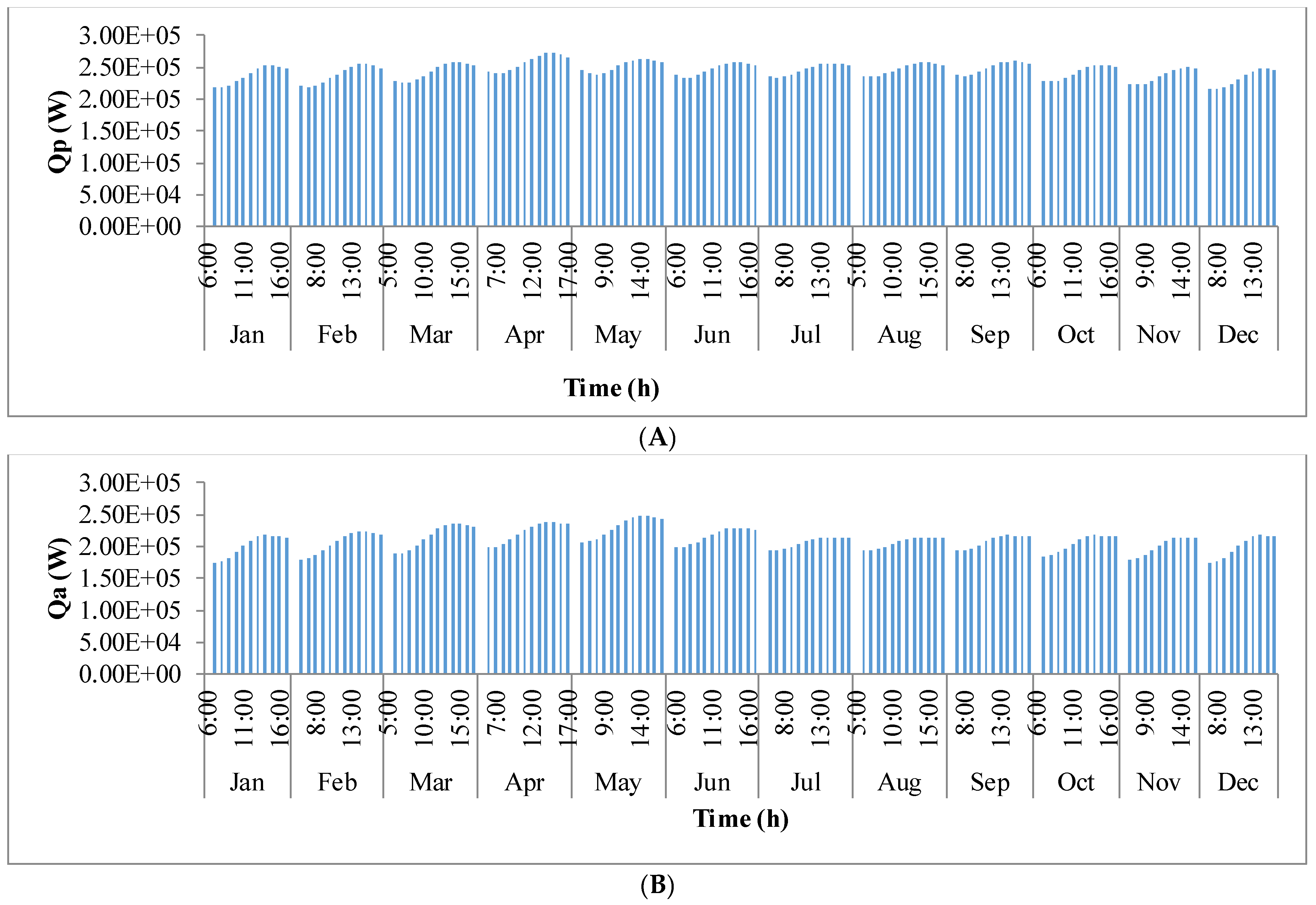
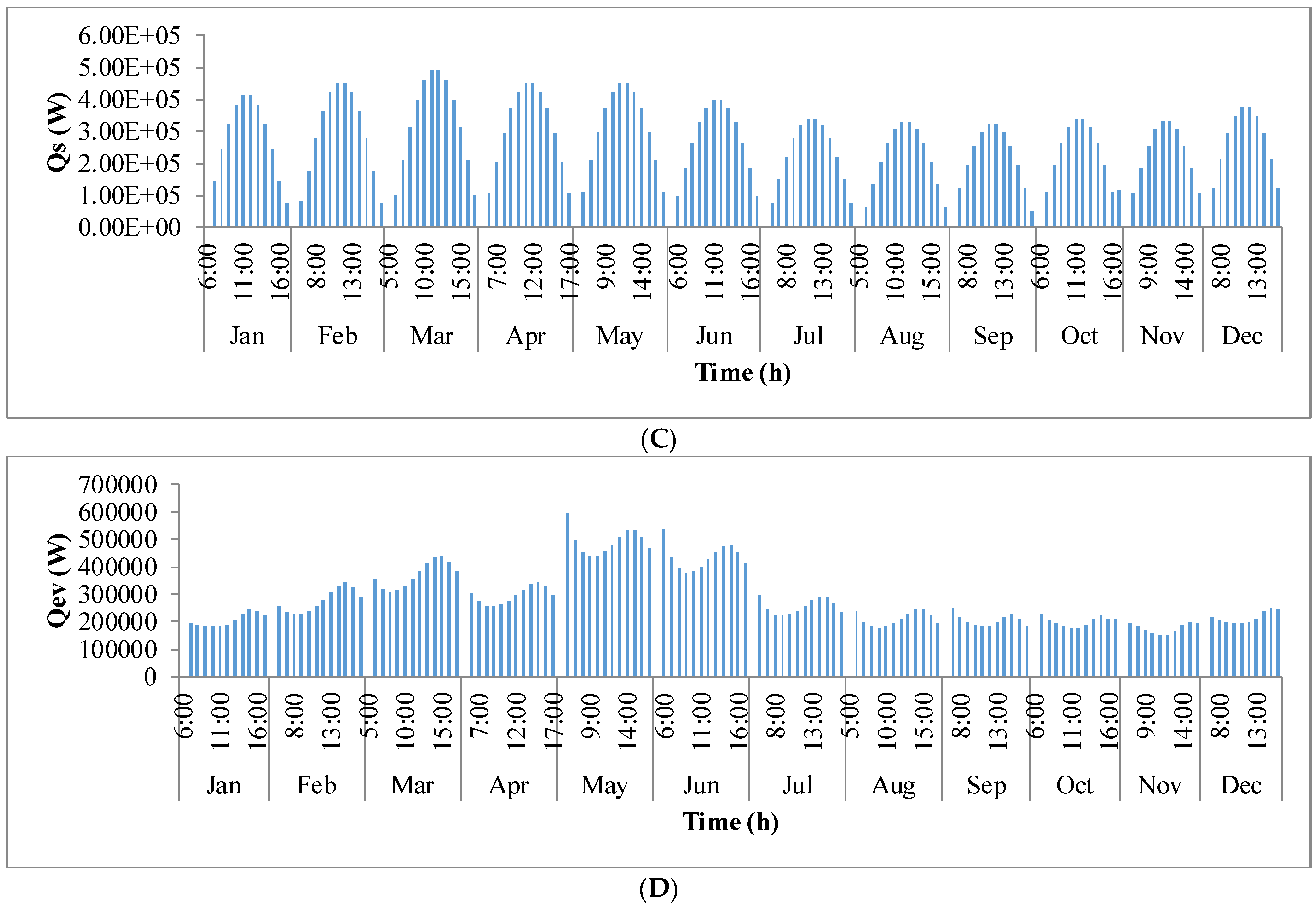
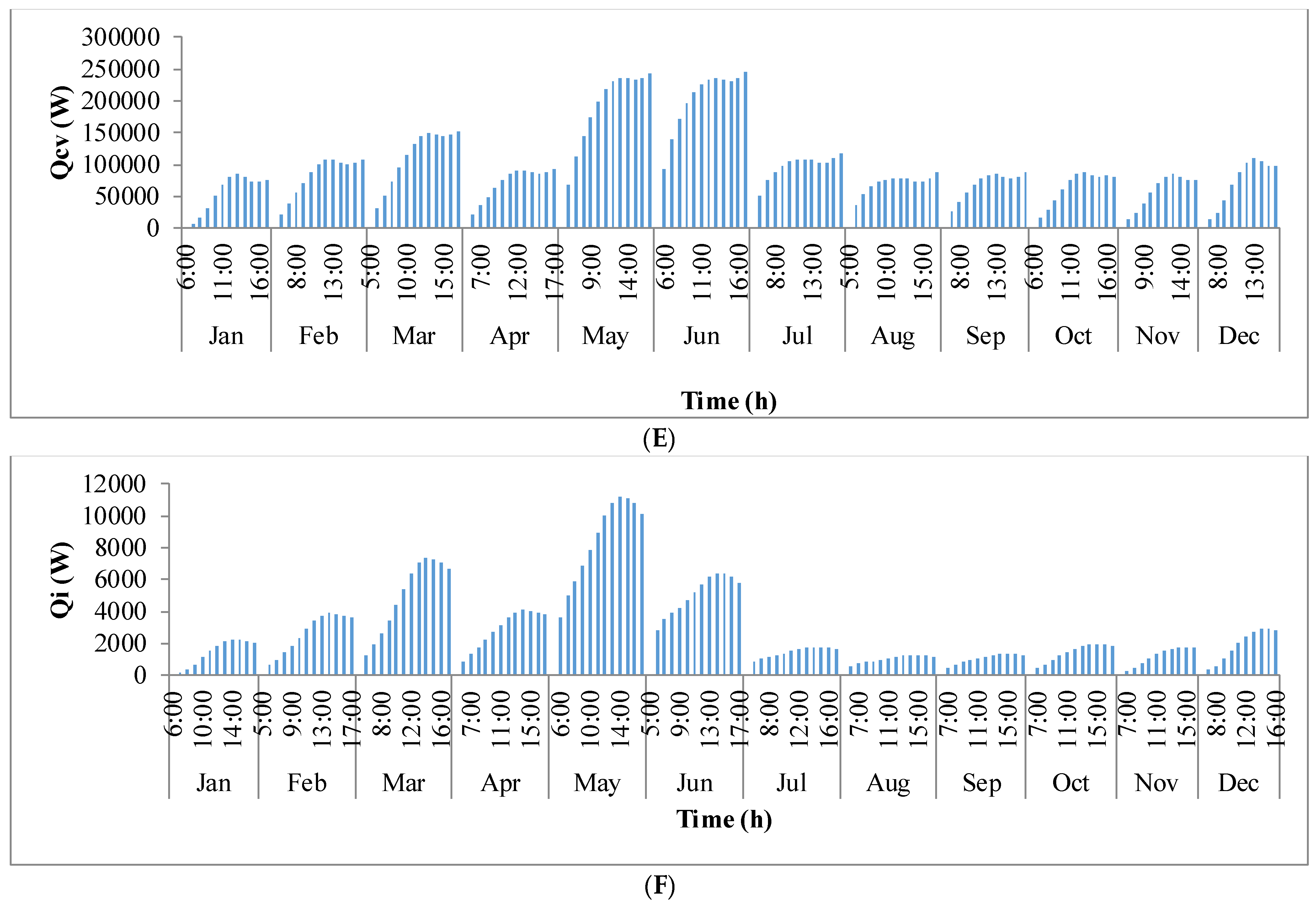
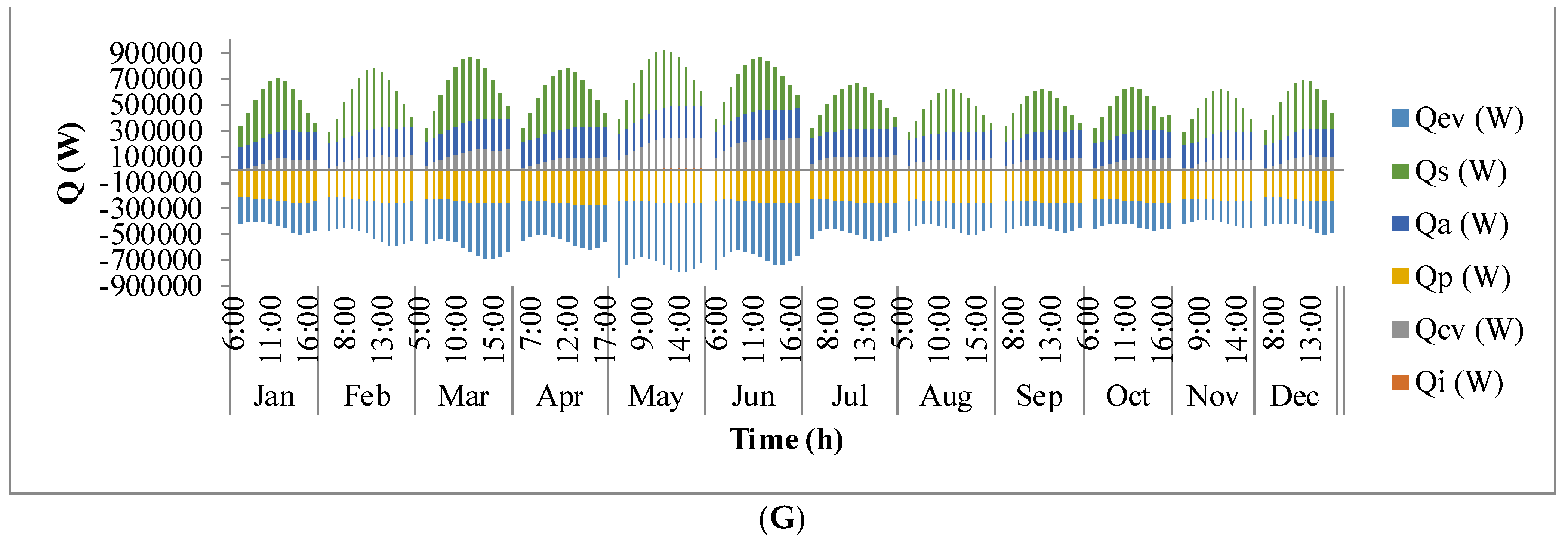
Figure 9 shows the annual variation in heat flow in open-channel raceway ponds. The x-axis shows the representative days of the respective months in a year and y-axis shows the six heat fluxes considered for energy balance in the pond: radiation from the pond (Q_p), radiation from the air (Q_a), radiation from the sun (Q_s), evaporative heat flux (Q_ev), convective heat flux (Q_cv), and inflow heat flux (Q_i). Radiation from the pond (Q_p) depends on pond temperature (T_pond). Hence, rate of heat flow from the pond, (Figure 9A), follows a similar trend as pond temperature in Figure 8. It can be observed that at the beginning of the day, less radiation is emitted by the pond and as the day progresses, the pond temperature increases and so does the radiation from the pond. Radiation from the air (Q_a) (Figure 9B) follows a similar trend as surrounding temperature (T_surr) (Figure 8), and radiation from the sun (Q_s) (Figure 9C) follows a similar trend as irradiance at the location (I_o) (Figure 3) as they depend on one another. It can be observed that evaporative heat flux (Q_ev) (Figure 9D) is dominant in the month of May when the surrounding temperature is high. The increase in the heat transfer due to evaporation during this month has led to cooling in the pond, and hence, there is a decrease in the pond temperature. Evaporation increases from sunrise to mid-day and later decreases with the course of the day. However, in summer months, at sunrise when the surrounding temperature is higher than the pond, evaporation is high. Rate of heat flow due to convection (Q_cv) (Figure 9E) is higher in May and June similar to that of evaporation heat flux. Inflow heat flux (Q_i) (Figure 9F) is the rate of heat transfer between the water that is added to the pond, that is lost during evaporation, and the pond water itself. It can be observed that during the months of May and June, when the rate of evaporation is high, the pond water is relatively cooler. The water added to the pond is assumed to be at the surrounding temperature. Hence, heat transfer from inflow water to the pond water is high during those months. Among all the heat fluxes, rate of heat transfer due to evaporation plays a major role in determining the temperature of the pond.

Sensitivity Analysis

Sensitivity analysis was performed on the best case, i.e., Case 6, to understand the influence of model parameters on the overall design of raceway pond and on the cost of algae biomass production. The studied parameters include the harvest times (harvP), upper bound on pond length, lower bound on channel depth, and initial biomass concentration (BCini).

Table 2. Summary of sensitivity analysis results by changing the harvest time.

Case	harvP	Z ($)	CD (m)	CW (m)	Length (m)	V (m3)	SA (m2)	Iavg (μE m−2·s−1)	Uavg (m·s−1)	BC (g·m−3)	μ (h−1)	PrV (g·m−3·Day−1)	PrA (g·m−2·Day−1)
6-SA1	1	1.2384 × 106	1.5	7.363	300	6557	4371	2061	0.114	1.25	0.059	1.247	1.871
6-SA2	2	1.1000 × 106	1.5	6.527	300	5819	3880	2061	0.117	2.81	0.059	1.405	2.108
6-SA3	3	6.8332 × 105	1.5	4.036	300	3611	2408	2061	0.117	6.79	0.059	2.264	3.396
6	6	6.1109 × 104	0.3	0.953	300	171	571	2125	0.100	286	0.0696	47.74	14.323
6-SA4	10	9.703 × 103	0.042	1.45	48	5.71	136	2140	0.131	14329	0.0635	1433	60

summarizes the results obtained by changing the harvest periods (harvP). The harvest periods studied are one, two, three, six, and ten days. It is evident that for longer harvest periods, harvP, i.e., when harvesting frequency is low, biomass concentration increases until the time of harvest because of accumulation of algae biomass, and hence, growth rates are high. It can also be observed from Table 2 that higher biomass concentrations require lower channel depth, which enables higher average light intensity inside the pond. Longer harvest periods are also marked by higher volumetric and areal productivities. The productivities are high because longer harvest periods allows accumulation of the product for longer time inside the pond. For the harvest period of 10 days, the channel depth, channel width, and channel length are 4 cm, 1.45 m, and 48 m, respectively. However, at the channel depth of 4 cm, evaporation occurs rapidly leading to biomass concentrations that are higher than 10,000 g·m⁻³. This would violate the model assumptions used in this work. In the current model, we assumed biomass concentrations to be below 10,000 g·m⁻³ in order to inhibit light attenuation due to dense cultures and keeping the fluid properties similar to that of water. Thus, from our analysis, the next better option to harvest the algae biomass is six days. Since, the length of the pond for a six day harvest period case was found to be the upper bound on pond length, sensitivity analysis was performed by increasing the upper bound of pond length to see its influence on the net present cost.

Table 3. Summary of sensitivity analysis results by changing the upper bound on length of pond.

Case	Upper Bound on Length (m)	Z ($)	CD (m)	CW (m)	Length (m)	V (m3)	SA (m2)	Iavg (μE·m−2·s−1)	Uavg (m·s−1)	BC (g·m−3)	μ (h−1)	PrV (g·m−3·Day−1)	PrA (g·m−2·Day−1)
6	300	6.1109 × 104	0.300	0.953	300	171	571	2125	0.100	286	0.0696	47.74	14.323
6-SA7	500	5.0875 × 104	0.331	0.449	500	149	449	2123	0.100	330	0.0709	54.950	18.216
6-SA8	1000	4.9553 × 104	0.372	0.299	688	153	411	2121	0.100	321	0.0710	53.434	19.895

summarizes the results obtained by changing the upper bound on pond length to see its influence on the net present cost and the culture properties. To meet the demand, as the upper bound on the pond length increases, the length tends to follow the upper bound. This results in an increase in the channel depth, making the channel width smaller. In the case of 6-SA6, as the pond becomes longer, channel width became smaller than channel depth, making the pond narrower and deeper. From our analysis, it is evident that longer ponds are economical for algae biomass production. However, report from National Renewable Energy Laboratory suggests that pond length should range between 10 and 300 m.

Table 4. Summary of sensitivity analysis results by changing the lower bound on channel depth.

Case	Lower Bound on CD (m)	Z ($)	CD (m)	CW (m)	Length (m)	V (m3)	SA (m2)	Iavg (μE·m−2·s−1)	Uavg (m·s−1)	BC (g·m−3)	μ (h−1)	PrV (g·m−3·Day−1)	PrA (g·m−2·Day−1)
6	0.3	6.1109 × 104	0.3	0.953	300	171	571	2125	0.100	286	0.0696	47.74	14.323
6-SA8	0.2	6.0927 × 104	0.278	0.979	300	163	586	2126	0.100	301	0.0700	50.18	13.944

summarizes the results obtained by changing the lower bound on channel depth. The case with lower pond depth leads to higher biomass concentration, growth rate, and productivity. This is the result of higher average light intensity inside the pond due to lower pond depths. From Table 4, it is clear that lower pond depth results in lower net present cost. Our analysis suggests that ponds depth should be kept as low as the pumping and construction allows.

Table 5. Summary of sensitivity analysis results by changing the initial biomass concentration in the pond.

Case	Bcini (g/m3)	Z ($)	CD (m)	CW (m)	Length (m)	V (m3)	SA (m2)	Iavg (μE·m−2·s−1)	Uavg (m·s−1)	BC (g·m−3)	μ (h−1)	PrV (g·m−3·Day−1)	PrA (g·m−2·Day−1)
6-SA5	0.1	2.9456 × 105	0.306	4.611	300	842	2748	2139	0.100	58	0.0708	9.71	2.975
6	0.6	6.1109 × 104	0.3	0.953	300	171	571	2125	0.100	286	0.0696	47.74	14.323
6-SA6	0.9	4.6405 × 104	1.5	1.925	42	240	160	2024	0.117	205	0.0526	34.10	51.152

summarizes the results obtained by changing the seeding, i.e., initial biomass concentration (BCini), in the pond at the time of sunrise. The case with higher initial biomass concentration proved to be economical, since higher initial seeding leads to better cultural properties such as average biomass concentration and productivities in the pond. As the initial biomass seeding concentration increases, the surface area required to meet the demand decreases. This leads to lower production costs of algae biomass. Therefore, the analysis suggests that higher initial seeding concentrations are required to obtain lower overall production costs. However, average light intensity inside the pond deteriorates with increasing biomass concentration because of mutual shading of the algae biomass.

8. Conclusions

In this paper, a dynamic optimization model is presented to estimate the best combination of algae species, geographical location, and raceway pond geometry by combining experimentally validated temperature, irradiance, and algae growth models. In order to represent the actual behavior of the outdoor raceway pond, the current model takes into account the diurnal pattern of sunlight, temperature fluctuations, the dynamic behavior of solar zenith angle, and mixing, which makes it more realistic compared to the other models in the literature.

The model is used to design the optimum raceway ponds for eight case studies, which considers two algae species (P. tricornutum and I. galbana) and four locations (Tulsa, USA; Hyderabad, India; Cape Town, South Africa; and Rio de Janeiro, Brazil). The combination of I. galbana-species, Hyderabad, India, and raceway pond geometry of 30 cm channel depth, about a meter channel width, 300 m in length, and a harvest interval of every six days provided cost effective production of algae biomass. Sensitivity analysis is performed to study the influence of model parameters on the overall design of raceway pond and the cost of algae biomass production. The results of the sensitivity analysis reveal that, among the studied ranges, longer harvest periods with higher initial biomass concentration and higher pond length to channel width ratio are recommended to minimize the net present cost of algae biomass production.