
Combining On-Line Characterization Tools with Modern Software Environments for Optimal Operation of Polymerization Processes


Abstract
:
1. Introduction
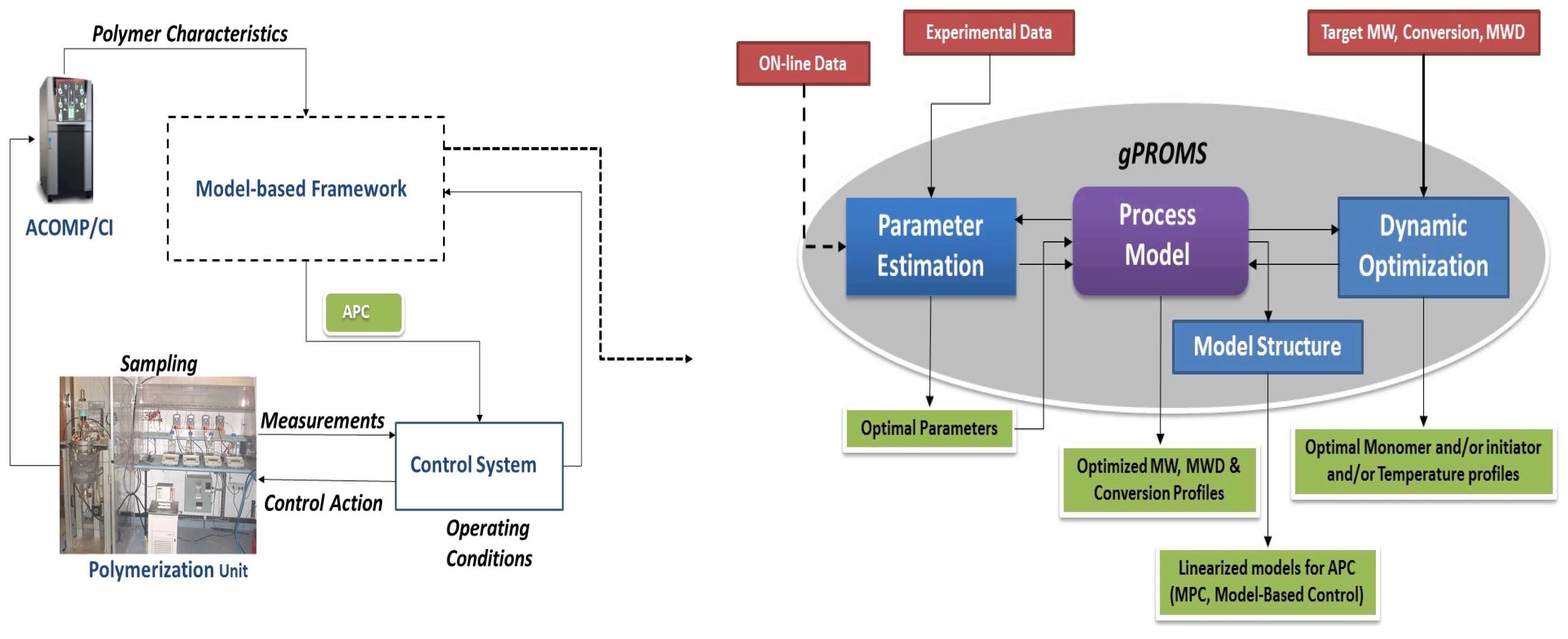
2. Model Centric Framework
2.1. Process Modelling
2.1.1. Reaction Mechanisms and Kinetic Equations
2.1.2. Formalism for Gel, Glass and Cage Effects in MMA Polymerization

| Parameter | MMA | Poly Methyl Methacrylate | Butyl Acetate |
|---|---|---|---|
| 𝛼 | 0.001 | 0.00048 | 0.001 |
| Tg(K) | 167 | 387 | # |
2.1.3. Molar Mass Distribution
2.1.4. Energy Balances
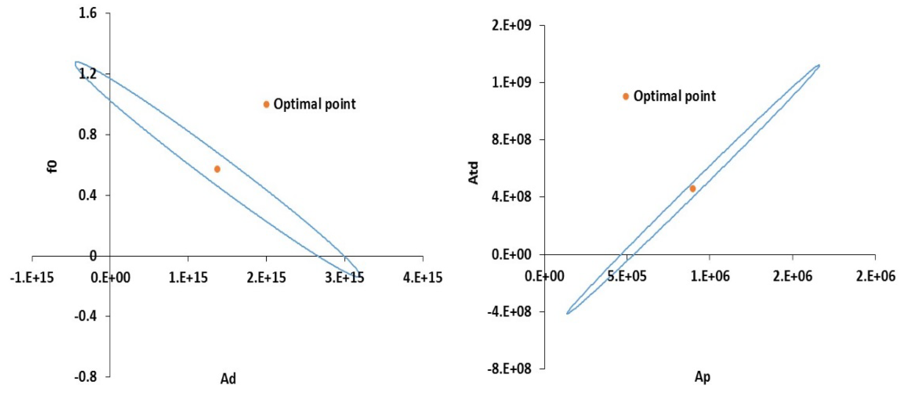
2.2. Parameter Estimation
- The overall duration.
- The initial conditions which are the initial loading of initiator, solvent and monomer.
- The variation of the control variables. For the batch experiment temperature is the only variable, while in semi batch both temperature and flow rate of monomer and/or initiator have to be considered.
- The values of the time invariant parameters.
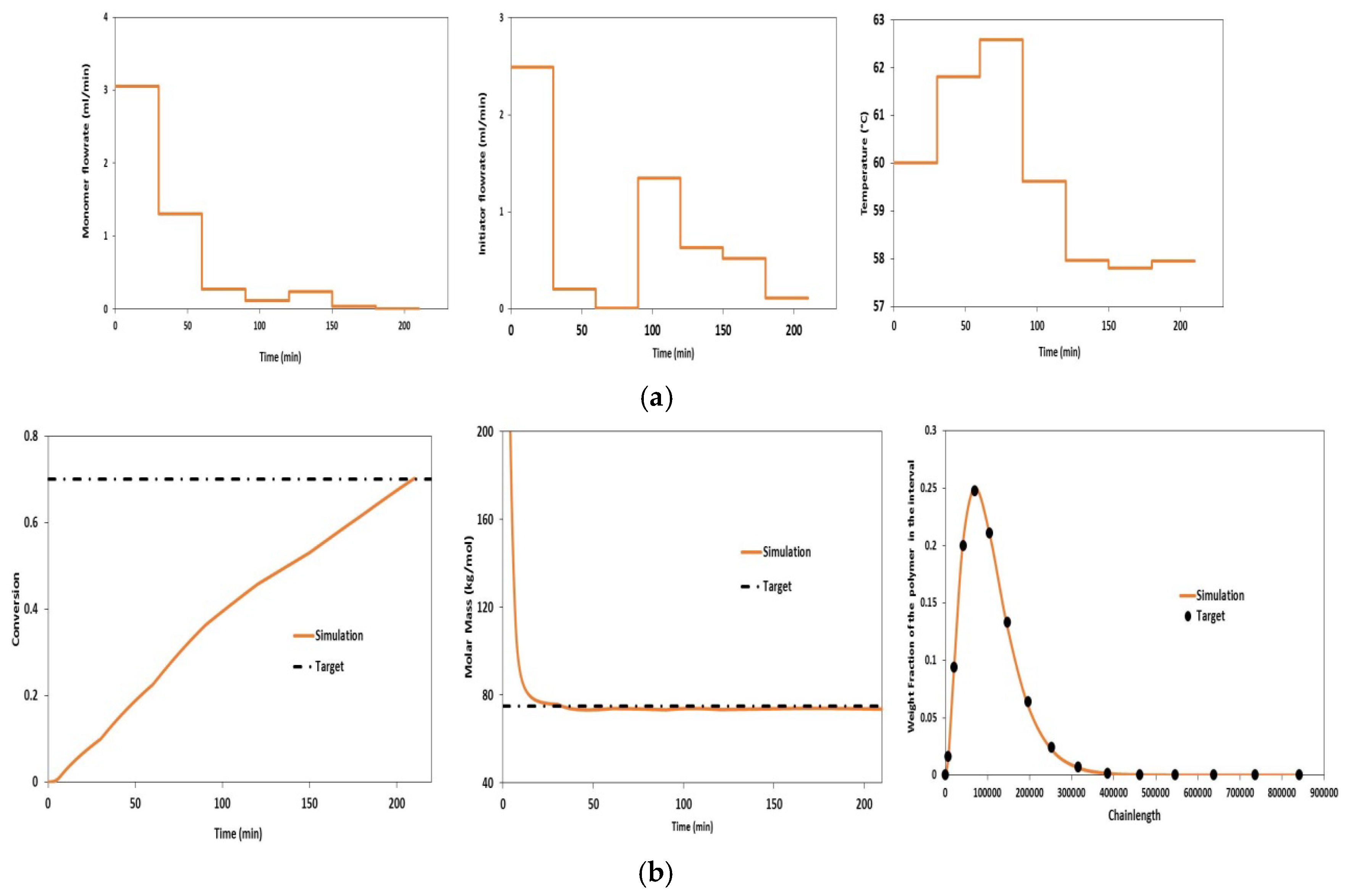
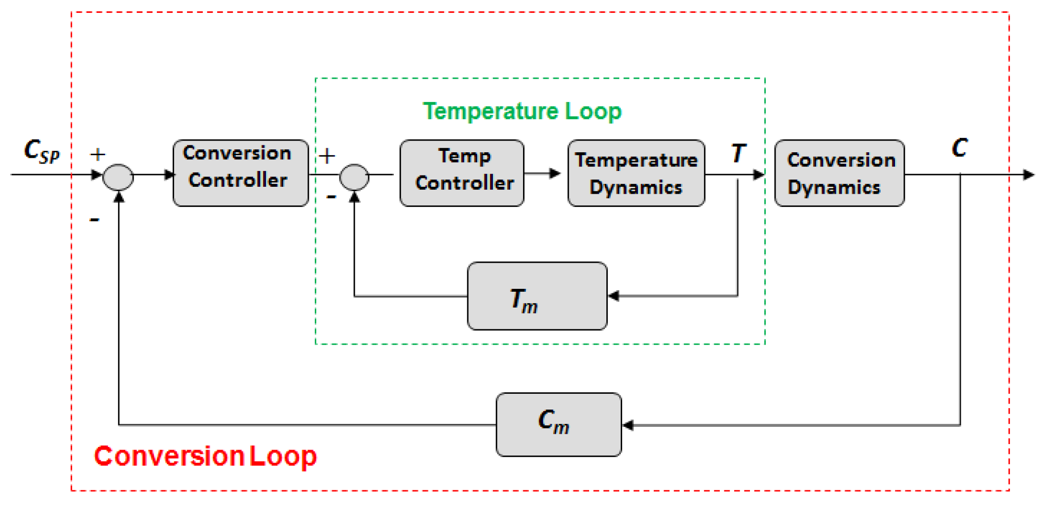
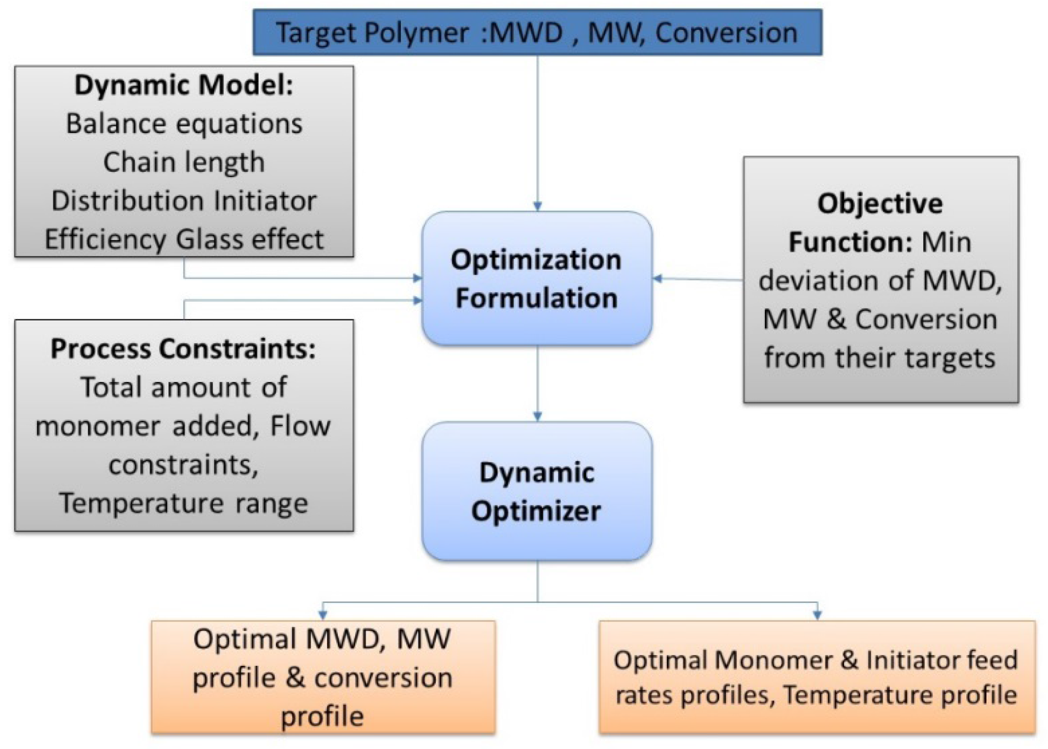
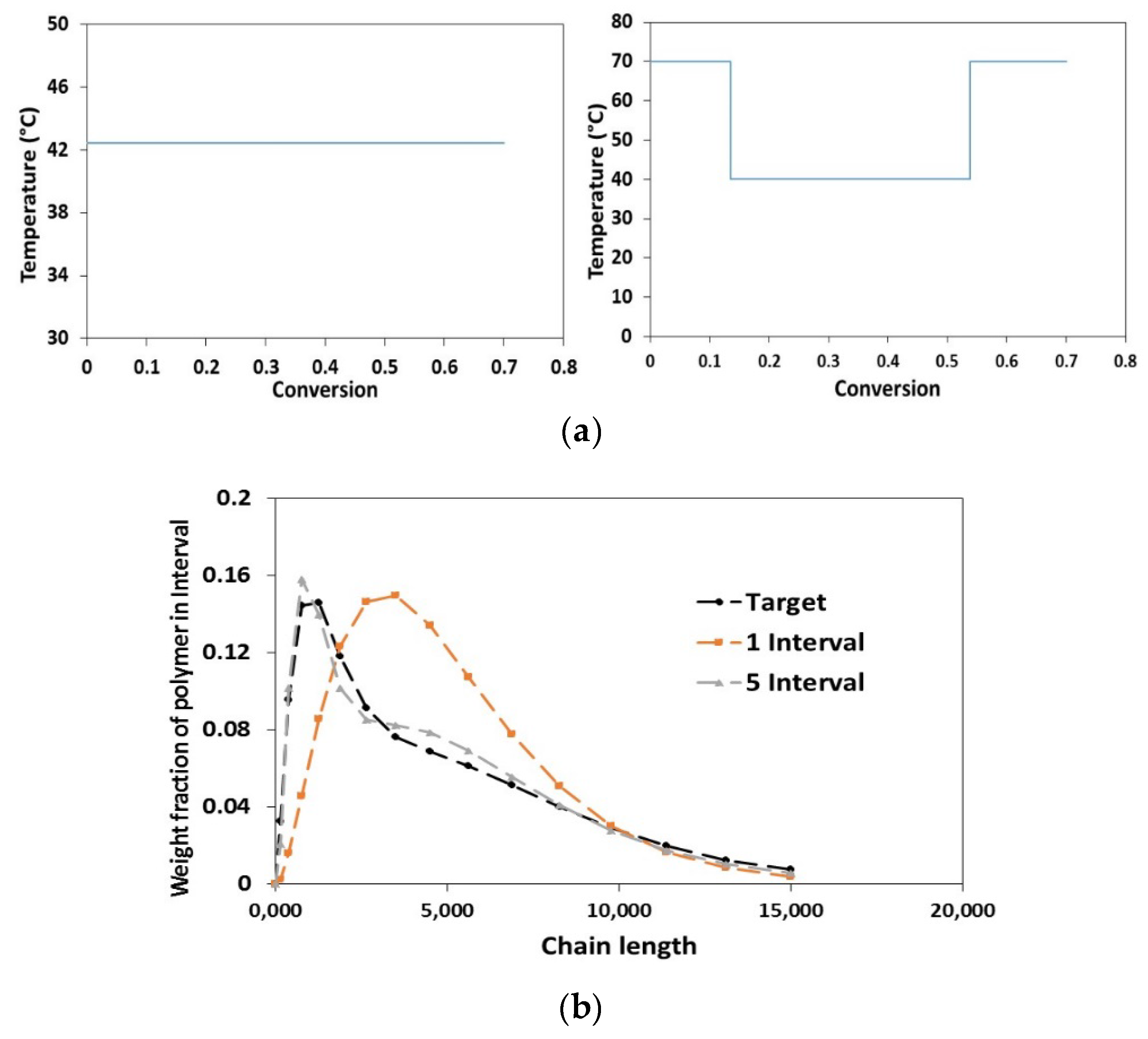
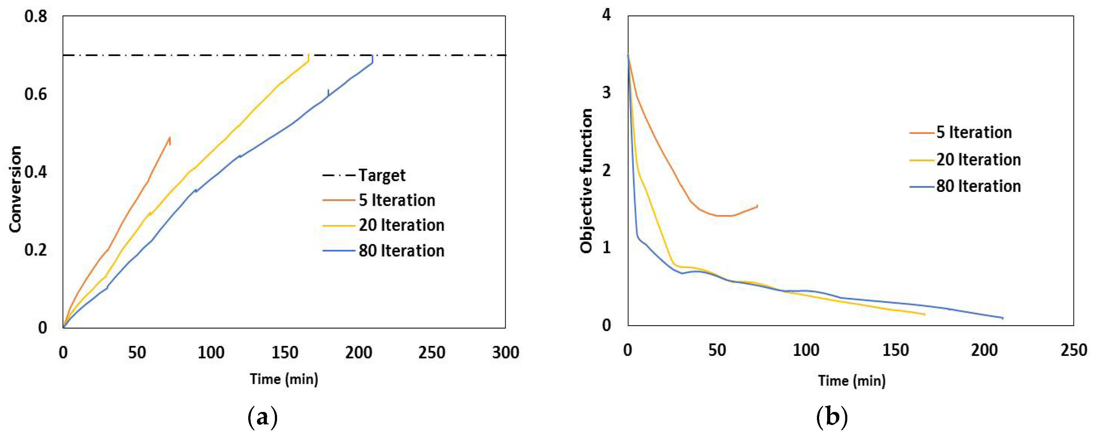
2.3. Dynamic Optimization
- Duration of each control interval and the values during the interval are selected by the optimizer
- Starting from the initial condition the dynamic system is solved in order to calculate the time-variation of the states of the system
- Based on the solution, the values of the objective function and its sensitivity to the control variables and also the constraints are determined.
- The optimizer revises the choices at the first step and the procedure is repeated until the convergence to the optimum condition is achieved.
3. Experimental System
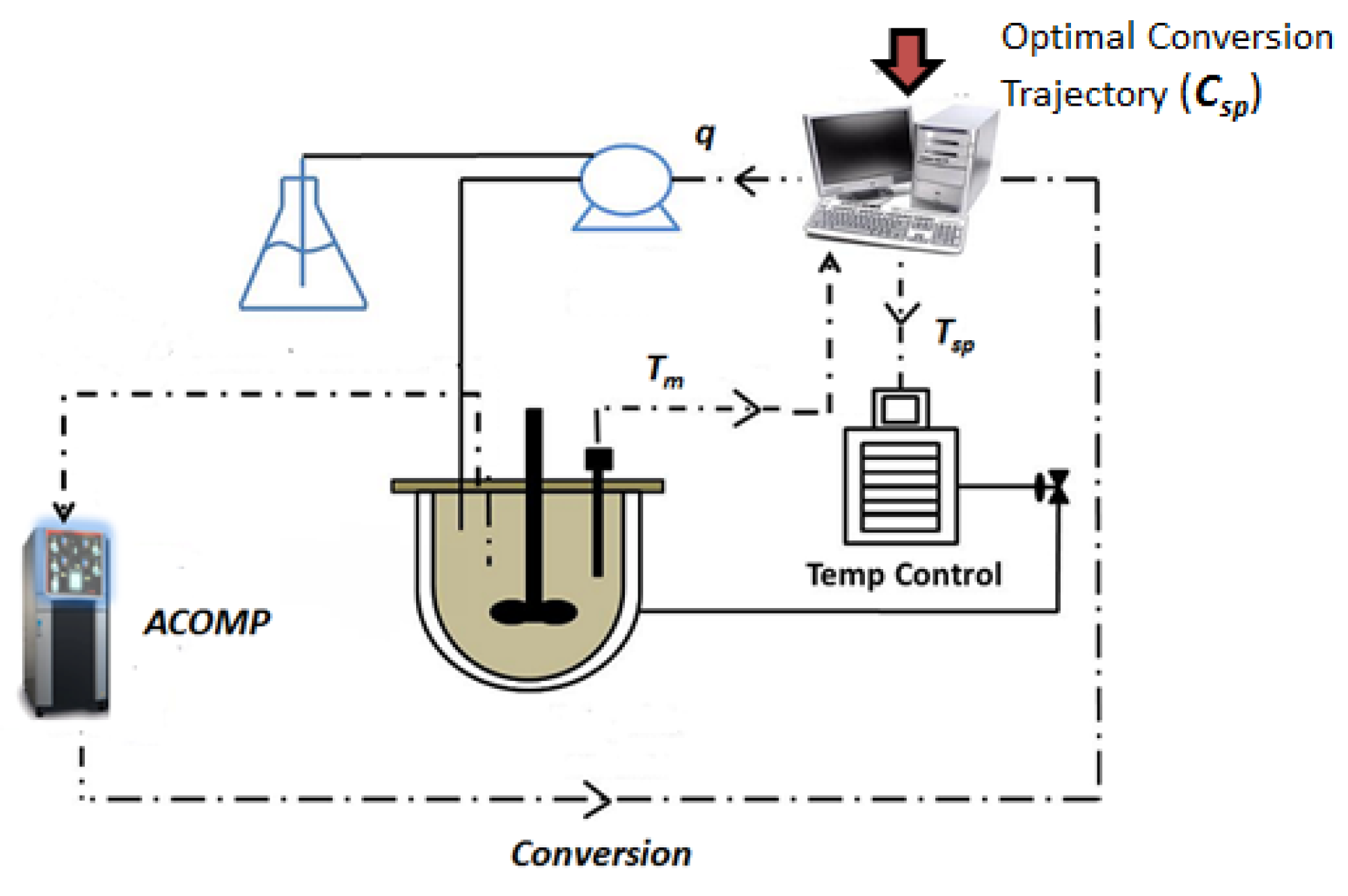
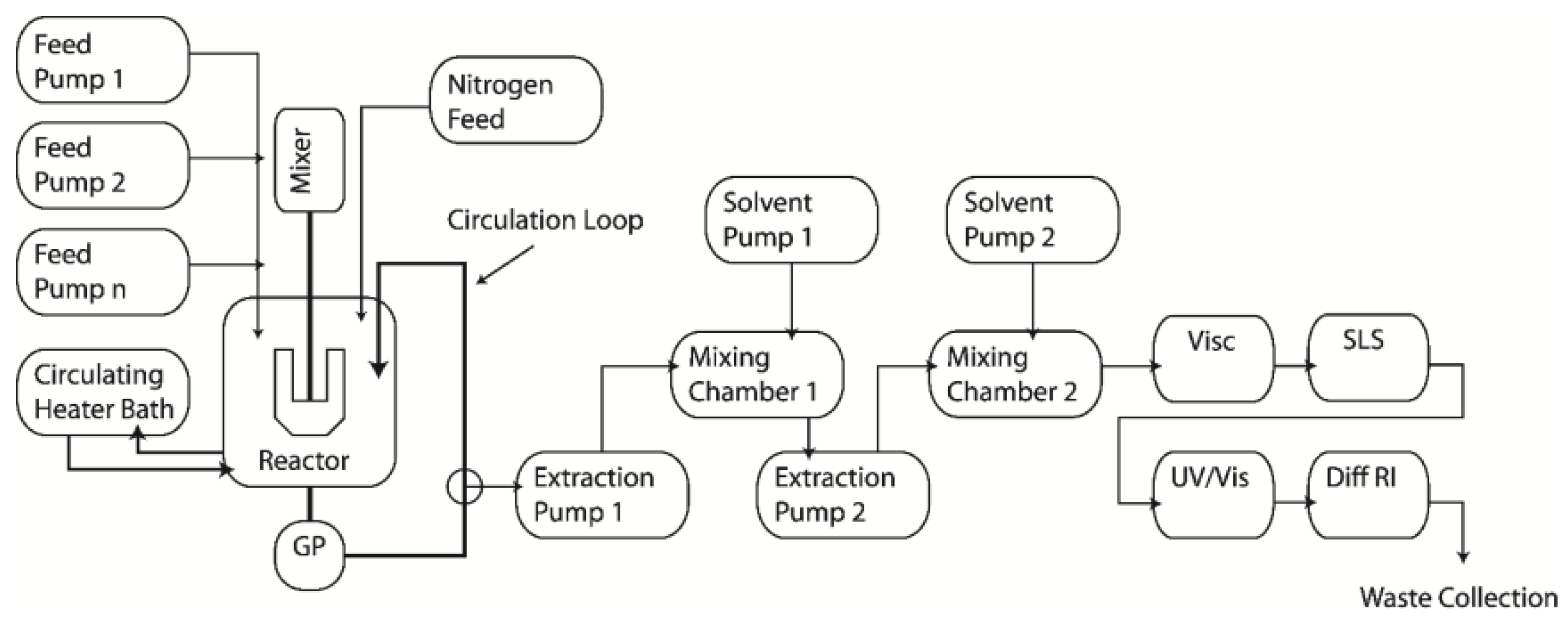
3.1. Experimental Apparatus—ACOMP System
3.2. Experimental Procedure
4. Results and Discussion
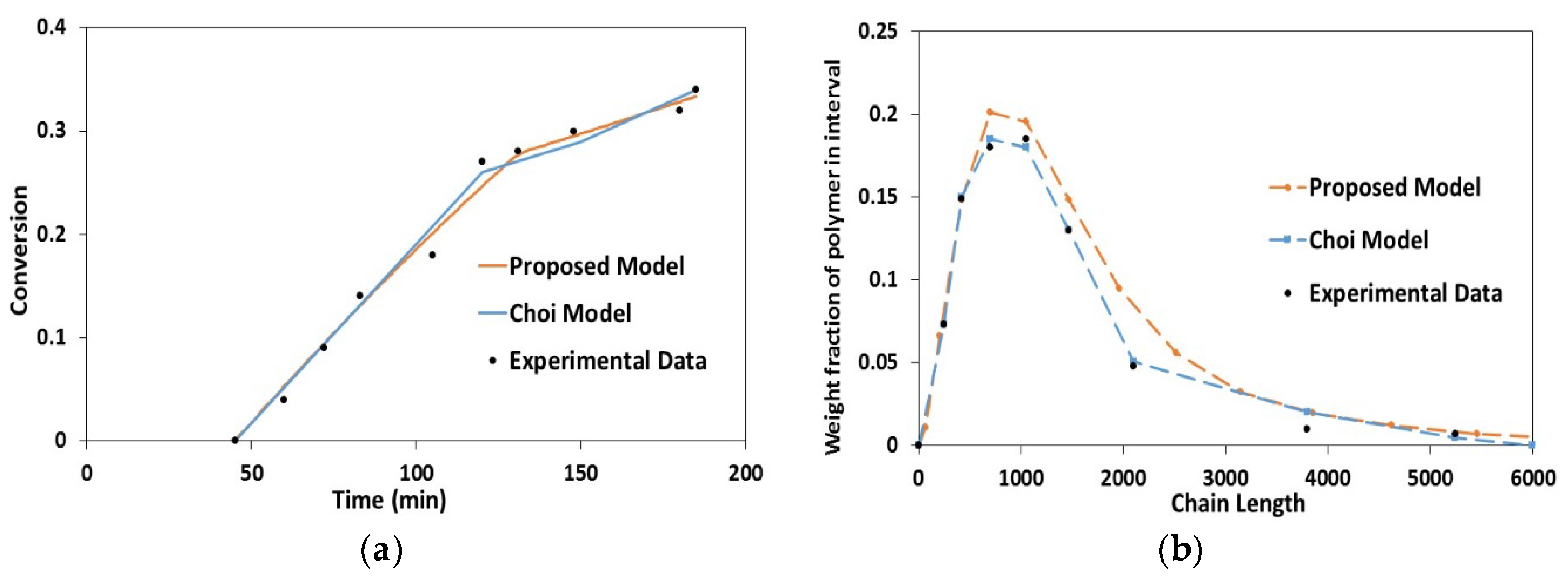
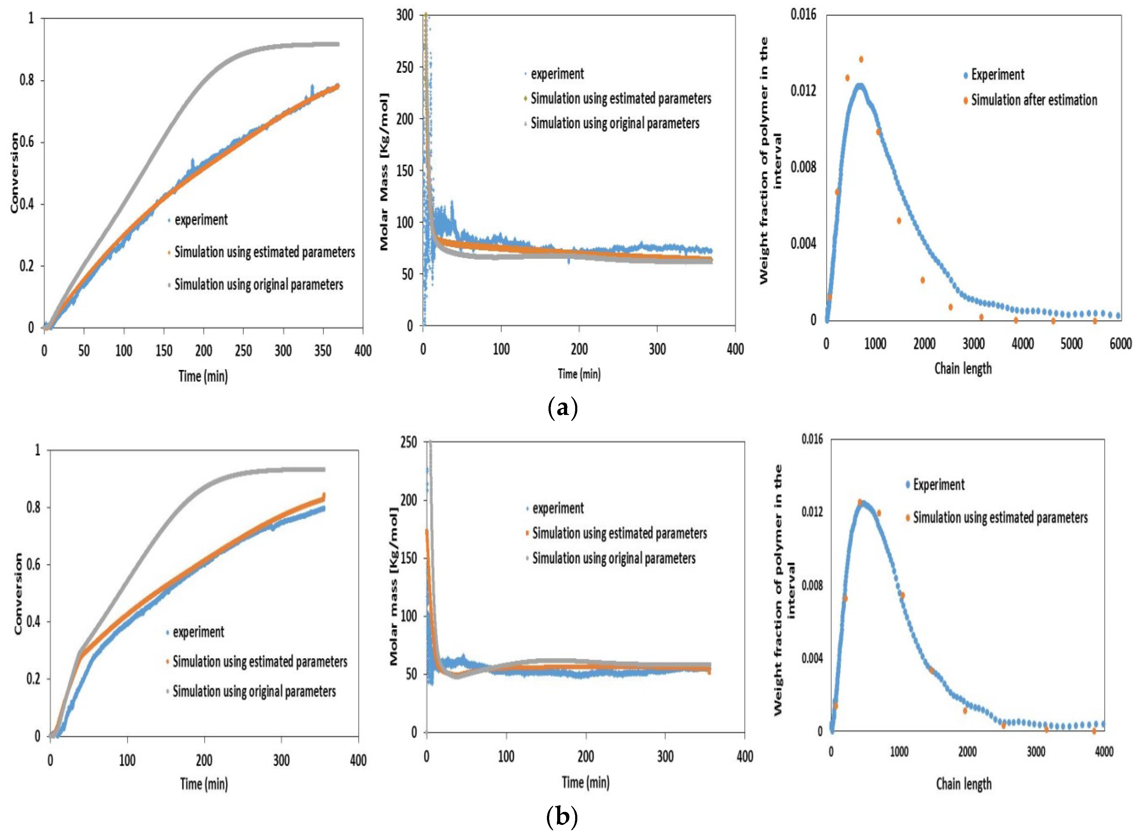
4.1. Validation Using Literature Data
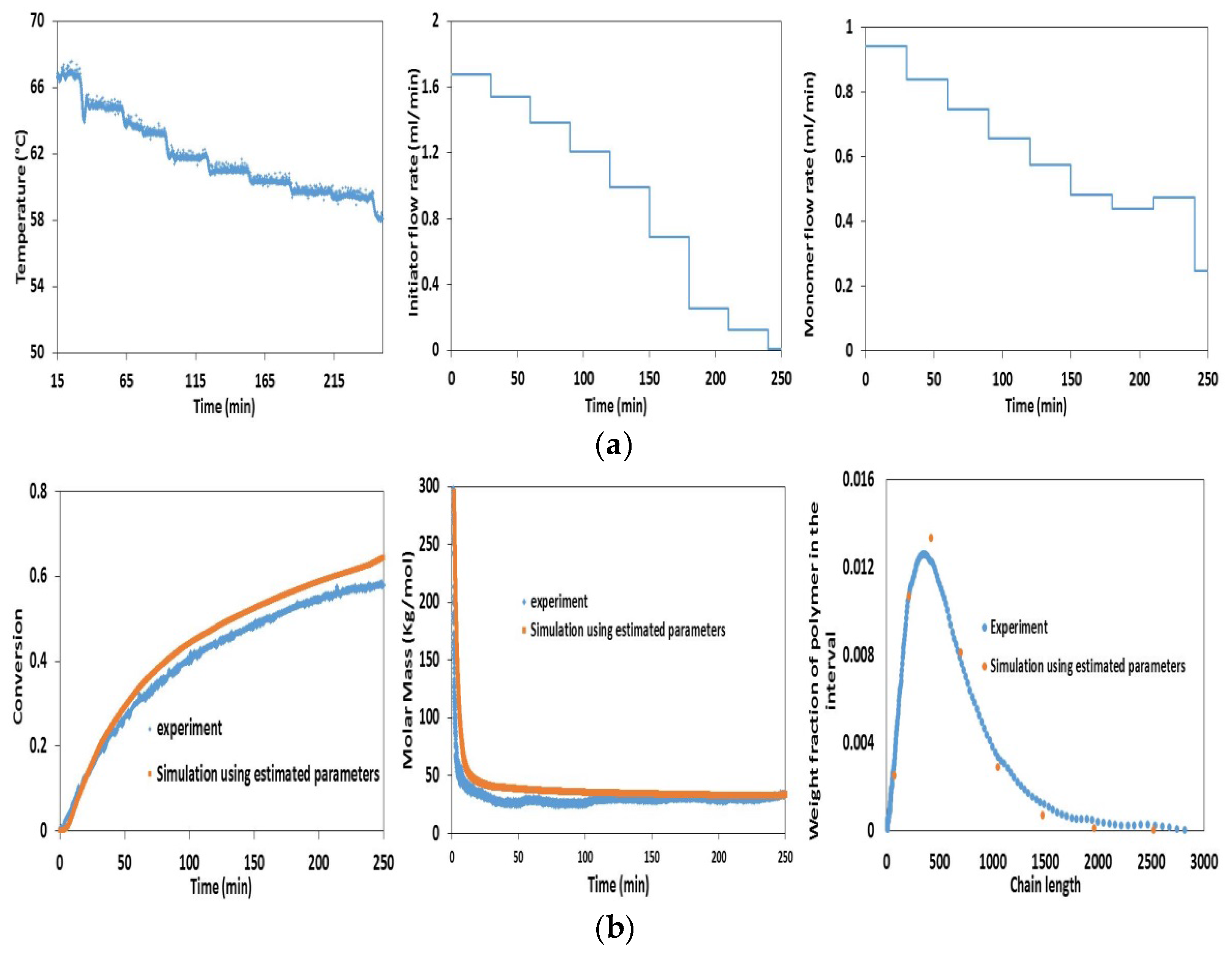
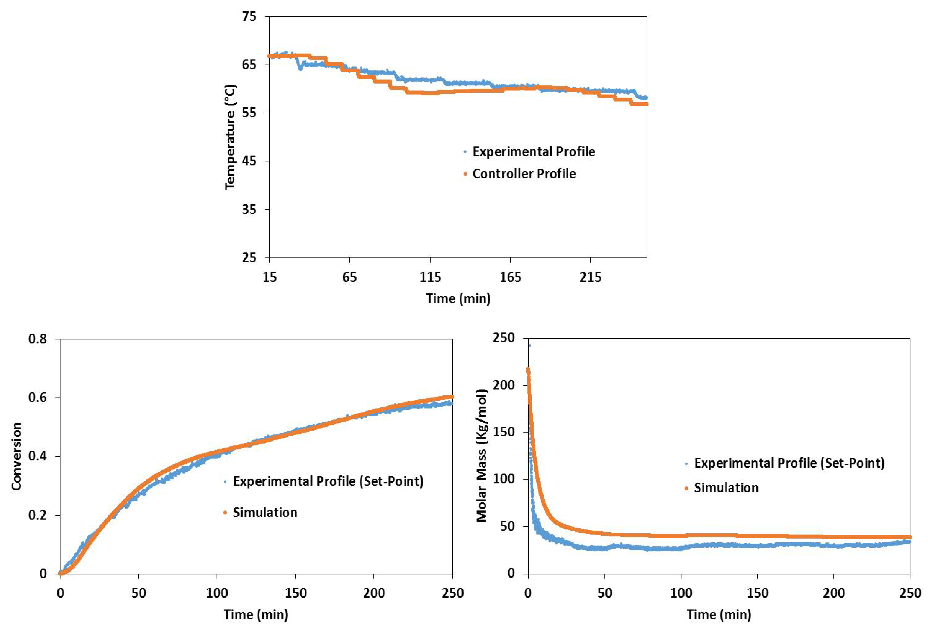
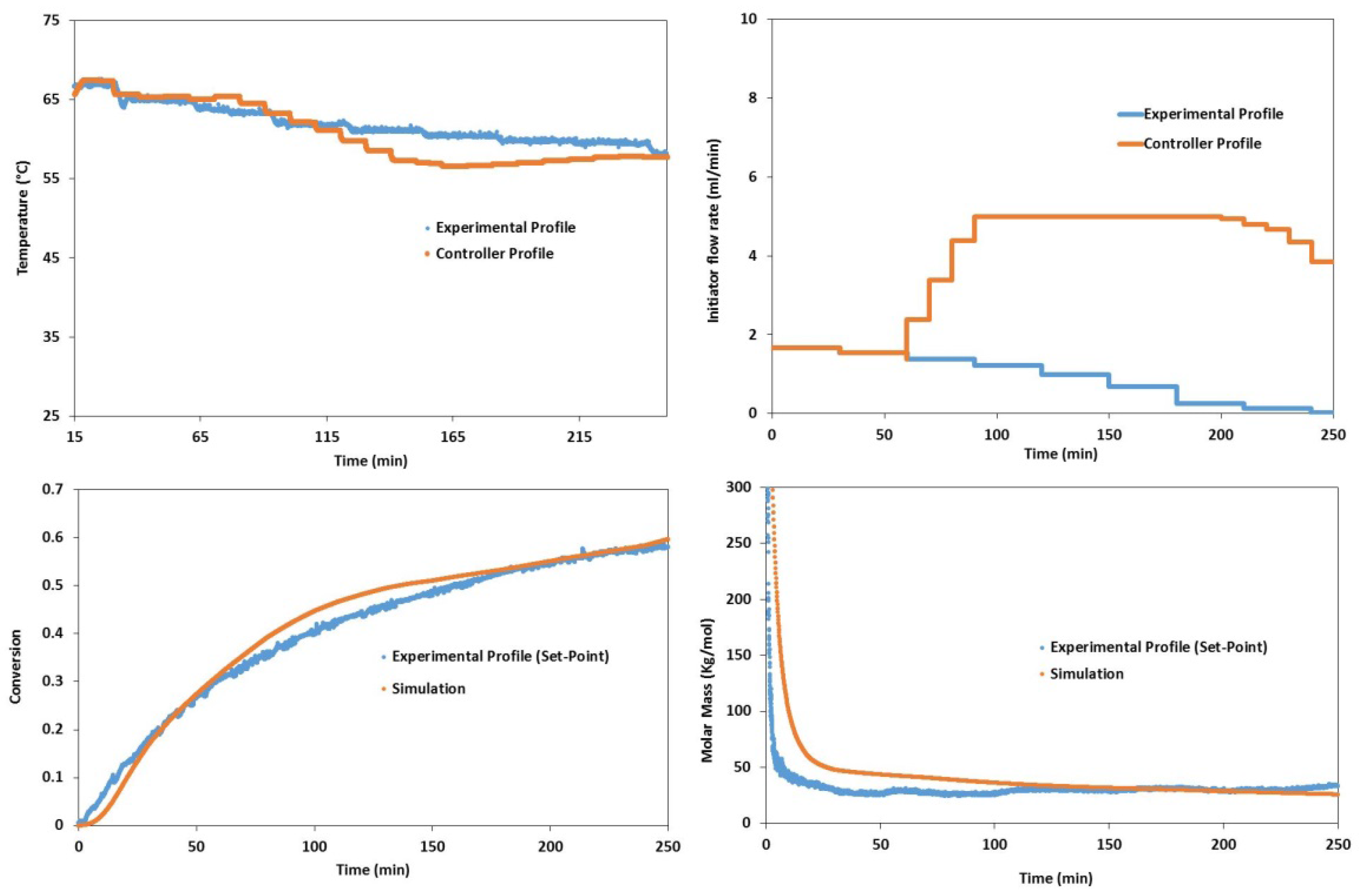
4.2. Experimental Validation for Batch and Semi-Batch Free Radical Polymerization of MMA Using Butyl Acetate as Solvent and AIBN Initiator
| Parameter | Description | Original Value | Estimated Value | Confidence Interval | 95% t-value | Standard Deviation | ||
|---|---|---|---|---|---|---|---|---|
| 90% | 95% | 99% | ||||||
| Ad | Decomposition (1/min) | 1.58 × 10¹⁵ | 1.37 × 10¹⁵ | 1.25 × 10¹⁴ | 1.49 × 10¹⁴ | 1.96 × 10¹⁴ | 9.19 | 7.60 × 10¹³ |
| Ap | Propagation (m3/mol∙min) | 4.2 × 10⁵ | 9 × 10⁵ | 5.23 × 10⁴ | 6.23 × 10⁴ | 8.20 × 10⁴ | 14.43 | 3.17 × 10⁴ |
| Atd | Termination [m3/mol∙min] | 1.06 × 10⁸ | 4.56 × 10⁸ | 5.97 × 10⁷ | 7.12 × 10⁷ | 9.37 × 10⁷ | 6.40 | 3.63 × 10⁷ |
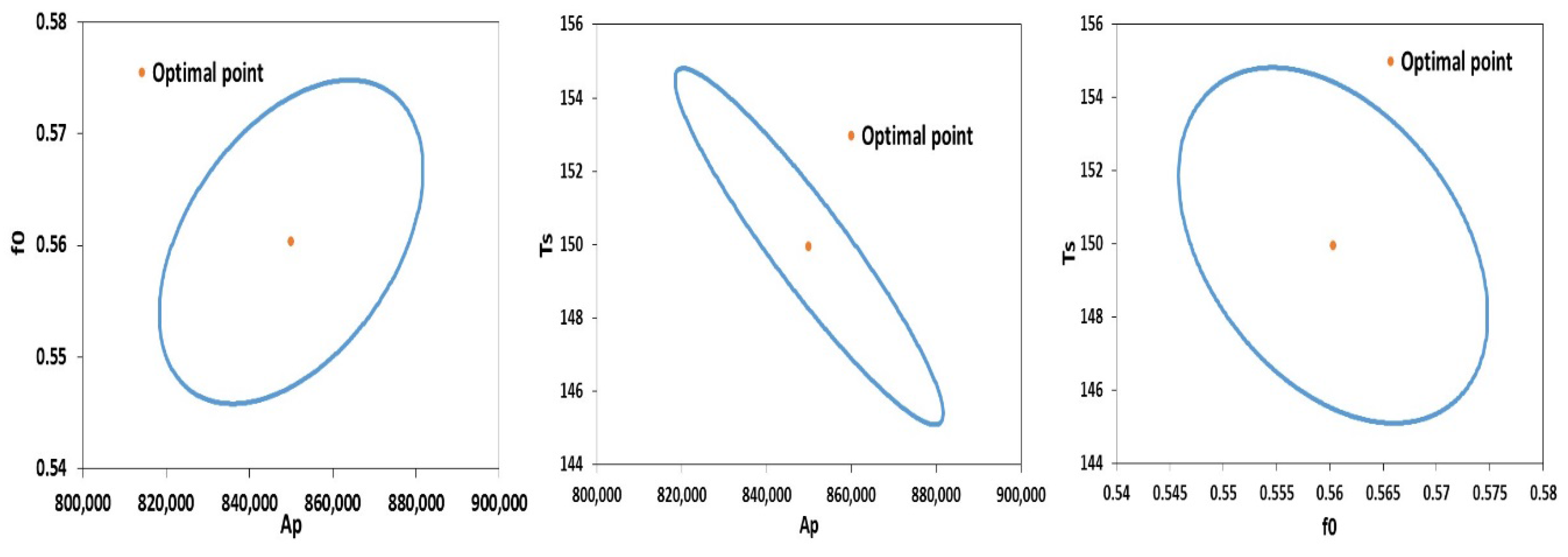
| f0 | Initial Initiator Efficiency | 0.58 | 0.57 | 0.048 | 0.057 | 0.076 | 9.84 | 0.029 |
| Ts | Solvent Transition Temperature (K) | 181 | 142.61 | 0.539 | 0.6431 | 0.84 | 221.7 | 0.327 |
| Estimated Parameters | Ad | Ap | At | f0 | Ts |
|---|---|---|---|---|---|
| Ad | 1 | - | - | - | - |
| Ap | 0.117 | 1 | - | - | - |
| At | 0.111 | 0.988 | 1 | - | - |
| f0 | –0.988 | 0.038 | 0.043 | 1 | - |
| Ts | 0.104 | 0.179 | 0.233 | –0.070 | 1 |

| Parameter | Description | Original Value | Estimated Value | Confidence Interval | 95% t-value | Standard Deviation | ||
|---|---|---|---|---|---|---|---|---|
| 90% | 95% | 99% | ||||||
| Ap | Propagation Rate (m3/mol∙min) | 3 × 10⁵ | 8.5 × 10⁵ | 2547 | 3035 | 3993 | 280.1 | 1546 |
| f0 | Initial Initiator Efficiency | 0.58 | 0.56 | 0.001166 | 0.0013 | 0.00182 | 403.2 | 0.00073 |
| Ts | Solvent Transition Temperature (K) | 142 | 149.94 | 0.3906 | 0.465 | 0.6123 | 322.2 | 0.237 |

| Variable | Value | Unit |
|---|---|---|
| Nm | 0.5 | mol |
| Ns | 0.5 | mol |
| Ni | 0.01 | mol |
| Fmax | 5 | mL/min |
| Fmin | 0 | mL/min |
| Tmax | 70 | °C |
| Tmin | 50 | °C |
| Vmax | 500 | mL |
| Vmin | 100 | mL |


5. Conclusions
Acknowledgments
Author Contributions
Conflicts of Interest
References
- Wu, T.; Yu, L.; Cao, Y.; Yang, F.; Xiang, M. Effect of molecular weight distribution on rheological, crystallization and mechanical properties of polyethylene-100 pipe resins. J. Polym. Res. 2013, 20, 1–10. [Google Scholar] [CrossRef]
- Schimmel, K.H.; Heinrich, G. The influence of the molecular-weight distribution of network chains on the mechanical-properties of polymer networks. Colloid Polym. Sci. 1991, 269, 1003–1012. [Google Scholar] [CrossRef]
- Malekmotiei, L.; Samadi-Dooki, A.; Voyiadjis, G.Z. Nanoindentation study of yielding and plasticity of poly(methyl methacrylate). Macromolecules 2015, 48, 5348–5357. [Google Scholar] [CrossRef]
- Guyot, A.; Guillot, J.; Pichot, C.; Guerrero, L.R. New design for production of constant composition co-polymers in emulsion polymerization—Comparison with co-polymers produced in batch. Abstr. Pap. Am. Chem. S 1980, 180, 131–ORPL. [Google Scholar]
- Dimitratos, J.; Georgakis, C.; Elaasser, M.S.; Klein, A. Dynamic modeling and state estimation for an emulsion copolymerization reactor. Comput. Chem. Eng. 1989, 13, 21–33. [Google Scholar] [CrossRef]
- Dimitratos, J.; Georgakis, C.; Elaasser, M.; Klein, A. An experimental-study of adaptive kalman filtering in emulsion copolymerization. Chem. Eng. Sci. 1991, 46, 3203–3218. [Google Scholar] [CrossRef]
- Hammouri, H.; McKenna, T.F.; Othman, S. Applications of nonlinear observers and control: Improving productivity and control of free radical solution copolymerization. Ind. Eng. Chem. Res. 1999, 38, 4815–4824. [Google Scholar] [CrossRef]
- Dochain, D.; Pauss, A. Online estimation of microbial specific growth-rates—An illustrative case-study. Can. J. Chem. Eng. 1988, 66, 626–631. [Google Scholar] [CrossRef]
- Kozub, D.J.; Macgregor, J.F. State estimation for semibatch polymerization reactors. Chem. Eng. Sci. 1992, 47, 1047–1062. [Google Scholar] [CrossRef]
- Mutha, R.K.; Cluett, W.R.; Penlidis, A. On-line nonlinear model-based estimation and control of a polymer reactor. Aiche. J. 1997, 43, 3042–3058. [Google Scholar] [CrossRef]
- Mutha, R.K.; Cluett, W.R.; Penlidis, A. A new multirate-measurement-based estimator: Emulsion copolymerization batch reactor case study. Ind. Eng. Chem. Res. 1997, 36, 1036–1047. [Google Scholar] [CrossRef]
- Kravaris, C.; Wright, R.A.; Carrier, J.F. Nonlinear controllers for trajectory tracking in batch processes. Comput. Chem. Eng. 1989, 13, 73–82. [Google Scholar] [CrossRef]
- Alhamad, B.; Romagnoli, J.A.; Gomes, V.G. On-line multi-variable predictive control of molar mass and particle size distributions in free-radical emulsion copolymerization. Chem. Eng. Sci. 2005, 60, 6596–6606. [Google Scholar] [CrossRef]
- Garcia, C.E.; Morari, M. Internal model control.1. A unifying review and some new results. Ind. Eng. Chem. Proc. Dd. 1982, 21, 308–323. [Google Scholar] [CrossRef]
- Park, M.J.; Rhee, H.K. Control of copolymer properties in a semibatch methyl methacrylate/methyl acrylate copolymerization reactor by using a learning-based nonlinear model predictive controller. Ind. Eng. Chem. Res. 2004, 43, 2736–2746. [Google Scholar] [CrossRef]
- Gattu, G.; Zafiriou, E. Nonlinear quadratic dynamic matrix control with state estimation. Ind. Eng. Chem. Res. 1992, 31, 1096–1104. [Google Scholar] [CrossRef]
- Lee, J.H.; Ricker, N.L. Extended kalman filter based nonlinear model-predictive control. Ind. Eng. Chem. Res. 1994, 33, 1530–1541. [Google Scholar] [CrossRef]
- Henson, M.A. Nonlinear model predictive control: Current status and future directions. Comput. Chem. Eng. 1998, 23, 187–202. [Google Scholar] [CrossRef]
- Schork, F.J.; Deshpande, P.B.; Leffew, W.K. Control of polymerization reactors; CRC Press: Boca Raton, FL, USA, 1993; pp. 101–104. [Google Scholar]
- Crowley, T.J.; Choi, K.Y. Experimental studies on optimal molecular weight distribution control in a batch-free radical polymerization process. Chem. Eng. Sci. 1998, 53, 2769–2790. [Google Scholar] [CrossRef]
- Ellis, M.F.; Taylor, T.W.; Jensen, K.F. Online molecular-weight distribution estimation and control in batch polymerization. Aiche. J. 1994, 40, 445–462. [Google Scholar] [CrossRef]
- Congalidis, J.P.; Richards, J.R.; Ray, W.H. Feedforward and feedback-control of a solution copolymerization reactor. Aiche. J. 1989, 35, 891–907. [Google Scholar] [CrossRef]
- Adebekun, D.K.; Schork, F.J. Continuous solution polymerization reactor control 2. Estimation and nonlinear reference control during methyl-methacrylate polymerization. Ind. Eng. Chem. Res. 1989, 28, 1846–1861. [Google Scholar] [CrossRef]
- Florenzano, F.H.; Strelitzki, R.; Reed, W.F. Absolute, on-line monitoring of molar mass during polymerization reactions. Macromolecules 1998, 31, 7226–7238. [Google Scholar] [CrossRef]
- Giz, A.; Catalgil-Giz, H.; Alb, A.; Brousseau, J.L.; Reed, W.F. Kinetics and mechanisms of acrylamide polymerization from absolute, online monitoring of polymerization reaction. Macromolecules 2001, 34, 1180–1191. [Google Scholar] [CrossRef]
- Reed, W.F. Automated continuous online monitoring of polymerization reactions (acomp) and related techniques. Anal. Chem. 2013. [Google Scholar] [CrossRef]
- Baillagou, P.E.; Soong, D.S. Major factors contributing to the nonlinear kinetics of free-radical polymerization. Chem. Eng. Sci. 1985, 40, 75–86. [Google Scholar] [CrossRef]
- Pinto, J.C.; Ray, W.H. The dynamic behavior of continuous solution polymerization reactors 7. Experimental-study of a copolymerization reactor. Chem. Eng. Sci. 1995, 50, 715–736. [Google Scholar] [CrossRef]
- Ray, W.H. Mathematical modeling of polymerization reactors. J. Macromol. Sci. R M C 1972, 8, 1–56. [Google Scholar] [CrossRef]
- Crowley, T.J.; Choi, K.Y. Calculation of molecular weight distribution from molecular weight moments in free radical polymerization. Ind. Eng. Chem. Res. 1997, 36, 1419–1423. [Google Scholar] [CrossRef]
- Crowley, T.J.; Choi, K.Y. Optimal control of molecular weight distribution in a batch free radical polymerization process. Ind. Eng. Chem. Res. 1997, 36, 3676–3684. [Google Scholar] [CrossRef]
- Ross, R.T.; Laurence, R.L. Gel effect and free volume in the bulk polymerization of methyl methacrylate. Aiche. J. 1976, 72, 74–79. [Google Scholar]
- Fan, S.; Gretton-Watson, S.P.; Steinke, J.H.G.; Alpay, E. Polymerisation of methyl methacrylate in a pilot-scale tubular reactor: Modelling and experimental studies. Chem. Eng. Sci. 2003, 58, 2479–2490. [Google Scholar] [CrossRef]
- Li, R.J.; Henson, M.A.; Kurtz, M.J. Selection of model parameters for off-line parameter estimation. IEEE T Contr. Syst. T 2004, 12, 402–412. [Google Scholar] [CrossRef]
- Nowee, S.M.; Abbas, A.; Romagnoli, J.A. Optimization in seeded cooling crystallization: A parameter estimation and dynamic optimization study. Chem. Eng. Process. 2007, 46, 1096–1106. [Google Scholar] [CrossRef]
© 2016 by the authors; licensee MDPI, Basel, Switzerland. This article is an open access article distributed under the terms and conditions of the Creative Commons by Attribution (CC-BY) license (http://creativecommons.org/licenses/by/4.0/).
Share and Cite
Ghadipasha, N.; Geraili, A.; Romagnoli, J.A.; Castor, C.A., Jr.; Drenski, M.F.; Reed, W.F. Combining On-Line Characterization Tools with Modern Software Environments for Optimal Operation of Polymerization Processes. Processes 2016, 4, 5. https://doi.org/10.3390/pr4010005
Ghadipasha N, Geraili A, Romagnoli JA, Castor CA Jr., Drenski MF, Reed WF. Combining On-Line Characterization Tools with Modern Software Environments for Optimal Operation of Polymerization Processes. Processes. 2016; 4(1):5. https://doi.org/10.3390/pr4010005
Chicago/Turabian StyleGhadipasha, Navid, Aryan Geraili, Jose A. Romagnoli, Carlos A. Castor, Jr., Michael F. Drenski, and Wayne F. Reed. 2016. "Combining On-Line Characterization Tools with Modern Software Environments for Optimal Operation of Polymerization Processes" Processes 4, no. 1: 5. https://doi.org/10.3390/pr4010005