Methods and Tools for Robust Optimal Control of Batch Chromatographic Separation Processes

Abstract

This contribution concerns the development of generic methods and tools for robust optimal control of high-pressure liquid chromatographic separation processes. The proposed methodology exploits a deterministic robust formulation, that employs a linearization of the uncertainty set, based on Lyapunov differential equations to generate optimal elution trajectories in the presence of uncertainty. Computational tractability is obtained by casting the robust counterpart problem in the framework of bilevel optimal control where the upper level concerns forward simulation of the Lyapunov differential equation, and the nominal open-loop optimal control problem augmented with the robustified target component purity inequality constraint margin is considered in the lower level. The lower-level open-loop optimal control problem, constrained by spatially discretized partial differential equations, is transcribed into a finite dimensional nonlinear program using direct collocation, which is then solved by a primal-dual interior point method. The advantages of the robustification strategy are highlighted through the solution of a challenging ternary complex mixture separation problem for a hydrophobic interaction chromatography system. The study shows that penalizing the changes in the zero-order hold control gives optimal solutions with low sensitivity to uncertainty. A key result is that the robustified general elution trajectories outperformed the conventional linear trajectories both in terms of recovery yield and robustness.

1. Introduction

Isolation of a high-purity target component from a multicomponent mixture is of significant importance in the pharmaceutical and biochemical industries [1]. In the clinical or commercial-scale manufacturing of human therapeutic proteins, high-pressure liquid chromatography (HPLC) is an essential process operation to achieve the high purity requirements for biopharmaceutical drugs [2,3]. Due to inflexibility in the conventional regulatory paradigm, applying process operational changes to an approved process design in the biopharmaceutical community has been historically prohibited without filing for a new approval [1]. The United States Food and Drug Administration (US FDA) has published a series of new guidelines to promote flexibility for innovation while appropriately managing variability in the process performance attributes for continual improvement via process analytical technology (PAT) and quality-by-design (QbD) principles [4,5]. QbD promotes improved process understanding during process and product development and building quality in the design instead of testing for quality. This can be achieved via correlative, causal, or mechanistic knowledge and at the highest level via first principle models. Hence, PAT has been gaining a lot of momentum in the biopharmaceutical community due to the potential for continuous real time quality assurance resulting in improved operational control and compliance [6].

In the QbD approach, critical quality attributes (CQA) of pharmaceutical products are defined that assure desired clinical performance, and then a manufacturing process is designed to consistently meet these product attributes, thus assuring product quality [7]. Process characterization is conducted to identify the impact of process parameters on the products CQA’s [8], which is then used to define a process design space. A design space is defined as “the multidimensional combination and interaction of input variables and process parameters that have been demonstrated to provide an assurance of product quality” [9]. Acceptable ranges for process parameters and input variables are documented in the regulatory filing, and working within these ranges is not deemed to be a change from normal operating conditions. The expected benefit of the QbD approach is an increase in the assurance of product quality, and in turn, the FDA will allow manufacturers greater flexibility to operate with lower regulatory burden, enabling continuous process improvement, as well as greater robustness [10].

The current approach to process characterization within the QbD framework is concerned with validating that the defined design space can cope with the process variability experienced during normal operation [10]. In this context, the FDA guidance encourages the application of mechanistic models to improve process understanding, based on fundamental knowledge of the underlying physico-chemical phenomena correlating the nonlinear interdependence of process parameters and inputs to the resulting value of the CQA’s. Model-based approaches to sensitivity and robustness analysis have been successfully applied to a diversity of chromatographic separations, see e.g., Mota et al. [11], Degerman et al. [12], Westerberg et al. [13], Borg et al. [14] and the references cited therein. The aforementioned robustness assessment investigations have exclusively been founded on stochastic methodologies, in which inherent process parameters and inputs have been randomly generated from a uniform or a truncated normal distribution, to determine the magnitude of variability of the CQA’s. The result is a probability density distribution of the output, which can be used to determine the risk of batch failure and the process capability as well as to identify inputs that can be used to design a control strategy. In this context, the main objective of this study is to exploit recent advances in deterministic robustness strategies in conjunction with open-loop optimal control.

1.1. Solvent Composition Trajectory Elution Strategies

Solvent composition trajectory elution is widely applied in both analytical and preparative chromatography, and refers to a continuous change in the mobile phase during separation [15]. By this means, improved resolution of highly complex sample mixtures can be obtained in a much shorter time than could be expected in isocratic elution conditions. Reproducible selectivity in chromatographic separation of closely related product impurities requires optimized elution mode and fractionation interval endpoints [16]. The current state-of-the-art methodology for optimization of HPLC separations has been limited to linear [17,18], concave/convex [19] and step elution trajectories [20]. A novel open-loop optimal control strategy for simultaneous optimization of general elution trajectories and target component fractionating decisions was recently developed by Holmqvist and Magnusson [21], Holmqvist et al. [22]. The present investigation is a direct continuation of these studies and the overall objective is to extend the open-loop optimal control strategy with a robust worst-case formulation and benchmark the robustness of general elution trajectories, with respect to target component purity, with that of the conventional linear trajectories.

In the context of the QbD framework, this implies relating the impact of a critical process parameter (CPP) to the difference between the quality requirement and the CQA at the nominal operating point, i.e., assess the level of reduction in the robustness safety margin. A CPP is formally defined as “a process parameter whose variability has an impact on a critical quality attribute and, therefore, should be monitored or controlled to ensure the process produces the desired quality” [23]. A quantitative value of the sensitivity of the CQA with respect to CPPs can be obtained by scaling the discrepancy between the CQA value at the nominal operating point and the requirement by perturbation of the CPP values of $1.0$ standard deviation in the direction that gives the worst-case value of the QCA [13]:

$$\left|{\displaystyle \frac{QC{A}_{\mathrm{nom}}-QC{A}_{\pm \sigma }}{QC{A}_{\mathrm{nom}}-QC{A}_{\mathrm{req}}}}\right|.$$

The higher the value, the more likely the parameter is to cause batch failure. Thus, it is noteworthy that the open-loop controlled system targeting the captured amount of the target component with respect to the fractionating interval endpoints yields that the inequality constraint imposed on target component purity is active, i.e., the resulting purity equals its lower requirement [16]. Consequently, there is no inherent safety margin incorporated in the open-loop optimal control problem and to surmount this shortcoming calls for the formulation of a robust counterpart problem [24].

1.2. PDE-Constrained Dynamic Optimization

In this study, the realistic multi-component system dynamics required for analysis were generated by numerical solution of the reaction–dispersive model [25]. This model is governed by a set of mass-balance partial differential equations (PDEs), with a modified Langmuir isotherm and experimentally validated kinetics. In this regard, the advantages of this robust optimal control framework are highlighted through the solution of a challenging ternary mixture separation problem, with human insulin (insulin aspart, desB30 insulin and insulin methyl ester) and the intermediately eluting component as the target, for a hydrophobic interaction chromatography (HIC) [26,27] system.

The proposed model-based methodology for robust optimal control implies formulating and solving a large-scale dynamic optimization problem (DOP) constrained by PDEs [28]. Optimal design, optimal control, and parameter estimation of systems governed by PDE give rise to a class of problems known as PDE-constrained optimization [29,30]. The size and complexity of the discretized PDEs often pose significant challenges for contemporary optimization methods. There exists two generic direct methods to transform the infinite DOP into a finite dimensional nonlinear program (NLP); sequential and simultaneous [31,32]. Optimization studies of HPLC separations carried out in the literature have exclusively been using sequential methods, where the system dynamics constraint is handled by embedded numerical integrators, and where the PDEs are approximated using the method-of-lines [33,34] and Galerkin finite element or finite volume methods. Both gradient-based NLP solvers (e.g., sequential quadratic programming and interior-point method) [35,36,37] and those based on trajectory free heuristic approaches (e.g., generic algorithms and simulated annealing) [18,38,39] have been used successfully. The proposed methodology in this paper is based on a developed simultaneous method where both the control and state variables are fully discretized in the temporal domain using orthogonal collocations on finite elements [31]. In order to reduce the size of the resulting NLP, the PDE system was approximated using an adaptive, high order finite volume weighted essentially non-oscillatory (WENO) scheme [40,41,42]. The NLP is subsequently solved using the primal-dual interior point method IPOPT [43] and algorithmic differentiation (AD) techniques [44].

Jacobians are required by gradient-based NLP algorithms and simulation. Access to accurate Jacobians often improves the performance and robustness of algorithms, and in addition, efficient implementation of Jacobian computations can reduce the over-all execution time. In the context of HPLC system modelling, Püttmann et al. [45] compared the accuracy of Jacobians, with respect to an intrinsic model parameter, computed using first-order finite differences (FD) and AD. It was shown in that study the AD approach outperformed the FD approach in terms of both accuracy and over-all execution time for realistically sized chromatography models when computing forward sensitivities of the DAE system, i.e., the linearization of the original system with respect to an intrinsic model parameter. The AD approach in [45] is extended in this paper to include computations of Hessians required by the NLP solver but also addresses the construction of metrics required in the robust counterpart formulation.

1.3. Nonlinear Robust Optimization of Uncertain Dynamic Systems

As outlined above, uncertainty propagation of CPPs through nonlinear model equations is reflected in terms of QCAs (e.g., constraints and objectives). Methodologies developed to cope with the complexity of optimization problems under uncertainty can be categorized into stochastic programming, probabilistic (chance-constraint) programming and fuzzy programming [46]. The stochastic programming formulations assume that the probability distributions governing the uncertain parameters are available or can be estimated from the existing data. Here, reliability requires feasibility for all the outcomes of uncertain parameters, whereas chance-constrained programming requires feasibility of solutions with at least some probability specified on constraints having uncertain parameters. The main advantage of the chance-constrained programming technique is the emergence of a deterministic equivalent problem [47]. In the deterministic formulations, the nature of the uncertainty is assumed to be bounded to a prespecified set, and reliability requires that all constraints are satisfied in all possible worst case situations. In any case, including more robustness gives rise to a lower performance, and hence, robustness can be interpreted as an additional and conflicting objective [48].

In this study we concentrate on the case that the dynamic system governed by PDEs is affected by a time variant input with uncertainties. To efficiently and accurately generate optimal elution trajectories in the presence of uncertainty we consider a deterministic robust formulation, that employs a linearization of the uncertainty set, proposed in the article series by Logist et al. [49], Houska and Diehl [50], Houska et al. [51]. The main objective is to robustly regard inequality state constraints. For this aim, the proposed methodology utilizes Lyapunov differential equations to compute variance-covariance matrix functions and facilitates the tractable robust counterpart formulation for optimal control problems.

1.4. Aim and Scope

External process disturbances are inevitably present and the robustness of the open-loop controlled system with respect to CPP uncertainties, e.g., guaranteeing that QCA requirements are not violated, is of the highest importance in biopharmaceutical process industry. It is, however, noteworthy that there is a drastic increase in computational complexity while moving from the nominal problem to its robust counterpart. The main contribution of this paper is therefore to establish a methodology and a computationally efficient framework for robust optimal control yielding robust general elution trajectories, with respect to target component purity, for batch chromatographic separation processes. The study presented here had three main objectives:

i)

To formulate a nominal open-loop optimal control problem and its robust counterpart, including penalty on the difference on the zero-order hold control discretization, to find optimal control trajectories that remain feasible for all perturbations from the uncertainty set.

ii)

To develop a numerically efficient framework for simulation of a Lyapunov differential equation, enabling the computation of the robustified inequality constraint margin in the counterpart problem.

iii)

To assess the robustness of general elution trajectories, for both batch elution and cyclic-steady-state operation, and to benchmark with that of the conventional liner trajectories.

1.5. Outline of the Paper

The remainder of this paper is structured as follows: Section 2 presents the HPLC separation system. Section 3 outlines the process model and the spatial discretization scheme. Section 4 describes the open-loop and robust counterpart problem formulation. Section 5 outlines the methods and tools for dynamic simulation and optimization. Section 6 presents the primary results, and Section 7 contains concluding remarks and perspectives for future research.

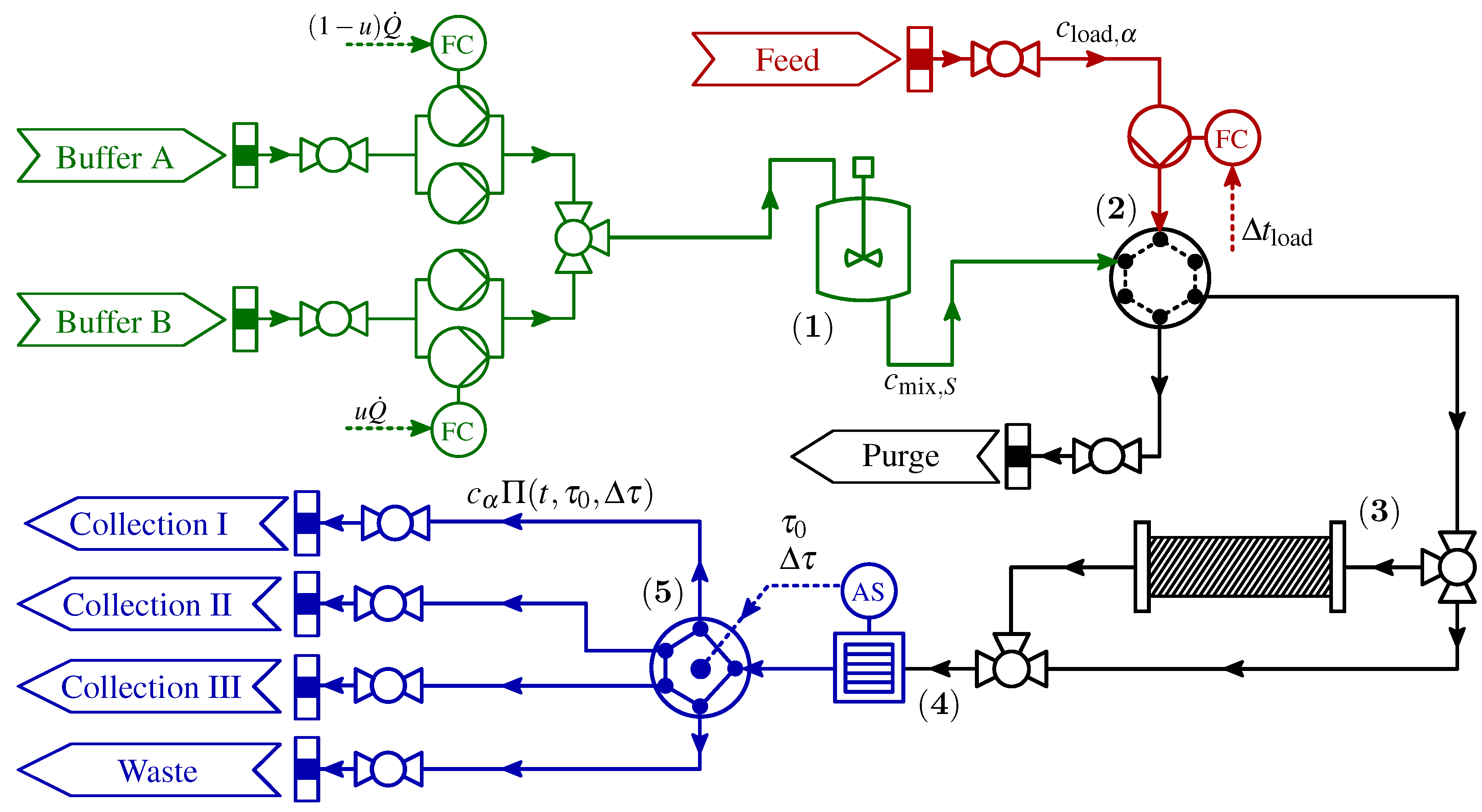
2. Process Description

The HPLC separation system operated in batch mode is characterized by subsequent pulse injections of the sample mixture and relies on pumps to pass a pressurized liquid solvent containing the sample mixture through a column packed with a solid adsorbent material [52]. A simplified P&ID of a standard HPLC system under consideration is illustrated in Figure 1. The system facilitates implementation of zero-order hold elution trajectories, u, through control of the volume fraction of buffers with different solvent strengths [53]. The resulting time-variant mobile phase modifier concentration, $c_{\mathrm{mix},S}$, is obtained in the mixing unit and enters the separation column with the system volumetric flow rate $\dot{Q}$. Moreover, the feed, with concentration $c_{\mathrm{load},\alpha }$ and $\alpha \in \{A,B,C\}$, is injected as a rectangular pulse with duration $\Delta t_{\mathrm{load}}$ via a multiport valve. The eluting concentration trajectory is analyzed with a UV detector at the column outlet [54], and a fractionating valve separates the mixture into its components [36]. The fractionating interval manipulating variables $[{\tau }_0,\Delta \tau ]$ govern the maximum recovery yield while still fulfilling the constraint imposed on purity of the target component fraction [16]. The time-invariant operating parameters $[\dot{Q},c_{\mathrm{load},\alpha },\Delta t_{\mathrm{load}}]$ are summarized in Table 1 and the optimal control problem optimization variables include the piecewise constant controls of the parameterized elution trajectory, $u_i$ and $\forall i\in [1..N_u]$, and $[{\tau }_0,\Delta \tau ]$.

Figure 1. Simplified P&ID of the HPLC system. Elementary system component description: (1) buffer mixing unit, (2) high-pressure switching valve unit, (3) HPLC separation column, (4) UV detector, and (5) fractionating valve.

Figure 1. Simplified P&ID of the HPLC system. Elementary system component description: (1) buffer mixing unit, (2) high-pressure switching valve unit, (3) HPLC separation column, (4) UV detector, and (5) fractionating valve.

Table 1. HPLC system component design parameters and HIC column specifics. The adsorption capacity and the self-association parameters listed are equal for all insulin variants $\alpha \in \{A,B,C\}$.

Parameter	Description	Value	Unit
$\dot{Q}$	volumetric flow rate	$6.0\times {10}^{-5}$	${\mathrm{m}}^3·{\mathrm{s}}^{-1}$
$\Delta t_{\mathrm{load}}$	sample load duration	$1.0\times {10}^{-2}$	s
$V_{\mathrm{mix}}$	buffer mixing unit volume	$2.0\times {10}^{-7}$	${\mathrm{m}}^3$
$L_c$	column length	$1.0\times {10}^{-1}$	m
$D_c$	column diameter	$1.0\times {10}^{-2}$	m
$D_p$	particle diameter	$3.5\times {10}^{-5}$	m
${\epsilon }_c$	interstitial porosity of the column	$3.26\times {10}^{-1}$	−
${\epsilon }_p$	apparent particle porosity	$7.54\times {10}^{-1}$	−
${\epsilon }_t$	total porosity of the column	${\epsilon }_c+(1-{\epsilon }_c){\epsilon }_p$	−
${𝒟}_{\mathrm{app}}$a	apparent dispersion coefficient	$\left(v_{\mathrm{int}}{D}_p\right){\mathrm{Pe}}^{-1}$	${\mathrm{m}}^2·{\mathrm{s}}^{-1}$
$v_{\mathrm{int}}$	interstitial velocity	$4\dot{Q}{\left(D_c^2\pi {\epsilon }_t\right)}^{-1}$	$\mathrm{m}·{\mathrm{s}}^{-1}$
$k_{\mathrm{kin}}$	kinetic rate constant	$3.0\times {10}^{-1}$	${\mathrm{s}}^{-1}$
$K_{\mathrm{eq}}$	self-association equilibrium constant	$7.56$	−
ν	stoichiometric constant	$4.82\times {10}^1$	−
$q_{\max }$	adsorption capacity	$1.0\times {10}^2$	$\mathrm{kg}·{\mathrm{m}}^{-3}$

^a Pe is assumed to be constant and equal to $0.50$, i.e., molecular diffusion is neglected [55].

Table 1. HPLC system component design parameters and HIC column specifics. The adsorption capacity and the self-association parameters listed are equal for all insulin variants $\alpha \in \{A,B,C\}$.

Parameter	Description	Value	Unit
$\dot{Q}$	volumetric flow rate	$6.0\times {10}^{-5}$	${\mathrm{m}}^3·{\mathrm{s}}^{-1}$
$\Delta t_{\mathrm{load}}$	sample load duration	$1.0\times {10}^{-2}$	s
$V_{\mathrm{mix}}$	buffer mixing unit volume	$2.0\times {10}^{-7}$	${\mathrm{m}}^3$
$L_c$	column length	$1.0\times {10}^{-1}$	m
$D_c$	column diameter	$1.0\times {10}^{-2}$	m
$D_p$	particle diameter	$3.5\times {10}^{-5}$	m
${\epsilon }_c$	interstitial porosity of the column	$3.26\times {10}^{-1}$	−
${\epsilon }_p$	apparent particle porosity	$7.54\times {10}^{-1}$	−
${\epsilon }_t$	total porosity of the column	${\epsilon }_c+(1-{\epsilon }_c){\epsilon }_p$	−
${𝒟}_{\mathrm{app}}$a	apparent dispersion coefficient	$\left(v_{\mathrm{int}}{D}_p\right){\mathrm{Pe}}^{-1}$	${\mathrm{m}}^2·{\mathrm{s}}^{-1}$
$v_{\mathrm{int}}$	interstitial velocity	$4\dot{Q}{\left(D_c^2\pi {\epsilon }_t\right)}^{-1}$	$\mathrm{m}·{\mathrm{s}}^{-1}$
$k_{\mathrm{kin}}$	kinetic rate constant	$3.0\times {10}^{-1}$	${\mathrm{s}}^{-1}$
$K_{\mathrm{eq}}$	self-association equilibrium constant	$7.56$	−
ν	stoichiometric constant	$4.82\times {10}^1$	−
$q_{\max }$	adsorption capacity	$1.0\times {10}^2$	$\mathrm{kg}·{\mathrm{m}}^{-3}$

^a Pe is assumed to be constant and equal to $0.50$, i.e., molecular diffusion is neglected [55].

2.1. Control Signal Uncertainties

The control signal uncertainty is assumed to arise from off-set volumetric fractions in the buffer mixing and initial off-set in the individual buffer concentrations. Robustness is often associated with the ability for a feedback controller to compensate for disturbances and uncertainties. However, chromatographic separations cannot easily be controlled by conventional control strategies due to their complex dynamics with extremely long time delays, spatially distributed properties, and switchings [36]. For these reasons, the open-loop optimal control problem, which yields that the inequality constraint imposed on target component purity is active, is extended with its robust counterpart to cope with time-variant variability in u. It is noteworthy that u has a corresponding actuator system, i.e., the control signal is in fact a set-point to the actuator system which includes a low-level controller. The limits for the low-level controller is approximated by absolute and rate limits on the change in the zero-order hold control, $\Delta u$. It is expected that a bang-bang solution would not be robust in the presence of time-variant control signal uncertainty, since even small input perturbations would highly influence the eluting concentration trajectories, with degraded purity of the intermediate eluting target component as a result. In order to cope with bang-bang elution trajectories, a quadratic cost on the difference of the piecewise constant control flows, $\Delta u$, is incorporated in the optimal control problem which will influence the smoothness of u and consequently enhance the robustness, however, to the expense of the recovery yield.

3. Mathematical Modeling

The governing one-dimensional equations in the reaction-dispersive model [25] of the mobile and stationary phase—Derived under the assumptions of infinitely fast diffusion into the particles and rate-limiting adsorption kinetics—Defined in the spatial, $z\in [z_0,z_f]$, and temporal, $t\in [t_0,t_f]$, domains are:

$$\begin{array}{cc}\hfill \frac{\partial c_{\alpha }}{\partial t}& =-\frac{\partial }{\partial z}\left(c_{\alpha }{v}_{\mathrm{int}}-{𝒟}_{\mathrm{app}}\frac{\partial c_{\alpha }}{\partial z}\right)-\frac{\left(1-{\epsilon }_c\right)}{{\epsilon }_c+(1-{\epsilon }_c){\epsilon }_p}\frac{\partial q_{\alpha }}{\partial t},\hfill \end{array}$$

(1)

$$\begin{array}{cc}\hfill \frac{\partial q_{\alpha }}{\partial t}& =k_{\mathrm{kin}}\left(H_{0,\alpha }{c}_{\alpha }{e}^{c_S{\gamma }_{\alpha }}\left[1+2K_{\mathrm{eq}}{c}_{\alpha }{e}^{c_S{\gamma }_{\alpha }}\right]{\left[{\displaystyle 1-\sum _{\beta \in \{A,B,C\}}^{}\frac{q_{\beta }}{q_{\max }}}\right]}^{\nu }-q_{\alpha }\right),\hfill \end{array}$$

(2)

where $c_{\alpha }$ and $q_{\alpha }$ are the mobile and stationary phase concentration of component $\alpha \in \{A,B,C,S\}$, $v_{\mathrm{int}}$ denotes the interstitial velocity of the fluid, ${𝒟}_{\mathrm{app}}$ the apparent dispersion coefficient, and ${\epsilon }_c$ and ${\epsilon }_p$ the column and particle void fractions. In this study, the self-association isotherm [56] was used to describe the hydrophobic interaction in Equation (2). Here, $c_S$ denotes the concentration of the non-absorbing modifier (i.e., $\partial q_S/\partial t:=0$), $k_{\mathrm{kin}}$ the kinetic rate constant, $H_{0,\alpha }$ the Henry’s constant, ${\gamma }_{\alpha }$ the solvophobicity parameter, ν the binding charge ratio, $q_{\max }$ the maximum concentration of adsorbed components, and $K_{\mathrm{eq}}$ the equilibrium constant. Equation (1) is complemented with Danckwerts boundary conditions:

$$\begin{array}{cc}\hfill c_{\alpha }(t,z_0)v_{\mathrm{int}}-{𝒟}_{\mathrm{app}}\frac{\partial c_{\alpha }}{\partial z}(t,z_0)& =\left\{\begin{array}{cc}{c}_{\mathrm{load},\alpha }{v}_{\mathrm{int}}\Pi (t,t_0,\Delta t_{\mathrm{load}})\hfill & \mathrm{if}\alpha \in \{A,B,C\},\hfill \\ c_{\mathrm{mix},S}{v}_{\mathrm{int}}\hfill & \mathrm{if}\alpha =S,\hfill \end{array}\right.\hfill \end{array}$$

(3)

$$\begin{array}{cc}\hfill \frac{\partial c_{\alpha }}{\partial z}(t,z_f)& =0,\hfill \end{array}$$

(4)

where $c_{\mathrm{load},\alpha }$ is the injected load concentration and $\Pi (t,t_0,\Delta t_{\mathrm{load}})\in \{0,1\}$ a rectangular function which is 1 in the temporal horizon $[t_0,t_0+\Delta t_{\mathrm{load}}]$. The dynamics of the modifier concentration in the upstream mixing tank, $c_{\mathrm{mix},S}$, is governed by:

$$\frac{\mathrm{d}{c}_{\mathrm{mix},S}}{\mathrm{d}t}=\frac{1}{{\tau }_{\mathrm{mix}}}\left(u-c_{\mathrm{mix},S}\right),$$

(5)

where u is the set-point elution trajectory and ${\tau }_{\mathrm{mix}}$ the residence time. It is noteworthy that the control u is the absolute modifier concentration and not the relative volumetric fraction of buffers with different solvent strengths as previously outlined in Section 2.

The set of parameters associated with the adsorption’s dependency on mobile phase concentrations and the properties of the solvent and the stationary phase was calibrated to lab-scale experimental data, to reproduce the behavior in the studied system by means of the inverse method [57,58,59]. A detailed description of the experimental design and the materials used is outlined in [60], and the least-square estimates of the adsorption isotherm kinetics are listed in Table 2.

Table 2. Kinetic parameters of the Langmuir self-association adsorption model Equation (2). The feed composition, $c_{\mathrm{load},\alpha }$, is given in fractional weights for each insulin component and the total feed concentration is $2.0\times {10}^1$ $(\mathrm{moL}·{\mathrm{m}}^{-3})$.

Component	α	$H_{0,\alpha }(-)$	${\gamma }_{\alpha }({\mathrm{m}}^3·{\mathrm{kmoL}}^{-1})$	$c_{\mathrm{load},\alpha }(\mathrm{wt}\%)$
Insulin aspart	A	$1.14$	$2.30$	$33.3$
desB30 insulin	B	$1.51$	$2.39$	$33.3$
Insulin methyl ester	C	$1.78$	$2.63$	$33.3$

Table 2. Kinetic parameters of the Langmuir self-association adsorption model Equation (2). The feed composition, $c_{\mathrm{load},\alpha }$, is given in fractional weights for each insulin component and the total feed concentration is $2.0\times {10}^1$ $(\mathrm{moL}·{\mathrm{m}}^{-3})$.

Component	α	$H_{0,\alpha }(-)$	${\gamma }_{\alpha }({\mathrm{m}}^3·{\mathrm{kmoL}}^{-1})$	$c_{\mathrm{load},\alpha }(\mathrm{wt}\%)$
Insulin aspart	A	$1.14$	$2.30$	$33.3$
desB30 insulin	B	$1.51$	$2.39$	$33.3$
Insulin methyl ester	C	$1.78$	$2.63$	$33.3$

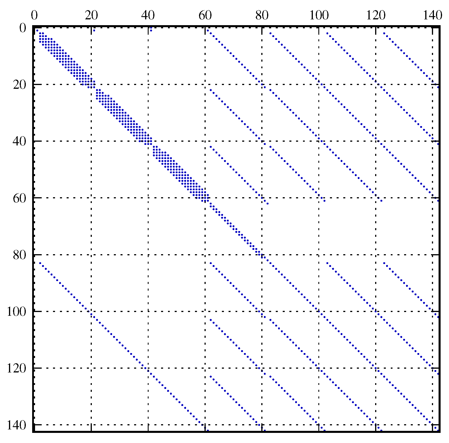
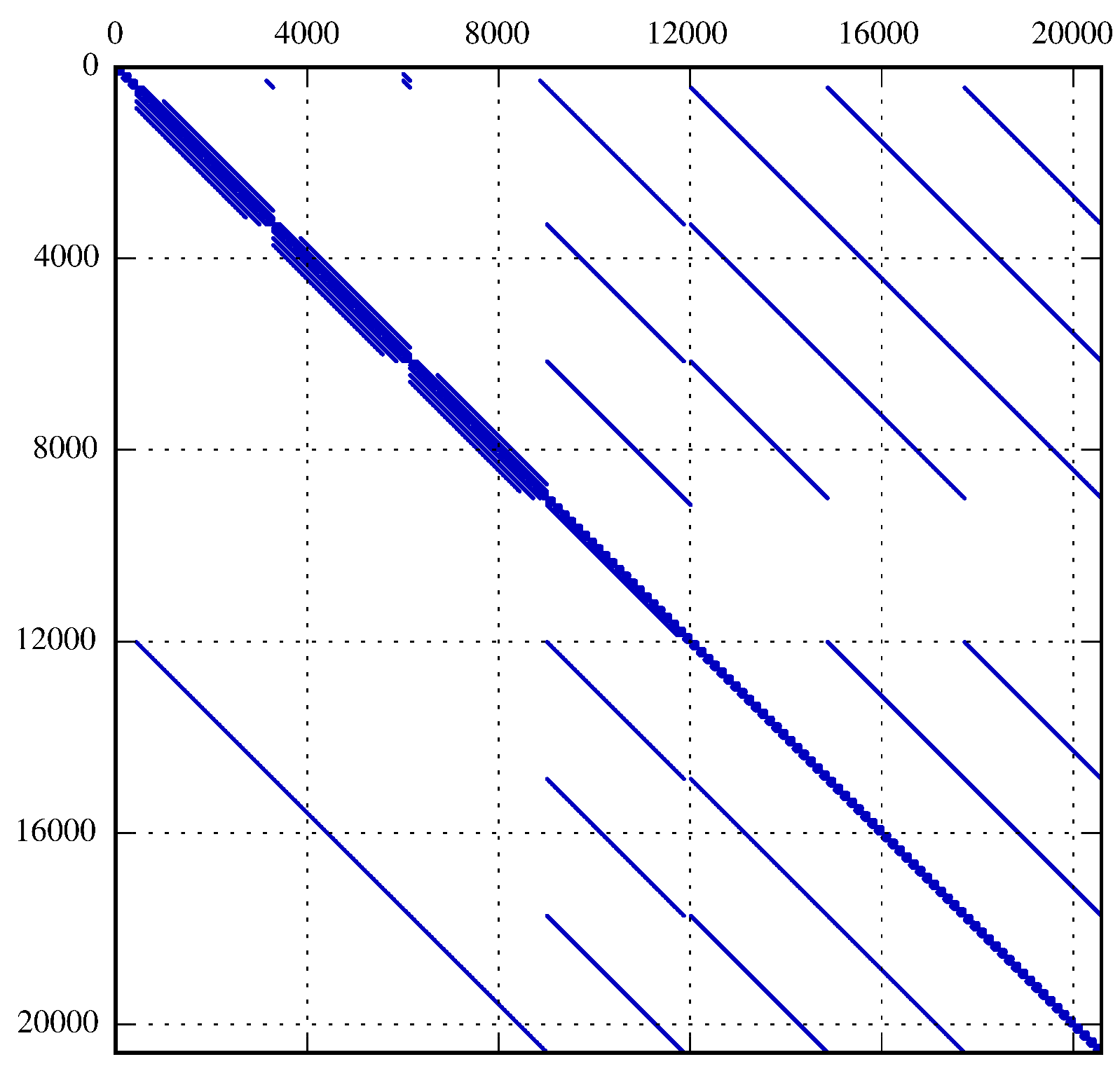
3.1. Spatial Discretization

The equations of the spatially distributed HPLC column model that describe the mobile and stationary phase state dynamics (Equations (1) and (2)), constitute a system of non-linear PDEs. In this study, the PDE system was approximated using the method-of-lines [33,34] and high-order finite volume WENO scheme [40,41,42] on a uniform mesh where $z_j=j\Delta z$ is the discretized spatial coordinate and $j\in [1..n_v]$. The main advantage of this scheme is its capability to achieve high-order formal accuracy in smooth regions while maintaining stable, nonoscillatory, and sharp discontinuity transitions. In contrast to other high-order spatial discretization schemes that make use of flux limiters [61], such as the MUSCL scheme [62] and the TVD scheme [63], the WENO scheme does not require tuning of parameters and more importantly the discretization scheme is twice continuously differentiable; a necessity when employing Newton-based methods for solving NLPs. Although a high-order WENO scheme may use several times more CPU time than the aforementioned schemes [64], which are usually second-order accurate in the smooth part of the solution, it is still computationally advantageous for the purpose of this study where the DOP is transcribed into an NLP using direct collocation in time. Hence, less grid points are required to spatially resolve complicated smooth structures with small numerical dissipation, and thereby reducing the size of the resulting NLP.

4. Problem Formulation

The cyclic operation of HPLC separation processes in batch elution mode imposes adequate retention time repeatability by conditioning the column to the initial modifier concentration prior to the subsequent injection [65,66]. In the scope of chromatographic separations, cyclic-steady-state (CSS) prediction has previously only been applied to continuous simulated moving bed (SMB) [11,18,67] and multicolumn counter-current solvent gradient purification (MCSGP) [68] processes. Hence, the CSS operation implies computation of a limit cycle dynamic solution, subject to initial conditions for the state variables, that conform to the periodic boundary condition over the processing cycle. It is however noteworthy that in order for the comprehensive CSS description to be experimentally feasible, a model representation of the most retained component in the loaded sample mixture is required. This is vital for prohibiting potential stationary phase accumulation of otherwise irreversibly adsorbing components, resulting in a gradual decrease in column adsorption capacity. For these reasons, the robustification methodology considered in this study was applied to two inherently different optimal control strategies:

i)

Optimal control strategy I is exclusively concerned with the batch elution operation mode, where the limit cycle criteria are relaxed and the upper fractionating interval endpoint bounds the temporal horizon, i.e., $t_f={\tau }_0+\Delta \tau$.

ii)

Optimal control strategy II is concerned with the comprehensive CSS operation mode, where the temporal horizon includes the column regeneration and re-equilibration modes.

Hence, optimal control strategy I that considerably reduces the DOP complexity, is preferable when the complete sample mixture composition is unknown and is extensively applied in open-loop optimal control studies on non-isocratic batch elution chromatography, see, for example, Damtew et al. [19], Osberghaus et al. [69] and the references cited therein.

4.1. Cyclic-Steady-State Criteria Formulation

The computation of CSS solutions over the temporal horizon $t\in [t_0,t_f]$ requires that Equations (1) and (2) are augmented with additional criteria governing that the state at the initial time is retained at the end of the cycle. Accordingly, the limit cycle criteria can be classified into terminal equality constraints:

$$\begin{array}{cccc}\hfill 0& {\displaystyle =\underset{t_0}{\overset{t_f}{\int }}{v}_{\mathrm{int}}{A}_c{c}_{\alpha }(t,z_f)\mathrm{d}t-{\delta }_{\mathrm{load},\alpha },}\hfill & & \hfill \left(6\mathrm{a}\right)\\ \hfill 0& =c_S(t_0,z)-c_S(t_f,z),\hfill & \forall z\in [z_0,z_f],\hfill & \hfill \left(6\mathrm{b}\right)\\ \hfill 0& =c_{\mathrm{mix},S}\left(t_0\right)-c_{\mathrm{mix},S}\left(t_f\right),\hfill & & \hfill \left(6\mathrm{c}\right)\\ \hfill 0& =u\left(t_0\right)-u\left(t_f\right),\hfill & & \hfill \left(6\mathrm{d}\right)\end{array}$$

and initial conditions satisfying:

$$\begin{array}{cccc}\hfill 0& =c_S(t_0,z)-u\left(t_0\right),\hfill & \forall z\in [z_0,z_f],\hfill & \hfill \left(6\mathrm{e}\right)\\ \hfill 0& =c_{\mathrm{mix},S}\left(t_0\right)-u\left(t_0\right),\hfill & & \hfill \left(6\mathrm{f}\right)\end{array}$$

where ${\delta }_{\mathrm{load},\alpha }=c_{\mathrm{load},\alpha }{v}_{\mathrm{int}}{A}_c\Delta t_{\mathrm{load}}$ is the total injected sample amount. Specifically, Equation (6a) states the flux of the most retained component $\alpha =C$ at the column outlet, $z=z_f$, equals the total loaded sample amount, ${\delta }_{\mathrm{load},\alpha }$, at $t=t_f$. This criterion, thereby, ensures that all components are completely eluted at the end of time horizon. The terminal equality constraints Equation (6b)–(6d) govern that the modifier concentration, $c_S$, at every column position $z\in [z_0,z_f]$ as well as the concentration in the mixing unit, $c_{\mathrm{mix},S}$, are consistent at the initial and terminal times. Moreover, Equation (6e) and (6f) are supplementary initial conditions, enforcing the initial modifier concentration at $t_0$. Equation (6a)–(6d) are introduced in the DOP whereas Equation (6e) and (6f) are introduced as initial values in the governing mobile phase transport equations.

4.2. Open-loop Optimal Control Problem Formulation

In chromatographic separations, there are several incommensurable objectives which require a trade-off to ensure satisfactory design, see e.g., Guiochon et al. [70] for a thorough review. Typical objective functions are the recovery yield, $Y_{\alpha }$, the production rate, $P_{\alpha }$, and the recovery concentration, $\langle c_{\alpha }\rangle$, with respect to the target component collected in the fractionating interval. In any case, the elution trajectories at the column outlet, $c_{\alpha }(t,z_f)$ for $\alpha \in \{A,B,C\}$, form the basis for evaluating the incommensurable objective functions. These are defined here as:

$$\begin{array}{cc}\hfill {\displaystyle {\delta }_{\mathrm{load},\alpha }\frac{\mathrm{d}{Y}_{\alpha }}{\mathrm{d}t}}& =c_{\alpha }(t,z_f)v_{\mathrm{int}}{A}_c\Pi (t,{\tau }_0,\Delta \tau ),\hfill \end{array}$$

(7)

$$\begin{array}{cc}\hfill \frac{\mathrm{d}{P}_{\alpha }}{\mathrm{d}t}& {\displaystyle =\frac{1}{V_c}\frac{1}{t_f}{\delta }_{\mathrm{load},\alpha }\frac{\mathrm{d}{Y}_{\alpha }}{\mathrm{d}t},}\hfill \end{array}$$

(8)

$$\begin{array}{cc}\hfill \frac{\mathrm{d}\langle c_{\alpha }\rangle }{\mathrm{d}t}& {\displaystyle =\frac{1}{v_{\mathrm{int}}{A}_c}\frac{1}{\Delta \tau }{\delta }_{\mathrm{load},\alpha }\frac{\mathrm{d}{Y}_{\alpha }}{\mathrm{d}t},}\hfill \end{array}$$

(9)

and subject to initial values $Y_{\alpha }\left(t_0\right)=0$, $P_{\alpha }\left(t_0\right)=0$, and $\langle c_{\alpha }\rangle \left(t_0\right)=0$. Moreover, $\Pi (t,{\tau }_0,\Delta \tau )$ is a smooth rectangular function in the fractionization horizon $[{\tau }_0,{\tau }_0+\Delta \tau ]$. It is noteworthy that both $P_{\alpha }$, defined as the amount of target component collected per cycle time scaled to the size of the column, and $\langle c_{\alpha }\rangle$, defined as the integral mean value of the target component concentration over the fractionating horizon, are intrinsically governed by $Y_{\alpha }$. A weighted sum scalarization method is frequently used to combine the objectives in Equations (7)–(9) into a single performance index. The procedures’ deterministic nature allows the use of direct NLP routines and ensures an accurate and efficient Pareto set generation [22].

For the purpose of this study, we solely consider the yield of the intermediately eluting component $\alpha =B$ as target in the optimal control problem. Hence, the aim is to derive an optimal elution trajectory, u, and fractionating interval endpoints, $[{\tau }_0,{\tau }_0+\Delta \tau ]$, that maximize $Y_{\alpha }\left(t_f\right)$ while fulfilling the constraint imposed on purity of the target component fractionization:

$$X_{\alpha }\left(t_f\right)={\delta }_{\mathrm{load},\alpha }{Y}_{\alpha }\left(t_f\right){\left(\sum _{\beta \in \{A,B,C\}}^{}{\delta }_{\mathrm{load},\beta }{Y}_{\beta }\left(t_f\right)\right)}^{-1},$$

(10)

where the numerator of the right hand side represents the captured amount of the target component in $[{\tau }_0,{\tau }_0+\Delta \tau ]$ and the denominator represents the total amount captured. Hence, $X_{\alpha }\left(t_f\right)$ is incorporated in the DOP as a terminal inequality constraint, $X_{\alpha ,L}-X_{\alpha }\left(t_f\right)\le 0$, with an assigned lower purity requirement $X_{\alpha ,L}$. Given the optimization specifications in Equations (7) and (10) the open-loop optimal control problem, with differential algebraic constraints [31,71], over the temporal domain $[t_0,t_f]$ may now be formulated as:

$$\begin{array}{cccc}\text{min.}\hfill & {\displaystyle -\underset{t_0}{\overset{t_f}{\int }}\frac{\mathrm{d}{Y}_B}{\mathrm{d}t}+\mathrm{R}\sum _{i=1}^{N_u-1}\Delta u_i^2,}\hfill & & \hfill \left(11\mathrm{a}\right)\\ \text{w.r.t.}\hfill & x:[t_0,t_f]\to {\mathbb{R}}^{n_x},\hfill & X_B:[t_0,t_f]\to \mathbb{R},\phantom{1}\hfill & \\ & ({\tau }_0,\Delta \tau )\in {\mathbb{R}}^2,\hfill & u_m\in \mathbb{R},\hfill & \\ \text{s.t.}\hfill & \mathit{F}(t,\dot{x}\left(t\right),x\left(t\right),X_B\left(t\right),u\left(t\right),{\tau }_0,\Delta \tau )=\mathbf{0},\hfill & x\left(t_0\right)=x_0,\hfill & \hfill \left(11\mathrm{b}\right)\\ & X_{B,L}-X_B\left(t_f\right)\le 0,\hfill & & \hfill \left(11\mathrm{c}\right)\\ & g_e(x\left(t_0\right),x\left(t_f\right),u_1,u_{N_u})=\mathbf{0},\hfill & & \hfill \left(11\mathrm{d}\right)\\ & u_L\le u_m\le u_U,\hfill & |\Delta u_n|\le \Delta u_U,\hfill & \hfill \left(\mathrm{11}e\right)\\ & {\tau }_{0,L}\le {\tau }_0\le {\tau }_{0,U},\hfill & \Delta {\tau }_L\le \Delta \tau \le \Delta {\tau }_U,\hfill & \hfill \left(11\mathrm{f}\right)\\ & \forall t\in [t_0,t_f],\hfill & \forall m\in [1..N_u],\forall n\in [1..N_u-1].\hfill & \end{array}$$

In addition to the free operating parameters, i.e., the discrete control signal u and the free time-invariant parameters $({\tau }_0,\Delta \tau )$, the optimization variables include the state variables $x\left(t\right)=(c_{\alpha }(t,z_j),c_S(t,z_j),c_{\mathrm{mix},S}\left(t\right),q_{\alpha }(t,z_j),Y_{\alpha }\left(t\right))$ for $\alpha \in \{A,B,C\}$ and the algebraic variable $X_B$. F denotes the implicit DAE system resulting from the spatially discretized PDAE system. Moreover, $g_e$ denotes the terminal equality constraints and assembles the limit cycle criteria defined in Equation (6). Time-invariant bounds on the fractionation variables are introduced in Equation (11f) and absolute and rate limitations of the control are enforced in Equation (11e). As outlined in Section 2.1, Equation (11a) is augmented with a quadratic penalty on the differences of the piecewise constant controls, $\Delta u$, discretized with $N_u$ segments in the temporal domain $[t_0,t_f]$. This will influence the smoothness of u, and the weight R is used as an optimization variable in the robust counterpart problem in order to find optimal robustified elution trajectories.

4.3. Robust Counterpart Problem Formulation

The solution of Equation (11) will yield optimal open-loop trajectories that lie on the boundary of the feasible region. This means that even the smallest of unmodeled disturbances can cause infeasbility, leading to failed batches. To account for this, we discuss how a robust counterpart of Equation (11) can be formulated and then approximated based on linearization to reduce computational complexity. The resulting formulation is still not computationally tractable, but we present how it nevertheless can be used to find robust solutions using bilevel optimization.

In parts of this section we will assume that the system dynamics in Equation (11b) are described by an explicit ordinary differential equation (ODE) system

$$\begin{array}{cc}\hfill \dot{x}\left(t\right)& =f(t,x\left(t\right),u\left(t\right),{\tau }_0,\Delta \tau ),\hfill \end{array}$$

(12a)

$$\begin{array}{cc}\hfill X_B\left(t\right)& =h\left(x\right(t\left)\right),\hfill \end{array}$$

(12b)

rather than a DAE. Since the considered DAE is of index one, the transformation to an ODE is straightforward and is handled by the framework discussed in Section 5.1.2. The uncertainties discussed in Section 2.1 are modeled as a disturbance w that is added to the control variable u, whose $L_2$ norm is bounded by . The constraint that we want to make robust with respect to these uncertainties is the purity constraint $X_B\left(t_f\right)\ge X_{B,L}$. The considered robust counterpart of Equation (11) is thus essentially to modify $X_B\left(t_f\right)$ in the purity constraint to instead be the minimum of $X_B\left(t_f\right)$ over all disturbances w with $L_2$ norm less than (A rigorous formulation of the considered robust counterpart involves transforming the problem to Mayer form and eliminating the state variables by utilizing the existence of a unique solution of the ODE. The result is verbose and neither enlightening nor useful for computations, and is thus omitted). The result is a problem that is not computationally tractable due to the nonlinear dynamics, even if the state dimension would have been small. To reduce the computational complexity, we utilize the linearization approach presented in [49]. We first solve the original problem Equation (11) to obtain nominal trajectories $x^{*}$ and $u^{*}$. We then introduce the deviation $\delta x$ caused by the disturbance w, leading to the perturbed trajectory $x=x^{*}+\delta x$. The deviation $\delta x$ can be approximately determined by linearizing the dynamics around the nominal trajectories $x^{*}$ and $u^{*}$. This leads to the uncertain linear time-varying system

$$\delta \dot{x}\left(t\right)=\mathbf{A}\left(t\right)\delta x\left(t\right)+\mathbf{B}\left(t\right)w\left(t\right),\delta x\left(0\right)=\mathbf{0},$$

(13)

for determining the deviation corresponding to w, where

$$\begin{array}{cc}\hfill \mathbf{A}\left(t\right)& =\frac{\partial }{\partial x}f\left(t,x^{*}\left(t\right),u^{*}\left(t\right),{\tau }_0^{*},\Delta {\tau }^{*}\right),\hfill \end{array}$$

(14a)

$$\begin{array}{cc}\hfill \mathbf{B}\left(t\right)& =\frac{\partial }{\partial u}f\left(t,x^{*}\left(t\right),u^{*}\left(t\right),{\tau }_0^{*},\Delta {\tau }^{*}\right).\hfill \end{array}$$

(14b)

The utilization of the above linearization, which is valid for small disturbances, and [Theorem 3.1] [72] yields that the robust counterpart can be equivalently formulated by the introduction of the back-off term $\Gamma \sqrt{\mathbf{C}\left(t\right)\mathbf{P}\left(t\right){\mathbf{C}}^T\left(t\right)}$, where

$$\mathbf{C}\left(t\right)=\frac{\partial }{\partial x}h\left(x^{*}\left(t\right)\right),$$

(15)

and $\mathbf{P}:[t_0,t_f]\to {\mathbb{S}}_{+}^{n_x}$ satisfies the Lyapunov differential equation

$$\dot{\mathbf{P}}\left(t\right)=\mathbf{A}\left(t\right)\mathbf{P}\left(t\right)+\mathbf{P}\left(t\right){\mathbf{A}}^T\left(t\right)+\mathbf{B}\left(t\right){\mathbf{B}}^T\left(t\right),\mathbf{P}\left(t_0\right)=\mathbf{B}\left(t_0\right){\mathbf{B}}^T\left(t_0\right).$$

(16)

The back-off term is used to augment the purity constraint Equation (11c) to get

$$X_{B,L}+\Gamma \sqrt{\mathbf{C}\left(t_f\right)\mathbf{P}\left(t_f\right){\mathbf{C}}^T\left(t_f\right)}\le h\left(x\left(t_f\right)\right).$$

(17)

This back-off term can be regarded as an additional safety margin required for guaranteeing the meeting of the constraint. However, to compute it, we need to introduce P, givings us $n_x(n_x+1)/2$ extra states. The result is the following approximate robust counterpart of Equation (11).

$$\begin{array}{cccc}\text{min.}\hfill & {\displaystyle -\underset{t_0}{\overset{t_f}{\int }}\frac{\mathrm{d}{Y}_B}{\mathrm{d}t}+\mathrm{R}\sum _{i=1}^{N_u-1}\Delta u_i^2,}\hfill & & \hfill \left(18\mathrm{a}\right)\\ \text{w.r.t.}\hfill & x:[t_0,t_f]\to {\mathbb{R}}^{n_x},X_B:[t_0,t_f]\to \mathbb{R},\hfill & \mathbf{P}:[t_0,t_f]\to {\mathbb{S}}_{+}^{n_x},\hfill & \\ & ({\tau }_0,\Delta \tau )\in {\mathbb{R}}^2,\hfill & u_m\in \mathbb{R},\mathrm{R}\in \mathbb{R},\hfill & \\ \text{s.t.}\hfill & \dot{x}\left(t\right)=f(t,x\left(t\right),u\left(t\right),{\tau }_0,\Delta \tau ),\hfill & x\left(t_0\right)=x_0,\hfill & \hfill \left(18\mathrm{b}\right)\\ & \dot{\mathbf{P}}\left(t\right)=\mathbf{A}\left(t\right)\mathbf{P}\left(t\right)+\mathbf{P}\left(t\right){\mathbf{A}}^T\left(t\right)+\mathbf{B}\left(t\right){\mathbf{B}}^T\left(t\right),\hfill & \mathbf{P}\left(t_0\right)=\mathbf{B}\left(t_0\right){\mathbf{B}}^T\left(t_0\right),\hfill & \hfill \left(18\mathrm{c}\right)\\ & X_{B,L}+\sqrt{\mathbf{C}\left(t_f\right)\mathbf{P}\left(t_f\right){\mathbf{C}}^T\left(t_f\right)}\le h\left(x\left(t_f\right)\right),\hfill & & \hfill \left(18\mathrm{d}\right)\\ & g_e(x\left(t_0\right),x\left(t_f\right),u_1,u_{N_u})=\mathbf{0},\hfill & {\mathrm{R}}_L\le \mathrm{R}\le {\mathrm{R}}_U,\hfill & \hfill \left(18\mathrm{e}\right)\\ & u_L\le u_m\le u_U,\hfill & |\Delta u_n|\le \Delta u_U,\hfill & \hfill \left(18\mathrm{f}\right)\\ & {\tau }_{0,L}\le {\tau }_0\le {\tau }_{0,U},\hfill & \Delta {\tau }_L\le \Delta \tau \le \Delta {\tau }_U,\hfill & \hfill \left(18\mathrm{g}\right)\\ & \forall t\in [t_0,t_f],\hfill & \forall m\in [1..N_u],\forall n\in [1..N_u-1].\hfill & \end{array}$$

The discussed robustification also has a stochastic interpretation [72]. Rather than considering disturbances with bounded norm Γ, we can instead consider stochastic disturbances. If w is a Gaussian white noise process with an identity covariance matrix, then P is a linear approximation of the covariance matrix of the state x. Consequently, the covariance matrix associated with the output function h is approximated by $\mathbf{C}\left(t\right)\mathbf{P}\left(t\right){\mathbf{C}}^T\left(t\right)$. While the discussed approximate robust approach is computationally tractable for medium-scale ODE-constrained DOPs, it is not for our original PDE-constrained DOP. For these reasons, the robust counterpart problem is cast in the frame of bilevel optimal control where the upper level concerns forward simulation of the Lyapunov differential equation, and the nominal NLP augmented with the robustified inequality constraint margin is considered in the lower level:

$$\begin{array}{ccccc}\text{min.}\hfill & \multicolumn{2}{c}{{\displaystyle -\underset{t_0}{\overset{t_f}{\int }}\frac{\mathrm{d}{Y}_B}{\mathrm{d}t}\mathrm{d}t,}}& & \hfill \left(19\mathrm{a}\right)\\ \text{w.r.t.}\hfill & \multicolumn{2}{c}{x:[t_0,t_f]\to {\mathbb{R}}^{n_x},}& \multicolumn{2}{c}{\mathbf{P}:[t_0,t_f]\to {\mathbb{S}}_{+}^{n_x},}& \\ & \multicolumn{2}{c}{({\tau }_0,\Delta \tau )\in {\mathbb{R}}^2,}& \multicolumn{2}{c}{u_m\in \mathbb{R},\mathrm{R}\in \mathbb{R},}& \\ \text{s.t.}\hfill & \multicolumn{2}{c}{\dot{x}\left(t\right)=f(t,x\left(t\right),u\left(t\right),{\tau }_0,\Delta \tau ),}& \multicolumn{2}{c}{x\left(t_0\right)=x_0,}& \hfill \left(19\mathrm{b}\right)\\ & \multicolumn{2}{c}{\dot{\mathbf{P}}\left(t\right)=\mathbf{A}\left(t\right)\mathbf{P}\left(t\right)+\mathbf{P}\left(t\right){\mathbf{A}}^T\left(t\right)+\mathbf{B}\left(t\right){\mathbf{B}}^T\left(t\right),}& \multicolumn{2}{c}{\mathbf{P}\left(t_0\right)=\mathbf{B}\left(t_0\right){\mathbf{B}}^T\left(t_0\right)}& \hfill \left(19\mathrm{c}\right)\\ & \multicolumn{2}{c}{{\mathrm{R}}_L\le \mathrm{R}\le {\mathrm{R}}_U,}& & \hfill \left(19\mathrm{d}\right)\\ & \multicolumn{3}{c}{\left(x,u,{\tau }_0,\Delta \tau \right)=\text{arg min.}{\displaystyle -\underset{t_0}{\overset{t_f}{\int }}\frac{\mathrm{d}{Y}_B}{\mathrm{d}t}\mathrm{d}t+\mathrm{R}\sum _{i=1}^{N_u-1}\Delta u_i^2,}}& & \hfill \left(19\mathrm{e}\right)\\ & \text{w.r.t.}\hspace{1em}x:[t_0,t_f]\to {\mathbb{R}}^{n_x},\hfill & X_B:[t_0,t_f]\to \mathbb{R},\hfill & \\ & \hspace{1em}\hspace{1em}\hspace{1em}({\tau }_0,\Delta \tau )\in {\mathbb{R}}^2,\hfill & u_m\in \mathbb{R},\hfill & \\ & \text{s.t.}\hspace{1em}\hspace{1em}\mathit{F}(t,\dot{x}\left(t\right),x\left(t\right),X_B\left(t\right),u\left(t\right),{\tau }_0,\Delta \tau )=\mathbf{0},\hfill & x\left(t_0\right)=x_0,\hfill & \hfill \left(19\mathrm{f}\right)\\ & \hspace{1em}\hspace{1em}\hspace{1em}{X}_{B,L}+\Gamma \sqrt{\mathbf{C}\left(t_f\right)\mathbf{P}\left(t_f\right){\mathbf{C}}^T\left(t_f\right)}\le h\left(x\left(t_f\right)\right),\hfill & & \hfill \left(19\mathrm{g}\right)\\ & \hspace{1em}\hspace{1em}\hspace{1em}{g}_e(x\left(t_0\right),x\left(t_f\right),u_1,u_{N_u})=\mathbf{0},\hfill & & \hfill \left(19\mathrm{h}\right)\\ & \hspace{1em}\hspace{1em}\hspace{1em}{\tau }_{0,L}\le {\tau }_0\le {\tau }_{0,U},\hfill & \Delta {\tau }_L\le \Delta \tau \le \Delta {\tau }_U,\hfill & \hfill \left(19\mathrm{i}\right)\\ & \multicolumn{2}{c}{\hspace{1em}\hspace{1em}\hspace{1em}{u}_L\le u_m\le u_U,}& |\Delta u_n|\le \Delta u_U,\hfill & \hfill \left(19\mathrm{j}\right)\\ & \hspace{1em}\hspace{1em}\hspace{1em}\forall t\in [t_0,t_f],\hfill & \forall m\in [1..N_u],\forall n\in [1..N_u-1].\hfill & \end{array}$$

It is noteworthy that while the nominal optimal control problem Equation (11) is feasible, the robust counterpart formulation Equation (19) might not be feasible for large disturbances as the constraints are required to be satisfied. The upper-level static optimization problem (Equations (19a)–(19d)) with respect to R is solved using a Nelder–Mead Simplex algorithm, whereas the lower-level DOP (Equations (19e)–(19j) constrained by the DAE system dynamics is transcribed into an NLP using direct collocation, as described in Section 5.2. This strategy avoids the full simultaneous discretization of the Lyapunov states, which are too numerous to be treated with direct collocation. Finally, it is important to clarify that the Lyapunov state simulation and the subsequent NLP execution is repeated in the lower level until an optimal solution is obtained for a fixed R, i.e., Equation (19g) is satisfied to a small specified tolerance.

5. Methods and Tools

This section outlines the languages and tools used to generate the simulation and optimization results. We first present the general software framework and then discuss the methods in the framework that allow for the efficient solution of Equation (19).

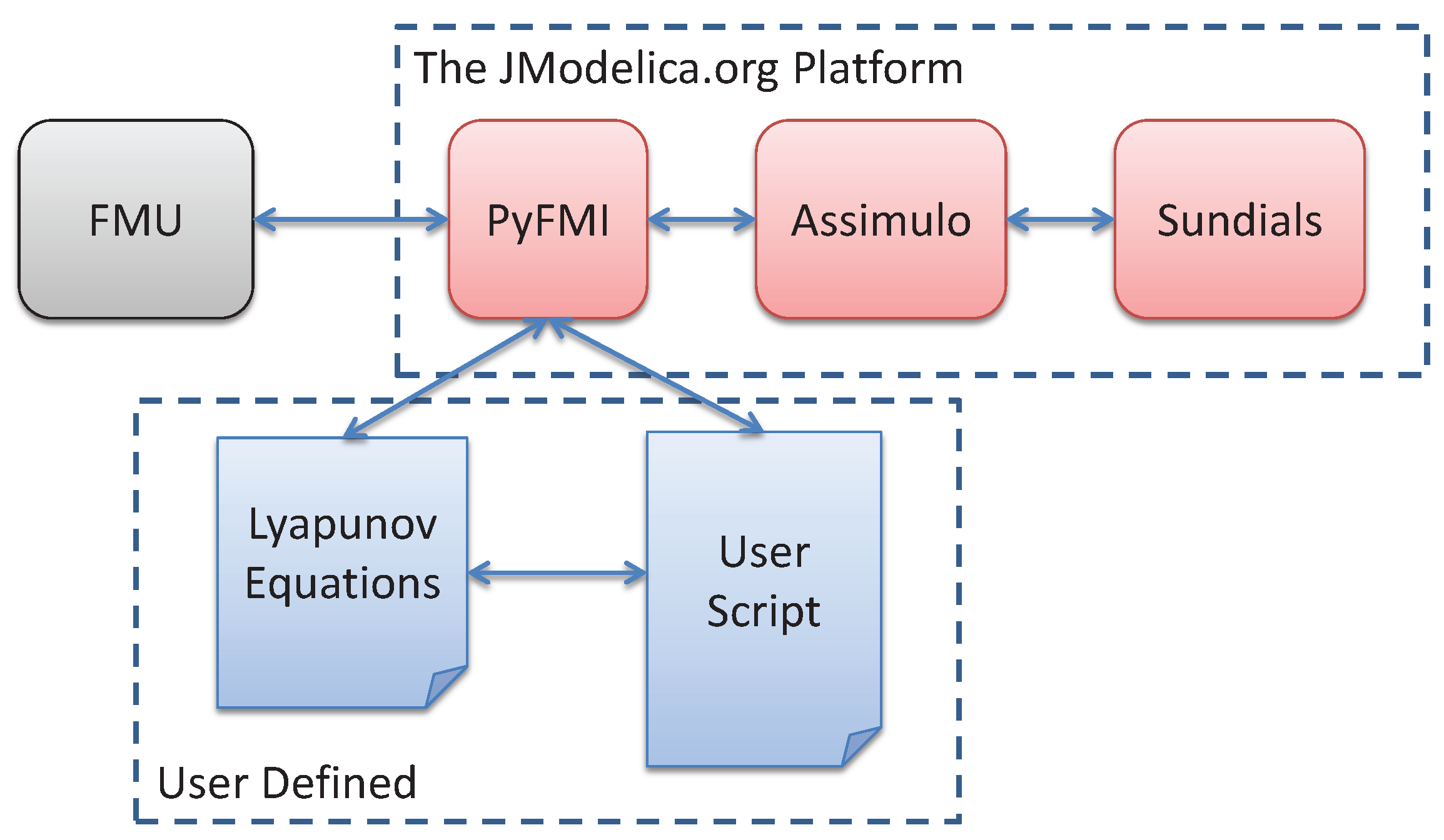
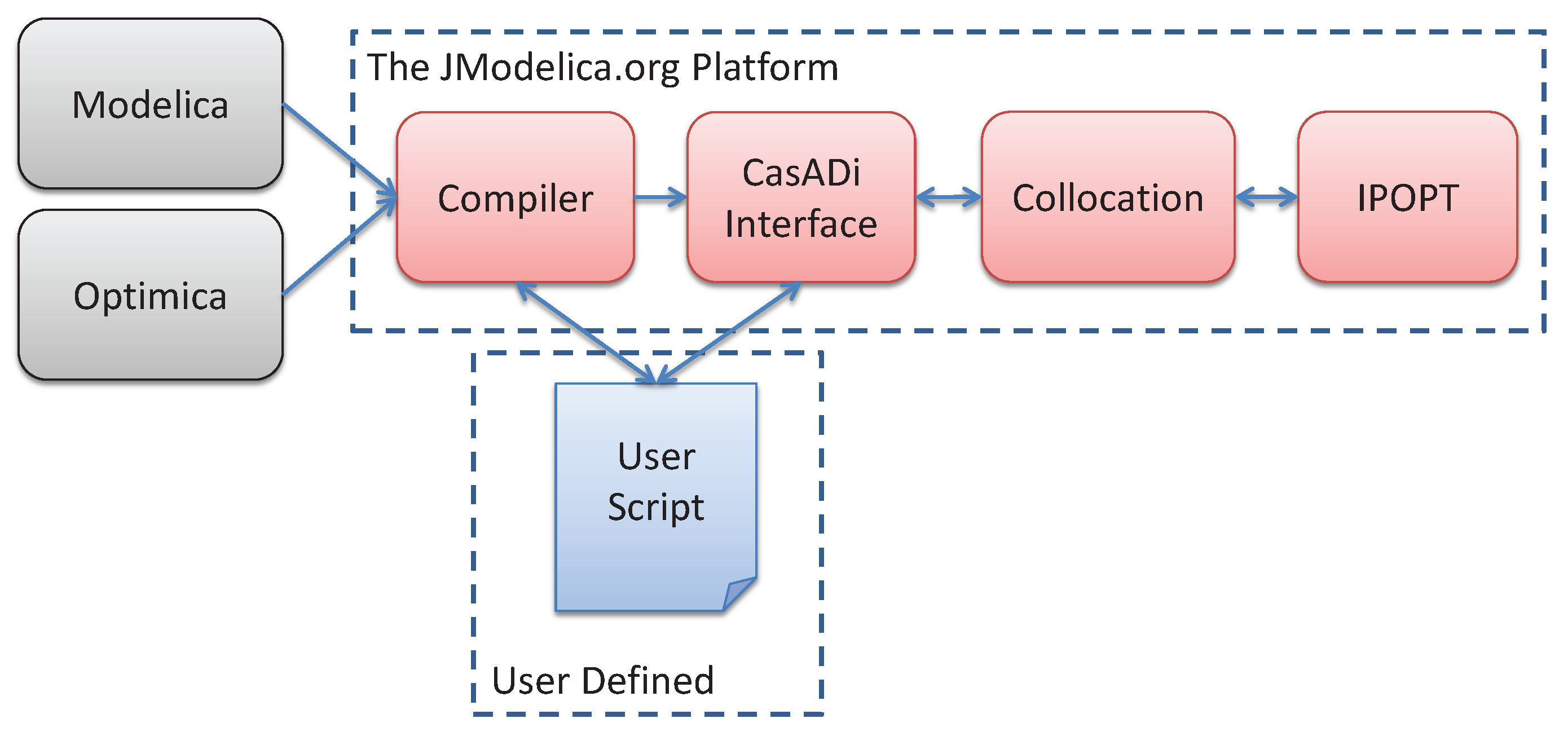
5.1. The JModelica.org Toolchain

JModelica.org [73] is an open-source platform for simulation and optimization of models described in either the Modelica [74] or Optimica language [75] or as Functional Mock-up Units (FMUs) following the Functional Mock-up Interface (FMI) [76]. The platform consists of a Modelica and Optimica compiler meaning that the input is a model described in either of the two languages and the output of the compiler is either an FMU or a symbolic representation of an optimization problem. Modelica is an equation based, high-level language for describing complex physical systems. Optimica is an extension which additionally allows for specifying dynamic optimization problem with a cost function and constraints.

5.1.1. Optimization

The dynamic optimization framework in JModelica.org is centered around CasADi [77] and an overview is shown in Figure 2. CasADi (Computer algebra system with Automatic Differentaion) is an open-source, low-level tool for efficiently computing derivatives using AD and is tailored for dynamic optimization. The user encodes the dynamic optimization problem using Modelica and Optimica. The JModelica.org compiler then transfers a symbolic representation of the problem to CasADi Interface [78], after performing symbolic transformations such as index reduction. CasADi Interface serves as a three-way, symbolic Python interface between the optimization problem, user, and numerical algorithm. The main numerical algorithm for dynamic optimization in JModelica.org is based on direct, local collocation and is described in Section 5.2. The algorithm is implemented using CasADi to transcribe the DOP into an NLP. First- and second-order derivatives of the NLP functions can then be conveniently and efficiently computed using CasADi’s algorithmic differentiation while preserving sparsity. The NLP is then finally solved by the open-source, interior-point method IPOPT [43].

Figure 2. The dynamic optimization framework of the JModelica.org platform. The problem is formulated using Modelica and Optimica, which is then transferred to CasADi Interface by the JModelica.org compiler. CasADi Interface is a symbolic interface between the compiler, user, and collocation algorithm. After collocation, the problem is finally solved by IPOPT.

Figure 2. The dynamic optimization framework of the JModelica.org platform. The problem is formulated using Modelica and Optimica, which is then transferred to CasADi Interface by the JModelica.org compiler. CasADi Interface is a symbolic interface between the compiler, user, and collocation algorithm. After collocation, the problem is finally solved by IPOPT.

5.1.2. Simulation

The simulation capabilities in the JModelica.org platform is based on FMUs and collected in the standalone Python package PyFMI. It is a package for interacting with models following the FMI and designed to provide a high-level, easy to use environment for working with FMUs. A key feature is the connection to Assimulo [79] which provides capabilities for performing simulations using state-of-the art solvers such as CVode from the Sundials suite [80]. PyFMI together with Assimulo provides an efficient and flexible environment for simulation of FMUs. An overview of the simulation capabilities is shown in Figure 3. The FMUs are typically created from a Modelica model using the JModelica.org compiler. However, as FMI is an open standard, any tool that support generation of FMUs can be used.

Figure 3. The simulation capabilities of the JModelica.org platform. An FMU is loaded using the package PyFMI, which in turn connects to the simulation package Assimulo which provides access to the solvers. The work-flow is controlled through a user-defined script which additionally allows for providing extra equations to the problem, in this paper the Lyapunov equations.

Figure 3. The simulation capabilities of the JModelica.org platform. An FMU is loaded using the package PyFMI, which in turn connects to the simulation package Assimulo which provides access to the solvers. The work-flow is controlled through a user-defined script which additionally allows for providing extra equations to the problem, in this paper the Lyapunov equations.

5.2. Transcription of the Dynamic Optimization Problem

The optimization problem Equation (11) falls within the class of dynamic optimization problems of the general form:

$$\begin{array}{ccccc}\text{min.}\hfill & \multicolumn{2}{c}{\underset{t_0}{\overset{t_f}{\int }}L(t,\dot{x}\left(t\right),x\left(t\right),y\left(t\right),u\left(t\right),p)\mathrm{d}t+\sum _{j=1}^{N_u-1}{(\Delta u_j)}^T\mathbf{R}(\Delta u_j),}& & \hfill \left(20\mathrm{a}\right)\\ \text{w.r.t.}\hfill & x:[t_0,t_f]\to {\mathbb{R}}^{n_x},\hfill & y:[t_0,t_f]\to {\mathbb{R}}^{n_y},\hfill & \\ & p\in {\mathbb{R}}^{n_p},\hfill & u_i\in {\mathbb{R}}^{n_u},\hfill & \\ \text{s.t.}\hfill & \mathit{F}(t,\dot{x}\left(t\right),x\left(t\right),y\left(t\right),u\left(t\right),p)=\mathbf{0},\hfill & x\left(t_0\right)=x_0,\hfill & \hfill \left(20\mathrm{b}\right)\\ & (x_L,y_L)\le (x\left(t\right),y\left(t\right))\le (x_U,y_U),\hfill & p_L\le p\le p_U,\hfill & \hfill \left(20\mathrm{c}\right)\\ & u_L\le u_i\le u_U,\hfill & \Delta u_L\le \Delta u_j\le \Delta u_U,\hfill & \hfill \left(20\mathrm{d}\right)\\ & g_e(x\left(t_0\right),x\left(t_f\right),y\left(t_f\right),u_1,u_{N_u})=\mathbf{0},\hfill & g_i(x\left(t_0\right),x\left(t_f\right),y\left(t_f\right),u_1,u_{N_u})\le \mathbf{0},\hfill & \hfill \left(20\mathrm{e}\right)\\ & \multicolumn{2}{c}{\forall t\in [t_0,t_f],\forall i\in [1..N_u],\forall j\in [1..N_u-1],}& & \end{array}$$

where y is the algebraic variable and p is the free time-invariant parameters. The objective Equation (20a) is a typical optimal control Lagrange term together with a quadratic penalty on $\Delta u_i$, where $\mathbf{R}\in {\mathbb{R}}^{n_u\times n_u}$ acts as a weight and is typically diagonal. The optimization variables are the free operating parameters—The discrete control signal $u_i$ and free time-invariant parameters p—And the trajectories x and y. The trajectories are determined by the free operating parameters via the implicit DAE system in Equation (20b).

In this section we present an overview of the method employed by JModelica.org to solve Equation (20) and in particular the low-level problem in Equation (19). A more detailed description is available in [81]. The method is based on direct local collocation [31,32]. The fundamental idea is to discretize the differential equations, thus transforming, or transcribing, the dynamic optimization problem into a finite-dimensional NLP, which then is solved by IPOPT. The discretization scheme is based on collocation methods, which correspond to special cases of implicit Runge-Kutta methods and are also commonly used for numerical solution of DAE and stiff ODE systems [82].

We start by dividing the optimization time horizon into $n_e$ elements. Within each element $i\in [1..n_e]$ the trajectories x and y are approximated using low-order polynomials, which are called the collocation polynomials for that element. The collocation polynomials are formed by first choosing $n_c$ collocation points, which are chosen to be the same for all elements. Let $t_{i,k}$ be collocation point $k\in [1..n_c]$ in element i and $(x_{i,k},y_{i,k},u_{i,k})$ denote the value of $(x\left(t_{i,k}\right),y\left(t_{i,k}\right),u\left(t_{i,k}\right))$. The collocation polynomials in element i are then constructed by interpolating the values $(x_{i,k},y_{i,k})$. The polynomials for $\dot{x}$ are obtained by differentiating the polynomials for x. The control variable values $u_{i,k}$ are obtained by constructing a map $\sigma :[1..n_e]\times [1..n_c]\to [1..N_u]$ such that $u_{\sigma (i,k)}=u\left(t_{i,k}\right)$. There are different schemes for choosing the collocation points ${\tau }_k$, with different numerical properties, in particular regarding stability and order of convergence. We use Radau collocation, which always places a collocation point at the end of each element, and the rest are chosen in a manner that maximizes convergence order.

As decision variables in the transcribed NLP we choose the system variable values in all the collocation points, ${\dot{x}}_{i,k},x_{i,k},y_{i,k}$, the discrete control signal, $u_i$, the state at the start of each element, $x_{i,0}$, and the free parameters p. The transcription of Equation (20) results in the NLP

$$\begin{array}{ccccc}\text{min.}\hfill & \multicolumn{2}{c}{{\displaystyle \sum _{i=1}^{n_e}{h}_i\sum _{k=1}^{n_c}{\omega }_{k}L\left(t_{i,k},{\dot{x}}_{i,k},x_{i,k},y_{i,k},u_{\sigma (i,k)},p\right)+\sum _{j=1}^{N_u-1}{(\Delta u_j)}^T\mathbf{R}(\Delta u_j),}}& & \hfill \left(21\mathrm{a}\right)\\ \text{w.r.t.}\hfill & {\displaystyle {\dot{x}}_{i,k}\in {\mathbb{R}}^{n_x},x_{i,k}\in {\mathbb{R}}^{n_x},y_{i,k}\in {\mathbb{R}}^{n_y},}\hfill & & \\ & {\displaystyle x_{i,0}\in {\mathbb{R}}^{n_x},u_i\in {\mathbb{R}}^{n_u},p\in {\mathbb{R}}^{n_p},}\hfill & & \\ \text{s.t.}\hfill & \mathit{F}(t_{i,k},{\dot{x}}_{i,k},x_{i,k},y_{i,k},u_{\sigma (i,k)},p)=\mathbf{0},\hfill & x_{1,0}=x_0,\hfill & \hfill \left(21\mathrm{b}\right)\\ & (x_L,y_L)\le (x_{i,k},y_{i,k})\le (x_U,y_U),\hfill & p_L\le p\le p_U,\hfill & \hfill \left(21\mathrm{c}\right)\\ & u_L\le u_i\le u_U,\hfill & \Delta u_L\le \Delta u_j\le \Delta u_U,\hfill & \hfill \left(21\mathrm{d}\right)\\ & g_e(x_{1,0},x_{n_e,n_c},y_{n_e,n_c},u_1,u_{N_u})=\mathbf{0},\hfill & g_i(x_{1,0},x_{n_e,n_c},y_{n_e,n_c},u_1,u_{N_u})\le \mathbf{0},\hfill & \hfill \left(21\mathrm{e}\right)\\ & x_{n-1,n_c}=x_{n,0},\forall n\in [2..n_e],\hfill & & \hfill \left(21\mathrm{f}\right)\\ & {\displaystyle {\dot{x}}_{i,k}=\frac{1}{h_i}\sum _{l=0}^{n_c}{\alpha }_{l,k}{x}_{i,l},}\hfill & & \hfill \left(21\mathrm{g}\right)\\ & \multicolumn{2}{c}{{\displaystyle \forall i\in [1..n_e],\forall k\in [1..n_c],\forall j\in [1..N_u-1].}}& \end{array}$$

The transcription of the Lagrange term in Equation (20a) utilizes Gauss-Radau quadrature within each element to approximate the integral by a sum using the quadrature weights ${\omega }_k$ and element lengths $h_i$. Equation (20b) and (20c) are transcribed into Equation (21b) and (21c), respectively, by enforcing them only in each of the collocation points, rather than during the entire time horizon. The constraints Equation (20d) and (20e) are finite in number and are thus straightforward to transcribe into Equation (21d) and (21e), respectively, using the collocation point values.

Since the states need to be continuous (but not differentiable) with respect to time, the new continuity constraint Equation (21f) needs to be introduced. Because we use Radau collocation, where no collocation point exists at the start of each element, this also requires the introduction of the new variables $x_{i,0}$, which represent the value of the state at the start of element i. Finally, we introduce Equation (21g) to capture the dependency between x and $\dot{x}$, which is implicit in Equation (20). The weights ${\alpha }_{l,k}$ are obtained from differentiating the collocation polyonimals for the state and related to the butcher tableau of the Runge-Kutta method that corresponds to the collocation method.

5.3. Simulation Setup and Coupling of the Lyapunov Equation

In this study, the process model is implemented in Modelica and compiled into an FMU, for simulation, using the tool Dymola [83]. Any tool that is able to transform the Modelica model into an FMU can be used, provided that support for directional derivatives is included. Hence, the process model is transformed and exposed as a system of ordinary differential equations,

$$\begin{array}{cc}\hfill \dot{x}\left(t\right)& =f(t,x\left(t\right),u\left(t\right),{\tau }_0,\Delta \tau ),\hfill \end{array}$$

(22)

$$\begin{array}{cc}\hfill X_B\left(t\right)& =h\left(x\right(t\left)\right).\hfill \end{array}$$

(23)

This transformation step is performed by the exporting tool. As the process model is stiff an implicit solver is needed to simulate the problem which in turn requires the Jacobian matrix of Equation (22).

The Jacobian can either be approximated using finite differences, symbolic differentiation or using algorithmic differentiation. However, in order to simulate this model efficiently and accurately, access to the Jacobian, either symbolically or via algorithmic differentiation is crucial. In the FMU, directional derivatives are available and using these, the partial derivatives can be constructed (i.e., the Jacobian). The directional derivatives are defined as,

$$\begin{array}{c}\hfill g_z=\frac{\partial g\left(z\right)}{\partial z}v,\end{array}$$

(24)

where $g\left(z\right)$ is a set of equations, in our case, either Equations (22) or (23), z is either the states x or the inputs u and v is the seed vector. From the directional derivatives, the partial derivatives can directly be computed by a sequence of calls with v replaced by unit vectors. However, as discussed below, there are more efficient approaches.

For efficiency, FMI provides structural information in the sense that the dependency information between the functions $f_i$ and $x_j$, $u_k$ are available. Utilizing this information, multiple columns can be constructed for each call to the directional derivative method due to that all equations are not dependent on all of the states. Finding the minimal set of calls to the directional derivative method for a general problem is difficult. However, using the algorithm by Curtis-Powell-Reid [84] one can find a set that substantially reduces the amount of calls in a straight-forward manner. In the considered case, the number of calls was reduced by $90\%$ by applying the algorithm. Additionally, the structural information directly corresponds to the sparsity pattern which is shown in Figure 4. The pattern indicates that the model is sparse and using a sparse solver for the problem is thus beneficial. Using both the structural information and the directional derivatives, the process model, as an FMU, can efficiently and accurately be simulated.

Figure 4. The sparsity pattern of the Jacobian of the spatially discretized, with $n_v=20$, and ODE transformed system.

Figure 4. The sparsity pattern of the Jacobian of the spatially discretized, with $n_v=20$, and ODE transformed system.

However, our interest is not solely in the direct process behavior, it is also in the matrix valued Lyapunov states, $\mathbf{P}\left(t\right)$, together with $\mathbf{A}\left(t\right)$ and $\mathbf{B}\left(t\right)$ defined in Equation (14). These equations significantly increase the problem dimension making it crucial that both the sparsity is used during the simulation and that the structure is used during the assembly of the partial derivatives.

As the solver does not support matrix differential equations, Equation (16) needs to be re-written into vector form. Using the notation $\text{vec}\left(\mathbf{A}\right(t\left)\right)$ for vectorization of $\mathbf{A}\left(t\right)$ by stacking the columns into a single column vector. Then, the Lyapunov equation can be written as,

$$\begin{array}{c}\hfill \text{vec}\left(\dot{\mathbf{P}}\left(t\right)\right)=(\mathbf{I}\otimes \mathbf{A}\left(t\right))\text{vec}\left(\mathbf{P}\left(t\right)\right)+(\mathbf{A}\left(t\right)\otimes \mathbf{I})\text{vec}\left(\mathbf{P}\left(t\right)\right)+\text{vec}\left({\mathbf{B}}^T\left(t\right)\mathbf{B}\left(t\right)\right),\end{array}$$

(25)

where ⊗ is the Kronecker product. Both the Lyapunov equations and the process equations needs to be solved together. This has been realized by extending PyFMI to support adding additional equations to the original problem of simulating an FMU. Additionally, Assimulo has been extended to be able to handle sparse representation of the Jacobian together with a connection to the sparse solver in CVode. In Figure 3, the connection between the packages, the solver and the Lyapunov equations are shown. Putting it all together, the original equations appended with the Lyapunov equations, can be written as,

$$\begin{array}{c}\hfill \left[\begin{array}{c}\dot{x}\left(t\right)\\ \text{vec}\left(\dot{\mathbf{P}}\left(t\right)\right)\end{array}\right]=\left[\begin{array}{c}f(t,x(t),u(t\left)\right)\\ (\mathbf{I}\otimes \mathbf{A}\left(t\right))\text{vec}\left(\mathbf{P}\left(t\right)\right)+(\mathbf{A}\left(t\right)\otimes \mathbf{I})\text{vec}\left(\mathbf{P}\left(t\right)\right)+\text{vec}\left({\mathbf{B}}^T\left(t\right)\mathbf{B}\left(t\right)\right)\end{array}\right]\end{array}$$

(26)

together with the Jacobian,

$$\begin{array}{c}\hfill \mathbf{J}\left(t\right)=\left[\begin{array}{cc}\mathbf{A}\left(t\right)& 0\\ 0& \mathbf{I}\otimes \mathbf{A}\left(t\right)+\mathbf{A}\left(t\right)\otimes \mathbf{I}\end{array}\right].\end{array}$$

(27)

In Figure 5 the sparsity pattern of the coupled system is shown. Due to the substantially increased problem size it is even more important that $\mathbf{A}\left(t\right)$ can be computed efficiently and the full Jacobian represented as a sparse matrix. Finally, the quantity $\mathbf{C}\left(t\right)\mathbf{P}\left(t\right){\mathbf{C}}^T\left(t\right)$ governing the back-off term in Equation (17) is also computed.

Figure 5. The sparsity pattern of Equation (27).

Figure 5. The sparsity pattern of Equation (27).

6. Results and Discussion

In this section we discuss the solution of the nominal open-loop optimal control problem Equation (11) and its robust counterpart problem Equation (19). The uncertainty aspect is introduced via the zero-order hold elution trajectory which has a direct effect on the target component purity inequality constraint Equation (10), and hence, a robustification of this constraint is focused on. It is noteworthy that variability in CQAs may also arise from external disturbances in process operating parameters [11,12,13], in column adsorption capacity, as well as in adsorption isotherm kinetics [14] listed in Table 1. However, for the purpose of this study, only the time-variant variability in u is considered.

In the deterministic robust formulation, the uncertainty set for all disturbances w with $L_2$ norm less than $\Gamma ={\sigma }_w\parallel u^{*}\parallel$. Here ${\sigma }_w$ is the uncertainty level and $\parallel u^{*}\parallel$ is given by:

$$\parallel u^{*}\parallel ={\left({\displaystyle \underset{t_0}{\overset{t_f}{\int }}{u^{*}}^2\left(t\right)\mathrm{d}t}\right)}^{\frac{1}{2}}.$$

(28)

In order to assess the validity of the linear approximation in Equation (13), the robustness of the open-loop system was evaluated by means of Monte Carlo simulations. The result is a probability distribution of the variability of $X_B\left(t_f\right)$. In each forward simulation, the uncertainty values of the zero-order hold control input, $\tilde{w}$, were randomly generated from a uniform distribution on $[-{\sigma }_w,{\sigma }_w]$. The resulting stochastic control signal is thus given by:

$${\displaystyle \tilde{u}\left(t\right)=u^{*}\left(t\right)+{\sigma }_w\frac{\tilde{w}}{\parallel \tilde{w}\parallel }\parallel u^{*}\parallel .}$$

(29)

As outlined in Section 4, two inherently different optimal control strategies are considered and the discrepancy lies in whether Equation (11) is augmented with the limit cycle criteria Equation (6) or not. Moreover, in order to assess the robustness of the general elution trajectories governed by the optimal control strategy I, these were benchmarked with that of the conventional linear trajectories governed by:

$$u_{\mathrm{lin}}\left(t\right)=u_{\mathrm{lin}}\left(t_{\mathrm{lin},0}\right)+\left[u_{\mathrm{lin}}\left(t_f\right)-u_{\mathrm{lin}}\left(t_{\mathrm{lin},0}\right)\right]\left(\frac{t-t_{\mathrm{lin},0}}{t_f}\right),$$

(30)

where $t_{\mathrm{lin},0}=t_0+\Delta t_{\mathrm{load}}+\Delta t_{\mathrm{wash}}$ defines the onset of the elution mode and $(u_{\mathrm{lin}}\left(t_{\mathrm{lin},0}\right),u_{\mathrm{lin}}\left(t_f\right))\in {\mathbb{R}}^2$ are the time-invariant optimization parameters. For the benchmark investigation, an analogous optimal control problem was considered where the quadratic penalty on $\Delta u$ in Equation (11a) was removed and bounds on the aforementioned parameters was introduced. In all cases, the first- and second-order spatial derivative of the convection-diffusion Equation (1), that governs the dynamics of the mobile phase, have been approximated using a WENO scheme of fifth order with $n_v=20$ finite volume elements. The number of finite volumes elements is a compromise between accuracy and computational complexity, and is experimentally verified to give adequate representation of the dispersion. Moreover, the temporal horizon was discretized with $n_e=2\times {10}^2$ finite elements with two Radau collocations points in each element and a piecewise constant control discretization with $N_u=50$ pieces was adopted. Accordingly, the resulting NLP Equation (21) has approximately $1.5\times {10}^5$ NLP variables and was subsequently solved using the primal-dual interior point method IPOPT v.3.11.8 [43] and the linear solver MA57 from HSL [85]. The collocation method used corresponds to a fixed-step-size Radau solver. To verify this temporal discretization, the optimal input and parameters are used to simulate the system using CVode from the SUNDIALS suite [80], which is a variable-step-size, backward-differentiation formula solver with error control.

In this study, the robust counter part problem Equation (19) was solved on an Ubuntu 12.04 computer with an Intel® Core${}^{™}$ i7-2600 Quad Processor @ 3.40 GHz. The lower-level NLP Equation (21) constrained by the DAE system dynamics was solved using IPOPT to a tolerance of $1\times {10}^{-13}$ and a total CPU time of approximately $0.75$ h. Moreover, the coupled system of the Lyapunov differential equations and the process model ODEs governed by Equation (26) was simulated in the upper-level static optimization problem (Equation (19a)–(19d)) using the sparse representation of the Jacobian together with a connection to the sparse solver in CVode. The total CPU time spent to solve Equation (26) was approximately $2.0$ h. It is noteworthy that the total CPU time exceeded 48 h (simulating the same system) when sparseness was not considered and when the Jacobian Equation (27) was not supplied to the numerical integrator. Hence, this clearly motivates the tools and methods developed for simulating the coupled system of approximately $2.0\times {10}^4$ state variables (see Figure 5).

The remainder of this section is divided into two subsections, where the nominal open-loop and robustified optimal solutions governed by the optimal control strategy I and II are presented in Section 6.1 and Section 6.2, respectively. Moreover, the optimization specifications and the associated robustified safety margins for the different values of R, i.e., the penalty on the difference on the zero-order hold control discretization, investigated are summarized in Table 3 and Table 4 for comparison purposes.

Table 3. Optimization specifications and associated robustified safety margins for the optimal control strategy I and for different values of the penalty R. The optimization specifications correspond to the graphical results depicted in Figure 6 and Figure 10.

	Solutions to the Open-loop Optimal			Solutions to the Robust Counterpart
	Control Problem (Equation (11))			Problem (Equation (19))
	$Y_B\left(t_f\right)$	$X_B\left(t_f\right)$	$\Gamma \sqrt{\mathbf{C}\left(t_f\right)\mathbf{P}\left(t_f\right){\mathbf{C}}^T\left(t_f\right)}$	$Y_B\left(t_f\right)$	$X_B\left(t_f\right))$	$\Gamma \sqrt{\mathbf{C}\left(t_f\right)\mathbf{P}\left(t_f\right){\mathbf{C}}^T\left(t_f\right)}$
	$(\%)$	$(\%)$	$(\%)$	$(\%)$	$(\%)$	$(\%)$
$\mathrm{R}=0.00$	$71.98$	$97.50$	$1.30$	$63.06$	$98.22$	$0.72$
$\mathrm{R}=0.50$	$71.23$	$97.50$	$1.26$	$62.27$	$98.21$	$0.71$
$\mathrm{R}=5.00$	$70.31$	$97.50$	$1.12$	$61.73$	$98.19$	$0.69$
$u_{\mathrm{lin}}$a	$67.41$	$97.50$	$1.33$	$56.08$	$98.37$	$0.87$

^a Benchmarking with the conventional linear elution trajectory, $u_{\mathrm{lin}}$, governed by Equation (30).

Table 3. Optimization specifications and associated robustified safety margins for the optimal control strategy I and for different values of the penalty R. The optimization specifications correspond to the graphical results depicted in Figure 6 and Figure 10.

	Solutions to the Open-loop Optimal			Solutions to the Robust Counterpart
	Control Problem (Equation (11))			Problem (Equation (19))
	$Y_B\left(t_f\right)$	$X_B\left(t_f\right)$	$\Gamma \sqrt{\mathbf{C}\left(t_f\right)\mathbf{P}\left(t_f\right){\mathbf{C}}^T\left(t_f\right)}$	$Y_B\left(t_f\right)$	$X_B\left(t_f\right))$	$\Gamma \sqrt{\mathbf{C}\left(t_f\right)\mathbf{P}\left(t_f\right){\mathbf{C}}^T\left(t_f\right)}$
	$(\%)$	$(\%)$	$(\%)$	$(\%)$	$(\%)$	$(\%)$
$\mathrm{R}=0.00$	$71.98$	$97.50$	$1.30$	$63.06$	$98.22$	$0.72$
$\mathrm{R}=0.50$	$71.23$	$97.50$	$1.26$	$62.27$	$98.21$	$0.71$
$\mathrm{R}=5.00$	$70.31$	$97.50$	$1.12$	$61.73$	$98.19$	$0.69$
$u_{\mathrm{lin}}$a	$67.41$	$97.50$	$1.33$	$56.08$	$98.37$	$0.87$

^a Benchmarking with the conventional linear elution trajectory, $u_{\mathrm{lin}}$, governed by Equation (30).

Table 4. Optimization specifications and associated robustified safety margins for the optimal control strategy II and for different values of the penalty R. The optimization specifications correspond to the graphical results depicted in Figure 11 and Figure 14.

	Solutions to the Open-loop Optimal			Solutions to the Robust Counterpart
	Control Problem (Equation (11))			Problem (Equation (19))
	$Y_B\left(t_f\right)$	$X_B\left(t_f\right)$	$\Gamma \sqrt{\mathbf{C}\left(t_f\right)\mathbf{P}\left(t_f\right){\mathbf{C}}^T\left(t_f\right)}$	$Y_B\left(t_f\right)$	$X_B\left(t_f\right))$	$\Gamma \sqrt{\mathbf{C}\left(t_f\right)\mathbf{P}\left(t_f\right){\mathbf{C}}^T\left(t_f\right)}$
	$(\%)$	$(\%)$	$(\%)$	$(\%)$	$(\%)$	$(\%)$
$\mathrm{R}=0.00$	$70.26$	$97.50$	$1.15$	$61.53$	$98.15$	$0.65$
$\mathrm{R}=0.05$	$69.95$	$97.50$	$1.10$	$61.10$	$98.14$	$0.64$
$\mathrm{R}=0.50$	$62.88$	$97.50$	$0.85$	$55.25$	$98.06$	$0.56$
$\mathrm{R}=1.00$	$59.50$	$97.50$	$0.79$	$51.82$	$98.03$	$0.53$

Table 4. Optimization specifications and associated robustified safety margins for the optimal control strategy II and for different values of the penalty R. The optimization specifications correspond to the graphical results depicted in Figure 11 and Figure 14.

	Solutions to the Open-loop Optimal			Solutions to the Robust Counterpart
	Control Problem (Equation (11))			Problem (Equation (19))
	$Y_B\left(t_f\right)$	$X_B\left(t_f\right)$	$\Gamma \sqrt{\mathbf{C}\left(t_f\right)\mathbf{P}\left(t_f\right){\mathbf{C}}^T\left(t_f\right)}$	$Y_B\left(t_f\right)$	$X_B\left(t_f\right))$	$\Gamma \sqrt{\mathbf{C}\left(t_f\right)\mathbf{P}\left(t_f\right){\mathbf{C}}^T\left(t_f\right)}$
	$(\%)$	$(\%)$	$(\%)$	$(\%)$	$(\%)$	$(\%)$
$\mathrm{R}=0.00$	$70.26$	$97.50$	$1.15$	$61.53$	$98.15$	$0.65$
$\mathrm{R}=0.05$	$69.95$	$97.50$	$1.10$	$61.10$	$98.14$	$0.64$
$\mathrm{R}=0.50$	$62.88$	$97.50$	$0.85$	$55.25$	$98.06$	$0.56$
$\mathrm{R}=1.00$	$59.50$	$97.50$	$0.79$	$51.82$	$98.03$	$0.53$

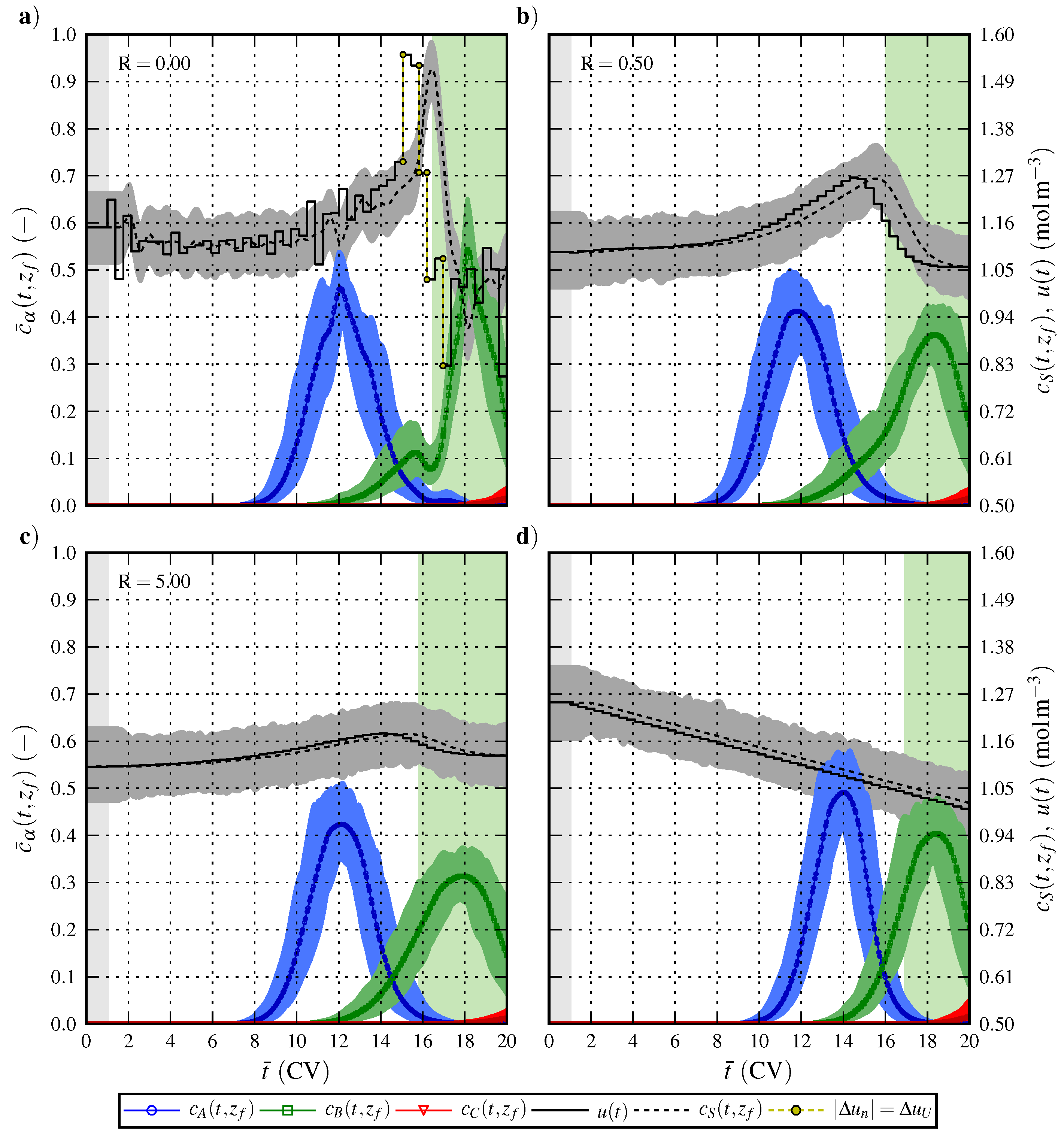
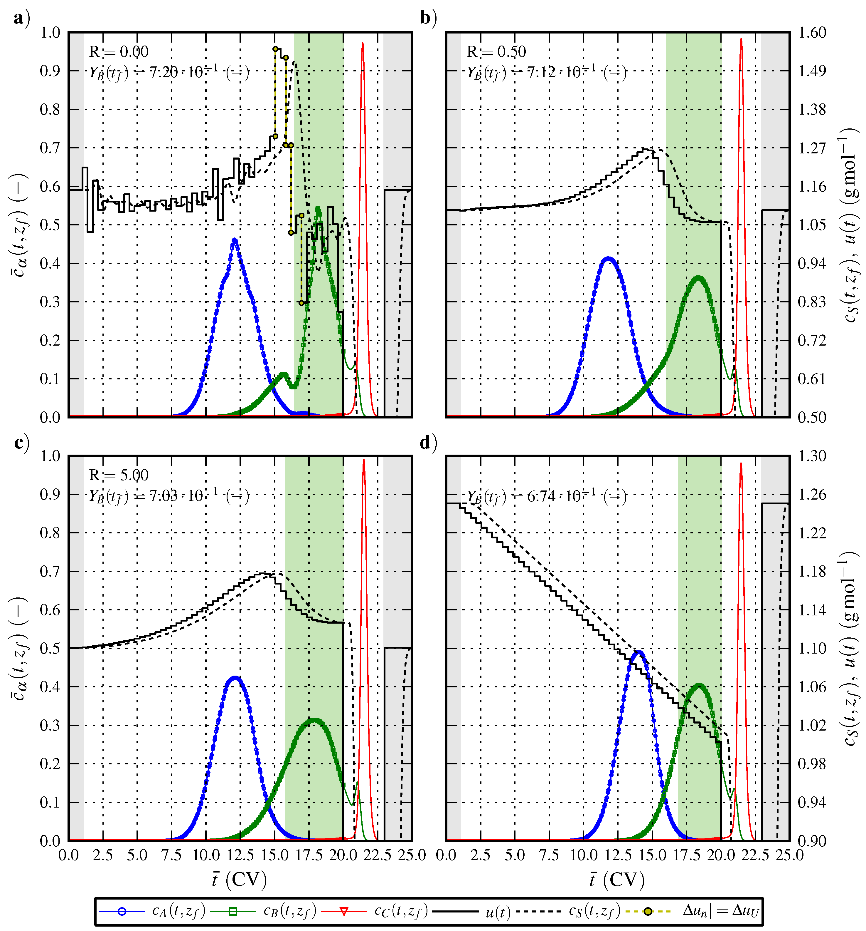
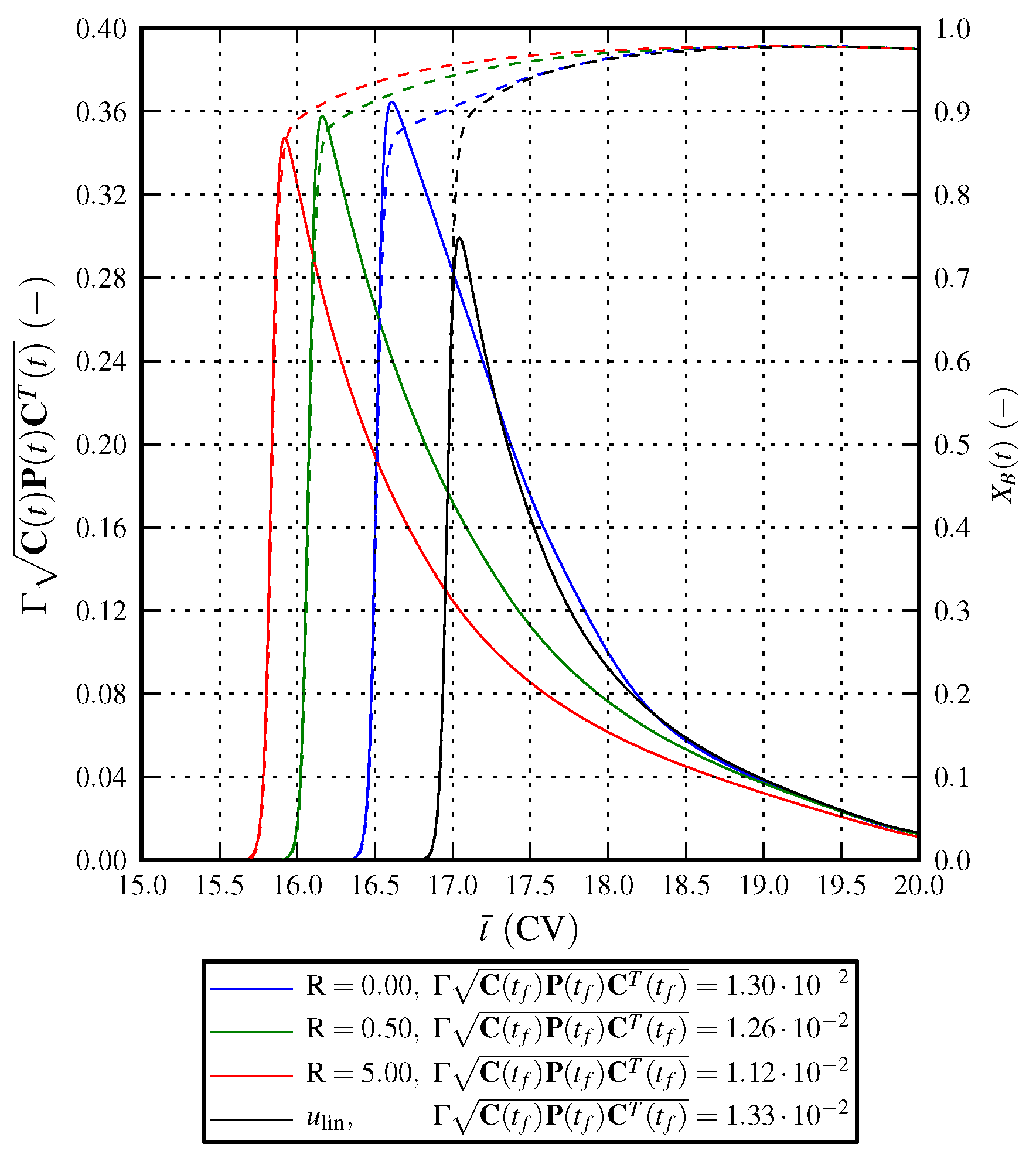
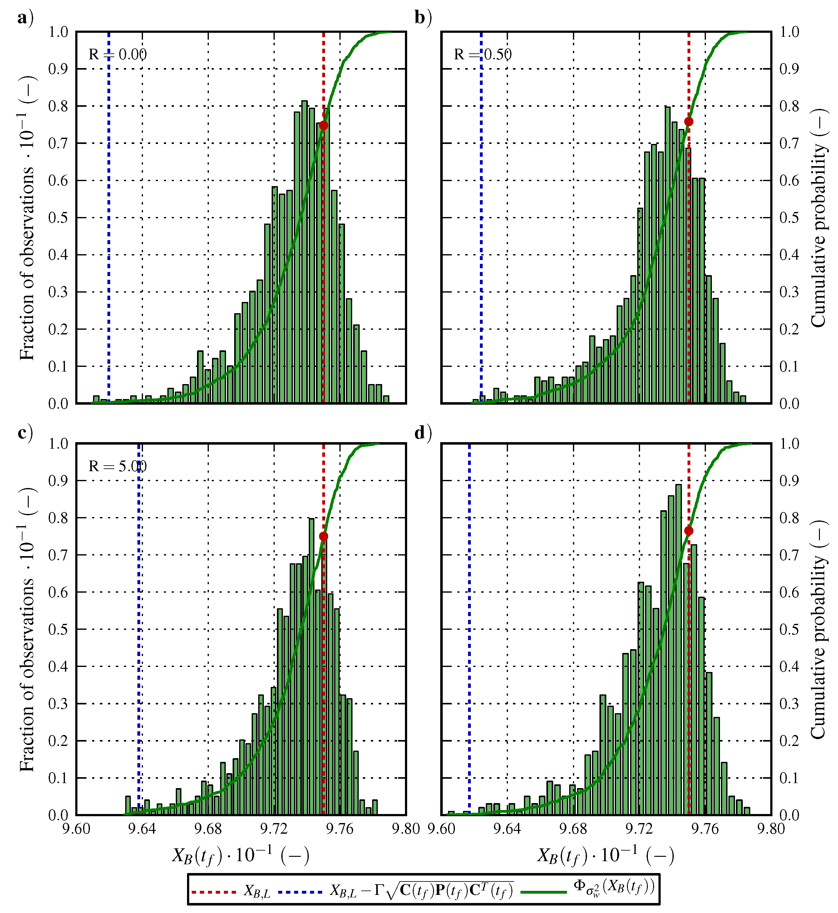
6.1. Optimal Control Strategy I—Nominal and Robustified Elution Trajectories in the Batch Elution Operation Mode

The nominal solution (i.e., without the presence of uncertainty) of the open-loop optimal control problem excluding the limit cycle criteria Equation (6) is computed over a fixed temporal horizon of $\forall \overline{t}\in [0.0,20.0]$. Here $\overline{t}=t\left(\dot{Q}{V}_c^{-1}\right)$ is the normalized time in column volumes (CV). The specifications in the optimization problem are $X_{B,L}=9.75\times {10}^{-1}(-)$, $\Delta u_U=2.5\times {10}^{-1}$, $u_L=5.0\times {10}^{-2}$ and $u_U=2.0$. Moreover, to reduce the state sensitivity of the optimal trajectories to control input uncertainties, we have introduced R as a key specification in the optimization problem. The resulting optimal state and control trajectories are depicted in Figure 6 and the associated optimization specifications are summarized in Table 3. The optimization and verification simulation results are practically identical. The initial control is constrained to be constant over the load and the subsequent wash horizon $[t_0,t_0+\Delta t_{\mathrm{load}}+\Delta t_{\mathrm{wash}}]$ where $\Delta t_{\mathrm{wash}}=1.0$ (CV). Although not considered in the open-loop optimal control problem, the control signal is prescribed a constant value of $1.0\times {10}^{-1}$$(\mathrm{moL}·{\mathrm{kg}}^{-1})$ during $2.5$ CV regeneration, in order to elute the most retained component, and the initial control, $u\left(t_0\right)$, is prescribed during the subsequently column re-equilibration period.

Figure 6. Optimal state and control trajectories, where $c_{\alpha }(t,z_f)$ and $\forall \alpha \in \{A,B,C\}$ is normalized with $[0.75,0.75,1.5]\times {10}^{-3}(\mathrm{moL}·{\mathrm{m}}^{-3})$, for $X_{B,L}=9.75\times {10}^{-1}(-)$ and $\mathrm{R}\in [0.0,5.0]$. Markers indicate the solution at the Radau collocation points and solid and dashed lines the corresponding simulated response. The shaded areas indicate the pooling interval endpoints, $[{\tau }_0,{\tau }_0+\Delta \tau ]$, and those of the initial load and wash and the terminal re-equilibration.

Figure 6. Optimal state and control trajectories, where $c_{\alpha }(t,z_f)$ and $\forall \alpha \in \{A,B,C\}$ is normalized with $[0.75,0.75,1.5]\times {10}^{-3}(\mathrm{moL}·{\mathrm{m}}^{-3})$, for $X_{B,L}=9.75\times {10}^{-1}(-)$ and $\mathrm{R}\in [0.0,5.0]$. Markers indicate the solution at the Radau collocation points and solid and dashed lines the corresponding simulated response. The shaded areas indicate the pooling interval endpoints, $[{\tau }_0,{\tau }_0+\Delta \tau ]$, and those of the initial load and wash and the terminal re-equilibration.

The optimal state and control trajectories illustrated in Figure 6 show a clear distinction in the system response generated with u and $u_{\mathrm{lin}}$, respectively. As expected from the generic HIC elution mode, $u_{\mathrm{lin}}$ and hence the optimal modifier concentration is strictly decreasing in $[t_{\mathrm{lin},0},t_f]$ in order to increase hydrophobicity, see Figure 6d. Governed by the individual component adsorption affinities, components $\alpha \in \{A,B,C\}$ are gradually separated as they traverse the column. It is noteworthy that parameterization Equation (30) for $u_{\mathrm{lin}}$ is augmented to the open-loop optimal control problem, however, a zero-order hold fit to that trajectory with $N_u=50$ segments (without affecting the state trajectories) is considered here for comparison purposes in the robustness assessment. Contrarily, the modifier concentration is freely controlled with the general elution trajectories, u, shown in Figure 6a–c. It is evident that the additional degrees of freedom introduced significantly promotes the recovery yield, $Y_B\left(t_f\right)$, of the intermediately eluting component B and that $Y_B\left(t_f\right)$ strictly increases as $\mathrm{R}\to 0$. Regardless of R, the solvent strength is gradually increasing until the lower optimal fractionation time, ${\tau }_0$, is reached. Moreover, at the onset of the fractionation interval, the slope of the elution trajectory changes sign, and the decreasing solvent strength causes the target component to desorb and ultimately to elute.

It is evident from analyzing Figure 7, where $X_B$ is depicted as a function of time for the nominal open-loop controlled trajectories, that the solution of Equation (11) yields that the inequality constraint imposed on target component purity is active, i.e., $X_B\left(t_f\right)=X_{B,L}$. More importantly, the associated back-off term, augmented to the purity inequality constraint in Equation (17), for ${\sigma }_w=5.0\%$ exhibits that neither of the optimal open-loop controls are robust at the given uncertainty level since $\Gamma \sqrt{\mathit{C}\left(t_f\right)\mathit{P}\left(t_f\right){\mathit{C}}^T\left(t_f\right)}>0$. This value corresponds to the worst-case purity to be expected and implies that the open-loop controlled system is unable to cope with control input variability experienced during nominal operation. Moreover, the back-off term trajectories pass through a maximum at the onset of the fractionation interval and subsequently decreases as $t\to t_f$. As expected, the terminal back-off value decreases with R for the general elution trajectories. It is however noteworthy that the linear elution trajectory is associated with the highest terminal back-off value. This is a key result, as the general elution trajectories not only outperforms the linear in terms of $Y_B\left(t_f\right)$ but also are inherently more robust.

Figure 7. Target component purity, $X_B\left(t\right)$, (dashed lines) and associated back-off term, $\Gamma \sqrt{\mathbf{C}\left(t\right)\mathbf{P}\left(t\right){\mathbf{C}}^T\left(t\right)}$, (solid lines) as a function of time for the nominal elution trajectories depicted in Figure 6.

Figure 7. Target component purity, $X_B\left(t\right)$, (dashed lines) and associated back-off term, $\Gamma \sqrt{\mathbf{C}\left(t\right)\mathbf{P}\left(t\right){\mathbf{C}}^T\left(t\right)}$, (solid lines) as a function of time for the nominal elution trajectories depicted in Figure 6.

The insight gained from analyzing Figure 7 clearly motivates the scope of this study, and the tools and methods developed here for solving the robust counterpart problem Equation (19). However, since the purity inequality constraint back-off term is determined by linearizing the dynamics around the nominal trajectories, it remains to assess the validity of that approximation. As discussed in Section 4.3, the validity of the robustification strategy is assessed by means of Monte Carlo simulations. A set of stochastic control signals, $\tilde{u}$, given by Equation (29) was generated by sampling a uniform distribution on the interval from $\pm {\sigma }_w$. For each case presented in Figure 6, $5.0\times {10}^3$ forward simulations were carried out for the uncertainty level of $5.0\%$. The resulting state and control trajectories are depicted in Figure 8. It is evident that the control signal variability has a direct affect on the individual components’ shape and retention time. Most critical is the significant fraction of impurity (component A and C) trajectories spanning inside the fractionation interval and causing degraded target component purity as a result. The corresponding probability distribution of the variability in $X_B\left(t_f\right)$ is depicted in Figure 9. This figure clearly strengthens the conclusion that the nominal open-loop controlled system is unable to cope with control input variability experienced during nominal operation. More importantly, it is evident that the deterministic back-off value corresponds to a high degree with the worst-case observations of the stochastic distribution of $X_B\left(t_f\right)$, and consequently, the linearized approximation Equation (13) is valid for the uncertainty level considered.

Figure 8. State and control trajectories generated with the set of stochastic control signals, $\tilde{u}$, sampled from a uniform distribution with the uncertainty level ${\sigma }_w=5.0\%$. Markers indicate the nominal optimal solution at the Radau collocation points and solid and dashed lines the corresponding simulated response.

Figure 8. State and control trajectories generated with the set of stochastic control signals, $\tilde{u}$, sampled from a uniform distribution with the uncertainty level ${\sigma }_w=5.0\%$. Markers indicate the nominal optimal solution at the Radau collocation points and solid and dashed lines the corresponding simulated response.

Figure 9. Probability distribution of the variability in $X_B\left(t_f\right)$ generated with the set of stochastic control signals, $\tilde{u}$, sampled from a uniform distribution with the uncertainty level ${\sigma }_w=5.0\%$. The dashed lines indicate the lower purity constraint, $X_{B,L}$, and the deterministic worst-case purity, $X_{B,L}-\Gamma \sqrt{\mathit{C}\left(t_f\right)\mathit{P}\left(t_f\right){\mathit{C}}^T\left(t_f\right)}$. The solid line indicates the cumulative probability, ${\Phi }_{{\sigma }_w^2}\left(X_B\left(t_f\right)\right)$.

Figure 9. Probability distribution of the variability in $X_B\left(t_f\right)$ generated with the set of stochastic control signals, $\tilde{u}$, sampled from a uniform distribution with the uncertainty level ${\sigma }_w=5.0\%$. The dashed lines indicate the lower purity constraint, $X_{B,L}$, and the deterministic worst-case purity, $X_{B,L}-\Gamma \sqrt{\mathit{C}\left(t_f\right)\mathit{P}\left(t_f\right){\mathit{C}}^T\left(t_f\right)}$. The solid line indicates the cumulative probability, ${\Phi }_{{\sigma }_w^2}\left(X_B\left(t_f\right)\right)$.

As discussed in Section 1.3, introducing more robustness always give rise to a performance decrease. Hence, the robustification of the open-loop controlled system implies compromising high penalties on the change in the zero-order hold control, yielding optimal solutions with low sensitivity to uncertainty, however, to the expense of an overall lower performance. This is solely the main reason for introducing R as an optimization variable in the upper-level robust counterpart problem Equation (19a)–(19d). It is however noteworthy that neither the stochastic nor the deterministic worst-case purity depicted in Figure 9 is valid for any other open-loop control input associated with a different lower purity requirement than of $X_{B,L}=9.75\times {10}^{-1}$. Therefore, in order to find the optimal robustified controls associated with the nominal open-loop trajectories depicted in Figure 6, an iterative approach was adopted. Hence, this iterative approach implies solving the feasibility problem to the robust counterpart problem Equation (19) when keeping R fixed. The resulting robustified state and control trajectories are depicted in Figure 10 together with their nominal trajectories for comparison purposes.

It is evident from analyzing Figure 10 that the onset of the fractionation interval is slightly shifted towards higher elution volumes for all cases studied. The largest discrepancies between the nominal and the robustified general controls is seen in the temporal region for $t>{\tau }_0$. As a consequence, the state trajectory for component A is not affected to a high degree, whereas the state trajectory for the target component B is significantly affected. Moreover, the nominal linear control differ significantly from its robust counterpart both in terms of the initial level and the slope, and consequently, all state trajectories are affected. It is noteworthy that the performance increase in terms of $Y_B\left(t_f\right)$ for u compared to $u_{\mathrm{lin}}$ is even higher for the robustified solutions than for that obtained with the nominal solutions. This can be explained by the lower back-off value associated with the general trajectories. Specifically, the lower purity constraint augmented with the safety margin, $X_{B,L}+\Gamma \sqrt{\mathit{C}\left(t_f\right)\mathit{P}\left(t_f\right){\mathit{C}}^T\left(t_f\right)}$, is $9.821\times {10}^{-1}$ for $\mathrm{R}=0.0$ and $9.836\times {10}^{-1}$ for $u_{\mathrm{lin}}$. Finally, for the HIC separation case considered in this paper, the target component yield governed by the robustified general elution trajectories is strictly decreasing with the penalty on the change in the zero-order hold control, and consequently, the solution of the robust counterpart problem Equation (19) is obtained for $\mathrm{R}=0.0$, see Figure 10a. This was not expected a priori since the unpenalized input control is associated with the largest purity inequality constraint safety margin. However, the case considered in this study clearly demonstrates the applicability of the tools and methods developed here for formulating and solving the robust counterpart problem.

Figure 10. Nominal and robustified state and control trajectories. Markers indicate the robustified solution at the Radau collocation points and solid and dashed lines the corresponding simulated response. The light colored state and control trajectories indicate the nominal solution.

Figure 10. Nominal and robustified state and control trajectories. Markers indicate the robustified solution at the Radau collocation points and solid and dashed lines the corresponding simulated response. The light colored state and control trajectories indicate the nominal solution.

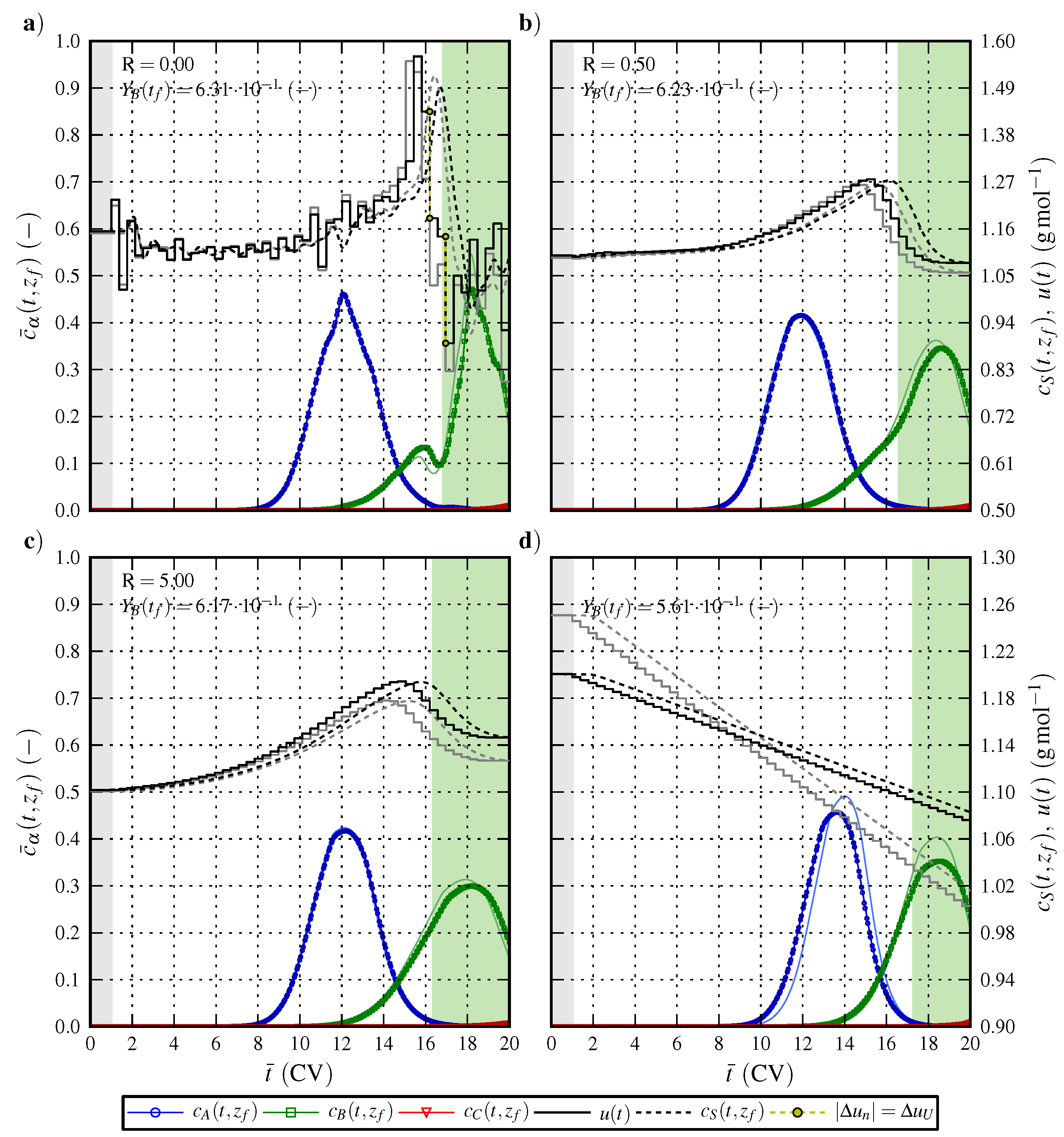
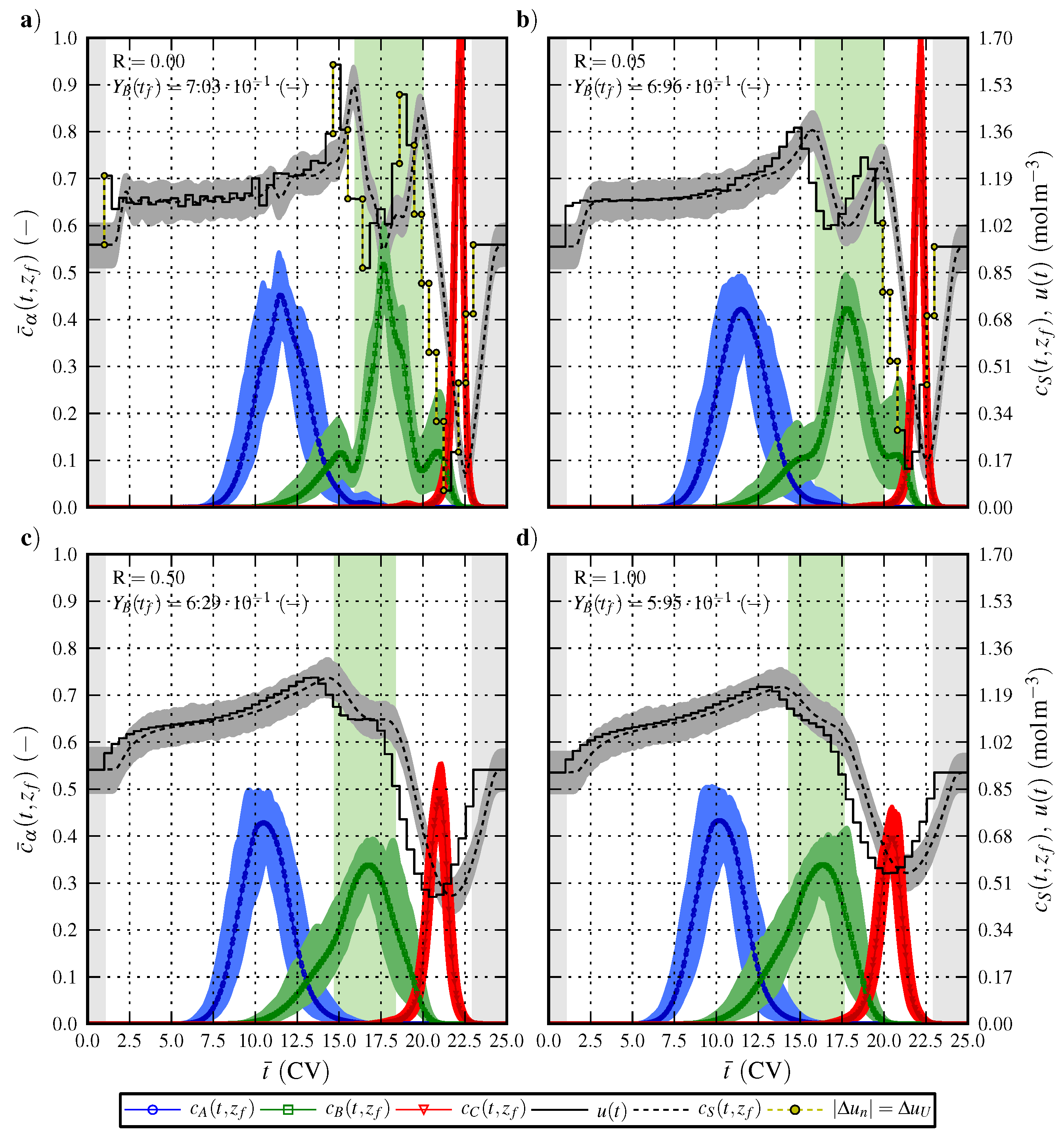
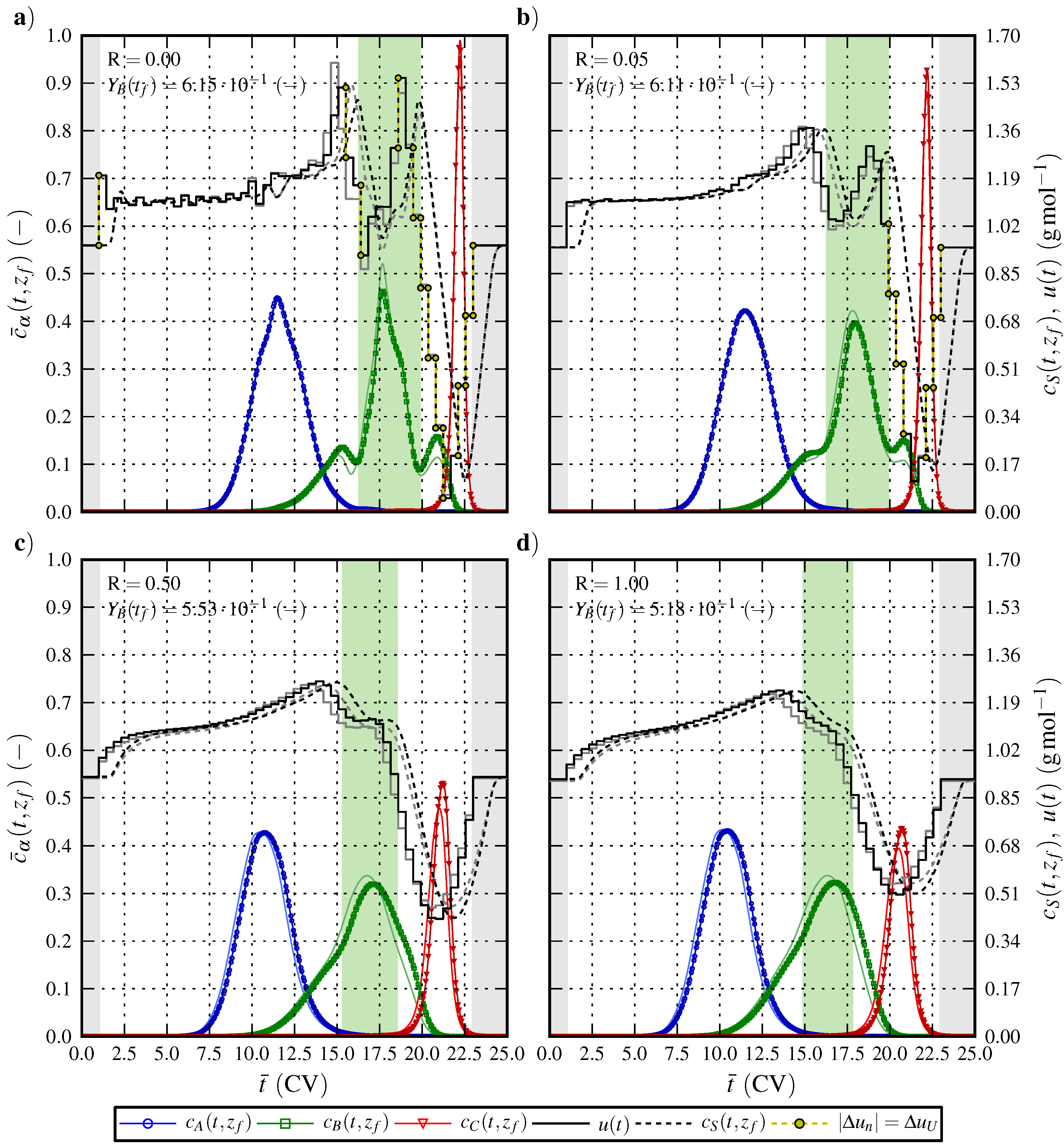
6.2. Optimal Control Strategy II—Nominal and Robustified Elution Trajectories in the Cyclic-Steady-State Operation Mode

So far, we have shown the optimal open-loop and the robustified elution trajectories for the control strategy excluding the limit cycle criteria. This section is therefore devoted to demonstrate robust optimal control of the comprehensive cyclic-steady-state formalism. As outlined in Section 4.1, computation of CSS solutions over the temporal horizon $t\in [t_0,t_f]$ requires that open-loop optimal control problem Equation (11) is augmented with the limit cycle criteria Equation (6) governing that the state at the initial time is retained at the end of the cycle. The resulting nominal state and control trajectories that conform to the periodic boundary condition over a fixed temporal horizon of $\forall \overline{t}\in [0.0,25.0]$ are displayed in Figure 11 and the associated optimization specifications are summarized in Table 4. Here, the initial control, $u\left(t_0\right)$, is constrained to be constant over the load and the subsequent wash horizon $[t_0,t_0+\Delta t_{\mathrm{load}}+\Delta t_{\mathrm{wash}}]$. Moreover, the control in the final re-equilibration horizon $[t_f-\Delta t_{\mathrm{eq}},t_f]$, where $\Delta t_{\mathrm{eq}}=2.0$ (CV), is prescribed the constant value of $u\left(t_0\right)$ through the limit cycle criteria in Equation (6d).

Figure 11. State and control trajectories generated for $X_{B,L}=9.75\times {10}^{-1}(-)$ and $\mathrm{R}\in [0.0,1.0]$. The set of stochastic control signals, $\tilde{u}$, was sampled from a uniform distribution with the uncertainty level ${\sigma }_w=5.0\%$. Markers indicate nominal state and control trajectories that conform to the cyclic-steady state criteria Equation (6) over the temporal horizon $[t_0,t_f]$ at the Radau collocation points and solid and dashed lines the corresponding simulated response.

Figure 11. State and control trajectories generated for $X_{B,L}=9.75\times {10}^{-1}(-)$ and $\mathrm{R}\in [0.0,1.0]$. The set of stochastic control signals, $\tilde{u}$, was sampled from a uniform distribution with the uncertainty level ${\sigma }_w=5.0\%$. Markers indicate nominal state and control trajectories that conform to the cyclic-steady state criteria Equation (6) over the temporal horizon $[t_0,t_f]$ at the Radau collocation points and solid and dashed lines the corresponding simulated response.

In accordance with the optimal open-loop controlled trajectories depicted in Figure 6, the solvent strength is gradually increasing until the lower optimal fractionation time, ${\tau }_0$, is reached. For $\mathrm{R}>1.0$, the slope of the control trajectory changes sign within the fractionation interval in order to prevent the most retained component to desorb. Moreover, at the upper fractionation interval endpoint, the control trajectory drops drastically in order to completely elute component C, and to fulfill Equation (6a), before returning to the initial control level. For these reasons, the upper endpoint of the fractionation interval, ${\tau }_0+\Delta \tau$, do not coincide with the that of the temporal horizon, as was the case for the optimal control trajectories shown in Figure 6. It is also evident from Figure 11 that the penalty on $\Delta u_n$ significantly affect the state and control trajectories, due to the large difference of the maximum and minimum values of $u_n$, and that the target component recovery yield strictly increases as $\mathrm{R}\to 0$.

The deterministic back-off terms determined by linearizing the system dynamics around the nominal trajectories that conform to the CSS criteria are shown in Figure 12. The $\Gamma \sqrt{\mathbf{C}\left(t\right)\mathbf{P}\left(t\right){\mathbf{C}}^T\left(t\right)}$ trajectories exhibit analogous temporal behavior as for those depicted in Figure 7. Likewise, the terminal back-off value decreases with R. As the purity inequality constraint is active, and terminal back-off value is larger than zero $\forall \mathrm{R}\in [0.0,1.0]$, the open-loop controlled system is unable to cope with control input variability experienced during nominal operation. The validity of the deterministic worst-case purity was also here assessed by means of Monte Carlo simulations, as previously outlined in Section 6.1. The probability distribution of the variability in $X_B\left(t_f\right)$ depicted in Figure 13 is determined by the state trajectories subject to the set of stochastic controls, $\tilde{u}$, shown in Figure 11. The deterministic terminal back-off value corresponds to a high degree with the worst-case observations of the stochastic distribution of $X_B\left(t_f\right)$ shown in Figure 13, and consequently, the linearized approximation Equation (13) is valid for the uncertainty level considered and can therefore safely be exploited in the robustification approach.

Figure 12. Target component purity, $X_B\left(t\right)$, (dashed lines) and associated back-off term, $\Gamma \sqrt{\mathbf{C}\left(t\right)\mathbf{P}\left(t\right){\mathbf{C}}^T\left(t\right)}$, (solid lines) as a function of time for the nominal elution trajectories depicted in Figure 11.

Figure 12. Target component purity, $X_B\left(t\right)$, (dashed lines) and associated back-off term, $\Gamma \sqrt{\mathbf{C}\left(t\right)\mathbf{P}\left(t\right){\mathbf{C}}^T\left(t\right)}$, (solid lines) as a function of time for the nominal elution trajectories depicted in Figure 11.

Figure 13. Probability distribution of the variability in $X_B\left(t_f\right)$ generated with the set of stochastic control signals, $\tilde{u}$, sampled from a uniform distribution with the uncertainty level ${\sigma }_w=5.0\%$. The dashed lines indicate the lower purity constraint, $X_{B,L}$, and the deterministic worst-case purity, $X_{B,L}-\Gamma \sqrt{\mathit{C}\left(t_f\right)\mathit{P}\left(t_f\right){\mathit{C}}^T\left(t_f\right)}$. The solid line indicates the cumulative probability, ${\Phi }_{{\sigma }_w^2}\left(X_B\left(t_f\right)\right)$.

Figure 13. Probability distribution of the variability in $X_B\left(t_f\right)$ generated with the set of stochastic control signals, $\tilde{u}$, sampled from a uniform distribution with the uncertainty level ${\sigma }_w=5.0\%$. The dashed lines indicate the lower purity constraint, $X_{B,L}$, and the deterministic worst-case purity, $X_{B,L}-\Gamma \sqrt{\mathit{C}\left(t_f\right)\mathit{P}\left(t_f\right){\mathit{C}}^T\left(t_f\right)}$. The solid line indicates the cumulative probability, ${\Phi }_{{\sigma }_w^2}\left(X_B\left(t_f\right)\right)$.

The resulting robustified control trajectories, from solving the feasibility problem to the robust counterpart problem Equation (19) when keeping R fixed, are depicted in Figure 14 together with their nominal trajectories for comparison purposes. Again, the largest discrepancy between the nominal and robustified controls are seen in the temporal region around the fractionation interval and ${\tau }_0$ is slightly shifted towards larger elution volumes, whereas $\Delta \tau$ is unchanged. It is also evident that the initial control levels almost coincide. Consequently, the state trajectories for component A and C is not affected to a high degree. Hence, in order to meet the robustified purity inequality constraint augmented with the back-off term Equation (17), only the state trajectory of component B is slightly modified. Here, $X_{B,L}+\Gamma \sqrt{\mathit{C}\left(t_f\right)\mathit{P}\left(t_f\right){\mathit{C}}^T\left(t_f\right)}$ is $[9.815,9.814,9.806,9.803]\times {10}^{-1}$ for $\mathrm{R}\in [0.0,0.05,0.5,1.0]$. Hence, there is only a moderate increase in the terminal back-off value as $\mathrm{R}\to 0$, and consequently, the solution of the robust counterpart problem Equation (19) is obtained for the unpenalized control, see Figure 14a.

Figure 14. Nominal and robust cyclic-steady-state elution profiles for $\mathrm{R}\in [0.0,1.0]$. Markers indicate the robustified solution at the Radau collocation points and solid and dashed lines the corresponding simulated response. The light colored state and control trajectories indicate the nominal solution.

Figure 14. Nominal and robust cyclic-steady-state elution profiles for $\mathrm{R}\in [0.0,1.0]$. Markers indicate the robustified solution at the Radau collocation points and solid and dashed lines the corresponding simulated response. The light colored state and control trajectories indicate the nominal solution.

7. Conclusions

External process disturbances are inevitably present and the robustness of the open-loop controlled system with respect to CPP uncertainties, e.g., guaranteeing that QCA requirements are not violated, is of the highest importance in biopharmaceutical process industry. Especially, the solution of the open-loop optimal control problem will yield trajectories that lie on the boundary of the feasible region, and consequently, the open-loop controlled system is unable to cope with control input variability experienced during nominal operation. This paper is therefore concerned with extending the open-loop optimal control problem, constrained by a nonlinear dynamic system governed by PDEs, with its robust counterpart formulation. However, there is a drastic increase in computational complexity while moving from the nominal problem to its robust counterpart. To efficiently and accurately generate optimal elution trajectories in the presence of uncertainty we considered a deterministic robust formulation, that employs a linearization of the uncertainty set, for dynamic systems based on Lyapunov differential equations. While the approximate robust approach is computationally tractable for medium-scale ODE-constrained DOPs, it is not for the original PDE-constrained DOP considered here. One of the main contributions of this paper is therefore the established methodology and the computationally efficient framework for robust optimal control of batch chromatographic separation processes. It is however noteworthy that the generic methods and tools developed here are applicable to any large-scale optimal control problem constrained by PDEs.

Computational tractability was obtained by casting the robust counterpart problem in the frame of bilevel optimal control where the upper level concerns forward simulation of the Lyapunov differential equations and the system dynamics, and the nominal DOP augmented with the robustified inequality constraint margin is considered in the lower level. The lower-level DOP constrained by the system dynamics is transcribed into a sparse NLP using direct collocation, which is then solved by IPOPT supplied with the first- and second-order derivatives of the NLP functions computed using CasADi’s algorithmic differentiation while preserving sparsity. The adopted decomposition strategy thereby avoids the full simultaneous discretization of the Lyapunov states, which are too numerous to be treated with direct collocation. However, the coupled system of the Lyapunov differential equations and the process model ODEs significantly increased the problem dimension of the upper level. In order to reduce the over-all execution time it was crucial that the sparsity is used during the simulation and that the structure is used during the assembly of the partial derivatives. This was realized by extending PyFMI to support adding additional equations to the original problem of simulating an FMU as well as to handle the sparse representation of the Jacobian together with the connection to the sparse solver in CVode. Finally, in order to reduce the state sensitivity of the optimal trajectories to control input uncertainties, we have introduced an optimization variable in the upper level that penalizes the change in the zero-order hold control. This parameter influence the smoothness of the control and consequently enhance the robustness, however, to the expense of an overall lower performance.

The advantages of the deterministic robustification methodology were illustrated through the solution of a specific challenging ternary complex mixture separation problem of insulin analogs, with the intermediately eluting component as the target, by hydrophobic interaction chromatography. Moreover, two inherently different optimal control strategies were considered and the discrepancy lies in whether robust counterpart problem is augmented with the cyclic-steady-state criteria or not. The deterministic back-off term, determined by linearizing the system around the nominal open-loop controlled trajectories, for both control strategies showed good agreement with the worst-case observations of the stochastic distribution of purity obtained by means of Monte Carlo simulations. A common trend is that the terminal back-off term value strictly decreased with the value of the penalty on change in the zero-order hold control, hence, yielding solutions with lower sensitivity to control variability.

A key result of this study is that the general elution trajectories nonconforming to CSS criteria outperformed the conventional linear trajectories both in terms of recovery yield and robustness. Especially, the performance increase obtained for the robustified trajectories was even more pronounced than that obtained with the open-loop controlled trajectories. This is due to the lower back-off value associated with the general trajectories which allow for the fractionation interval to span over a wider temporal horizon. Moreover, the solution of the robust counterpart problem was obtained for the unpenalized control input. Likewise, the robustified solution conforming to the CSS criteria is also obtained for the unpenalized control input although associated with the largest purity inequality constraint safety margin. This is a result of the moderate increase in the value of the terminal back-off as the penalty on the change in the zero-order hold control goes to zero.

Several interesting paths may be taken to further develop the robustified methodology presented in this paper. Especially, it is not certain that the unpenalized control gives the optimal robustified solution for a different ternary separation problem or a different chromatographic separation mode (e.g., reverse phase and ion exchange). It also remains to assess the robustness of the nominal multi-objective optimal control problem, including the production rate and the recovery concentration, as well as considering variability in the feed concentration.

References

1. Ündey, C.; Ertunç, S.; Mistretta, T.; Looze, B. Applied advanced process analytics in biopharmaceutical manufacturing: Challenges and prospects in real-time monitoring and control. J. Process Control 2010, 20, 1009–1018. [Google Scholar] [CrossRef]
2. Jungbauer, A. Chromatographic media for bioseparation. J. Chromatogr. A 2005, 1065, 3–12. [Google Scholar] [CrossRef] [PubMed]
3. Wisniewski, E.; Boschetti, E.; Jungbauer, A. Biotechnology and biopharmaceutical manufacturing, processing, and preservation. In Drug Manufacturing Technology Series, 1st ed.; Avis, K.E., Wu, V.L., Eds.; Interpharm Press, Inc.: Buffalo Grove, IL, USA, 1996; Volume 2. [Google Scholar]
4. Department of Health and Human Services U.S. Food and Drug Administration. Pharmaceutical cGMPs for the 21st Century: A Risk-based Approach; U.S. Food and Drug Administration: Silver Spring, MD, USA, 2004.
5. Chirino, A.; Mire-Sluis, A. Characteristics biological products and assessing comparability following manufacturing changes. Nat. Biotechnol. 2004, 22, 1383–1391. [Google Scholar] [CrossRef] [PubMed]
6. Rathore, A.S.; Yu, M.; Yeboah, S.; Sharma, A. Case study and application of process analytical technology (PAT) towards bioprocessing: Use of on-line high-performance liquid chromatography (HPLC) for making real-time pooling decisions for process chromatography. Biotechnol. Bioeng. 2008, 100, 306–316. [Google Scholar] [CrossRef] [PubMed]
7. Close, E.J.; Salm, J.R.; Bracewell, D.G.; Sorensen, E. A model based approach for identifying robust operating conditions for industrial chromatography with process variability. Chem. Eng. Sci. 2014, 116, 284–295. [Google Scholar] [CrossRef]
8. Jiang, C.; Flansburg, L.; Ghose, S.; Jorjorian, P.; Shukla, A.A. Defining process design space for a hydrophobic interaction chromatography (HIC) purification step: Application of quality by design (QbD) principles. Biotechnol. Bioeng. 2010, 107, 985–997. [Google Scholar] [CrossRef] [PubMed]
9. Harms, J.; Wang, X.; Kim, T.; Yang, X.; Rathore, A.S. Defining process design space for biotech products: Case study of pichia pastoris fermentation. Biotechnol. Prog. 2008, 24, 655–662. [Google Scholar] [CrossRef] [PubMed]
10. Rathore, A.; Winkle, H. Quality by design for biopharmaceuticals. Nat. Biotechnol. 2009, 27, 26–34. [Google Scholar] [CrossRef] [PubMed]
11. Mota, J.P.B.; Araújo, J.M.M.; Rodrigues, R.C.R. Optimal design of simulated moving-bed processes under flow rate uncertainty. AIChE J. 2007, 53, 2630–2642. [Google Scholar] [CrossRef]
12. Degerman, M.; Westerberg, K.; Nilsson, B. A model-based approach to determine the design space of preparative chromatography. Chem. Eng. Technol. 2009, 32, 1195–1202. [Google Scholar] [CrossRef]
13. Westerberg, K.; Broberg Hansen, E.; Degerman, M.; Budde Hansen, T.; Nilsson, B. Model-based process challenge of an industrial ion-exchange chromatography step. Chem. Eng. Technol. 2012, 35, 183–190. [Google Scholar] [CrossRef]
14. Borg, N.; Westerberg, K.; Andersson, N.; von Lieres, E.; Nilsson, B. Effects of uncertainties in experimental conditions on the estimation of adsorption model parameters in preparative chromatography. Comput. Chem. Eng. 2013, 55, 148–157. [Google Scholar] [CrossRef]
15. Snyder, L.R.; Dolan, J.W. High-Performance Gradient Elution: The Practical Application of the Linear-Solvent-Strength Model; John Wiley & Sons, Inc.: Hoboken, NJ, USA, 2007. [Google Scholar]
16. Sreedhar, B.; Wagler, A.; Kaspereit, M.; Seidel-Morgenstern, A. Optimal cut-times finding strategies for collecting a target component from overloaded elution chromatograms. Comput. Chem. Eng. 2013, 49, 158–169. [Google Scholar] [CrossRef]
17. Gritti, F.; Guiochon, G. The distortion of gradient profiles in reversed-phase liquid chromatography. J. Chromatogr. A 2014, 1340, 50–58. [Google Scholar] [CrossRef] [PubMed]
18. Tarafder, A.; Aumann, L.; Müller-Späth, T.; Morbidelli, M. Improvement of an overloaded, multi-component, solvent gradient bioseparation through multiobjective optimization. J. Chromatogr. A 2007, 1167, 42–53. [Google Scholar] [CrossRef] [PubMed]
19. Damtew, A.; Sreedhar, B.; Seidel-Morgenstern, A. Evaluation of the potential of nonlinear gradients for separating a ternary mixture. J. Chromatogr. A 2009, 1216, 5355–5364. [Google Scholar] [CrossRef] [PubMed]
20. Nikitas, P.; Pappa-Louisi, A.; Papachristos, K. Optimisation technique for stepwise gradient elution in reversed-phase liquid chromatography. J. Chromatogr. A 2004, 1033, 283–289. [Google Scholar] [CrossRef] [PubMed]
21. Holmqvist, A.; Magnusson, F. Open-loop optimal control of batch chromatographic separation processes using direct collocation. J. Process Control 2015. submitted for publication. [Google Scholar]
22. Holmqvist, A.; Magnusson, F.; Nilsson, B. Dynamic  multi-objective  optimization  of batch chromatographic separation processes. Computer Aided Chemical Engineering 2015, Volume 37, 815–820. [Google Scholar]
23. ICH Harmonised Tripartite Guideline. Pharmaceutical Development Q8(R2), Annex to Pharmaceutical Development, Step 4, August 2009. Available online: http://www.ich.org/products/guidelines/quality/article/quality-guidelines.html (accessed on 10 July 2015).
24. Ben-Tal, A.; El Ghaoui, L.; Nemirovski, A. Robust Optimization; Daubechies, I., Weinan, E., Lenstra, J.K., Süli, E., Eds.; Princeton University Press: Princeton, NJ, USA, 2009. [Google Scholar]
25. Schmidt-Traub, H.; Schulte, M.; Seidel-Morgenstern, A. Preparative Chromatography, 2nd ed.; Wiley-VCH: Weinheim, Germany, 2012. [Google Scholar]
26. Lienqueo, M.E.; Mahn, A.; Salgado, J.C.; Asenjo, J.A. Current insights on protein behaviour in hydrophobic interaction chromatography. J. Chromatogr. B 2007, 849, 53–68. [Google Scholar] [CrossRef] [PubMed]
27. Mahn, A.; Lienqueo, M.E.; Asenjo, J.A. Optimal operation conditions for protein separation in hydrophobic interaction chromatography. J. Chromatogr. B 2007, 849, 236–242. [Google Scholar] [CrossRef] [PubMed]
28. Biegler, L.T.; Ghattas, O.; Heinkenschloss, M.; van Bloemen Waanders, B. Large-scale PDE-constrained optimization. In Lecture Notes in Computational Science and Engineering; Barth, T.J., Griebel, M., Keyes, D.E., Nieminen, R.M., Roose, D., Schlick, T., Eds.; Springer: Berlin, Germany, 2003; Volume 30. [Google Scholar]
29. Wendl, S.; Pesch, H.; Rund, A. On a state-constrained PDE optimal control. In Recent Advances in Optimization and its Applications in Engineering; Diehl, M., Glineur, F., Jarlebring, E., Michiels, W., Eds.; Springer: Berlin, Germany, 2010; pp. 429–438. [Google Scholar]
30. Herzog, R.; Kunisch, K. Algorithms for PDE-constrained optimization. GAMM-Mitteilungen 2010, 33, 163–176. [Google Scholar] [CrossRef]
31. Biegler, L.T. Nonlinear Programming: Concepts, Algorithms, and Applications to Chemical Processes; Society for Industrial and Applied Mathematics: Philadelphia, PA, USA, 2010. [Google Scholar]
32. Betts, J. Practical Methods for Optimal Control and Estimation Using Nonlinear Programming, 2nd ed.; SIAM’s Advances in Design and Control; Society for Industrial and Applied Mathematics: Philadelphia, PA, USA, 2010. [Google Scholar]
33. Davis, M.E. Numerical Methods and Modeling for Chemical Engineers, 1st ed.; John Wiley & Sons, Inc.: New York, NY, USA, 1984. [Google Scholar]
34. Schiesser, W.E. The Numerical Method of Lines: Integration of Partial Differential Equations, 1st ed.; Academic Press: San Diago, CA, USA, 1991. [Google Scholar]
35. Gao, W.; Engell, S. Iterative set-point optimization of batch chromatography. Comput. Chem. Eng. 2005, 29, 1401–1409. [Google Scholar] [CrossRef]
36. Dünnebier, G.; Engell, S.; Epping, A.; Hanisch, F.; Jupke, A.; Klatt, K.U.; Schmidt-Traub, H. Model-based control of batch chromatography. AIChE J. 2001, 47, 2493–2502. [Google Scholar] [CrossRef]
37. Kawajiri, Y.; Biegler, L.T. Optimization strategies for simulated moving bed and PowerFeed processes. AIChE J. 2006, 52, 1343–1350. [Google Scholar] [CrossRef]
38. Nagrath, D.; Messac, A.; Bequette, B.W.; Cramer, S.M. A hybrid model framework for the optimization of preparative chromatographic processes. Biotechnol. Prog. 2004, 20, 162–178. [Google Scholar] [CrossRef] [PubMed]
39. Sreedhar, B.; Damtew, A.; Seidel-Morgenstern, A. Theoretical study of preparative chromatography using closed-loop recycling with an initial gradient. J. Chromatogr. A 2009, 1216, 4976–4988. [Google Scholar] [CrossRef] [PubMed]
40. Jiang, G.S.; Shu, C.W. Efficient implementation of weighted ENO schemes. J. Comput. Phys. 1996, 126, 202–228. [Google Scholar] [CrossRef]
41. Shu, C.W. Essentially non-oscillatory and weighted essentially non-oscillatory schemes for hyperbolic conservation laws. In Advanced Numerical Approximation of Nonlinear Hyperbolic Equations; Quarteroni, A., Ed.; Springer: Berlin, Germany, 1998; Volume 1697, pp. 325–432. [Google Scholar]
42. John, V.; Novo, J. On (essentially) non-oscillatory discretizations of evolutionary convection–diffusion equations. J. Comput. Phys. 2012, 231, 1570–1586. [Google Scholar] [CrossRef]
43. Wächter, A.; Biegler, L.T. On the implementation of an interior-point filter line-search algorithm for large-scale nonlinear programming. Math. Programm. 2006, 106, 25–57. [Google Scholar] [CrossRef]
44. Griewank, A. Evaluating Derivatives: Principles and Techniques of Algorithmic Differentiation; Society for Industrial and Applied Mathematics: Philadelphia, PA, USA, 2000. [Google Scholar]
45. Püttmann, A.; Schnittert, S.; Naumann, U.; von Lieres, E. Fast and accurate parameter sensitivities for the general rate model of column liquid chromatography. Comput. Chem. Eng. 2013, 56, 46–57. [Google Scholar] [CrossRef]
46. Sahinidis, N.V. Optimization under uncertainty: State-of-the-art and opportunities. Comput. Chem. Eng. 2004, 28, 971–983. [Google Scholar] [CrossRef]
47. Mitra, K. Multiobjective optimization of an industrial grinding operation under uncertainty. Chem. Eng. Sci. 2009, 64, 5043–5056. [Google Scholar] [CrossRef]
48. Pinto, J.C. On the costs of parameter uncertainties. Effects of parameter uncertainties during optimization and design of experiments. Chem. Eng. Sci. 1998, 53, 2029–2040. [Google Scholar]
49. Logist, F.; Houska, B.; Diehl, M.; van Impe, J.F. Robust multi-objective optimal control of uncertain (bio)chemical processes. Chem. Eng. Sci. 2011, 66, 4670–4682. [Google Scholar] [CrossRef]
50. Houska, B.; Diehl, M. Nonlinear robust optimization of uncertainty affine dynamic systems under the L-infinity norm. In Proceedings of the IEEE International Symposium on Computer-Aided Control System Design (CACSD), Yokohama, Japan, 8–10 September 2010; pp. 1091–1096.
51. Houska, B.; Logist, F.; Impe, J.V.; Diehl, M. Robust optimization of nonlinear dynamic systems with application to a jacketed tubular reactor. J. Process Control 2012, 22, 1152–1160. [Google Scholar] [CrossRef]
52. Klatt, K.U.; Hanisch, F.; Dünnebier, G.; Engell, S. Model-based optimization and control of chromatographic processes. Comput. Chem. Eng. 2000, 24, 1119–1126. [Google Scholar] [CrossRef]
53. Shan, Y.; Seidel-Morgenstern, A. Optimization of gradient elution conditions in multicomponent preparative liquid chromatography. J. Chromatogr. A 2005, 1093, 47–58. [Google Scholar] [CrossRef] [PubMed]
54. Hansen, S.K.; Skibsted, E.; Staby, A.; Hubbuch, J. A label-free methodology for selective protein quantification by means of absorption measurements. Biotechnol. Bioeng. 2011, 108, 2661–2669. [Google Scholar] [CrossRef] [PubMed]
55. Sherwood, T.K.; Pigford, R.L.; Wilke, C.R. Mass Transfer; McGraw-Hill: New York, NY, USA, 1975. [Google Scholar]
56. Mollerup, J.M. A review of the thermodynamics of protein association to ligands, protein adsorption, and adsorption isotherms. Chem. Eng. Technol. 2008, 31, 864–874. [Google Scholar] [CrossRef]
57. Forssén, P.; Arnell, R.; Fornstedt, T. An improved algorithm for solving inverse problems in liquid chromatography. Comput. Chem. Eng. 2006, 30, 1381–1391. [Google Scholar] [CrossRef]
58. Cornel, J.; Tarafder, A.; Katsuo, S.; Mazzotti, M. The direct inverse method: A novel approach to estimate adsorption isotherm parameters. J. Chromatogr. A 2010, 1217, 1934–1941. [Google Scholar] [CrossRef] [PubMed]
59. Hahn, T.; Sommer, A.; Osberghaus, A.; Heuveline, V.; Hubbuch, J. Adjoint-based estimation and optimization for column liquid chromatography models. Comput. Chem. Eng. 2014, 64, 41–54. [Google Scholar] [CrossRef]
60. Johansson, K.; Frederiksen, S.S.; Degerman, M.; Breil, M.P.; Mollerup, J.M.; Nilsson, B. Combined effects of potassium chloride and ethanol as mobile phase modulators on hydrophobic interaction and reversed-phase chromatography of three insulin variants. J. Chromatogr. A 2015, 1381, 64–73. [Google Scholar] [CrossRef] [PubMed]
61. Sweby, P.K. High resolution schemes using flux limiters for hyperbolic conservation laws. SIAM J. Numer. Anal. 1984, 21, 995–1011. [Google Scholar] [CrossRef]
62. Van Leer, B. Towards the ultimate conservative difference scheme. V. A second-order sequel to Godunov’s method. J. Comput. Phys. 1979, 32, 101–136. [Google Scholar] [CrossRef]
63. Harten, A. High resolution schemes for hyperbolic conservation laws. J. Comput. Phys. 1983, 49, 357–393. [Google Scholar] [CrossRef]
64. Shu, C. High order weighted essentially nonoscillatory schemes for convection dominated problems. SIAM Rev. Soc. Ind. Appl. Math. 2009, 51, 82–126. [Google Scholar] [CrossRef]
65. Schellinger, A.P.; Stoll, D.R.; Carr, P.W. High speed gradient elution reversed-phase liquid chromatography. J. Chromatogr. A 2005, 1064, 143–156. [Google Scholar] [CrossRef] [PubMed]
66. Schellinger, A.P.; Carr, P.W. Isocratic and gradient elution chromatography: A comparison in terms of speed, retention reproducibility and quantitation. J. Chromatogr. A 2006, 1109, 253–266. [Google Scholar] [CrossRef] [PubMed]
67. Navarro, A.; Caruel, H.; Rigal, L.; Phemius, P. Continuous chromatographic separation process: Simulated moving bed allowing simultaneous withdrawal of three fractions. J. Chromatogr. A 1997, 770, 39–50. [Google Scholar] [CrossRef]
68. Aumann, L.; Stroehlein, G.; Morbidelli, M. Parametric study of a 6-column countercurrent solvent gradient purification (MCSGP) unit. Biotechnol. Bioeng. 2007, 98, 1029–1042. [Google Scholar] [CrossRef] [PubMed]
69. Osberghaus, A.; Hepbildikler, S.; Nath, S.; Haindl, M.; von Lieres, E.; Hubbuch, J. Optimizing a chromatographic three component separation: A comparison of mechanistic and empiric modeling approaches. J. Chromatogr. A 2012, 1237, 86–95. [Google Scholar] [CrossRef] [PubMed]
70. Guiochon, G.; Felinger, A.; Shirazi, D.G.; Katti, A.M. Fundamentals of Preparative and Nonlinear Chromatography, 2nd ed.; Academic Press: San Diego, CA, USA, 2006. [Google Scholar]
71. Biegler, L.T.; Cervantes, A.M.; Wächter, A. Advances in simultaneous strategies for dynamic process optimization. Chem. Eng. Sci. 2002, 57, 575–593. [Google Scholar] [CrossRef]
72. Houska, B.; Diehl, M. Robust nonlinear optimal control of dynamic systems with affine uncertainties. In Proceedings of the 48th IEEE Conference on Decision and Control, 2009 held jointly with the 28th Chinese Control Conference, Shanghai, China, 15–18 December 2009; pp. 2274–2279.
73. Åkesson, J.; Årzén, K.E.; Gäfvert, M.; Bergdahl, T.; Tummescheit, H. Modeling and optimization with Optimica and JModelica.org—Languages and tools for solving large-scale dynamic optimization problems. Comput. Chem. Eng. 2010, 34, 1737–1749. [Google Scholar]
74. Elmqvist, H.; Mattsson, S.E. Modelica—The next generation modeling language an international design effort. In Proceedings of the 1st World Congress of System Simulation, Singapore, 1–4 September 1997; pp. 1–3.
75. Åkesson, J. Optimica—An extension of modelica supporting dynamic optimization. In Proceedings of the 6th International Modelica Conference, Bielefeld, Germany, 3–4 March 2008.
76. Blochwitz, T.; Otter, M.; Åkesson, J.; Arnold, M.; Clauss, C.; Elmqvist, H.; Friedrich, M.; Junghanns, A.; Mauss, J.; Neumerkel, D.; et al. Functional mockup interface 2.0: The standard for tool independent exchange of simulation models. In Proceedings of the 9th International Modelica Conference, Munich, Germany, 3 September 2012.
77. Andersson, J. A General-purpose Software Framework for Dynamic Optimization. Ph.D. Thesis, Arenberg Doctoral School, KU Leuven, Leuven, Belgium, 2013. [Google Scholar]
78. Lennernäs, B. A CasADi Based Toolchain for JModelica.org. Master’s Thesis, Lund University, Lund, Sweden, 2013. [Google Scholar]
79. Andersson, C.; Führer, C.; Åkesson, J. Assimulo: A unified framework for ODE solvers. Math. Comput. Simul. 2015, 116, 26–43. [Google Scholar] [CrossRef]
80. Hindmarsh, A.C.; Brown, P.N.; Grant, K.E.; Lee, S.L.; Serban, R.; Shumaker, D.E.; Woodward, C.S. SUNDIALS: Suite of nonlinear and differential/algebraic equation solvers. ACM Trans. Math. Softw. 2005, 31, 363–396. [Google Scholar] [CrossRef]
81. Magnusson, F.; Åkesson, J. Collocation methods for optimization in a modelica environment. In Proceedings of the 9th International Modelica Conference, Munich, Germany, 3–5 September 2012.
82. Hairer, E.; Wanner, G. Solving Ordinary Differential Equations II: Stiff and Differential-algebraic Problems, 2nd ed.; Springer-Verlag: Berlin, Germany, 1996. [Google Scholar]
83. Dassault Systèmes. Dymola—Multi-Engineering Modeling and Simulation—Version 2015 FD01. Available online: http://www.dymola.com/ (accessed on 30 April 2015).
84. Curtis, A.; Powell, M.J.; Reid, J.K. On the estimation of sparse Jacobian matrices. J. Appl. Math. 1974, 13, 117–120. [Google Scholar] [CrossRef]
85. HSL. A Collection of Fortran Codes for Large Scale Scientific Computation. Available online: http://www.hsl.rl.ac.uk (accessed on 10 July 2015).