
The Effect of Coincidence Horizon on Predictive Functional Control


1
Department of Automatic Control and Systems Engineering, University of Sheffield, Mappin Street, Sheffield S1 3JD, UK
2
Institute of Process Engineering and Plant Design, Laboratory of Process Control, Cologne University of Applied Sciences, Betzdorfer Str. 2, D-50679 Koln, Germany
*
Author to whom correspondence should be addressed.
Processes 2015, 3(1), 25-45; https://doi.org/10.3390/pr3010025
Submission received: 15 October 2014
/
Accepted: 12 December 2014
/
Published: 8 January 2015
(This article belongs to the Special Issue Process Control: Current Trends and Future Challenges)
Abstract
:This paper gives an analysis of the efficacy of PFC strategies. PFC is widely used in industry for simple loops with constraint handling, as it is very simple and cheap to implement. However, the algorithm has had very little exposure in the mainstream literature. This paper gives some insight into when a PFC approach is expected to be successful and, conversely, when one should deploy with caution.
1. Introduction
Predictive control [1,2] is widely adopted in industry due to its ability to handle constraints, delays and interactivity in an intuitive, as well as effective manner. However, it is also noted that most applications of predictive control (MPC) are very expensive and, thus, restricted to relatively large or whole unit control operations. This observation is somewhat depressing, given the prevalence of conventional strategies, such as PID, even for loops where PID clearly does not work particularly well; staff tend to prefer to use what they know and understand, even when performance is relatively poor compared to what one could obtain.
Of course, there is a major exception to this, and that is predictive functional control (PFC) [3,4], which has a very significant penetration into markets where classical methods, such as PID, predominate. The success is largely due to a few significant attributes:
- The energy and enthusiasm of key staff alongside the intuitive nature of the approach has enabled effective promotion of the benefits within industry.
- The inclusion of PFC on core curricula [5] for potential plant operators, so that they are familiar with how to tune PFC and, thus, view it as an obvious alternative to PID.
- PFC has costs similar to PID, whereas popular alternative MPC algorithms are neither cheap and/or not embedded in local hardware or software. Moreover, PFC handles constraints and delays much more easily than PID approaches.
- A default PFC set-up handles ramp and parabolic targets, whereas such scenarios have not captured the attention of the more mainstream MPC literature, despite many practical scenarios having such targets.
- Because the concept is so simple, it can easily be applied on non-linear systems, which is certainly not true for most MPC algorithms.
There appears to be little formal analysis of PFC, guarantees of performance and the like within the literature, whereas such properties can be obtained for many predictive control algorithms, in particular the popular dual-mode approaches [6,7]. Consequently, there seems to be a clear need in the literature for some analysis of PFC to state things like:
- Can the tuning be systematic?
- Can one give any form of guarantee or expectation of good closed-loop performance?
- How can we make PFC robust against model parameter uncertainty?
- Can one identify scenarios where PFC will work well and, conversely, may not?
- Are there simple adaptations to PFC that would extend the range of scenarios for which it works well?
This paper will offer some useful insights on what might be considered the more elementary and core applications of PFC; later work will tackle more challenging application issues.
Section 2 gives a brief review of the core concepts underpinning a PFC approach and demonstrates that the coding is trivial (at least for the linear case). Section 3 focuses on first order systems and demonstrates that, for this case, one can derive some rigorous proofs of stability and performance. Section 4 considers higher order systems and shows that for a wide range of open-loop dynamics, including some challenging ones, the use of very simple figures gives an intuitive and simple insight into how PFC can be tuned and, indeed, the range of closed-loop behaviours one can reasonably expect. Section 5 then focuses on some cases where a simple PFC design does not work well and is not easy to tune systematically, or at all. Practitioners in PFC have solutions for many such cases, but the implementation is more involved and, thus, beyond the remit of this paper and, indeed, emphasises the fact that a simplified approach is not enough. The paper finishes with some conclusions and a discussion of opportunities for further studies. In order to retain a clear focus, this paper does not look explicitly at non-step targets and analysis for non-linear systems, and clearly, that is one important avenue for further work.
2. Basic Concepts of PFC
This section reviews the main parts of PFC and how such an algorithm could be coded. For now, the emphasis is on PFC for tracking step targets; later work will consider the additional issues linked to tracking ramps and parabola. Furthermore, for convenience, as this does not impact on fundamental concepts, tuning or analysis, this paper excludes the algebraic details required to ensure offset correction, although those are included in all of the simulation examples. It is known that PFC automatically includes integral action, and this enables offset free tracking in the presence of small levels of uncertainty. Uncertainty is usually accounted for by adjusting predictions using a term d or disturbance estimate, which is the difference between a model output and the process.
2.1. Target Behaviour or Reference Trajectory
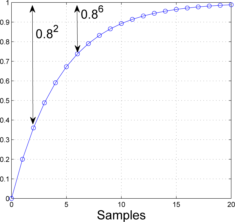
A key concept underlying PFC is that one would like to achieve closed-loop behaviour close to a first order system with a delay td seconds (or m samples), and thus, a key requirement is to identify an input sequence that will achieve this. The target closed-loop behaviour (or reference trajectory) can be expressed as:
where rtr(s) represents the continuous time or Laplace representation and rtr(z) the discrete time or z-transform representation; R is taken to be the actual steady-state target. A typical desired step response, with no delay, is plotted in Figure 1, where, here, the discrete pole is set at ρ = 0.8.
The discrete pole ρ and target time constant Tr are related through the sampling time Ts as
. Some authors prefer to define a target settling time, such as the time it takes to get within 5% of the target (denoted closed-loop time response (CLTR)) and note that Tr ≈ CLTR=3.
2.2. Coincidence Point
The objective is to make the process behave like a pre-specified first order system. This means the desired behaviour is “known”. For example, assuming no delay to simplify the algebra for now and taking yk to be the current output and R to be the steady-state target, one wants the future outputs to follow a first order response from the current value to the target, in other words, to take the following values:
For step targets, PFC chooses a single sample instant in the future, the so-called coincidence horizon ny, and ensures that the actual output prediction matches the target response at that point only. Consequently, the PFC control law reduces to (conceptually), enforcing the equality:
where the notation yk+n|k means the predicted value of y at sample k + n, where the prediction is made at sample k.
Figure 2 illustrates conceptually what is going on. The target trajectory rtr is marked with a dotted line. One forces the output prediction (solid line) to “coincide” at a specified horizon (here, 10 samples into the future). The computation is updated at every sample instant, and this introduces feedback.
Remark 1. The target behaviour Equation (2) and control law requirement Equation (3) can be written down by inspection. Clearly, Equation (2) is simple. Where the system has a delay of “m” samples, the target behaviour should be modified slightly, as discussed in Section 2.4.
Remark 2. One can argue that PFC is intuitive in that one in essence proposes a control move that gets the system output closer (than the current output) to the desired steady state some time in the near future and then continually update this, so in effect, one expects to always be getting closer and closer to the target. However, the main weakness of PFC is the same as its strength. Basing control decision making on a single point will work well if matching that single point implies the rest of the response is also fairly closely matched, as this will imply consistent decision making at each sample. However, conversely, if matching a single point does not imply matching of other parts of the response, then the implied decision making could be seriously flawed, as it could lead to inconsistent decisions from one sample to the next. In simple terms, one needs to be sure that the part of the prediction beyond the coincidence point moves smoothly and monotonically to the steady state.
2.3. Prediction and the PFC Control Law
This section presents PFC for linear discrete models (single input and single output). The decision variable is taken to be the value of the future system input. Moreover, for the purposes of prediction, the system input is assumed to be constant in the future:
so implicitly, within the predictions, one is “expecting” or utilising behaviour close to open-loop dynamics.
2.3.1. First Order Models with Open-Loop Dynamics Equal to Target Dynamics
For a first order model and constant input, prediction is very simple.
For the first order case only, we write the denominator as 1+a1z−1 = 1−az−1, that is a = −a1, as this makes the prediction algebra of Equation (5) easier and more transparent; also, for simplicity, b = b1. Combining this prediction with the coincidence requirement of Equation (3) results in the following equality or essence, the control law.
Theorem 1. If the target pole ρ is chosen equal to the open-loop pole a, that is a = ρ, then the closed-loop pole will match the open-loop pole for any choice of ny (in the nominal case).
Proof. The PFC control Equation (6) is summarised as follows when ρ = a:
where, in effect, K represents the system steady-state gain. As expected, this suggests that input is moved directly to the expected steady-state and is not dependent on the current output. This observation is irrespective of the choice of coincidence horizon ny. Clearly if the input selection is a constant, open-loop dynamics will follow.
2.3.2. First Order Models with Open-Loop Dynamics Different from Target Closed-Loop Dynamics
As the prediction of the output at the coincidence point is based on an assumption of constant input, for large coincidence horizons, it is not intuitively reasonable to request closed-loop behaviours much different from open-loop behaviours, as this will give a significant inconsistency between the assumed input predictions and the actual desired input behaviour to give the required response; in other words, faster responses need over-actuation in transients. Nevertheless, a basic premise of PFC is that one can choose a target pole, so it is worth doing some analysis of the extent to which this really can work effectively. Specifically, we are interested in the extent to which the user selection of ρ is meaningful in that the resulting closed-loop dynamic is close to ρ.
Theorem 2. For first order models, the link between the desired pole ρ and the actual closed-loop pole is weak and is effective only when ny = 1.
Proof. The PFC control and system is summarised as follows when ρ ≠ a:
Eliminating uk, one finds that the closed-loop dynamic is given as:
where γ is a scalar.
The closed-loop pole is therefore defined as:
It is obvious that, as ny increases, the deviation of the pole from a reduces. However, for a coincidence horizon of one, the resulting pole is given as:
Hence, one can achieve the desired pole exactly if ny = 1.
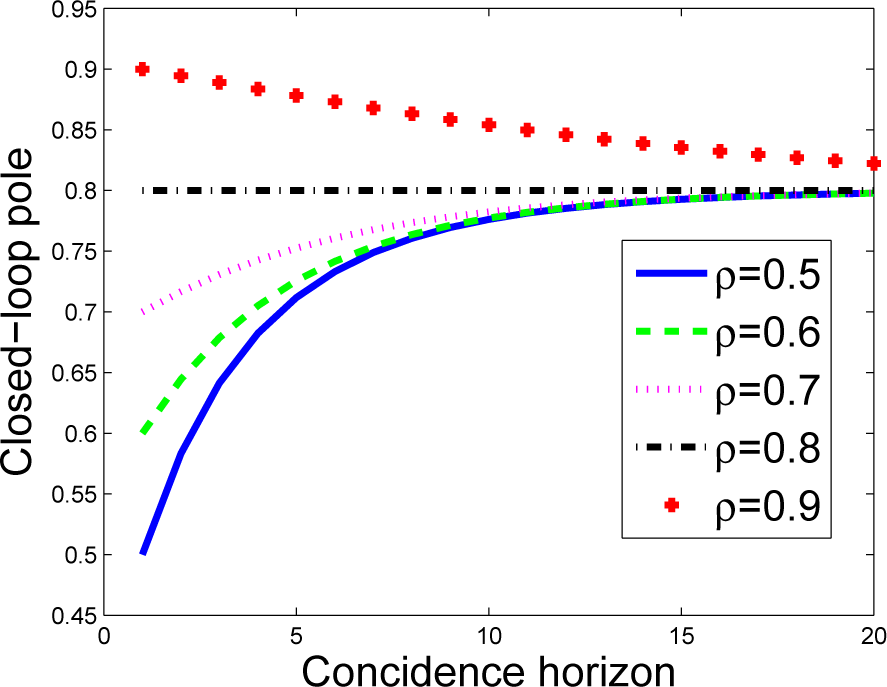
For completeness, Figure 3 shows how the closed-loop pole position varies with the coincidence horizon for various choices of ρ, assuming that a = 0:8; the figure makes it clear that the closed-loop poles tend to a for large ny, but are close to ρ iff ny is small.
Corollary 1. The coincidence horizon and parameter ρ only have a noticeable impact on the control law if the coincidence horizon is small. Irrespective of the choice of ρ, the closed-loop pole tends to a as the coincidence horizon tends to infinity. This is a natural consequence of Equation (10), because:
2.4. First Order Model with Delay
The modification to deal with delays is subtle, but simple, so just a passing comment is given here; with this minor edit, the results of this section all carry across. Clearly, if a system includes a delay, then a reasonable target to follow is a delayed first order response. For a delay of m samples, the target trajectory becomes:
There are two key changes here.
- The replacement of by to take into account the fact that the response cannot begin until after m samples.
- The replacement of process measurement yk by a predicted value yk+m|k; this second change is essential as the target first order response is expected to begin m samples ahead, so the initial error from the target must be based on that sample.
2.5. PFC for Higher Order Models
In the case of higher order models, one cannot easily write down a simple expression for the ny step ahead prediction [8]. It can be shown that for a model of the form (usually, we assume a0 = 1):
then the ny step ahead prediction, with the future inputs fixed, takes the form:
for suitable
,
,
. Consequently, the PFC control law reduces to:
It is immediately clear that in this case, the algebra gives very little insight into the expected control law or closed-loop behaviour and, indeed, the sensitivity to the choice of ny.
Theorem 3. As the coincidence horizon approaches infinity, the PFC control law will reduce to giving open-loop characteristics for a stable open-loop process, irrespective of the choice of ρ.
Proof. For a stable open-loop process, it is easy to show that the prediction parameters of Equation (15) have the following asymptotic properties:
Consequently, the control law becomes:
In other words, the selection of input is the steady-state value required to give no offset and is independent of the current state.
Corollary 2. The PFC code for large coincidence horizons can be reduced to a few trivial lines. This is self-evident from Equation (18).
More general guidance on PFC tuning for higher order models will be discussed in Section 4.
2.6. Model Uncertainty, Offset Free Tracking and Disturbances
It is known that PFC provides robust offset free tracking in the presence of some model uncertainty and disturbances. The detailed algebra is not included in this paper, as it is not a primary focus. Moreover, these details have no impact on the discussions and analysis in this paper, so they are omitted to enable easier reading of the core concepts, although the reader will note that they are included within several of the simulation examples. Therefore, a brief comment only is given here for completeness.
Within PFC, it is common practice to simulate a model (say Gm) in parallel with the process Gp; the model is used for prediction. The difference d = yp−ym between the model output ym and process output yp is taken as an estimate of the system disturbance, although, in fact, it can also correct the offset for parameter uncertainty. The PFC control law that ensures offset free tracking reduces to:
Remark 3. Where a system has real roots only, several PFC practitioners (e.g., [4,9,10]) favour using partial fractions to write the model Gm as a sum of first order models. This has the advantage that the prediction can be written down explicitly in forms like Equation (5) and, thus, with much simpler coding. However, this issue is not central to the current paper.
2.7. Constraint Handling
Constraint handling is a core attribute of PFC; however, the techniques for doing this do not form part of the core or novel contribution of this paper, and thus, the reader is referred to the references for a more detailed discussion [10]. It should be noted of course that that the proposals given in this paper fit within a conventional PFC approach, and thus, standard PFC constraint handling procedures can be deployed.
2.8. Summary of PFC Tuning
It is clear that for first order systems, the PFC approach will work well as a means of designing a control law that will give dynamics close to the open-loop behaviour and offset free tracking. Moreover, one can use PFC as an effective way of changing the dynamics, as long as the coincidence horizon is small, preferably one. Section 3 will give some numerical examples to reinforce this.
For systems with more complex dynamics, it is less transparent whether PFC will work well or not. Given the complexity of Equation (16), existing analysis does not give any useful generic results beyond Theorem 3. Consequently, there is a need for some better insight into when PFC is appropriate and how it might be tuned. Section 4 will present some proposals along with numerical illustrations.
3. Numerical Illustrations for First Order Systems
This section will look at the tuning of PFC through a number of first order examples and demonstrate the impact of changing the parameters ρ; ny.
3.1. Concepts of Well-Posed Decision Making
Within predictive control, the concept of well-posed decision making is based on the consistency in subsequent samples of any decisions made. In other words, if one determines a strategy now that is supposedly good for the long term, then one would expect that at the next sample, the updated strategy would be very similar. Substantial changes in strategy from one sample to the next are an indicator of inconsistency, which could lead to chaos and most certainly are not a solid foundation for a control law.
In this section, the figures presented will give two line plots:
- The implied PFC prediction at a given sample (denoted up; yp for the input and output, respectively).
- The actual closed-loop behaviour that results (denoted us; ys for the input and output, respectively).
The indicator we are looking at for well-posed decision making is that prediction and behaviour are similar, and most certainly, the change from one sample to the next should be small.
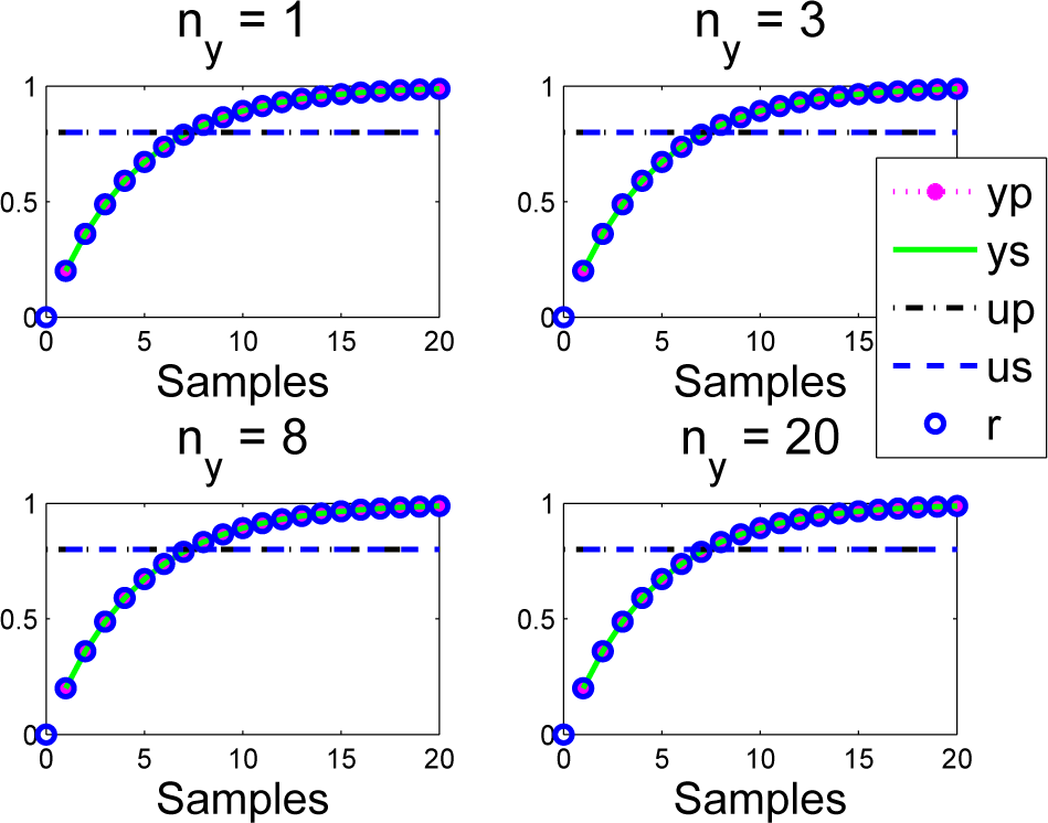
3.2. PFC Responses with Target Behaviour Equal to Open-Loop Behaviour
Take a first order model (1−az+1)yk = bz−1uk; without loss of generality, we will use a = 0:8; b = 0:25 for the simulation, as the observations here are based around selecting ρ = a. Plot the closed-loop responses for various choices of coincidence horizon and overlay the predictions made at the first sample. The results are given in Figure 4. What is immediately clear is that the predictions and closed-loop behaviour overlap (ys = yp) precisely (as expected from Theorem 1) in the nominal case, so in this case, PFC gives well-posed decision making.
For completeness, a Figure 5 shows responses for an equivalent system with a delay; the same observations follow as expected.
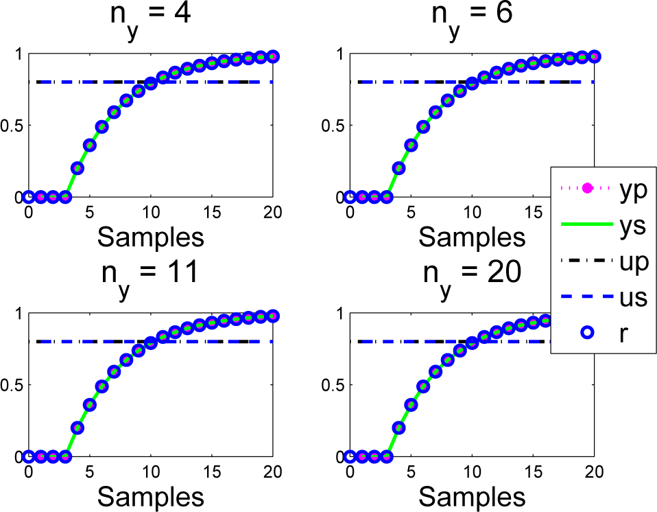
3.3. PFC Responses with Target Behaviour Different from Open-Loop Behaviour
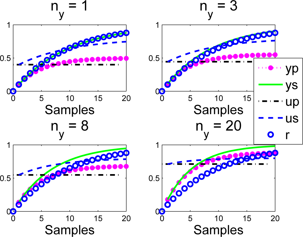
Take the same model as in the previous section, but use time constants a little faster ρ < a (Figure 6) and a little slower ρ > a (Figure 7) than the open-loop dynamics. Again, investigate various choices of the coincidence horizon. The actual closed-loop dynamic behaviour is strongly linked to the choice of ny, as discussed in Section 2.3.2, but here, we are also interested in the consistency of the decision making, so the figures overlay the implied predictions utilised by PFC and, of course, the target dynamic.
- When ρ ≠ a, for small ny, there is clearly some inconsistency from one sample to the next, as the input prediction up at the first sample is different from the closed-loop evolution us that results. For example, when ρ = 0:7; a = 0:8; ny = 1, the input change from Sample 1 to Sample 2 is from 1.2 to 1.08.
- Despite the inconsistency between implied predictions yp and actual behaviour ys, with ny = 1, the target behaviour r has been achieved.
- As ny increases, the choice of ρ becomes less and less significant (the output yp does not track the target r), but there is much better consistency between predictions yp and behaviour ys.
Remark 4. There is an interesting inconsistency noted here. If the coincidence horizon is small, the design parameter ρ is effective in changing the closed-loop dynamics, but the implied long-term predictions are a poor indicator of final behaviour. Conversely, if the coincidence horizon is large, the design parameter ρ has no affect, but the predictions are consistent. Of course, readers may note that PFC never claimed to take any account of long-term predictions within the decision making process, and therefore, it was not implicit that one would keep the input constant at future samples!
4. Tuning PFC for Higher Order Systems
The reader will not be surprised with the observation that PFC may be less effective when the expectation of a closed-loop behaviour close to a first order response is invalid or not realistic, as with higher order systems, and therefore, more care is needed. A weakness of PFC is the lack of the explicit inclusion of long-term effects. While for systems with simple first order dynamics this matters little, the repercussions for systems with more challenging dynamics can be more serious, especially if one introduces constraint handling (some examples are in Section 5). Although a well-trained PFC user can demonstrate that PFC works well if tuned effectively, it is important to understand the difficulties that can arise if one makes poor tuning decisions.
In cases where the open-loop response does not include significant oscillation or instability and moves smoothly to the steady state, it is possible to demonstrate that matching the step response to a first order response at some point in the future still makes good intuitive sense and is likely to lead to a well-posed decision making or control law; of course, this is notwithstanding the fact that a rigorous proof or analysis is future work and may even not be possible in many cases. This section will give some demonstrations of how one can be systematic at designing a PFC control law that works reasonably well, that is choosing a coincidence horizon that works reasonably well and achieves close to the target time constants.
4.1. Coincidence Horizon Issues with Higher Order Models
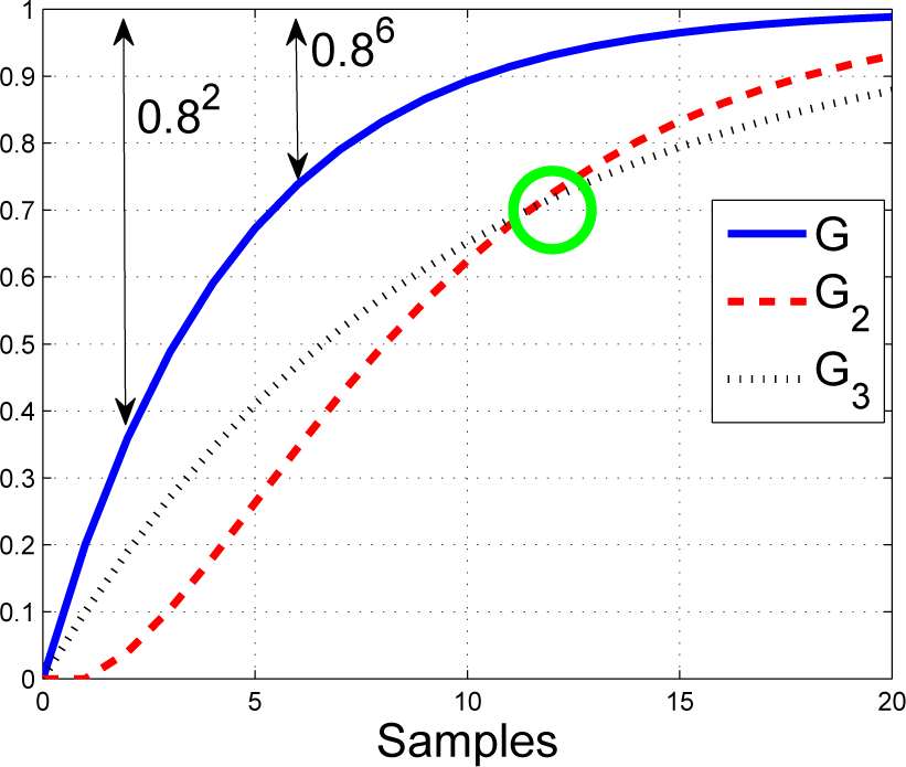
It is normal for higher order systems, even over-damped ones, to have a lag in their step response, and consequently, forcing the system output to precisely match a typical first order response could be counter intuitive. See Figure 8 for an example of this; the figure overlays the step responses of:
From this observation, it is rather obvious that using a coincidence horizon of one for higher order systems makes no sense at all, and indeed, one may need to target a much slower implied first order pole, such as G3, along with a higher coincidence horizon (ny = 12 is marked in this figure) to get sensible answers! Indeed, it can be shown that using ny = 1 can imply a controller using “plant inversion”, which is not robust.
Readers will note that one can only force coincidence with faster poles (G2 and G) by having over actuation during transients, so the implied steady state within the prediction is well above the target. Readers are also reminded, however, of Theorem 3 and that using too large ny PFC essentially reduces to choosing the steady-state input, so the tuning parameter ρ would have a smaller affect.
The proposal here is linked to the underlying common sense or intuitive nature of the PFC approach, that is the argument that the part of the prediction which is ignored (further into the future than the coincidence point) is implicitly moving closer to the desired steady-state, and hence, iterative decision making will be well posed if it gradually moves the coincidence point nearer and nearer to the target (in absolute terms). This will happen automatically if ny is based on a point where the step response is increasing, and changes relative to the steady state are close to monotonic thereafter.
Conjecture 1. For systems with close to monotonically convergent behaviour after immediate transients, a good choice of coincidence horizon is one where the open-loop step response has risen to around 40% to 80% of the steady state and the gradient is significant (formal proofs and details constitute future work).
Remark 5. A manual for training engineers [4,5] on PFC suggests that a suitable value for ny might also be determined by identifying the so-called inflexion point on the step response curve, that is, where the gradient is maximum. However, care must be exercised, as the maximum gradient may not be enough on its own, especially with non-minimum phase systems, as noted briefly with system G4.
4.2. PFC Tuning for Systems with Relatively Simple Dynamics
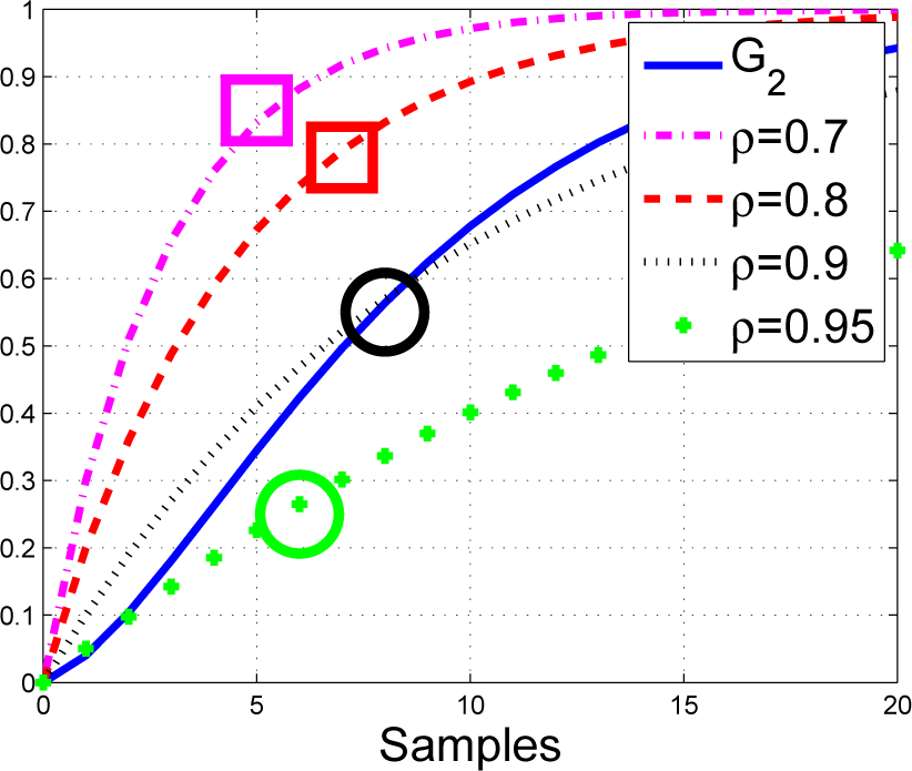
Consider a simple second order system:
and overlay the trajectories of several typical targets with the actual open-loop step response (see Figure 9) and possible choices of coincidence points.
- Following Conjecture 1 and due to the lag in the process (the step response takes a few samples to start moving significantly), it is not reasonable to use ny < 5. Similarly, ny > 15 will put too much emphasis on the steady state.
- It is clear that for ρ = 0:9, an intercept exists between the step response and target, and hence, ny = 8 would be a logical choice of coincidence point.
- For smaller and larger choices of ρ, there is no intercept in the range 5 ≤ ny ≤ 15, and hence, to force coincidence (essentially to move the step response up or down), PFC will either have to under- or over-actuate using these choices of ρ. This is what we expect, as a faster ρ requires over-actuation and a slower ρ requires under-actuation.
- Limits on the actuation permitted will be a guide as to what range of ρ is permissible to request and, indeed, the appropriate ny. For example, ρ = 0:7 requires an input over actuation of around 2.5 to get coincidence at ny = 5 or around 1.8 if ny = 8.
The actual closed-loop responses with PFC are given in Figure 10, and these reinforce the comments above: faster ρ (that is smaller values of ρ) requires over-actuation in transients, a choice of ρ = 0:8 and exact coincidence, giving an almost constant input and a slower ρ (that is, ρ > 0:8), giving under-actuation. In all cases, it is clear that a sensible choice of ny has resulted in the choice of ρ being an effective tuning parameter, that is the closed-loop outputs converge roughly at the same speed as the target.
4.3. PFC Tuning for a Non-Minimum Phase System
Next, take a third order system with some non-minimum phase characteristics, but otherwise smooth behaviour.
Overlay the responses of several typical targets with the actual open-loop step response (see Figure 11). Due to non-minimum phase characteristic, it is clear that using Conjecture 1, the coincidence horizon should be in the range 7 ≤ ny ≤ 12. Potential choices of coincidence points are marked on the figure. Readers may also note that the inflexion point is around ny = 5, and clearly, as the magnitude of the step response is still very small here, such a design choice for ny is inappropriate and can be shown to give very poor closed-loop performance!
The actual closed-loop responses with PFC are given in Figure 12, and these reinforce the expectations. Notwithstanding the fact that one cannot follow a first order target in immediate transients due to the non-minimum phase characteristic, nevertheless, as long as ny is well chosen, the choice of ρ has been effective in affecting the closed-loop settling time and input activity, and thus, ρ is an effective tuning parameter.
4.4. PFC Tuning for an under-Damped System
Next, take an under-damped system.
Overlay the responses of several typical targets with the actual open-loop step response (see Figure 13). In order to follow Conjecture 1, it is better to select a coincidence horizon in the range 3 ≤ ny ≤ 6. Potential choices of the coincidence point are marked on the figure.
The actual closed-loop responses with PFC are given in Figure 14, and once again, it is seen that the choice of ρ has been effective in affecting the closed-loop settling time and input activity and, thus, is an effective tuning parameter.
4.5. Summary
This section has shown that even for processes with underlying dynamics that are not close to a first order system, nevertheless, PFC can be an effective strategy and, moreover, the tuning parameter ρ, that is the target closed-loop time constant, can be used effectively. This, of course, is invaluable to technical users who wish to specify response times rather the controller gains. In practice, the desired settling time (CLTR) is used, which can be represented as an equivalent ρ, as shown earlier. It is noted that one needs to select the coincidence horizon carefully, and the proposal here involves an overlaying of typical targets with the open-loop step response as a simple mechanism (Conjecture 1) of identifying a suitable ny. One can, of course, do an iterative design, underpinned by simulations with various ny, to determine the final choice.
5. PFC for Processes with Difficult Dynamics
It was hinted in earlier sections that the main concepts in PFC may not carry over well to processes with oscillatory, unstable or other non-simple dynamics. In simple terms, the assumption of a constant input is not sufficient to create an output that will have good characteristics [11]. In order then to make PFC more effective and easier to tune, it may be necessary to undertake some pre-conditioning to form input predictions and possibly output targets, which are more realistic, but notably, without following the normal predictive control route of performance indices and quadratic programming optimisations, which are non-trivial to implement. This section illustrates some of those scenarios, and notably, these are systems that fail the core requirements to apply Conjecture 1.
5.1. Second Order Model with Oscillatory Dynamics
It is clear that a system with oscillatory dynamics cannot easily match a first order target. Moreover, it is intuitively obvious that matching the predicted response at a single coincidence point in the future could be a very poor indicator of actual closed-loop behaviour. The tuning difficulties are well illustrated with the following system:
The results of using PFC are given in Figure 15 and in essence demonstrate:
- PFC gives good results with ρ = 0:7; ny = 2; 3 (fails totally for ny = 1), but it is difficult to argue that this is more than just a fluke, given that the shapes of the closed-loop input trajectory are not close to a constant.
- For large horizons, the open-loop dynamic dominates and the behaviour is unacceptable.
5.2. Model with Open-Loop Unstable Dynamics
There has been some brief discussion of using PFC with open-loop unstable processes in the past [12]; the proposal there was to prestabilise the predictions by cancelling unstable modes [11] before applying a PFC algorithm. However, before we return to discussions on how the base PFC algorithm could be modified (future work), it is worth demonstrating the extent to which it is effective in its base form. The tuning difficulties are well illustrated with the following system and ρ = 0:8:
The results of using PFC are given in Figure 16 and, in essence, demonstrate the following:
- PFC fails for both ny = 1 and large ny.
- In this case, reasonable behaviour results for ny = 3, but it would be difficult to argue that this is a systematic design; and certainly, the parameter ρ has not been effective.
5.3. Summary
For many systems, the tuning of PFC is not obvious, and the designer is left with, in effect, a global search across ρ; ny, but without a clear expectation of whether this will give a good result or not. Intuitively, the core failing is the desire to follow a first order trajectory, and using a constant future input as this is clearly unrealistic for systems with complex dynamics. Therefore, to extend the benefits of PFC, one needs to extend the target behaviours and/or input parametrisations. It should be emphasised, however, that PFC practitioners have work-arounds, and modifications for these scenarios and future work will investigate those proposals in depth, alongside the consideration of alternative modifications.
- A reasonable conjecture is that one should begin from a target trajectory that is realistic, as then, ensuring the predictions are close to this trajectory would give a high expectation of good behaviour.
- For systems with oscillatory open-loop dynamics, it is reasonable to conjecture that the future control input should be shaped so that the impact of this oscillation is minimised.
- For unstable open-loop processes, it is well known that one should parametrise the future decisions in such a way that the predictions are all guaranteed convergent [7], preferably to the correct steady state.
In summary, therefore, rather than using the next value of the input uk as the control decision and assuming that all future inputs are constant, one needs alternative parametrisations, which ensure that the process has underlying good behaviour and, within that parametrisation, include some flexibility that can be used to influence the speed of response.
6. Conclusions
This paper has provided an elementary analysis of PFC and the expected behaviour and tuning. It is clear that generic stability and performance results may not be possible, in general, and, here, have been determined rigorously only for the simple first order case.
6.1. Key Points
For the first order case, it was shown that the choice of pole is meaningful only for a coincidence horizon of one. As the coincidence horizon is increased, this parameter has a decreasing effect on the control law and resulting closed-loop behaviour, and indeed, for high ny, the PFC control law reduces to estimating the process steady state input; thus, ρ has no impact at all.
For higher order systems, the tuning rules and efficacy of the parameters ρ, ny are not consistent and vary from one example to another depending on the underlying process dynamics. Consequently, some suggestions were made as to how one could determine an appropriate range of ny, ρ before any fine tuning. The methodology was demonstrated on several examples and found to be effective and, moreover, is similar, but not identical, to the empirical suggestions in [4].
Finally, a rather simple, but useful observation, is that PFC with a large coincidence horizon reduces to an integral control law, which gives a closed-loop with open-loop dynamics (or so-called mean-level control, as noted elsewhere in the predictive control literature). Where such behaviour is acceptable, one can vastly simplify the current PFC code to just a few lines, and moreover, in cases of only input constraints, even the constraint handling becomes trivial.
6.2. Future Work
Aside from the need to consider whether one can give more rigorous tuning rules with guarantees of behaviour or performance with higher order systems, there are also a number of issues not covered here that would be interesting and should be pursued next. For example, one advantage of PFC is the ease with which one can target ramps and parabolas with no offset or lag, so it would be interesting to develop some analysis of how that can be done systematically. When does it work well and what sorts of scenarios produce challenges? Are there simple improvements that can be suggested?
In a similar vein, the constraint handling approaches of PFC are relatively simple, and thus, it is easy to find examples where the strategies would fail. However, the more important point is that for many realistic scenarios, it works quite well, and with a very simple approach to code and maintain. Hence, once again, it would be useful to provide a more formal analysis of the efficacy of PFC approaches to constraint handling.
Finally, it was noted that there do not exist simple proposals in the literature for how the simple concepts of PFC can be adapted to deal with some challenging dynamics; this would be worthwhile, as the benefits of easy coding and tuning would make such proposals useful.
Acknowledgments
Thanks to Jacques Richalet, the founder of PFC, for many discussions and supporting code.
Author Contributions
This paper is a collaborative work between both authors. R.H. focussed on the accurate communication of the concepts and J.A.R. provided initial proposals and coding.
Conflicts of Interest
The authors declare no conflict of interest.
References
- Rossiter, J.A.T. Model-Based Predictive Control: A Practical Approach; CRC Press: London, UK, 2003. [Google Scholar]
- Maciejowski, J. Predictive Control with Constraints; Prentice Hall: Harlow, UK, 2001. [Google Scholar]
- Richalet, J.; Rault, A.; Testud, J.L.; Papon, J. Model predictive heuristic control: Applications to industrial processes. Automatica 1978, 14, 413–428. [Google Scholar]
- Richalet, J.; O’Donovan, D. Predictive Functional Control: Principles and Industrial Applications; Springer-Verlag: London, UK, 2009. [Google Scholar]
- Richalet, J.; Lavielle, G.; Mallet, J. Commande Predictive; Eyrolles: Paris, France, 2004. [Google Scholar]
- Scokaert, P.O.M.; Rawlings, J.B. Constrained linear quadratic regulation. IEEE Trans. Autom. Control 1998, 43, 1163–1168. [Google Scholar]
- Rossiter, J.A.; Rice, M.J.; Kouvaritakis, B. A numerically robust state-space approach to stable predictive control strategies. Automatica 1998, 34, 65–73. [Google Scholar]
- Rossiter, J.A. Notes on multi-step ahead prediction based on the principle of concatenation. Proc. Inst. Mech. Eng. I J. Syst. Control Eng. 1993, 207, 261–263. [Google Scholar]
- Khadir, M.T.; Ringwood, J.V. Extension of first order predictive functional controllers to handle higher order internal models. Int. J. Appl. Math. Comput. Sci. 2008, 18, 229–239. [Google Scholar]
- Haber, R.; Bars, R.; Schmitz, U. Predictive Control in Process Engineering: From the Basics to the Applications, Chapter 11: Predictive Functional Control; Wiley-VCH: Weinheim, Germany, 2011. [Google Scholar]
- Rawlings, J.B.; Muske, K.R. The stability of constrained receding horizon control. Trans. IEEE Autom. Control 1993, 38, 1512–1516. [Google Scholar]
- Rossiter, J.A.; Richalet, J. Handling constraints with predictive functional control of unstable processes. Am. Control Conf. 2002, 6, 4746–4751. [Google Scholar]
Figure 1.
Target closed-loop step response with a pole of 0.8 and no delay.

Figure 2.
Conceptual illustration of PFC control law definition matching prediction to target trajectory at a single point.
Figure 2.
Conceptual illustration of PFC control law definition matching prediction to target trajectory at a single point.
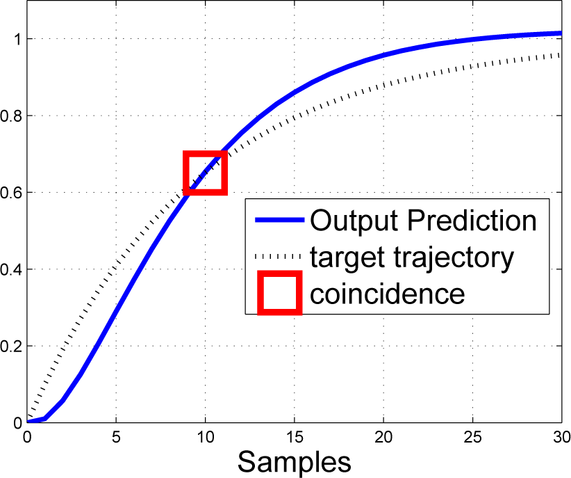
Figure 3.
Closed-loop pole dependence upon coincidence horizon and ρ for a = 0:8.

Figure 4.
Closed-loop PFC input and output us; ys responses overlaid with predictions up; yp made at the first sample for a = ρ; here, ys = yp; us = up.
Figure 4.
Closed-loop PFC input and output us; ys responses overlaid with predictions up; yp made at the first sample for a = ρ; here, ys = yp; us = up.

Figure 5.
Closed-loop PFC input and output us; ys responses overlaid with predictions up; yp made at the first sample for a = ρ; here, ys = yp; us = up for system with a three-sample delay.
Figure 5.
Closed-loop PFC input and output us; ys responses overlaid with predictions up; yp made at the first sample for a = ρ; here, ys = yp; us = up for system with a three-sample delay.

Figure 6.
Closed-loop PFC input and output us; ys responses overlaid with predictions up; yp made at the first sample for a > ρ.
Figure 6.
Closed-loop PFC input and output us; ys responses overlaid with predictions up; yp made at the first sample for a > ρ.
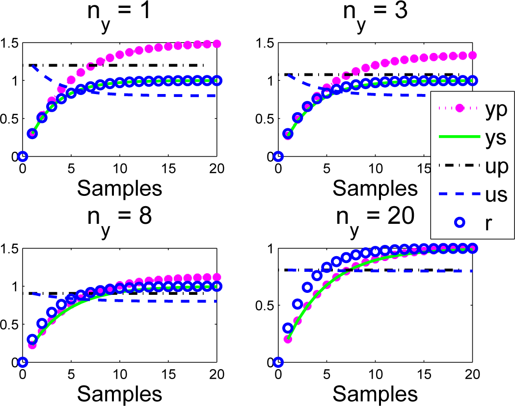
Figure 7.
Closed-loop PFC input and output us; ys responses overlaid with predictions up; yp made at the first sample for a < ρ.
Figure 7.
Closed-loop PFC input and output us; ys responses overlaid with predictions up; yp made at the first sample for a < ρ.

Figure 8.
Target first order step response with poles of 0.8 and 0.9 overlaid with a step response of a second order system.
Figure 8.
Target first order step response with poles of 0.8 and 0.9 overlaid with a step response of a second order system.

Figure 9.
Open-loop step response overlaid with several possible targets and potential coincidence points.
Figure 9.
Open-loop step response overlaid with several possible targets and potential coincidence points.

Figure 10.
Closed-loop step responses for a second order system G2 with various ρ; ny overlaid with the underlying target trajectory.
Figure 10.
Closed-loop step responses for a second order system G2 with various ρ; ny overlaid with the underlying target trajectory.

Figure 11.
Open-loop step response of G4 overlaid with several possible targets and potential coincidence points for a non-minimum phase system.
Figure 11.
Open-loop step response of G4 overlaid with several possible targets and potential coincidence points for a non-minimum phase system.
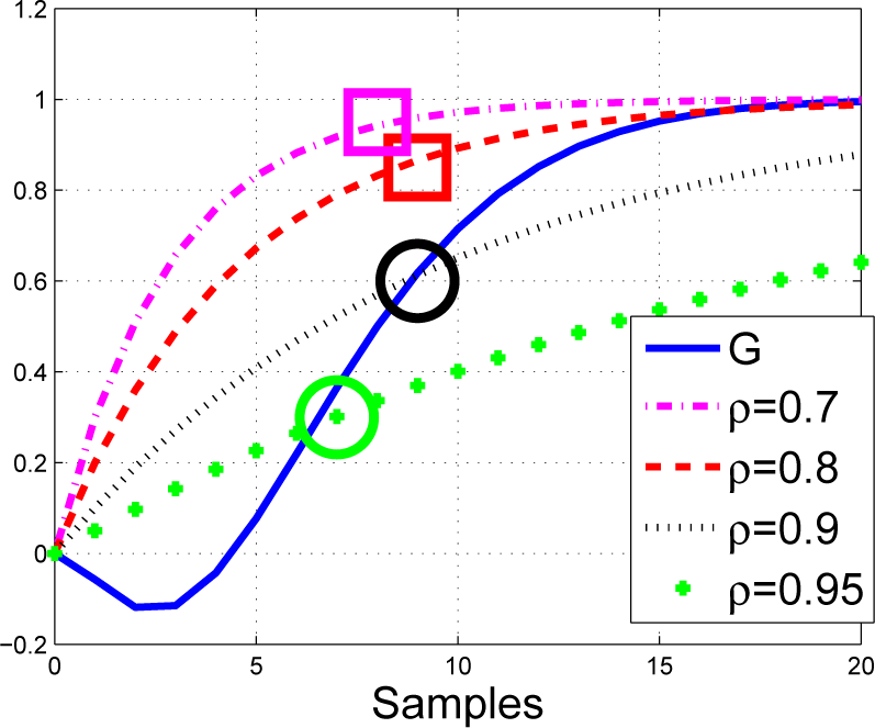
Figure 12.
Closed-loop step responses for a third order system G4 with various ρ; ny overlaid with the underlying target trajectory.
Figure 12.
Closed-loop step responses for a third order system G4 with various ρ; ny overlaid with the underlying target trajectory.
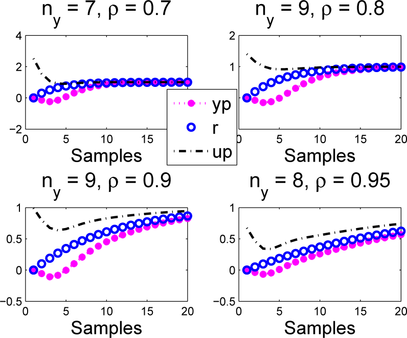
Figure 13.
Open-loop step response of G5 overlaid with several possible targets and potential coincidence points for an under-damped system.
Figure 13.
Open-loop step response of G5 overlaid with several possible targets and potential coincidence points for an under-damped system.

Figure 14.
Closed-loop step responses for an under-damped system G5 with various ρ; ny overlaid with the underlying target trajectory.
Figure 14.
Closed-loop step responses for an under-damped system G5 with various ρ; ny overlaid with the underlying target trajectory.
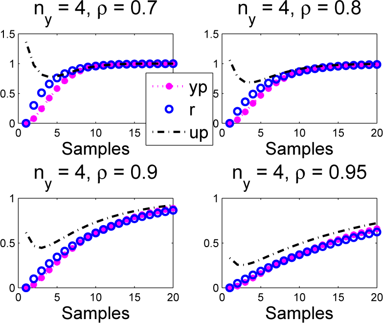
Figure 15.
Closed-loop PFC input and output us; ys responses overlaid with predictions up; yp made at the first sample for an oscillatory system G6.
Figure 15.
Closed-loop PFC input and output us; ys responses overlaid with predictions up; yp made at the first sample for an oscillatory system G6.
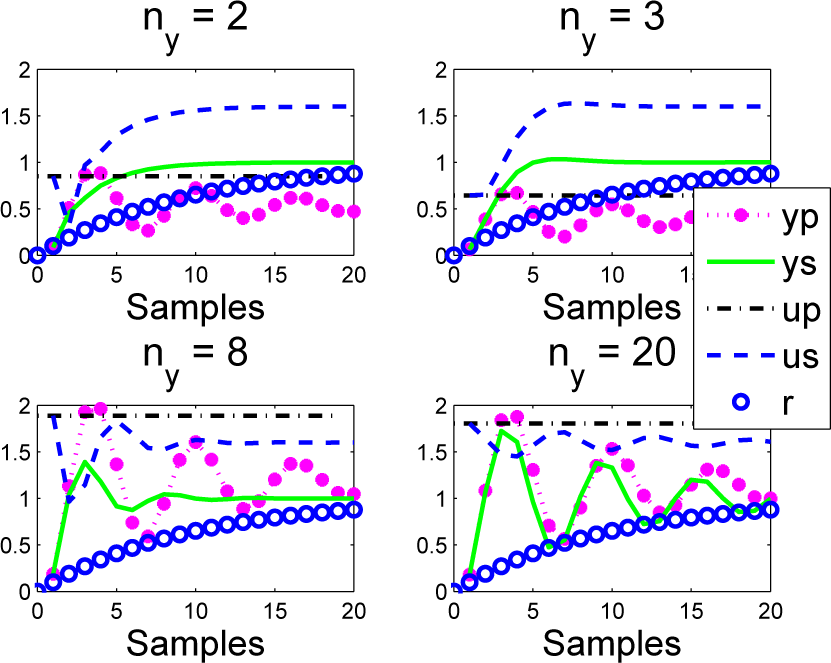
Figure 16.
Closed-loop PFC input and output us; ys responses overlaid with predictions up; yp made at the first sample for unstable process G7.
Figure 16.
Closed-loop PFC input and output us; ys responses overlaid with predictions up; yp made at the first sample for unstable process G7.

© 2015 by the authors; licensee MDPI, Basel, Switzerland This article is an open access article distributed under the terms and conditions of the Creative Commons Attribution license (http://creativecommons.org/licenses/by/4.0/).
Share and Cite
MDPI and ACS Style
Rossiter, J.A.; Haber, R. The Effect of Coincidence Horizon on Predictive Functional Control. Processes 2015, 3, 25-45. https://doi.org/10.3390/pr3010025
AMA Style
Rossiter JA, Haber R. The Effect of Coincidence Horizon on Predictive Functional Control. Processes. 2015; 3(1):25-45. https://doi.org/10.3390/pr3010025
Chicago/Turabian StyleRossiter, John Anthony, and Robert Haber. 2015. "The Effect of Coincidence Horizon on Predictive Functional Control" Processes 3, no. 1: 25-45. https://doi.org/10.3390/pr3010025