
Alt-Splice Gene Predictor Using Multitrack-Clique Analysis: Verification of Statistical Support for Modelling in Genomes of Multicellular Eukaryotes

Abstract
:1. Introduction
2. Background
2.1. The Standard 1st Order HMM
- A hidden state alphabet, Λ, with “Prior” Probabilities P(λ) for all λ Λ, and “Transition” Probabilities P(λ2|λ1) for all λ1 λ2 Λ—where the standard transition probability is denoted akl = P(λn = l|λn−1 = k) for a 1st order Markov model on states with homogenous stationary statistics (i.e., no dependence on position ‘n’).
- An observable alphabet, B, with “Emission” Probabilities P(b|λ) for all λ Λ b B—where the standard emission probability is ek(b) = P(bn = b|λn = k), i.e., a 0th order Markov model on bases with homogenous stationary statistics.
- Evaluation—Determine the probability of occurrence of the observed sequence.
- Learning (Baum–Welch)—Determine the most likely emission and transition probabilities for a given set of observational data.
- Decoding (Viterbi)—Determine the most probable sequence of states emitting the observed sequence.
2.2. The Meta-State HMM
- 1)
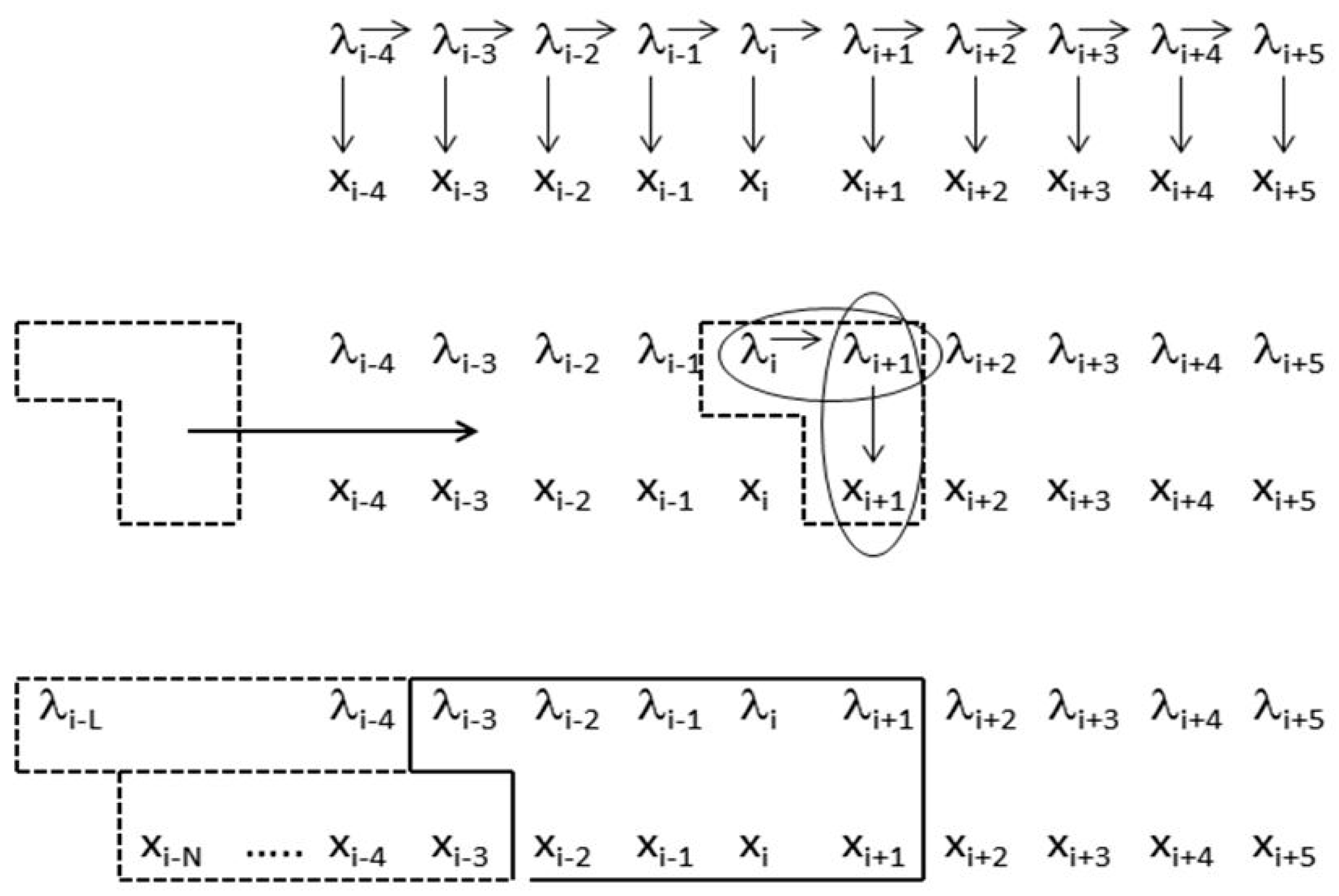
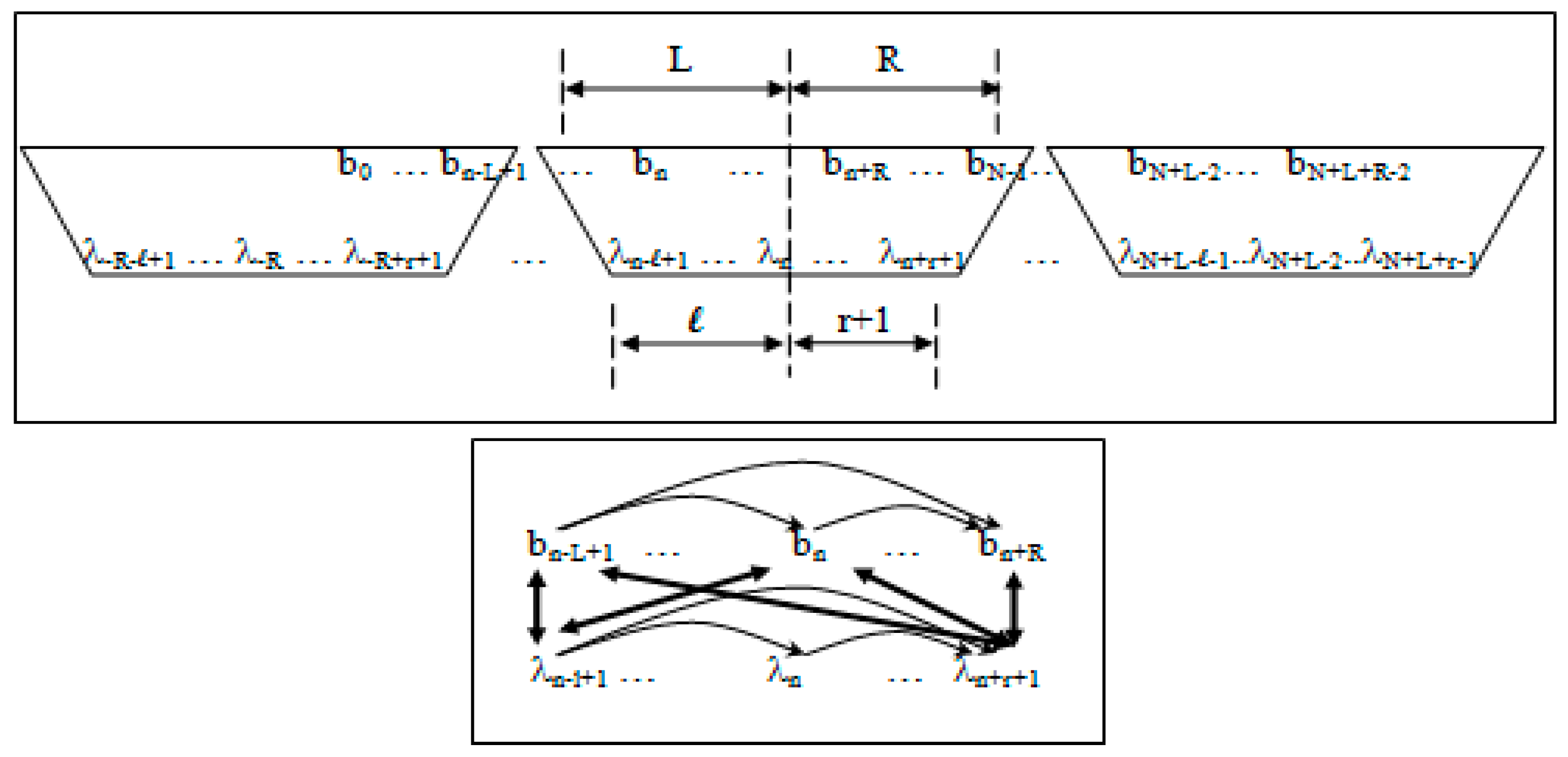
- Non-negative integers L and R denoting left and right maximum extents of a substring, wn, (with suitable truncation at the data boundaries, b0 and bN−1) are associated with the primitive observation, bn , in the following way:
- wn = bn−L+1, …, bn, …, bn+R
- n = bn−L+1, …, bn, …, bn+R−1
- 2)
- Non-negative integers l and r are used to denote the left and right extents of the extended (footprint) states, f. Here, we show the relationships among the primitive states λ, dimer states s, and footprint states f:
- δn = λnλn+1 (dimer state, length in λ’s = 2)
- fn = δn−l+1, …, δn+r ≅ λn−l+1, …, λn, …, λn+r+1 (footprint state, length in δ’s = l + r)
2.3. HMM States and Transitions for Gene-Structure Identification
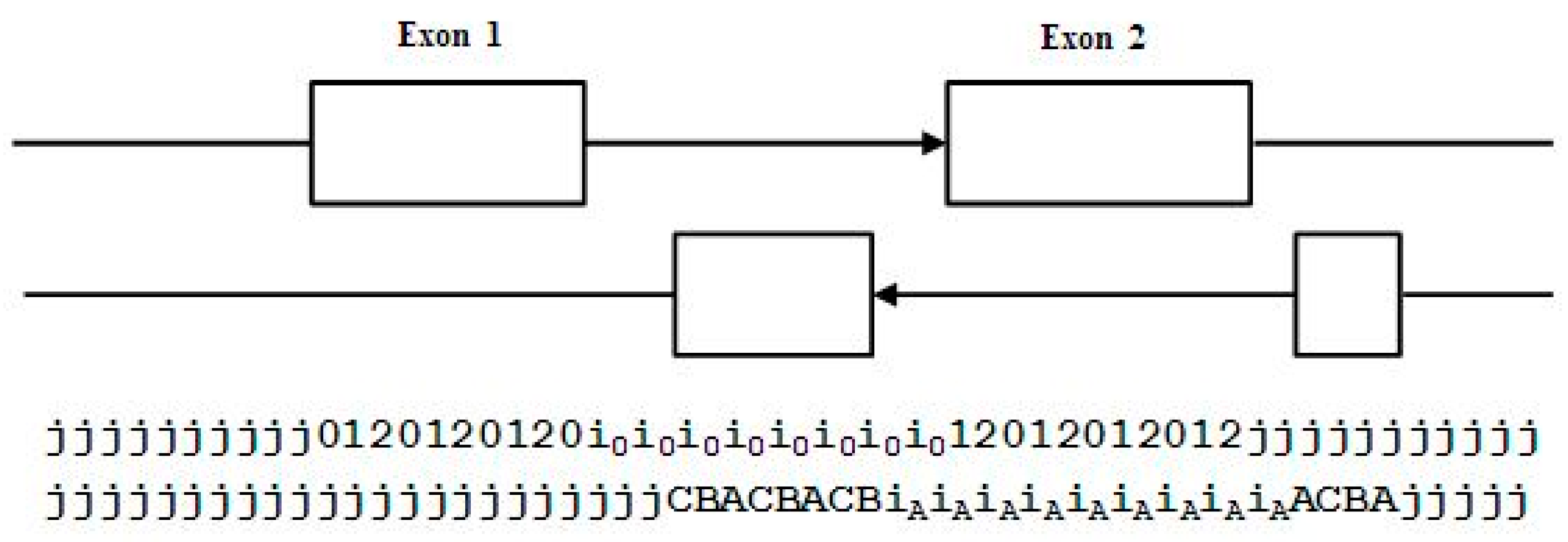
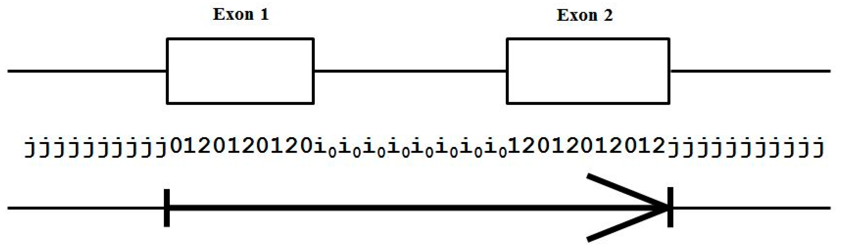
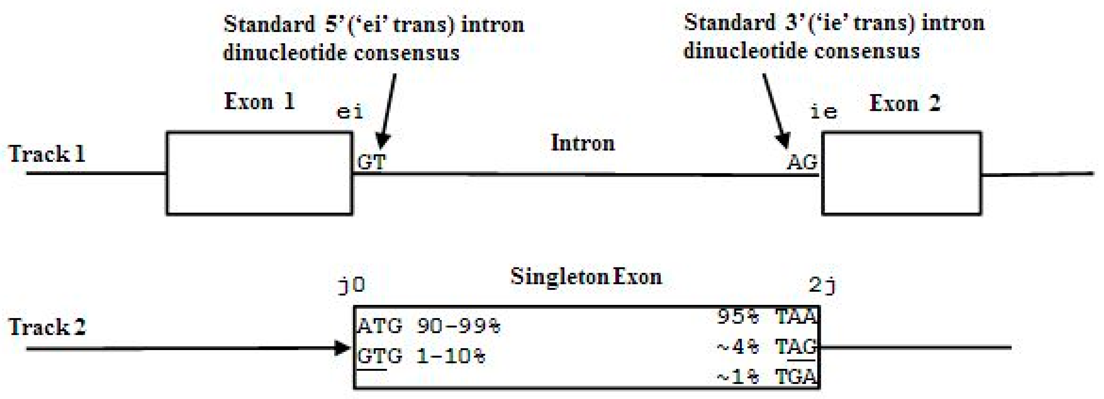
- Exon states = {e0, e1, e2}, where frame label is ‘real’, i.e., there are three emission tables;
- Intron states = {i0, i1, i2}, where frame label is a convenient implementation artifact (so one em table);
- Junk state = {j}, the non-coding (non-exonic) nucleotides in the intergenic regions, while the non-coding nucleotides in the intragenic regions are the aforementioned introns.
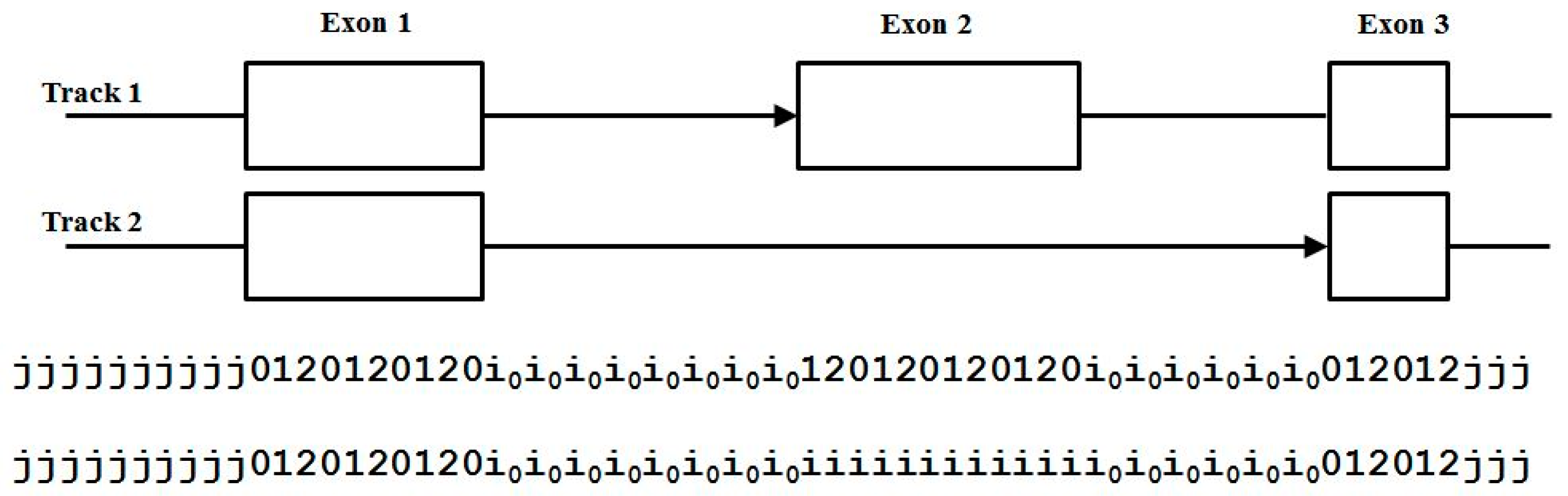
- jj...je0e1e2…e0i0i0…i0e1…e0e1e2jj…j (intron follows exon base with frame 0)
- jj...je0e1e2…e1i1i1…i1e2…e0e1e2jj…j (intron follows exon base with frame 1)
- jj...je0e1e2…e2i2i2…i2e0…e0e1e2jj…j (intron follows exon base with frame 2)
3. Experimental Section—Methods
3.1. Genome Versions Used in Data Analysis (All from www.ensembl.org)
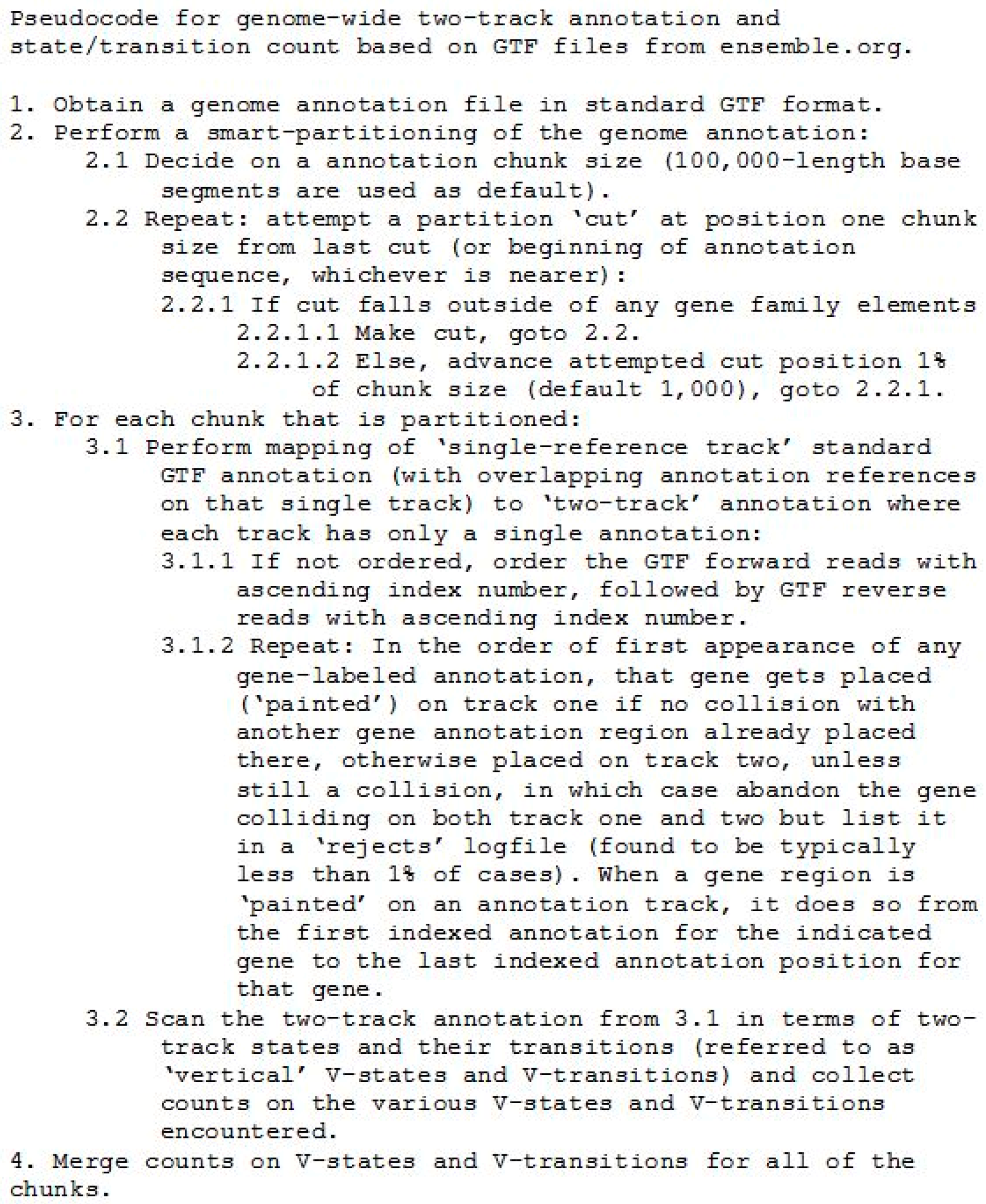
3.2. Pre-Partitioning Training Data for Massively Parallel/Distributed Solutions
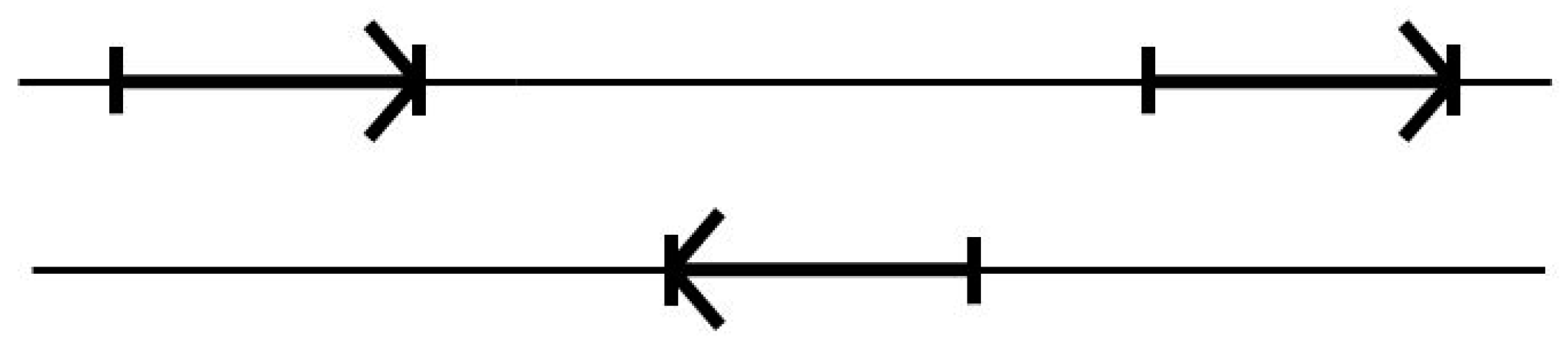
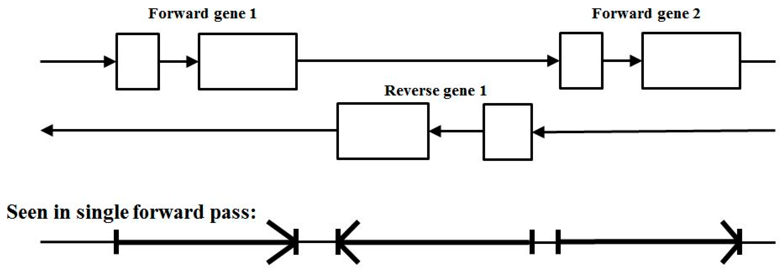
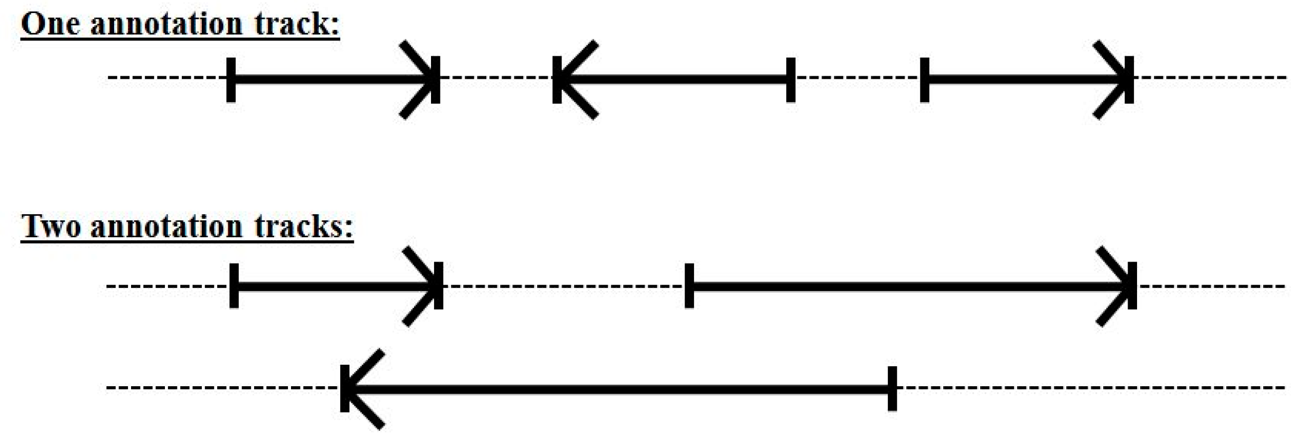
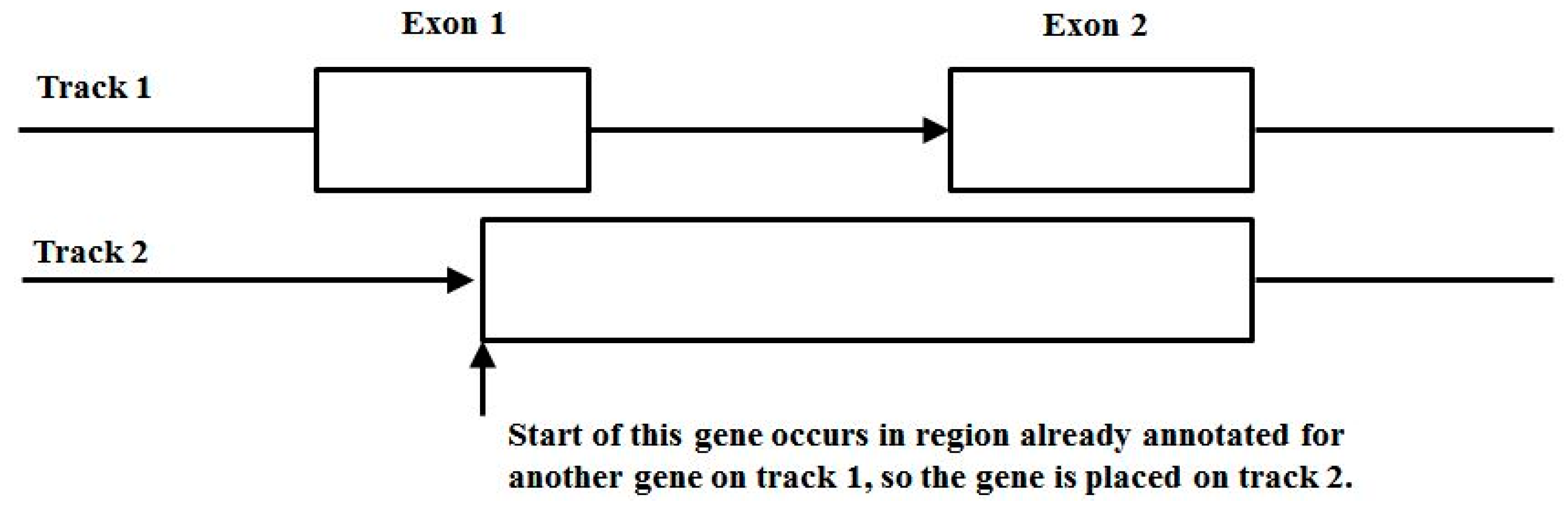
3.3. Two-Track Annotation and Counting—Order of Annotation Governs Track Placement
4. Results
- (3′|i) V-transitions: i0ii, i1ii, i2ii, iii0, iii1, iii2, AIII, BIII, CIII, IIAI, IIBI, IICI.
- (5′|i) V-transitions: 0iii, 1iii, 2iii, ii0i, ii1i, ii2i, IAII, IBII, ICII, IIIA, IIIB, IIIC.
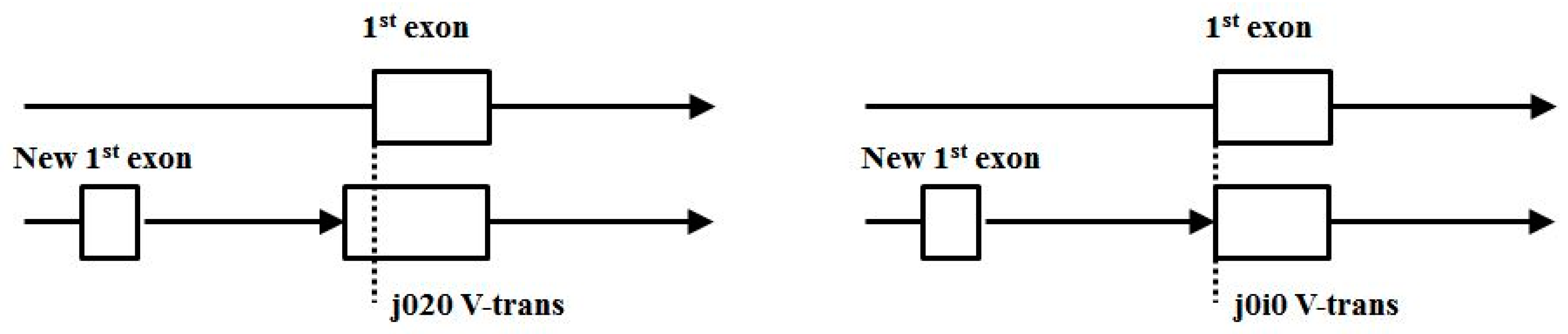
- (3′|e) V-transitions: 01i1, 12i2, 20i0, i020, i101, i202, AIAC, BIBA, CICB, BABI, CBCI, ACAI.
- (5′|e) V-transitions: 0i01, 1i12, 2i20, 010i, 121i, 202i, IABA, IBCB, ICAC, BAIA, CBIB, ACIC.
5. Discussion
5.1. V–Transition Rules
- (1)
- Approximate frame agreement rule: j0 on track 1 cannot overlap 2j, 0i, 1i, i1, i2 on track 2, and only rarely overlap with 01 or 12 on track 2 (a consensus agreement rule). {j0, jC, 2j, Aj} similar, so excluding 4 × 5 = 20. Similarly with 01 track 1 not overlapping with 12, 20, 1i, 2i, i0, i2 on track 2 (rarely with j0 and 2j as noted). {10.12.20.BA, CB, AC} similar, so excluding 6 × 6 = 36 V–transitions. Similarly 0i on track 1 cannot overlap with j0, 2j, 12, 20, 1i, 2i, i0, i2 on track 2. {0i, 1i, 2i, i0, i1, i2, AI, BI, CI, IA, IB, IC} similar, so excluding 12 × 8 = 96 V-transitions.
- (2)
- No ‘eiie’ or ‘ieei’ rule (a consensus agreement rule): 0i on track 1 cannot overlap with i1. {0i, 1i, 2i, i0, i1, i2, AI, BI, CI, IA, IB, IC} similar, so excluding 12 × 1 = 12 V-transitions.
- (3)
- No exon boundary overlap with reverse coding region rule, where j0 cannot overlap BA, CB, AC, for example. {j0, jC, 2j, Aj} similar, so excluding 4 × 3 =12. Similarly 0i cannot overlap BA, CB, AC, and there are 12 splice types, so excluding 12 × 3 = 36. And, 01 cannot overlap jC, Aj, AI, BI, CI, IA, IB, IC, so 6 × 8 = 48 more exclusions. This appears to be a rule that shows that a coevolutionary linkage between cis or trans regulatory regions and reverse coding regions is highly unfavorable.
- (4)
- Start/End consensus disagreement rule: Figure 15 shows how consensus agreement is possible for ‘eij0’ and ‘ie2j’, but not for flipped consensus EIj0 or IEj0 or IE2j or EI2j (so twelve cases). When treating Aj and jC similarly to j0 and 2j, get another 12, for 24 V-transition exclusions total.
- (5)
- Avoid forward/reverse splice signal overlap. ‘0i’ cannot overlap AI, BI, CI; and would generally not favor overlap with IA, IB, IC. There are 12 × 6 = 72 similar exclusions.
- (i)
- Zero counts found for: j0jC, j02j, j0Aj, jCj0, 2jj0, Ajj0 ➔ non-overlap with other start/end rule.
- (ii)
- Zero counts found for j0 overlap with reverse transitions except for II.
- (iii)
- Zero counts found for j0 overlaps with forward splice unless 3’ (dominated by base-frame 0 to be in agreement with 0 frame in ‘j0’).
- (I)
- Zero counts found for: j2j0, j20i, j21i, j2i0, j2i1, j2i2, indicating a non-overlap with other start/end or splice rule, except for 2j2i (end overlap with 5’splice appearing in more spliced genomes, and only in-frame, showing a slower growth in encumbered 2j versus encumbered j0, as with j0, have indications of spliceosomally driven alt-splice gene extension via exon recruitment from the trans-side of the gene).
- (II)
- Zero counts found for 2j overlap with reverse transitions except for II.
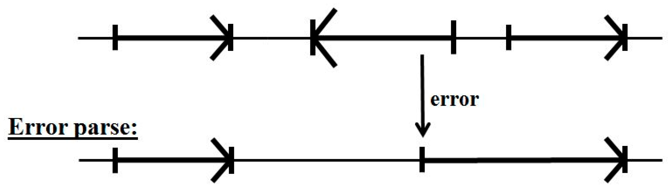
5.2. Impact of Annotation Errors
6. Conclusions
Supplementary Materials
Acknowledgments
Author Contributions
Conflicts of Interest
References
- Stanke, M.; Morgenstern, B. AUGUSTUS: A web server for gene prediction in eukaryotes that allows user-defined constraints. Nucleic Acids Res. 2005, 33, W465–W467. [Google Scholar] [CrossRef] [PubMed]
- Rajapakse, J.C.; Ho, L.S. Markov Encoding for Detecting Signals in Genomic Sequences. IEEE/ACM Trans. Comput. Biol. Bioinform. 2005, 2, 131–142. [Google Scholar] [CrossRef] [PubMed]
- Majoros, W.H.; Pertea, M.; Salzberg, S.L. TigrScan and GlimmerHMM: Two open source ab initio eukaryotic gene-finders. Bioinformatics 2004, 1, 2878–2879. [Google Scholar] [CrossRef] [PubMed]
- Taher, L.; Rinner, O.; Garg, S.; Sczyrba, A.; Brudno, M.; Batzoglou, S.; Morgenstern, B. AGenDA: Homology-based gene prediction. Bioinformatics 2003, 19, 1575–1577. [Google Scholar] [CrossRef] [PubMed]
- Altschul, S.F.; Gish, W.; Miller, W.; Myers, E.W.; Lipman, D.J. Basic local alignment search tool. J. Mol. Biol. 1990, 215, 403–410. [Google Scholar] [CrossRef]
- Sonnenburg, S.; Zien, A.; Ratsch, G. ARTS: Accurate recognition of transcription starts in human. Bioinformatics 2006, 22, e472–e480. [Google Scholar] [CrossRef] [PubMed]
- Do, J.H.; Choi, D.-K. Computational Approaches to Gene Prediction. J. Microbiol. 2006, 44, 137–144. [Google Scholar] [PubMed]
- Korf, I. Gene finding in novel genomes. BMC Bioinform. 2004, 5, 59. [Google Scholar] [CrossRef] [PubMed] [Green Version]
- Mathe, C.; Sagot, M.-F.; Schiex, T.; Rouze, P. Current methods of gene prediction, their strengths and weaknesses. Nucleic Acids Res. 2002, 30, 4103–4117. [Google Scholar] [CrossRef] [PubMed]
- Allen, J.E.; Majoros, W.H.; Pertea, M.; Salzberg, S.L. JIGSAW, GeneZilla, and GlimmerHMM: Puzzling out the features of human genes in the ENCODE regions. Genome Biol. 2006, 7 (Suppl. 1), S9. [Google Scholar] [CrossRef] [PubMed]
- Winters-Hilt, S.; Baribault, C. A Meta-state HMM with application to gene structure identification in eukaryotes. EURASIP J. Adv. Signal Process. 2010, 2010, 581373. [Google Scholar] [CrossRef]
- Winters-Hilt, S.; Jiang, Z. A hidden Markov model with binned duration algorithm. IEEE Trans. Signal Proc. 2010, 58, 948–952. [Google Scholar] [CrossRef]
- Winters-Hilt, S.; Jiang, Z.; Baribault, C. Hidden Markov model with duration side-information for novel HMMD derivation, with application to eukaryotic gene finding. EURASIP J. Adv. Signal Process. 2010, 2010, 761360. [Google Scholar] [CrossRef]
- Noguchi, H.; Park, J.; Takagi, T. MetaGene: Prokaryotic gene finding from environmental genome shotgun sequences. Nucleic Acids Res. 2006, 34, 5623–5630. [Google Scholar] [CrossRef] [PubMed]
- Kulp, D.; Haussler, D.; Reese, M.G.; Eeckman, F.H. A generalized hidden Markov model for recognition of human genes in DNA. Proc. Int. Conf. Intell. Syst. Mol. Biol. 1996, 4, 134–142. [Google Scholar] [PubMed]
- Van Baren, M.J.; Koebbe, B.C.; Brent, M.R. Using N-SCAN or TWINSCAN to predict gene structures in genomic DNA sequences. Curr. Protoc. Bioinform. 2007. [Google Scholar] [CrossRef]
- Rogic, S.; Mackworth, A.K.; Francis Ouellette, B.F. Evaluation of Gene-Finding Programs on Mammalian Sequences. Genome Res. 2001, 11, 817–832. [Google Scholar] [CrossRef] [PubMed]
- Dunham, I.; Shimizu, N.; Roe, B.A.; Chissoe, S. The DNA sequence of human chromosome 22. Nature 1999, 402, 489–495. [Google Scholar] [CrossRef] [PubMed]
- Burset, M.; Guigo, R. Evaluation of Gene Structure Prediction Programs. Genomics 1996, 34, 353–367. [Google Scholar] [CrossRef] [PubMed]
- Winters-Hilt, S.; Roux, B. Hybrid MM/SVM structural sensors for stochastic sequential data. In Proceedings of the Fifth Annual MCBIOS Conference. Systems Biology: Bridging the Omics, Oklahoma City, OK, USA, 23–24 February 2008. BMC Bioinform. 2008, 9 (Suppl. 9), S12. [Google Scholar]
- Liu, H.; Han, H.; Li, J.; Wong, L. DNAFSMiner: A Web-Based Software Toolbox to Recognize Two Types of Functional Sites in DNA Sequences. Available online: http://sdmc.i2r.a-star.edu.sg/DNAFSMiner/ (accessed on 26 June 2016).
- Sonnenburg, S.; Schweikert, G.; Philips, P.; Behr, J.; Rätsch, G. Accurate splice site prediction using support vector machines. BMC Bioinform. 2007, 8 (Suppl. 10), S7. [Google Scholar] [CrossRef] [PubMed]
- Degroeve, S.; Saeys, Y.; de Baets, B.; Rouzé, P.; van de Peer, Y. SpliceMachine: Predicting splice sites from high-dimensional local context representations. Bioinformatics 2005, 21, 1332–1338. [Google Scholar] [CrossRef] [PubMed]
- Muro, E.M.; Herrington, R.; Janmohamed, S.; Frelin, C.; Andrade-Navarro, M.A.; Iscove, N.N. Identification of gene 3’ ends by automated EST cluster analysis. PNAS 2008, 105, 20286–20290. [Google Scholar] [CrossRef] [PubMed]
- Bellora, N.; Farre, D.; Alba, M.M. PEAKS: Identification of regulatory motifs by their position in DNA sequences. Bioinformatics 2007, 23, 243–244. [Google Scholar] [PubMed]
- He, X.; Ling, X.; Sinha, S. Alignment and Prediction of cis-Regulatory Modules Based on a Probabilistic Model of Evolution. PLoS Comput. Biol. 2009, 5, 1–14. [Google Scholar] [CrossRef] [PubMed]
- Winters-Hilt, S.; Baribault, C. A novel, fast, HMM-with-Duration implementation—For application with a new, pattern recognition informed, nanopore detector. BMC Bioinform. 2007, 8 (Suppl. 7), S19. [Google Scholar] [CrossRef] [PubMed]
- Winters-Hilt, S. Hidden Markov Model Variants and their Application. BMC Bioinform. 2006, 7 (Suppl. 2), S14. [Google Scholar] [CrossRef] [PubMed]
- Lu, D. Motif Finding. Master Thesis, University of New Orleans, New Orleans, LA, USA, 2009. [Google Scholar]
- Shinozaki, D.; Akutsu, T.; Maruyama, O. Finding optimal degenerate patterns in DNA sequences. Bioinformatics 2003, 19 (Suppl. 2), ii206–ii214. [Google Scholar] [CrossRef] [PubMed]
- Frickey, T.; Weiller, G. Mclip: Motif detection based on cliques of gapped local profile-to-profile alignments. Bioinformatics 2007, 23, 502–503. [Google Scholar] [CrossRef] [PubMed]
- De Hoon, M.J.L.; Imoto, S.; Nolan, J.; Miyano, S. Open source clustering software. Bioinformatics 2004, 20, 1453–1454. [Google Scholar] [CrossRef] [PubMed]
- Wang, G.; Yu, T.; Zhang, W. WordSpy: Identifying transcription factor binding motifs by building a dictionary and learning a grammar. Nucleic Acids Res. 2005, 33, W412–W416. [Google Scholar] [CrossRef] [PubMed]
- Durbin, R.; Eddy, S.; Krogh, A.; Mitchison, G. Biological Sequence Analysis, Probabilistic Models of Proteins and Nucleic Acids; Cambridge University Press: Cambridge, UK, 1998. [Google Scholar]
- Rabiner, L.R.; Juang, B.H. An Introduction to Hidden Markov Models. IEEE ASSP Mag. 1986, 3, 4–16. [Google Scholar] [CrossRef]
- Winters-Hilt, S. Machine-Learning Based Sequence Analysis, Bioinformatics & Nanopore Transduction Detection; Lulu.com Publishing: Chapel Hill, NC, USA, 2011. [Google Scholar]


| Species | Release | GTF File |
|---|---|---|
| Human (Homo sapiens) | 75 | Homo_sapiens.GRCh37.75.gtf |
| Mouse (Mus musculus) | 81 | Mus_musculus.GRCm38.81.gtf |
| Worm (Caenhorhabditis elegans) | 83 | Caenhorhabditis_elegans.WBcel235.83.gtf |
| Fly (Drosophila melanogaster) | 75 | Drosophila_melanogaster.BDGP5.75.gtf |
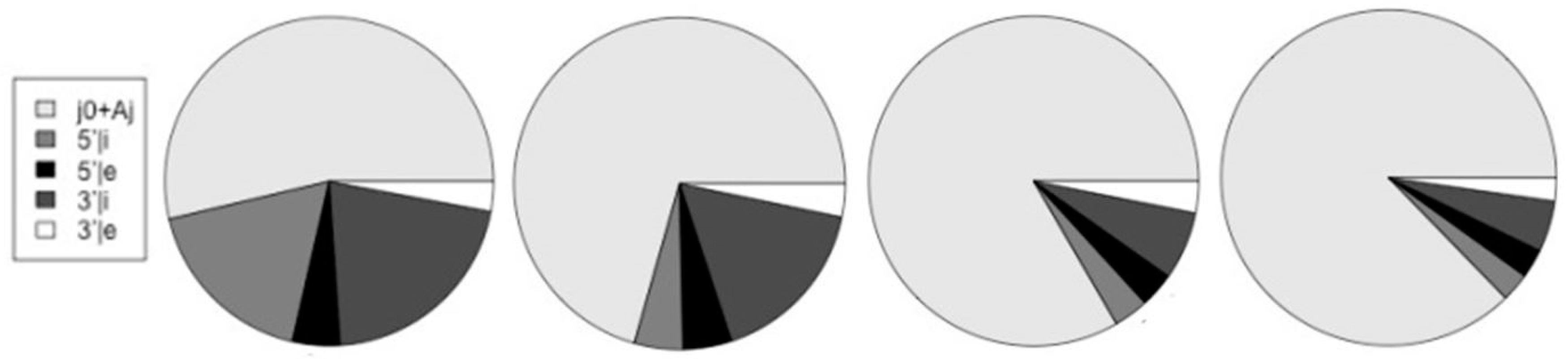
| Species | j0+Aj | 5’|i | 5’|e | 3’|i | 3’|e | altsum | Alt/j0 |
|---|---|---|---|---|---|---|---|
| Worm | 25,462 | 809 | 809 | 1,438 | 653 | 4,283 | 0.175 |
| Fly | 18,730 | 768 | 768 | 1,501 | 699 | 4,385 | 0.234 |
| Mouse | 33,561 | 2,260 | 2,260 | 7,922 | 1,540 | 18,473 | 0.550 |
| Human | 36,620 | 12,075 | 3,186 | 14,317 | 2,002 | 31,580 | 0.862 |
| V-trans | Human | Mouse | Fly | Worm |
|---|---|---|---|---|
| H-trans j0 | 18,911 | 16,899 | 9,389 | 12,938 |
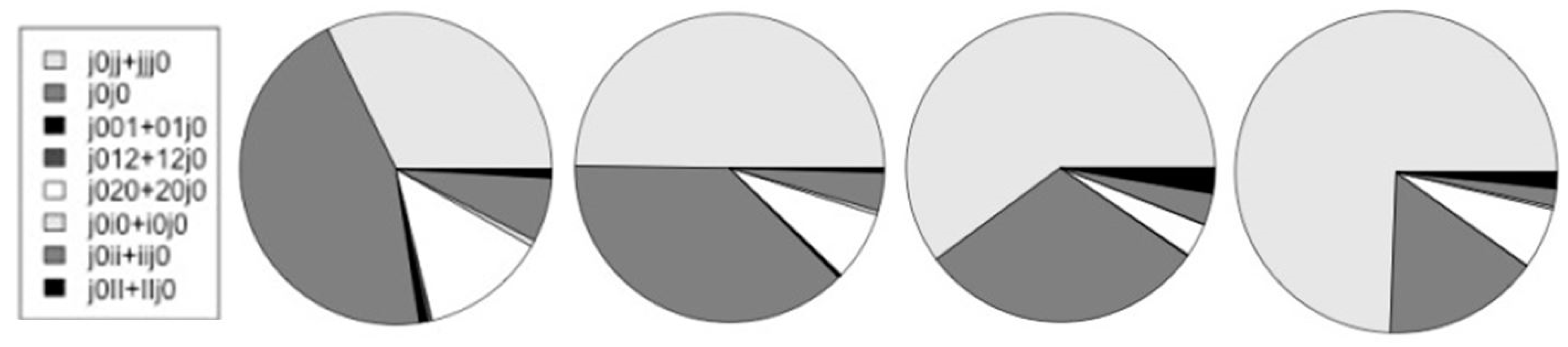
| {j0jj + jjj0} | 4,208 | 6,112 | 4,334 | 8,323 |
| j0j0 | 5,892 | 4,623 | 2,178 | 1,750 |
| {j001 + 01j0}* | 106 | 32 | 10 | 4 |
| {j012 + 12j0}* | 65 | 14 | 0 | 2 |
| {j020 + 20j0}* | 1,695 | 888 | 251 | 686 |
| {j0i0 + i0j0}* | 88 | 55 | 6 | 32 |
| {j0ii + iij0} | 873 | 490 | 237 | 204 |
| {j0II + IIj0} | 118 | 59 | 193 | 181 |
| {j0jj + jjj0}/j0 | 0.223 | 0.362 | 0.462 | 0.643 |
| */non-* | 0.176 | 0.088 | 0.038 | 0.069 |
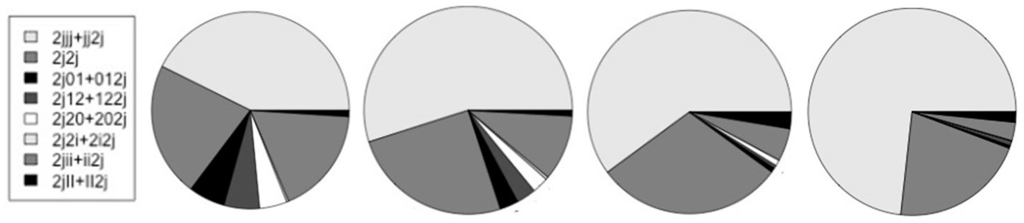
| V-trans | Human | Mouse | Fly | Worm |
|---|---|---|---|---|
| H-trans 2j | 19,040 | 16,727 | 9,409 | 12,955 |
| {2jjj + jj2j} | 6,641 | 7,347 | 4,355 | 7,843 |
| 2j2j | 3,442 | 3,359 | 2,163 | 2,249 |
| {2j01 + 012j}* | 926 | 383 | 48 | 46 |
| {2j12 + 122j}* | 908 | 406 | 39 | 79 |
| {2j20 + 202j}* | 704 | 339 | 70 | 5 |
| {2j2i + 2i2j}* | 51 | 55 | 0 | 3 |
| {2jii + ii2j} | 2,749 | 1,371 | 378 | 306 |
| {2jII + II2j} | 156 | 117 | 192 | 175 |
| {2jjj + jj2j}/2j | 0.349 | 0.439 | 0.463 | 0.605 |
| */non-* | 0.199 | 0.097 | 0.022 | 0.013 |
© 2017 by the authors; licensee MDPI, Basel, Switzerland. This article is an open access article distributed under the terms and conditions of the Creative Commons Attribution (CC BY) license ( http://creativecommons.org/licenses/by/4.0/).
Share and Cite
Winters-Hilt, S.; Lewis, A.J. Alt-Splice Gene Predictor Using Multitrack-Clique Analysis: Verification of Statistical Support for Modelling in Genomes of Multicellular Eukaryotes. Informatics 2017, 4, 3. https://doi.org/10.3390/informatics4010003
Winters-Hilt S, Lewis AJ. Alt-Splice Gene Predictor Using Multitrack-Clique Analysis: Verification of Statistical Support for Modelling in Genomes of Multicellular Eukaryotes. Informatics. 2017; 4(1):3. https://doi.org/10.3390/informatics4010003
Chicago/Turabian StyleWinters-Hilt, Stephen, and Andrew J. Lewis. 2017. "Alt-Splice Gene Predictor Using Multitrack-Clique Analysis: Verification of Statistical Support for Modelling in Genomes of Multicellular Eukaryotes" Informatics 4, no. 1: 3. https://doi.org/10.3390/informatics4010003