On Exactitude in Financial Regulation: Value-at-Risk, Expected Shortfall, and Expectiles


1
College of Law, Michigan State University, 648 North Shaw Lane, East Lansing, MI 48824-1300, USA
2
Visiting Scholar, School of Economics and Business, University of Zagreb (Ekonomski Fakultet, Sveučilište u Zagrebu), J.F. Kennedyja Trg 6, 10000 Zagreb, Croatia
Risks 2018, 6(2), 61; https://doi.org/10.3390/risks6020061
Submission received: 8 April 2018
/
Revised: 24 May 2018
/
Accepted: 28 May 2018
/
Published: 1 June 2018
Abstract
:This article reviews two leading measures of financial risk and an emerging alternative. Embraced by the Basel accords, value-at-risk and expected shortfall are the leading measures of financial risk. Expectiles offset the weaknesses of value-at-risk (VaR) and expected shortfall. Indeed, expectiles are the only elicitable law-invariant coherent risk measures. After reviewing practical concerns involving backtesting and robustness, this article more closely examines regulatory applications of expectiles. Expectiles are most readily evaluated as a special class of quantiles. For ease of regulatory implementation, expectiles can be defined exclusively in terms of VaR, expected shortfall, and the thresholds at which those competing risk measures are enforced. Moreover, expectiles are in harmony with gain/loss ratios in financial risk management. Expectiles may address some of the flaws in VaR and expected shortfall—subject to the reservation that no risk measure can achieve exactitude in regulation.
1. Introduction
Quantifying market risk represents the first step toward cogent financial management and regulation. The design of risk measures, however, presents its own hazards (Barrieu and Scandolo 2015). Model risk subsists in the specification, validation, and implementation of any risk measure (Kellner and Rösch 2016, pp. 45–47; Derman 1996). Errors in describing or estimating the distribution of losses can profoundly affect the accuracy of a risk measure (Gourieroux et al. 2000). “Broadly speaking, model risk can be attributed to either an incorrect model or to an incorrect implementation of a model” (Buraschi and Corielle 2005, p. 2884).
Global standards for banking regulation are peculiarly susceptible to model risk. The Basel Committee on Banking Supervision recognizes three types of model risk: “conceptual methodology, parameter specification and estimation, and validation” (BCBS 1999, p. 4). Failure in any of these respects may exacerbate economic hazards in an enterprise already fraught with peril.
Two measures of market risk dominate contemporary financial regulation. Since its adoption by Basel II in 1996, value-at-risk (VaR) has become the most widely used measure of financial risk. Among other drawbacks, however, VaR fails to satisfy mathematical principles characterizing coherent risk measures. In addition to ignoring losses beyond a designated threshold, VaR lacks subadditivity.
In 2013, Basel III proposed an alternative risk measure. Expected shortfall is theoretically coherent and quantifies tail risk. Nevertheless, expected shortfall fails a different mathematical principle: the elicitability criterion deemed essential to backtesting.
These deficiencies have heightened interest in a third approach. Expectiles represent the lone class of law-invariant, coherent, and elicitable risk measures. Although some sources characterize expectiles as opaque and deficient in intuitive appeal, the theoretical case favoring expectiles compels a closer look (Ziegel 2016, p. 916).
The quest for a “best” risk measure in practice often forces banks to pick one measure and one numerical result (Emmer et al. 2015, p. 41). Nevertheless, the regulation of market risk does not categorically foreclose the simultaneous application of multiple measures. In particular, the recognition that expected shortfall is jointly elicitable with VaR suggests that proper modeling may require several distinct but intellectually consilient measures of risk.
The financial academy bears a “crucial” responsibility to review and anticipate “changes in the regulatory landscape” and to inform “regulatory and industry practice” (Embrechts et al. 2014, p. 26). This article seeks to advance that mission by clarifying theoretical and practical issues affecting the design, testing, and implementation of VaR, expected shortfall, and expectiles.
Section 2 and Section 3 introduce VaR and expected shortfall as the leading risk measures in financial regulation. Section 2 describes VaR and its failure to satisfy the theoretical definition of a coherent risk measure. Section 3 describes expected shortfall and its own theoretical shortcoming: the failure to be elicitable.
Section 4 distinguishes between traditional and comparative backtesting. Passing traditional backtests such as those prescribed by Basel III is a necessary step for a risk measure, but not sufficient on its own. Section 5 discusses robustness as a qualitative property that exposes tradeoffs, such as the balance between subadditivity and sensitivity.
Section 6 introduces expectiles and their mathematical properties as a special class of quantiles. Section 7 defines expectiles exclusively in terms of VaR, expected shortfall, and those competing risk measures’ regulatory thresholds. Section 8 describes expectiles in terms of the ratio between upside gain and downside loss. Section 9 concludes that expectiles may ease some of the tension between VaR and expected shortfall—subject to the reservation that no risk measure can achieve exactitude in regulation.
2. Value-at-Risk and Coherence
In the most general terms, a “risk measure is a mapping from the set of random variables representing investment results to … real numbers” (Chen and Hu 2017, p. 1). Both value-at-risk and expected shortfall are law-invariant risk measures (Kusuoka 2001), since both measures depend solely on the distribution of losses. If “Z and Z′ are two distributionally equivalent random variables”, then the application of a law-invariant risk measure reports equivalent risk: (Shapiro 2013, p. 142). Law-invariant measures “are of special interest” in financial regulation because their values “depend only on the distribution of losses” and estimation requires “no additional information such as stress scenarios” (Emmer et al. 2015, p. 35).
VaR and expected shortfall, however, each lack an essential mathematical property. VaR flunks the requirements demanded of coherent risk measures. By curing VaR’s lack of subadditivity, expected shortfall is coherent. For its part, expected shortfall fails to satisfy elicitability, a property associated with effective backtesting. Expectiles combine the elicitability of VaR with the coherence of expected shortfall. Indeed, expectiles are the only law-invariant risk measures that are both coherent and elicitable.
The balance of Section 2 discusses VaR and coherence. Section 3 addresses expected shortfall and introduces the concept of elicitability.
2.1. Value-at-Risk
Let Y represent a financial position expressed as a random variable real number. Formally, value-at-risk describes the upper threshold of the interval of losses (–∞, zα] randomly occurring within fY(x), the probability density function of the distribution of returns on Y, at threshold α ∈ (0, 1) (Daníelsson and Zigrand 2006, p. 2702, n. 1):
VaR may also be defined in terms of the corresponding cumulative distribution function FY(x) (Ziegel 2016, p. 901; Nolde and Ziegel 2017a, p. 1835):
As a quantile (Duffie and Pan 1997), VaR may be expressed directly in terms of the inverse cumulative distribution function: .
Many sources, including official publications of the Basel Committee on Bank Supervision, speak of VaR and expected shortfall in terms of confidence level 1 – α rather than the probabilistic threshold α. Throughout this article, levels of VaR and expected shortfall designated according to confidence level 1 – α will be indicated by the subscript CL: VaRCL=0.99 or ESCL=0.975. Risk measures so designated indicate positive distance from the right tail of a distribution of losses.
For normally distributed risk, , VaRα corresponds to the probit function, . At α = 0.01, . Parametric VaR “generalizes to other distributions as long as all the uncertainty is contained in σ” (Jorion 2006, p. 113). Nonparametric and semiparametric methods for computing VaR abound (Manganelli and Engle 2004, p. 124).
VaR remains “the most widespread risk measure in the banking and insurance sectors” (Bellini and Bignozzi 2015, p. 725). The original RiskMetrics specification is available on a nonproprietary basis (Mina and Xiao 2001). Although “Gaussian assumptions are not realistic in finance” (Righi and Ceretta 2015, p. 17), RiskMetrics erroneously assumes that returns are normally distributed (Pafka and Kondor 2001). Basel II adopted a version of VaR as its preferred risk measure (BCBS 1996, 2004). The current accord, Basel III, prescribes VaRCL=0.99 (BCBS 2013, pp. 103–8), a value that should be regarded as the global standard (Nolde and Ziegel 2017a, p. 1835).
2.2. Subadditivity, Coherence, and Comonotonicity
VaR, however, may be as contested as it is popular (Acerbi 2002). VaR’s theoretical flaws present a deep source of model risk in financial regulation (Dowd and Blake 2006). Risk measure ρ, as applied to positions Y, Y1, and Y2, is coherent if and only if it satisfies all of these conditions (Artzner et al. 1999):
- Translation (drift) invariance: Adding a constant return c to total return will reduce risk by that amount: .
- (Linear) homogeneity: Multiplying any position by positive factor λ results in a corresponding, linear increase in risk: .
- Monotonicity: If position Y1 is first-order stochastically dominant to position Y2, in that Y1 offers higher returns than Y2 in every conceivable economic state (Levy 1992, 2015), then the risk associated with Y1 cannot exceed the risk associated with Y2: . Y1 dominates Y2 in the sense that —i.e., the cumulative distribution function of losses for Y1 is less than or equal to the cdf for Y2 for all x. Therefore, .
- Subadditivity: The risk associated with two combined positions cannot exceed the total risk associated with either position, considered alone: .
VaR satisfies translation invariance, linear homogeneity, and monotonicity. However, VaR flunks the subadditivity criterion. VaR not only “completely ignore[s] the severity of losses in the far tail of the loss distribution,” but also “lack[s] … the subadditivity property” (Emmer et al. 2015, p. 39). VaR’s failure to satisfy subadditivity is particularly troubling when financial positions comprise distinct subcomponents, each amenable to its own evaluation of market risk (Hull 2015, pp. 260–62).
Failing to be subadditive gives rise to “the surprising property that the VaR of a sum may be higher than the sum of the VaRs” for each component of a financial portfolio (Daníelsson 2004, pp. 26–27). VaR’s non-subadditivity invites financial institutions to assemble “portfolios that are very concentrated and … quite risky by normal economic standards” (McNeil et al. 2005, p. 239). VaR’s failure to properly measure the benefits of diversification exposes its practical limitations (Emmer et al. 2015, p. 51). As the number of positions increases, VaR deceptively overreports the diversification benefit (Busse et al. 2014).
Non-subadditive VaR scores might tempt banks “to legally break up into various subsidiaries in order to reduce … regulatory capital requirements” (Emmer et al. 2015, p. 73). Wholly apart from diversification, subadditivity neutralizes regulatory arbitrage (Osband 2011, pp. 25, 75, 114). Providing proper incentives to forecast risk accurately remains an important goal in financial regulation (Nolde and Ziegel 2017a, p. 1834; Nolde and Ziegel 2017b, pp. 1906, 1908).
“[F]or many practical applications,” VaR’s lack of subadditivity is manageable “as long as the underlying risks have a finite variance or, in some cases, a finite mean” (Emmer et al. 2015, p. 56). Substituting semiparametric extreme value techniques for historical simulations can reduce violations of subadditivity (Daníelsson et al. 2013). Furthermore, subadditive risk measures may inadvertently raise post-merger shortfall risk, thereby discouraging otherwise efficient transactions (Dhaene et al. 2008; Kou et al. 2013, p. 405). All of these considerations undermine the value of coherence (Cont et al. 2010, p. 604).
3. Expected Shortfall and Elicitability
3.1. Expected Shortfall as a Response to VaR
As early as 2011, the Basel Committee on Banking Supervision acknowledged the failure of VaR to satisfy coherence (BCBS 2011b, pp. 17–20). In 2012, the Basel Committee proposed phasing out VaR (BCBS 2012, p. 20). In 2013, the Committee ultimately recognized numerous “weaknesses … in using Value-at-Risk (VaR) for determining regulatory capital requirements, including its inability to capture tail risk” (BCBS 2013, p. 3). It adopted expected shortfall at a confidence level of 97.5 percent, “a broadly similar level of risk capture as the 99th percentile VaR threshold” (ibid., p. 18; see also BCBS 2014, pp. 14, 19). Daníelsson et al. (2013, p. 283) detected higher volatility in ESCL=0.975 forecasts relative to VaRCL=0.99.
Expected shortfall—also known as average VaR, conditional VaR, or tail conditional expectation (Rockafellar and Uryasev 2000, 2002)—is a transformation of VaRα for position Y (Nolde and Ziegel 2017a, p. 1835; Ziegel 2016, p. 901):
Whereas VaR at threshold α assigns zero weight to all other quantiles, expected shortfall assigns equal weight to all quantiles below α (Hull 2015, p. 263).
By analogy to VaR, expected shortfall may be expressed through integration of the inverse cumulative distribution function:
Equivalently, where , expected shortfall may be expressed through integration of the probability distribution function, fY(x):
For normally distributed risk, , ESα is the definite integral of the probit function, , for p = 0 to α, divided by α. Expected shortfall at α = 0.025 is ESα = (ibid., p. 294). As Basel III’s adoption of a 97.5 percent confidence level for expected shortfall suggests (BCBS 2013), normally distributed ESCL=0.975 ≈ 2.337808 approximates the risk level at VaRCL=0.99 ≈ −2.326348.
Expected shortfall redresses VaR’s disregard for the shape and size of the distribution beyond a designated quantile (Yamai and Yoshiba 2002, pp. 65–80). By reporting “the mean loss when the loss … exceeds the VaR level,” expected shortfall “gives an estimate of the amount of capital depreciated under worst-case scenarios that are quantified by VaR” (So and Wong 2012, p. 739). Because expected shortfall satisfies law-invariance (Kusuoka 2001; Shapiro 2013) and comonotonic additivity (Embrechts et al. 2002) in addition to the four conditions demanded of coherent risk measures (Acerbi and Tasche 2002; Inui and Kijima 2005), it fulfills all six of the conditions that define spectral risk measures (Acerbi 2002; Dowd et al. 2008; Fuchs et al. 2017, pp. 7–12).
Spectral risk measures support closed-form solutions to worst-case estimates as long as the first two moments of the return distribution are known (Li 2017). This finding extends a known trait of VaR (El Ghaoui et al. 2003; Ye et al. 2012) and expected shortfall (Chen et al. 2011; Natarajan et al. 2010). Adjusting portfolio weights enables spectral risk measures to accommodate subjective risk aversion (Acerbi 2002; Adam et al. 2008; Cotter and Dowd 2006).
3.2. Elicitability
On its own, however, “theoretical appeal” cannot overcome the “major drawbacks to using spectral risk measures in risk management” (Ziegel 2016, p. 902). The Basel Committee momentarily described “[s]pectral risk measures [as] a promising generalization” of expected shortfall (BCBS 2012, p. 60). Not surprisingly, that claim tdisappeared from Basel’s 2013 consultative document on market risk (BCBS 2013).
The central problem in validating VaR, expected shortfall, or any other law-invariant risk measure is that the “distribution function of the financial position” is “usually unknown” in principle and must be estimated in practice from a limited “sample of available data” (Bellini and Bignozzi 2015, p. 726; see also Cont et al. 2010, p. 593). Backtesting “refers to validating a given estimation procedure for a risk measure on historical data” (Ziegel 2016, p. 902). The “comparison of realized losses with risk measure forecasts” over time evaluates the “performance of a (trading book) risk measurement procedure” (Nolde and Ziegel 2017a, p. 1834).
All three steps in harmonizing a theoretical model with data—estimation, backtesting, and forecast verification (Escanciano and Olmo 2011; Ziegel 2016, p. 902)—assume greater significance in light of Basel 2.5’s addition of “stressed VaR” (BCBS 2011a; see also Blundell-Wignall and Atkinson 2010; Chen 2014, pp. 191–92; Escanciano and Pei 2012, p. 2233 and note 1; Rossignolo et al. 2012). Stressed VaR subjects VaRCL=0.99 to a one-year historic dataset spanning “a continuous 12-month period of significant financial stress” (BCBS 2011a, p. 2).
Forecasts of future quantities or events should be probabilistic in nature, taking the form of predictive probability distributions (Gneiting 2008; Gneiting and Katzfuss 2014). Tradition or perceived ease in communication, however, often favors single-point estimates (Ehm et al. 2016, pp. 505–6; Gneiting 2011, p. 746). Financial risk measures therefore represent a special instance of evaluating “single-valued point forecast[s]” as though such estimates themselves took the “form of probability distributions over future quantities or events” (Gneiting 2011, p. 746).
A scoring function “compare[s] and assesse[s]” competing forecast cases according to “both … the forecast and the realization” by comparing “point forecasts, x1, …, xn [with] verifying observations, y1, …, yn” (ibid.):
Common scoring functions include squared error, absolute error, absolute percentage error, and relative error (Patton 2011). The proliferation of scoring functions without consensus on basic requirements (Fildes et al. 2008, p. 1158) crippled the “science of forecast verification” (Murphy and Winkler 1987, p. 1330). Asking forecasters to predict “real-valued outcomes such as firm profit, GDP, growth, or temperature” without “explicit guidance” invites reliance upon “subjective means, … medians or modes” (Engelberg et al. 2009, p. 30).
The resulting practice of “evaluating … forecasters” according to “some” arbitrary scoring function “is not a meaningful endeavor” (Gneiting 2011, p. 748). The application of scoring functions such as absolute, relative, or squared error can favor “ignorant no-change forecast[s]” over “skilful statistical forecasts” (Ziegel 2016, p. 904). It is jarring and counterintuitive for a scoring function to prefer an arbitrary, constant prediction over thoughtful statistical analysis, simply because the thoughtless forecast registers a lower squared error or relative error (Gneiting 2011, p. 747).
Elicitability imposes conditions on scoring functions (Gneiting 2011, p. 749):
- “Let the interval I be the potential range of the outcomes, … and let the probability distribution F be concentrated on I.”
- “Then a scoring function is any mapping S: I × I → [0, ∞).”
- “A functional is a potentially set valued mapping .”
- “A scoring function S is consistent for the functional T if for all F, all t ∈ T(F) and all x ∈ I.”
- The scoring function S “is strictly consistent if it is consistent and equality of the expectations implies that x ∈ T(F).”
- Therefore, “a functional is elicitable if there exists a scoring function that is strictly consistent for it.”
See also Bellini and Bignozzi (2015, p. 725); Ehm et al. (2016, pp. 508–9); Nolde and Ziegel (2017a, p. 1836); Ziegel (2016, pp. 904–5). “[E]licitability is a key property for a risk measure [inasmuch] as it provides a natural methodology to perform backtesting” (Bellini and Bignozzi 2015, p. 726).
3.3. The Nonelicitability of Expected Shortfall
One of the iconic instances of elicitability has profound regulatory implications. VaR takes the form of an “α-quantile (0 < α < 1) of the cumulative distribution F,” or “any number x for which ” (Gneiting 2011, p. 754; see also Duffie and Pan 1997). The “α-quantile functional is elicitable relative to” the “class of probability measures on the interval I ⊆ ℜ” (Gneiting 2011, p. 754). Since VaR is a quantile, it is elicitable (Ziegel 2016, p. 905). “Subject to some regularity and integrability conditions” (ibid.), a scoring function S “is consistent for the α-quantile … on [interval] I if, and only if, it is of the form, , where g is a nondecreasing function on I” and 1A denotes the indicator function (Gneiting 2011, p. 755; accord Bellini and Bignozzi 2015, p. 726; Nolde and Ziegel 2017a, p. 1837; Ziegel 2016, p. 905).
Weber (2006, pp. 429–30) appears to have been the first to recognize the non-elicitability of expected shortfall (accord Bellini and Bignozzi 2015, p. 730; Ziegel 2016, p. 902). Gneiting (2011, p. 756) flatly declared expected shortfall to be not elicitable. Nonelicitability may partially explain expected shortfall’s “difficulties with robust estimation and backtesting” (Ziegel 2016, p. 902). In contrast with the deep literature on forecasting with VaR and other quantiles (Bao et al. 2006; Berkowitz et al. 2011; Berkowitz and O’Brien 2002; Escanciano and Olmo 2011; Giacomini and Komunjer 2005; Kuester et al. 2006; Kupiec 1995; Mabrouk and Saadi 2012; Małecka 2017), Gneiting (2011, p. 756) observed that the evaluation of expected shortfall forecasts lacked a comparable base of support.
Existing processes for backtesting expected shortfall (Christoffersen 2011, p. 308; Costanzino and Curran 2015; Du and Escanciano 2017, pp. 942–44; Kerkhof and Melenberg 2004; McNeil and Frey 2000, pp. 291–96) do not permit “a direct comparison and ranking of the predictive performance of competing forecasting models” (Gneiting 2011, p. 756). Implicitly backtesting expected shortfall by simultaneously testing several levels of VaR (Emmer et al. 2015, pp. 53–54; Kratz 2017; Kratz et al. 2018) establishes at best a “debatable” basis for backtesting expected shortfall (Nolde and Ziegel 2017b, p. 1902).
4. Backtesting
Difficulties with expected shortfall may arise not only from theoretical nonelicitability, but also from practical considerations. Backtesting expected shortfall is more difficult than backtesting VaR (Righi and Ceretta 2015, p. 15 and note 3). Indeed, it subsumes VaR backtesting inasmuch as “ES estimation … is conditionally linked to “VaR estimation.” (ibid.; see generally Righi and Ceretta 2013).
The recognition that expected shortfall is jointly elicitable with VaR (Fissler and Ziegel 2016; Fissler et al. 2016; Taylor 2017, part 5.2, preprint pp. 4–5) has sparked interest in the backtesting of expected shortfall (Acerbi and Székely 2014; Costanzino and Curran 2015, 2018; Du and Escanciano 2017). Section 4 examines this literature on either side of the boundary between traditional and comparative backtests.
4.1. Traditional Backtesting
“[A]ny backtest that considers” whether a “risk measurement procedure is correct” is a traditional backtest (Nolde and Ziegel 2017a, p. 1840). A traditional backtest asks whether “the risk measurement procedure under consideration is making incorrect predictions” (ibid.). Basel outlines “a consistent approach for incorporating P&L attribution and backtesting” (BCBS 2013, p. 107).
The most celebrated traditional backtest is the “traffic light” model in Basel III’s supervisory framework (BCBS 1996; BCBS 2013, pp. 103–8). Basel’s traffic light model for VaRCL=0.99 rests on “the cumulative probability
of obtaining x or fewer breaches” for “fixed N and level α” (Costanzino and Curran 2018, p. 2):
The green, yellow, and red zones of Basel’s traffic light model are defined by the boundaries between green and yellow and between yellow and red. “The yellow zone begins” where “the probability of obtaining” a specific “number or fewer exceptions” out of N observations “equals or exceeds 95%” (BCBS 2013, p. 105). Basel uses the “true Binomial Null distribution … rather than the asymptotic Normal distribution” to compute relevant probabilities (Costanzino and Curran 2018, p. 2; see BCBS 2013, pp. 104–5). “For 250 observations, … five or fewer exceptions will be obtained 95.88% of the time when the true level of coverage is 99%” (BCBS 2013, p. 105). Since 95.88% exceeds 95%, “the yellow zone begins at five exceptions” where N = 250 (ibid.). “Similarly, the beginning of the red zone is defined as the point such that the probability of obtaining that number or fewer exceptions equals or exceeds 99.99%” (ibid.).
The number of exceedances and the resulting zone (green, yellow, red) affect Basel’s computation of the daily capital charge (Chang et al. 2011; McAleer et al. 2013a, 2013b). The charge is the higher of the previous day’s risk measure or the 60-business-day average, multiplied by 3 + k (BCBS 1996; Kerkhof and Melenberg 2004, p. 1852 and note 12):
Multiplying VaR by 3 + k is designed to offset errors in model implementation (McAleer et al. 2009, p. 620). As Table 1 shows, k ∈ [0, 1] is based on the number of exceedances within 250 business days (BCBS 1996, table 2, p. 15; Kerkhof and Melenberg 2004, table 1, p. 1853):
Notably, Basel penalizes only the number of violations and not their individual or cumulative magnitude (McAleer et al. 2009, p. 618). This trait invites banks to evaluate “the trade-off between expected capital requirements and the expected number of violations” (ibid.). The imposition of any regulatory risk measure leaves banks free to innovate with internal risk models, even while complying with regulatory standards (Colson et al. 2007).
Applying Costanzino and Curran (2015), Costanzino and Curran (2018, pp. 3–5) extend Basel’s traffic light approach for VaR to backtesting expected shortfall according to a revised “breach indicator” that accounts for “the severity of the breach (i.e., losses beyond the VaR level) and is a continuous variable rather than discrete” (ibid., p. 3). By analogy to the cumulative probability of VaR breaches (ibid.):
For any confidence level v, the boundary between traffic light categories—between green and yellow, or yellow and red—can be determined by inverting the equation that expresses the cumulative probability of exceedances (ibid., p. 4):
The yellow zone begins where v = 0.95. The red zone begins where v = 0.9999 (ibid.).
4.2. Comparative Backtesting
Traditional backtests, however, “are not suited to compare different risk estimation procedures, and may be insensitive to increasing information” (Nolde and Ziegel 2017a, p. 1834). To overcome this limitation, comparative backtesting pits a “standard” regulatory risk model against an “internal” alternative (ibid., p. 1848):
- : The internal model predicts at least as well as the standard model.
- : The internal model predicts at most as well as the standard model.
sets the baseline for evaluating whether a traditional backtest is “a correct model and estimation procedure” (ibid.). Since regulators cannot prudently endorse a backtest solely because alone cannot be rejected, comparative backtesting takes the further step of asking whether the second null hypothesis, , can be rejected (ibid.). explicitly targets “the type I error” of endorsing “an inferior internal model over an established standard model” (ibid.). Obviously, “comparative backtests necessitate an elicitable risk measure” (ibid., p. 1834).
Although both tasks can be expressed through intuitive traffic light models, traditional and comparative backtests ask strikingly distinct questions. Traditional backtests ask whether a risk measure satisfies some baseline, such as 95 or 99.99 percent confidence. Comparative backtests, by contrast, pit risk measures against each other.
In other words, the three zones in Basel III’s traffic light approach, or any other traditional backtesting system, “arise from the confidence level of the hypothesis test” (ibid., p. 1849). By contrast, the confidence level in the comparative backtesting method of Fissler et al. (2016) “is fixed a priori, and the zones” distinguish between “cases where there is enough evidence” to prefer one risk-testing model over another, and “cases where there is no clear evidence” (Nolde and Ziegel 2017a, p. 1849). Table 2 summaries these competing “traffic light” approaches.
The “choice of a risk measure” for regulatory or internal use follows the longstanding practice of weighing “theoretical considerations” against “practical implications” (Nolde and Ziegel 2017a, p. 1833). To select “a risk measure in practice,” regulators must survey “a panorama of the mathematical properties” of prospective measures, such as “VaR, ES and expectile,” and weigh each measure’s “advantages and disadvantages” (Emmer et al. 2015, p. 31). In Basel’s transition to expected shortfall, VaR’s “drawbacks motivated an axiomatic analysis of [competing] risk measures with desirable properties” (Weber 2006, p. 419, emphasis added).
The introduction of comparative backtesting shifts the calculus. It no longer suffices merely to backtest expected shortfall. Even if a traditional backtest finds that expected shortfall exceedances fall below some level, it remains uncertain whether ESCL=0.975 outperforms other risk measures. Comparative backtesting demonstrates whether a bank’s internal risk measure outperforms ESCL=0.975 under Basel.
Transitions between regulatory risk models involve a similar evaluation of alternatives to the incumbent. The displacement of VaR by expected shortfall between Basel II and III is the iconic example. In turn, a future Basel accord may replace expected shortfall with the joint vector Θ(VaR, ES) (Fissler et al. 2016), median shortfall (Embrechts et al. 2014, p. 43; Kou et al. 2013, p. 402), or expectile-based expected shortfall (Daouia et al. 2018; Gschöpf et al. 2015).
A future transition between legally prescribed risk models must observe the same terms by which banks compare their internal models to regulatory standards. In either setting, “the statistical significance of the comparative backtests can be summarized by means of traffic light matrices highlighting which methods pass or fail against a standard procedure, and when not enough evidence is available to make a conclusive statement” (Nolde and Ziegel 2017a, p. 1870).
Backtesting serves a dual function. First, backtesting enables managers to verify whether their models are properly gauging risk (Wong 2010, p. 526). Second, by enabling “regulators … to adjust the level of capital requirement” and to punish “poor … risk management,” backtesting motivates banks to keep improving their risk models (ibid.). The former purpose is fulfilled by traditional backtesting. The latter purpose is the domain of comparative backtesting.
5. Robustness: Realism and Tradeoffs in the Choice of a Risk Measure
Although the method for comparing internal risk measures against regulatory criteria may be the same as those for selecting a single regulatory standard, the stakes in these settings differ. “Internal risk measures are applied in the interest of an institution’s shareholders or managers, whereas external risk measures are used by regulatory agencies to maintain safety and soundness of the financial system” (Kou et al. 2013, p. 394). The imposition of a single risk measure on an entire industry counsels closer attention to robustness.
Robustness requires two conditions. First, a “risk measure is said to be robust if … it can accommodate model misspecification” (ibid., p. 400). Second, a robust risk measure “is insensitive to small changes in the data, i.e., small changes in all or large changes in a few of the samples” (ibid.).
There appears to be “a fundamental theoretical conflict between subadditivity and robustness of risk measurement procedures” (Ziegel 2016, p. 902). Focusing on expected shortfall, Cont et al. (2010, p. 595) identify a “conflict between the subadditivity of a risk measure and the robustness of its estimation procedure.” One “cannot achieve robust estimation … while preserving subadditivity” (ibid., p. 604).
The “measure of risk of an unacceptable position, once a reference, ‘prudent,’ investment instrument has been specified, [is] the minimum extra capital, which, invested in the reference instrument, makes the future value of the modified position become acceptable” (Artzner et al. 1999, p. 204). Financial regulation focuses on “the variability of the future value of a position, due to market changes or more generally to uncertain events,” without regard to “initial costs” as “determined from universally defined market prices” (ibid., p. 205).
Though the admittedly qualitative notion of robustness (Cont et al. 2010, p. 594) does permit quantitative measurement (Krätschmer et al. 2012, p. 36; 2014, pp. 272–73). Accurately indexing “qualitative robustness” may demonstrate “greater robustness in a sense that is mathematically precise” (Krätschmer et al. 2014, p. 273). Evaluating risk measures according “to different metrics” and distinguishing among “degrees of robustness” may “provide a better balance between tail sensitivity and robustness” (Ziegel 2016, p. 902). Krätschmer et al. (2012, 2014) define “a continuum of degrees of robustness, in contrast with the more traditional binary notion” (Bellini and Bignozzi 2015, p. 730).
The most obvious practical implication is a greater thirst for data in backtesting expected shortfall relative to VaR (Bellini and Bignozzi 2015, p. 726; Daníelsson 2011, pp. 88–89). It takes more data to validate expected shortfall than VaR at the same level of certainty (Yamai and Yoshiba 2005). The estimation of expected shortfall (Wong 2008) “will often be based on larger subsamples than the estimation of VaR” (Emmer et al. 2015, p. 44).
As with elicitability, robustness neutralizes expected shortfall’s theoretical advantages over VaR. Even more than non-subadditivity, VaR’s failure to cover tail risks beyond a particular confidence level is considered a grave fault (ibid., p. 56). This very property “ironically … makes VaR … more robust” (ibid.). Expected shortfall “was introduced precisely as a remedy to the lack of risk sensitivity of VaR” (ibid., p. 44). That sensitivity undermines the preferred risk measure of Basel III.
Some evidence points in the opposite direction. Nuanced measurement through a “refined notion of qualitative robustness” shows that “robustness is not lost entirely but only to some degree when Value at Risk is replaced by a coherent risk measure such as … Expected Shortfall” (Krätschmer et al. 2012, p. 36). Measures of dependence uncertainty (Embrechts et al. 2014, pp. 31–37) “show that VaR generally exhibits a larger spread” relative to expected shortfall, which “suggests that VaR is more sensitive to dependence uncertainty” and therefore less robust (Embrechts et al. 2015, p. 767).
There is nevertheless a “natural tradeoff between robustness and tail sensitivity in risk measurement” (Krätschmer et al. 2014, p. 273). The tradeoff between expected shortfall’s subadditivity, coherence, and sensitivity (on one hand) and VaR’s elicitability and robustness (on the other) injects model risk during the very periods that Basel addressed through stressed VaR (BCBS 2011a).
The “intuitive and … probably intended” effect of raising capital requirements through the replacement of VaR by expected shortfall raises model risk associated with expected shortfall through “a higher potential for regulatory arbitrage” (Kellner and Rösch 2016, p. 58). “The better distributions are to reproduce extreme events,” the more expected shortfall “will be exposed to model risk” through vulnerability to parameter misspecification and “a higher degree of variation in estimation results” (ibid). Because this tradeoff arises from “heaviness in the tails of the model’s distributions” (ibid.), “divergence in model risk … tends to increase during turmoil periods” (ibid., p. 47). Regulation becomes most fragile when financial conditions demand that it be most resilient (Daníelsson et al. 2016, pp. 84–85).
Robustness should influence choices among financial risk measures (Krätschmer et al. 2012, p. 36). Alongside elicitability and backtesting, a regulatory interest in robustness and the “design of robust risk estimation procedures requires … explicit” attention to “statistical estimation” (Cont et al. 2010, p. 604).
Indeed, robustness is arguably indispensable to the effective implementation of industry-wide risk measures (Kou et al. 2013, p. 401). An “external risk model” robust “with respect to underlying models and data” ensures that “different judges will reach similar conclusions when they implement it” (ibid.). Reliance on “internal models and private data” can mislead financial regulation in two ways (ibid.). First, “the data can be noisy, flawed, or unreliable” (ibid.). Simple miscalculation is troubling enough; the industry-wide use of complex internal models may facilitate regulatory arbitrage (Embrechts et al. 2014, p. 40).
The second source of uncertainty arises from the mathematics of modeling (Heyde and Kou 2004). Limitations on data make it hard to distinguishable certain statistical models (Kou et al. 2013, p. 401). Even after “5,000 observations, roughly 20 years of daily observations,” it remains “very difficult to distinguish between exponential-type and power-type tails” (ibid.).
The global financial system rests upon “soft law,” where authority stems not from the power to compel, but the ability to persuade (Brummer 2012). Regulation suffers if the tail behavior purportedly described by external models depends on subjective assumptions (Kou et al. 2013, p. 401). An “external risk measure must be ambiguous, stable, and capable of being implemented consistently,” without regard to idiosyncratic beliefs or models not shared across the industry (ibid.). Absent robustness in its measure of risk, a legal regime may demand very different levels of regulatory capital for institutions facing the same risk (ibid.).
6. Expectiles
6.1. The Appealing Properties of Expectiles
The “τ-expectile functional (0 < τ < 1) of a probability measure F with finite mean as the unique solution x = µτ to [this] equation” (Gneiting 2011, p. 756):
Newey and Powell (1987) described µ(τ) as “determined by the properties of the expectation of the random variable Y,” whose cumulative distribution function is F(y), “conditional on Y being in a tail of the distribution” (ibid., p. 823). The “expectile function µ(τ) summarizes the distribution function in much the same way as the quantile function,” q(α) = F–1(α) (ibid.). The word expectile thus represents a linguistic portmanteau of expectation and quantile (Bellini and Di Bernardino 2017, p. 487).
“Expectiles generalize the expectation just as quantiles generalize the median” (Nolde and Ziegel 2017a, p. 1835). Specifically, “the 0.5-expectile is the mean …, while the 0.5-quantile is the median” (Jones 1994, p. 149)—provided that “the mean exists and … the median is uniquely defined” (Abdous and Rémillard 1995, p. 374).
Academic interest in expectiles addresses theoretical weaknesses in VaR and expected shortfall. Weber (2006, p. 433) showed that a loss function taking the form is coherent, as long as . The resulting “shortfall risk measure is equal to minus the τ-expectile,” µ(τ), where (Ziegel 2016, p. 903; see also Bellini and Bignozzi 2015, p. 733). However, Weber did not connect his work to Newey and Powell (1987) or later literature (Ziegel 2016, p. 903). Kuan et al. (2009) first proposed the use of expectiles as a financial risk measure (Ziegel 2016, p. 903).
Theoretical work on elicitability, in turn, appears to have spurred interest in expectiles as an alternative to expected shortfall. Despite hailing expected shortfall’s “elegant and appealing properties including coherency,” Gneiting (2011) recognized that expected shortfall “is not elicitable” (p. 756). Gneiting simultaneously acknowledged that the “τ-expectile functional is elicitable” (ibid., p. 755).
Subsequent work has confirmed the theoretical uniqueness of expectiles as the lone class of risk measures combining coherence (which eludes VaR) with elicitability (which eludes expected shortfall). “Expectiles are the only elicitable coherent risk measures” (Ziegel 2016, p. 903). More precisely, expectiles are the only generalized quantiles that are coherent risk measures, as long as τ ≤ ½ (Bellini et al. 2014, p. 45; Embrechts et al. 2014, p. 42; Ziegel 2016, p. 910). “The only elicitable law-invariant coherent risk measures are τ-expectiles for τ ∈ (0, ½]” (Ziegel 2016, p. 911, Corollary 4.6) Addressing a question that Ziegel (2016) allegedly left open—whether expectiles “are the unique coherent risk measure that is elicitable”—Bellini and Bignozzi (2015, p. 726) concluded, under some modifications, “that expectiles are indeed the only elicitable coherent risk measure.”
These theoretical properties “highlight the central role played by expectiles and … provide a further motivation for their study” (ibid., p. 733). At a minimum, the expectile-based analog of VaR “is a perfectly reasonable risk measure, displaying many similarities with VaRα and ESα, surely worthy of deeper study and practical experimentations” (Bellini and Di Bernardino 2017, p. 489). Regulatory application of expectiles will hinge on the derivation of “properties such as consistency, asymptotic normality, bootstrap consistency and qualitative robustness of the corresponding estimators in nonparametric and parametric statistical models” (Krätschmer and Zähle 2017, p. 425). Nolde and Ziegel (2017a, p. 1846) have described how to backtest expectiles. The literature already contains specifications of expectile-based VaR (Bellini and Di Bernardino 2017, p. 488; Kuan et al. 2009, pp. 262–64) and expectile-based expected shortfall (Daouia et al. 2018).
6.2. Expectiles as Quantiles
“It is sometimes argued” that expectiles are “‘difficult to explain’ to the financial community” (Bellini and Di Bernardino 2017, p. 489). Whereas “quantiles are just the inverse of the distribution function,” “expectiles lack an intuitive interpretation” (Waltrup et al. 2015, p. 434). Even Newey and Powell (1987) admitted “that expectiles may be more difficult to interpret than quantiles” (ibid., p. 826). Indeed, after dismissing expectiles as opaque, unintuitive, and unhelpful, Koenker (2013) consigned expectiles to “the spittoon” (ibid., p. 332).
Intuition, of course, is inherently subjective. One defense describes expectiles, “from almost any point of view,” as “more attractive than quantiles, which only have to offer their intuitive familiarity” (Eilers 2013, p. 321). Expectiles can be understood as the asymmetric least square generalization of regression through ordinary least squares (Efron 1991; Newey and Powell 1987, p. 821; Yao and Tong 1996, pp. 275–76).
“Quantiles and expectiles both characterize a distribution function although they are different in nature” (Abdous and Rémillard 1995, p. 373). The quantile of random variable y at level α ∈ (0, 1) is the parameter q(α) that minimizes the function:
where angled brackets 〈 〉 denote the expectation function and 1A denotes the indicator function (Taylor 2008, p. 234). Just as “quantile regression is the natural means by which to estimate parameters in a … quantile model,” using “asymmetric least squares (ALS) regression, which is the least squares analogue of quantile regression,” supplies a “natural [way] to estimate the parameters of a … model” for expectile μ(τ) (ibid.).
Quantiles and expectiles both measure the tail of a distribution, but in distinct ways. The quantile q(α) “specifies the position below which 100α% of the probability mass of [distribution] Y lies” (Yao and Tong 1996, p. 275). Expectile μ(τ) “determines … the point such that [100τ%] of the mean distance between it and Y comes from the mass below it” (ibid., p. 276). “Expectiles are similar to quantiles but … are determined by tail expectations rather than tail probabilities” (De Rossi and Harvey 2009, p. 180).
By analogy to quantile regression (Koenker 2005; Koenker and Hallock 2001), the expectile of y at τ ∈ (0, 1) is the value of μ(τ) that minimizes (Taylor 2008, p. 234):
In the central case where τ = ½, this expression describes the popular symmetric least squares regression (Taylor 2008, p. 234). In short, the ordinary least squares regression methodology is a special case of asymmetric least squares regression with expectiles (Daouia et al. 2018). A similar expression reports the sample mean:
where subscripts + and – denote the positive and negative parts of the distribution (De Rossi and Harvey 2009, p. 180; Koenker 2005, p. 64; Yao and Tong 1996, p. 275).
Stating μ(τ) in time-variant terms, μ(τ) → μt(τ) (Taylor 2008, pp. 235–36), represents the first step toward a comprehensive “conditional autoregressive expectile model,” or CARE (Kuan et al. 2009). “[T]ime-varying quantiles and expectiles” drawn from “a suitably modified state space signal extraction algorithm …. can be used for forecasting” (De Rossi and Harvey 2009, p. 183).
Despite their close relationship to quantiles, expectiles differ from the quantile measure VaR in an important respect. “In contrast with to the quantiles, which depend only on local features of the distribution, expectiles have a more global dependence on the form of the distribution” (Koenker 2005, p. 64). “Shifting mass in the upper tail of a distribution has no impact on the quantiles of the lower tail” (ibid.). Such a shift, however, would affect all expectiles (ibid.; Taylor 2008, p. 234). Not even expected shortfall would be so sensitive.
The “centering” of expectiles “around the mean” thus “raises some concern about the robustness of estimation procedures designed for the expectiles and their interpretation” (Koenker 2005, p. 64). The sensitivity of expectiles to the shape of the entire distribution also supports a more sanguine interpretation. Expectiles enable regression models to transcend the mean as the only designated quantity of the distribution and to reveal more complete information about location, scale, and shape (Kneib 2013). The sensitivity of expectiles to extreme values reduces the “danger of basing a risk measure on the quantile with a given α level,” arising from VaR’s failure to “respond properly to catastrophic losses” (Kuan et al. 2009, p. 263).
6.3. Visual Comparisons of Expectiles and Quantiles
The analogy between quantiles and expectiles is readily visualized. “In location-scale settings … there is a convenient rescaling of the expectiles to obtain the quantiles” (Koenker 2005, p. 64). Indeed, the probability density function of the distribution implied by the expectiles of the normal distribution “is quite well represented by a normal distribution with a standard deviation of around ⅔” (Jones 1994, p. 150).
“For the most common distributions, expectiles are closer to the centre of the distribution” (Bellini and Di Bernardino 2017, p. 490). The normal and uniform distributions have an expectile function μ(τ) with “a smaller slope” than the corresponding quantile function q(α) “near τ = .5 and a larger slope … near τ = 0 or τ = 1” (Newey and Powell 1987, p. 824). The normal distribution’s expectile function is closer to the mean than is the corresponding quantile function (Jones 1994, p. 150; Bellini et al. 2014, p. 47). Figure 1 displays a parametric plot of μ(τ) and q(α) for identical values of τ and α for τ, α ∈ (0, 1):
“[F]or each … expectile” at τ, “there is a corresponding … quantile” at α, “though τ is not typically equal to” α (Taylor 2008, p. 234). Bellini and Di Bernardino (2017, p. 491) illustrate the expectile and quantile functions for many common distributions. “Typically, the quantile and the expectile curve intersect in a unique point, which corresponds to the centre of symmetry in the case of a symmetric distribution” (ibid. p. 490). The properties identifying a symmetrical distribution, where q(½) denotes the median, μ(½) denotes the mean, and q(½) = μ(½) = θ, can be generalized as a notion of weighted symmetry about θ (Abdous and Rémillard 1995, pp. 374–81).
The expectile and quantile functions can also be depicted as probability density (Jones 1994, p. 150) and cumulative distribution functions (Abdous and Rémillard 1995, p. 373). The literature has closely examined the expectile function for the uniform distribution, U(0, 1) (Bellini and Di Bernardino 2017, p. 494; Hanif and Yab 1990; Jones 1994, pp. 150–51; Kuan et al. 2009, p. 263; Newey and Powell 1987, p. 824), as depicted in Figure 2:
All of which presents an intriguing puzzle. Is there a distribution for which the expectile function μ(τ) and the quantile function q(α) coincide? Koenker (1992, 1993) posed and solved this problem, reporting the unitary expectile and quantile function as:
The distribution satisfying this identity, now called the Koenker distribution (Zou 2014) and depicted in Figure 3, may be expressed by this probability density function (Koenker 1993, p. 526; Kuan et al. 2009, p. 263 and note 3):
Koenker recognized that a distribution having identical expectile and quantile functions has infinite variance (Koenker 1993, p. 526; Zou 2014, p. 127). This property defines the entire family of generalized Koenker distributions (Bellini and Di Bernardino 2017, pp. 490–91; Zou 2014; pp. 125–27). That these distributions should be “so extreme” may be “somewhat disturbing,” but the lack of a finite second moment clarifies “the potentially large discrepancy between the expectiles and the [quantiles] in shorter tailed distributions like the normal” (Koenker 1993, p. 526; accord Zou 2014, p. 127).
Infinite variance in generalized Koenker distributions invites two interpretations, each with a basis in Koenker (1993). First, Koenker’s original distribution may be described as “a Pareto-like distribution with tail index β = 2, which in particular means that it has infinite variance” (Bellini et al. 2014, p. 47). This observation reflects Koenker’s own remark (Koenker 1993, p. 526) that “distributions for which expectiles equal the [quantiles] have algebraic tails”:
The variance for Pareto distributions whose tail index β ≤ 2 is infinite (Arnold 2015, p. 49). “Koenker’s case β = 2 discriminates between situations in which asymptotically expectiles are larger than quantiles (β < 2) and situations in which quantiles are larger than expectiles (β > 2)” (Bellini et al. 2014, p. 47; see Bingham et al. 1987, pp. 27–28 (Karamata’s theorem)). Despite disclaiming “a general comparison result,” Bellini et al. (2014, p. 47) conclude “that expectiles are a more conservative risk measure than the quantiles for (extremely) heavy tailed distributions.”
A second characterization of Koenker’s distribution stems from its simplified specification as . (Koenker 1993, p. 526). Bellini and Di Bernardino (2017, p. 490) describe Koenker’s distribution as “a rescaled Student t distribution with ν = 2.” Figure 4 depicts this relationship. The standard probability density function for Student’s t distribution with two degrees of freedom is (Balakrishnan and Nevzorov 2003, p. 242). At ν = 2, Student’s t distribution has infinite variance (ibid., p. 241).
Each of these comparisons—to the Pareto distribution with tail index β = 2 and to Student’s t distribution with degrees of freedom ν = 2—offers valuable insight into expectiles. Koenker found it “ironic that the asymptotic theory of the expectiles breaks down completely for [his] distribution” (Koenker 2005, p. 526). It is now understood that β = 2 defines the asymptote for the expectiles of nearly all distributions of financial interest. The more conservative nature of expectiles relative to quantiles for the normal and uniform distributions, for instance, is readily visible.
The specification of Koenker’s distribution as a scaled t distribution with two degrees of freedom supplies further intuitive power. William Sealy Gosset originally described the t distribution as “representing the frequency distribution of the means” of “samples drawn from a normal population,” “measured from the mean of the population in terms of the standard deviation of the sample” (Student 1908, p. 24). Student’s t distribution enables the testing of “any hypothesis respecting the mean of [a] population,” without “a priori knowledge of the variance of the population,” or even of its normality (Fisher 1925, pp. 90–91).
To like effect, the curvature of the expectile function relative to its corresponding quantile function estimates the distance between a quantile and the probability mass of the distribution. Gosset demonstrated that sample variance s2 “was not correlated with , but did not show that the two distributions were entirely independent” (ibid., p. 92). Although the mathematical relationship between expectiles and their corresponding quantiles is more complicated, expectile µ(τ) does map onto quantile q(α) through arguments τ and α, in a way that reveals their mutual connections to expected shortfall.
7. Expressing the Expectile Function μ(τ) in Terms of α, VaR, and Expected Shortfall
Thus far, we have conveniently rescaled the expectile function μ(τ) relative to the more familiar quantile function q(α) (Koenker 2005, p. 64). The extreme cases of the uniform distribution over the unit interval and the Kroenker distribution, remarkably, render their expectile functions in simple, closed form. “But in more complicated settings, the relationship between the two families” of functions “is more opaque” (ibid.). For example, nonlinearity in a quantile function, even if only in one tail, induces nonlinearity in the corresponding expectile function throughout its entire range (ibid., pp. 64–65). Even parametric approaches applying distribution functions that accommodate “both heavy tails and asymmetry,” such as “the skewed Student’s t distribution” or “the generalized Pareto distribution” (Righi and Ceretta 2015, p. 18), would complicate the relationship between quantiles and expectiles in nontrivial ways.
The argument of the expectile function, τ ∈ (0, 1), lacks a natural starting point (Bellini and Di Bernardino 2017, p. 496) except ½, since τ = ½ reports μ(τ) as the mean of the distribution (De Rossi and Harvey 2009, p. 180). For other values of τ, “it is necessary to iterate” (ibid.). Kuan et al. (2009, p. 263) used Monte Carlo simulations to plot τ as a function of α for the normal, logistic, and t(3) distributions.
Except in extraordinary cases such as the uniform distribution and generalized Kroenker distributions (Zou 2014), there may not be an analytical formula that expresses the expectile function μ(τ) directly in terms of the underlying distribution. This section addresses this apparent barrier to an intuitive understanding of expectiles by defining μ(τ) in terms of VaR, expected shortfall, and the level α at which those values are calculated.
7.1. Expectiles as a Function of VaR and Expected Shortfall
Financial regulators may find it helpful to have a formulaic definition of μ(τ), or at least of its argument τ. Although τ, α ∈ (0, 1), τ ≠ α except in the theoretically unique class of generalized Koenker distributions. This article now defines τ in terms of α and, even better, μ(τ) by reference to VaR and expected shortfall.
Let q(α) represent the quantile of a random financial variable y whose distribution function is F(y). The probability that any value of y is less than or equal to q(α) is α: . For any α ∈ (0, 1), there exists a corresponding expectile μ(τ) with argument τ ∈ (0, 1) such that μ(τ) = q(α) (Yao and Tong 1996, p. 278). More formally (Waltrup et al. 2015, p. 435; see also Kuan et al. 2009, p. 263; Yao and Tong 1996, p. 278), “there exists a unique bijective function” τ: (0, 1) → (0, 1) such that μ(τ(α)) = q(α), where τ(α) “is defined through”:
This time-invariant specification of τ(α) generally will not coincide with the time-varying sample expectile (De Rossi and Harvey 2009, pp. 181–82).
The term µ(½) in the denominator of the equation for time-invariant τ(α) is equal to the expected value of y:
(Waltrup et al. 2015, p. 435). For distributions whose expected value is zero (Taylor 2008, p. 235; compare Abdous and Rémillard 1995, p. 374), we may simplify even further:
This solution for μ(τ) = q(α) through the intermediate step of bijectively mapping α onto τ ties expectiles to quantiles. Inasmuch as the ultimate “solution [to] μ(τ) is determined by the properties of the random variable y conditional on y exceeding μ(τ),” the definition of the expectile function suggests a further link connecting expectiles with expected shortfall (Taylor 2008, p. 235).
To complete the connection between this definition of expectiles and existing regulatory definitions of VaR and expected shortfall, let us adopt definitions that report VaR and expected shortfall according to the statistical convention of α ∈ (0, 1) rather than the common regulatory convention of setting a confidence level at 1 − α. These specifications by Bellini and Di Bernardino (2017, p. 488) are exemplary:
Expected shortfall may also be expressed through the integration of the probability density function rather than the cumulative distribution function:
Substituting these definitions of VaR and expected shortfall at α into the equation defining time-invariant τ(α) reports the argument of the distribution’s expectile, μ(τ), precisely where the expectile is equal to q(α), the distribution’s quantile at α:
After treating the term µ(½) in the denominator as the default expected value of y = 0 for nearly all financial distributions, modest rearrangement yields a very simple expression for τ(α) in terms of α, VaR, and expected shortfall:
Further rearrangement reports a sum very near , at least for small values of τ:
Since μ(τ(α)) = q(α), expected shortfall at α can be expressed as the corresponding value of VaR, multiplied by a value greater than 1 for τ ∈ (0, ½) (Taylor 2008, p. 235):
This ratio confirms two properties of expected shortfall. First, for all expectiles, τ < ½, expected shortfall is more conservative than the corresponding value of VaRα. Second, as τ approaches zero, the gap between VaR and expected shortfall vanishes, as does any precautionary benefit from replacing VaR with expected shortfall:
To summarize: For a distribution with whose quantile function q(α) = F–1(α) is known, expectile argument τ(α) can be expressed solely in terms of the distribution’s probability threshold, α ∈ (0, 1). Value-at risk (VaR), the most popular financial risk measure, is defined straightforwardly as a quantile: VaR = q(α) = F–1(α).
The expression denotes expected shortfall. Indeed, it is the definite integral of VaRα from 0 to α, divided by α. Expected shortfall is therefore a function of quantile function q(α) = F–1(α). Expected shortfall may be understood intuitively as the average of all outcomes beyond quantile q(α).
Expectile μ(τ), in turn, is equal to q(α). μ(τ) is almost always impossible to express directly in terms of α or its corresponding quantile, but it can be defined and plotted as long as its argument, τ, is properly specified in terms of α.
7.2. VaR, Expected Shortfall, and Expectile Values for Normally Distributed Risk
Regulatory deployment of expectiles is so embryonic that there seems to be no natural baseline for an expectile-based risk measure. Bellini and Di Bernardino (2017, p. 496) and Nolde and Ziegel (2017a, p. 1835) have proposed setting μ(τ) at τ = 0.00145 by analogy to VaRα at α = 0.01 and the roughly equivalent value of expected shortfall at α = 0.025. For normally distributed risk, all three measures report virtually identical results and would demand roughly equivalent regulatory capital.
Table 3 reports values of VaR, expected shortfall, and the expectile parameter τ(α) for three commonly used levels of α: 0.01, 0.025, and 0.05. I have also included two severe values of α, corresponding to benchmark values of −3 for VaR and expected shortfall. These values, α ≈ 0.00135 and 0.00353299, admittedly fall below the lowest “recommended” value of α = 0.025 for expected shortfall, since even α ≈ 0.01 “would require very large out-of-sample sizes to achieve a satisfactory approximation of the finite distribution” (Du and Escanciano 2017, p. 954).
Two preliminary notes on the normal distribution are in order. First, determining α given VaR requires solving the cumulative distribution function of the normal distribution, Φ(x): . I have rounded Φ(–3) to 0.00135.
Second, determining α given a desired level of expected shortfall requires a bit more work. Expected shortfall requires integrating the inverse cumulative distribution function of the normal distribution, Φ–1(p):
Dividing the definite integral of Φ–1(p) for p ∈ (0, α) by α, yields expected shortfall for normally distributed risk:
α must be computed. This code works as long as a numerical value for ESα is supplied:
For ESα = 3, α ≈ 0.00353299.
8. Expectiles as Gain/Loss Ratios
Expectile μ(τ) rarely if ever lends itself to direct measurement. Instead, financial institutions and regulators must define μ(τ) indirectly, by first defining argument τ in terms of quantile α, and then equating μ(τ) to VaRα. The definition of τ(α) in Section 7.1. according to VaRα and ESα elaborates expectiles through other risk measures.
In lieu of indirect efforts to express μ(τ) as the equivalent of q(α), perhaps we should address the expectile argument τ in its own right. Ratios involving τ, especially and , add information not readily apparent from VaR and expected shortfall.
Arthur Goldberger offered an alternative equation for expectiles:
where F(y) is the cumulative distribution function for random variable y (Newey and Powell 1987, p. 823, n. 2). “[C]omparing this equation to the analogous relation for quantiles,” , makes “it … easy to see that expectiles are determined by tail expectations in the same way that quantiles are determined by the distribution function” (ibid.; compare Abdous and Rémillard 1995, p. 373).
Endorsing the reciprocal of Goldberger’s expression, or , Bellini and Di Bernardino (2017, p. 487) lament that expectiles are principally “defined through the minimization of an asymmetric, piecewise linear loss function,” instead of the ratio of the expected value of financial outcomes exceeding the probability 1 – τ, relative to the expected value of outcomes with probability τ (ibid., p. 489). The expression, , “has a transparent financial meaning,” based on the ratio of a positive outcome to its negative counterpart (ibid.). “[I]n the case of VaRα, a position is acceptable if the ratio of the probability of a gain with respect to the probability of a loss is sufficiently high” (ibid.). The corresponding expectile-based approach treats “the ratio between the expected value of the gain and the expected value of the loss” as the criterion for assessing financial acceptability (ibid.).
Rearrangement yields a ratio, , that not only approximates for (very) small values of τ, but also reports as the ratio of VaRα to α times the difference between expected shortfall and VaR at that confidence level:
Specifying as the ratio of outcomes on either side of τ invites an empirical interpretation. Where data supports a credible estimate of outcomes on either side of τ, sets an intuitive benchmark. By contrast, where data produces estimates of VaR and expected shortfall at α, those measures support the computation of , either as an approximation of or as a meaningful ratio in its own right. The absolute difference between these ratios is exactly 1: .
Inasmuch as , the ratio of to , or , can be expressed as . Since financial regulation may adopt values of τ as low as 0.00145241 as τ(α) for normally distributed returns at α = 0.01, the final term will be quite small. For most practical purposes, the ratio .
Bellini and Di Bernardino (2017, pp. 498–99) have demonstrated the regulatory use of the basic gain/loss ratio . For τ(α) ≈ 0.00145241, the corresponding value of (see ibid., p. 498). Without independently calculating τ, a bank using VaR and expected shortfall at α for normally distributed returns could estimate by calculating indirectly as . It is hard to imagine circumstances under which the estimate of could be more dangerously misleading than the underlying assumption of normally distributed returns.
The greater concern is the realization of a low ratio of gains to losses (ibid., p. 498). Failing to approach the theoretical value of “suggests that the model is not conservative enough” (ibid.). Although it “might be possible to develop a formal test based on the realized gain-loss ratio,” similar to Basel’s “binomial test for VaR violations,” the numerical instability of “ratio[s] of quantities of different orders of magnitude” discourage further pursuit of this approach (ibid. at 498–99).
Despite these limitations on gain/loss ratios in determining regulatory capital, the evaluation of expectiles according to ratios involving τ(α) does connect financial regulation to broader approaches to risk management. For instance, Bernardo and Ledoit (2000, p. 145) quantified “the attractiveness of an investment” as the ratio of “the expectation of … positive excess payoffs divided by the expectation of … negative excess payoffs.” “In the simplest case of a risk-neutral benchmark investor, the gain-loss ratio of any zero-price portfolio is defined as , where and represent the positive and negative parts of the payoff” (ibid., p. 148).
Bernardo and Ledoit’s gain/loss ratio is a special case of the omega ratio (Shadwick and Keating 2002). Omega reports the ratio of gains to losses at any arbitrary target τ ∈ (0, 1). “[R]eplacing the portfolio return r” within the definition of omega with a new variable, “portfolio loss l,” harmonizes omega with expected shortfall—and, consequently, with expectiles (Sharma et al. 2017, pp. 507–8, 511):
Acknowledging their “interesting properties as risk measures,” one source characterizes expectiles as “a type of inverse of the Omega ratio” (Guo et al. 2017, p. 2). Indeed, Bellini et al. (2016, p. 4) simply write omega as . Thanks to this equivalence, “ordering all expectiles is equivalent to ordering all Omega ratios for all possible benchmarks” (ibid., p. 2).
Omega’s original proponents described this “simple measure of performance” as “both natural from the standpoint of probability and statistics and heuristically appealing in its financial interpretation” (Shadwick and Keating 2002). Omega “captures all higher moment information in a distribution of returns” (ibid.). As “a performance measure … based on the entire return distribution,” omega “innate[ly]” captures “more information” than measures based on quantiles or specific statistical moments (Sharma et al. 2017, p. 507; see Guo et al. 2017, p. 2). Omega “neither requires a specific type of utility function nor assumes any specific distribution of portfolio return” (Sharma et al. 2017, p. 507). Ω(τ) > 1 means that “expected overperformance exceeds expected underperformance exactly” at threshold τ: E[µ – τ] > 0 (Mausser et al. 2006, p. 88).
The identity subjects omega to criticisms that have been leveled at expectiles. Mirroring suggestions that expectiles may lack robustness, omega is sensitive to changes in τ (Koenker 2005, p. 64). Just as expectile-based analysis lacks a natural starting point (Bellini and Di Bernardino 2017, p. 496), “no formal rule” informs the “appropriate choice of a threshold point” (Sharma et al. 2017, p. 507).
Gain/loss ratios and expectiles offer advantages over risk measures drawn from quantiles or specific moments of the distribution of returns. For instance, “the Omega ratio considers all moments, while the Sharpe ratio considers only the first two moments of the return distribution” (Guo et al. 2017, p. 2; see Zakamouline and Koekebakker 2009). Ideally, financial regulation should use “as much information as possible from the probability distribution of daily capital charges” (Chang et al. 2017, p. 135). Requiring neither parametric risk functions nor assumptions about subjective perceptions or preferences, gain/loss ratios and expectiles promise greater accuracy.
Certain tasks, “such as regulatory capital calculation[,] still require a single number rather than a distribution” (Nolde and Ziegel 2017b, p. 1902). “Like any index or summary statistic,” any effort to measure risk as a scalar value “summarizes a complex, high dimensional object by a single number” and cannot “capture[] all of the relevant aspects of the situation being summarized” (Aumann and Serrano 2008, p. 813).
Contrary proposals to backtest forecasts against the entirety (or even a tail) of the profit-and-loss distribution (Gneiting and Katzfuss 2014; Holzmann and Klar 2016) may be described as “distributional comparative backtests” (Nolde and Ziegel 2017b, p. 1902). The traditional approach of backtesting VaR simultaneously at several confidence levels (Kratz et al. 2018) occupies “middle ground” between assessing “the whole (tail of the) P&L distribution [and] backtesting only one specific risk measure” (Nolde and Ziegel 2017b, p. 1903). The distributive nature of expectiles and gain/loss ratios suggests “that forecasting (and evaluating) the entire P&L distribution (or its tail) may have the merit of providing a more complete assessment of the risk” (ibid., p. 1902).
Ultimately, “there is more to robustness than meets the eye” (Embrechts et al. 2014, p. 42). Emphasizing the shape of the distribution, particularly in the tail of losses, returns the debate over risk measures squarely to the point of greatest conflict between VaR and expected shortfall. Financial regulation must again choose between the ease, clarity, and elicitability of a quantile-based measure and a more thorough, theoretically superior measure at the price of potential hypersensitivity to outliers and an assuredly greater demand for data. Although expectiles may resolve some of the tensions between VaR and expected shortfall, interpreting them as gain/loss ratios reintroduces many regulatory complications and contradictions.
9. Conclusions
The proper evaluation of financial risk demands the balancing of the strengths and weaknesses of competing risk measures (Emmer et al. 2015). The progression from value-at-risk to expected shortfall may lead eventually to the inclusion of expectiles in Basel’s measure of market risk. Meanwhile, debate will assuredly continue. According to Goodhart’s law, “[a]ny observed statistical regularity will tend to collapse once pressure is placed upon it for control purposes” (Goodhart 1981, p. 116). Every effort to discipline financial behavior invites countervailing efforts at evasion. In finance as in biology, the Red Queen is the root of all mischief (Carroll [1872] 1897, p. 200; see generally Dawkins and Krebs 1979; Van Valen 1973). There is no eighth rank in finance, where a risk measure becomes queen of all she surveys (Carroll [1872] 1897, p. 45).
Risk measurement remains mired in tussles over “statistical quantities, the estimation of which is marred by model risk and data scarcity” (Embrechts et al. 2014, p. 44). Because banks and their regulators still think in terms of “frequency rather than severity,” financial regulation fundamentally errs in assuming that risk is finite (ibid.).
Even if financial regulation overcomes model risk, its thirst for data remains unquenched. Any embrace of expectiles and gain/loss ratios as a response to the perceived shortcomings of VaR and expected shortfall will demand ever more data. The best measure of a financial distribution is the shape of the entire distribution itself.
Somewhere in Tartarus, Sisyphus is laughing (Camus [1942] 1955). Johanna Ziegel’s observation that negative expected value is the only elicitable spectral risk measure demonstrates the theoretical futility of regulation (Ziegel 2016, pp. 903, 908). The only prudent regulatory capital requirement that would satisfy this immaculate regime is the value of the bank’s trading book. Exactitude in financial regulation can never reach its logical but absurd conclusion, where risk measures report threats according to a map of the realm whose size matches that of the realm itself (Borges [1956] 1979, p. 139; see also Carroll 1895, p. 169; Eco 1995, pp. 95–106).
Acknowledgments
Christian Diego Alcocer Argüello, Abdelrazzaq Alrababa'a, Daniel Barnhizer, David Blankfein-Tabachnick, Felix Chang, Catherine Deffains-Crapsky, Gema Fernández-Avíles, Karen Gifford, Aldona Glińska-Neweś, Jagoda Anna Kaszowska, Yuri Katz, José-María Montero Lorenzo, Mobeen Ur Rehman, Bruno Séjourné, Jeffrey Sexton, Jurica Šimurina, Nika Šimurina, and Steven Tiger provided useful comments. In researching risk measures and financial regulation, I have been inspired by correspondence from Imre Kondor and Johanna F. Ziegel. Special thanks to Heather Elaine Worland Chen.
Conflicts of Interest
The author declares no conflicts of interest.
References
- Abdous, Belkacem, and Bruno Rémillard. 1995. Relaing quantiles and expectiles under weighted-symmetry. Annals of the Institute of Statistical Mathematics 47: 371–84. [Google Scholar] [CrossRef]
- Acerbi, Carlo. 2002. Spectral measures of risk: A coherent representation of subjective risk aversion. Journal of Banking and Finance 26: 1505–18. [Google Scholar] [CrossRef]
- Acerbi, Carlo, and Balász Székely. 2014. Back-testing expected shortfall. Risk 27: 76–81. [Google Scholar]
- Acerbi, Carlo, and Dirk Tasche. 2002. On the coherence of expected shortfall. Journal of Banking and Finance 26: 1487–503. [Google Scholar] [CrossRef]
- Adam, Alexandre, Mohamed Houkari, and Jean-Paul Laurent. 2008. Spectral risk measures and portfolio selection. Journal of Banking and Finance 32: 1870–82. [Google Scholar] [CrossRef]
- Arnold, Barry C. 2015. Pareto Distributions, 2nd ed. Boca Raton: Chapman and Hall/CRC. [Google Scholar]
- Artzner, Phillipe, Freddy Delbaen, Jean-Marc Eber, and David Heath. 1999. Coherent measures of risk. Mathematical Finance 9: 203–28. [Google Scholar] [CrossRef]
- Aumann, Robert J., and Roberto Serrano. 2008. An economic index of riskiness. Journal of Political Economy 116: 810–36. [Google Scholar] [CrossRef]
- Balakrishnan, N., and V. B. Nevzorov. 2003. A Primer on Statistical Distributions. Hoboken: John Wiley and Sons. [Google Scholar]
- Bao, Yong, Tae-Hwy Lee, and Burak Saltoğlu. 2006. Evaluating predictive performance of value-at-risk models in emerging markets: A reality check. Journal of Forecasting 25: 101–28. [Google Scholar] [CrossRef]
- Barrieu, Pauline, and Giacomo Scandolo. 2015. Assessing financial model risk. European Journal of Operational Research 242: 546–56. [Google Scholar] [CrossRef] [Green Version]
- Basel Committee on Banking Supervision. 1996. Supervisory Framework for the Use of "Backtesting" in Conjunction with the Internal Models Approach to Market Risk Capital Requirements. Available online: https://www.bis.org/publ/bcbs22.pdf (accessed on 8 April 2018).
- Basel Committee on Banking Supervision. 1999. Credit Risk Modeling: Current Practices and Applications. Available online: http://www.bis.org/publ/bcbs49.pdf (accessed on 8 April 2018).
- Basel Committee on Banking Supervision. 2004. Basel II: International Convergence of Capital Measurement and Capital Standards: A Revised Framework. Available online: http://www.bis.org/publ/bcbs107.pdf and http://www.bis.org/publ/bcbs107b.pdf (accessed on 8 April 2018).
- Basel Committee on Banking Supervision. 2011a. Interpretive Issues with Respect to the Revisions to the Market Risk Framework. Available online: http://www.bis.org/publ/bcbs193a.pdf (accessed on 8 April 2018).
- Basel Committee on Banking Supervision. 2011b. Messages from the Academic Literature on Risk Measurement for the Trading Book. Available online: http://www.bis.org/publ/bcbs_wp19.pdf (accessed on 8 April 2018).
- Basel Committee on Banking Supervision. 2012. Consultative Document: Fundamental Review of the Trading Book. Available online: http://www.bis.org/publ/bcbs219.pdf (accessed on 8 April 2018).
- Basel Committee on Banking Supervision. 2013. Consultative Document: Fundamental Review of the Trading Book: A Revised Market Risk Framework. Available online: http://www.bis.org/publ/bcbs265.pdf (accessed on 8 April 2018).
- Basel Committee on Banking Supervision. 2014. Consultative Document: Fundamental Review of the Trading Book: Outstanding Issues. Available online: http://www.bis.org/bcbs/publ/d305.pdf (accessed on 8 April 2018).
- Bellini, Fabio, and Valeria Bignozzi. 2015. On elicitable risk measures. Quantitative Finance 15: 725–33. [Google Scholar] [CrossRef]
- Bellini, Fabio, and Elena Di Bernardino. 2017. Risk management with expectiles. European Journal of Finance 23: 487–506. [Google Scholar] [CrossRef]
- Bellini, Fabio, Bernhard Klar, Alfred Müller, and Emanuela Rosazza Gianin. 2014. Generalized quantiles as risk measures. Insurance: Mathematics and Economics 54: 41–48. [Google Scholar] [CrossRef]
- Bellini, Fabio, Bernhard Klar, and Alfred Müller. 2017. Expectiles, Omega ratios, and stochastic ordering. In Methodology and Computing in Applied Probability. Berlin: Springer. [Google Scholar]
- Berkowitz, Jeremy, and James O’Brien. 2002. How accurate are value-at-risk models at commercial banks? Journal of Finance 57: 1093–111. [Google Scholar] [CrossRef]
- Berkowitz, Jeremy, Peter F. Christofferson, and Denis Pelletier. 2011. Evaluating value-at-risk models with desk-level data. Management Science 57: 2213–27. [Google Scholar] [CrossRef]
- Bernardo, Antonio E., and Olivier Ledoit. 2000. Gain, loss, and asset pricing. Journal of Political Economy 108: 144–72. [Google Scholar] [CrossRef]
- Bingham, Nicholas H., Charles M. Goldie, and Jef L. Teugels. 1987. Regular Variation. Cambridge: Cambridge University Press. [Google Scholar]
- Blundell-Wignall, Adrian, and Paul Atkinson. 2010. Thinking beyond Basel III: Necessary solutions for capital and liquidity. OECD Journal: Financial Market Trends 2010: 9–33. [Google Scholar] [CrossRef]
- Borges, Jorge Luis. 1979. On exactitude in science. In A Universal History of Infamy. New York: E.P. Dutton & Co, p. 139. First published in 1946. [Google Scholar]
- Brummer, Chris. 2012. Soft Law and the Global Financial System: Rule Making in the 21st Century. Cambridge: Cambridge University Press. [Google Scholar]
- Buraschi, Andrea, and Francesco Corielle. 2005. Risk management of time-inconsistency: Model updating and recalibration of no-arbitrage models. Journal of Banking and Finance 29: 2883–907. [Google Scholar] [CrossRef]
- Busse, Marc, Michel M. Dacorogna, and Marie Kratz. 2014. The impact of systemic risk on the diversification benefits of a risk portfolio. Risks 2: 260–76. [Google Scholar] [CrossRef] [Green Version]
- Camus, Albert. 1955. The myth of Sisyphus. In The Myth of Sisyphus and Other Essays. Translated by Justin O’Brien. New York: Alfred A. Knopf, pp. 1–138. First published in 1942. [Google Scholar]
- Carroll, Lewis. 1897. Through the Looking-Glass, and What Alice Found There. Philadelphia: Henry Altemus Co. First published in 1872. [Google Scholar]
- Carroll, Lewis. 1895. Sylvie and Bruno Concluded. London: Macmillan. [Google Scholar]
- Chang, Chia-Lin, Michel McAleer, Juan-Ángel Jiménez-Martín, and Teodosio Pérez-Amaral. 2011. Risk management under the Basel accord: Forecasting value-at-risk of VIX futures. Managerial Finance 37: 1088–106. [Google Scholar] [CrossRef]
- Chang, Chia-Lin, Juan-Ángel Jiménez-Martín, Esfandiar Maasoumi, and Teodosio Pérez-Amaral. 2017. Choosing expected shortfall over VaR in Basel III using stochastic dominance. Advances in Economics, Business and Management Research 26: 133–56. [Google Scholar]
- Chen, James Ming. 2014. Measuring market risk under the Basel Accords: VaR, stressed VaR, and expected shortfall. Aestimatio 8: 184–201. [Google Scholar]
- Chen, Zhiping, and Qianhui Hu. 2017. On coherent risk measures induced by convex risk measures. Methodology and Computing in Applied Probability 1: 1–26. [Google Scholar] [CrossRef]
- Chen, Li, Simai He, and Shuzhong Zhang. 2011. Tight bounds for some risk measures, with applications to robust portfolio selection. Operations Research 59: 847–65. [Google Scholar] [CrossRef]
- Christoffersen, Peter F. 2011. Elements of Financial Risk Management, 2nd ed. Amsterdam: Academic Press. [Google Scholar]
- Colson, Benoît, Patrice Marcotte, and Gilles Savard. 2007. An overview of bilevel optimization. Annals of Operational Research 153: 235–56. [Google Scholar] [CrossRef]
- Cont, Rama, Romain DeGuest, and Giacomo Scandolo. 2010. Robustness and sensitivity of risk measurement procedures. Quantitative Finance 10: 593–606. [Google Scholar] [CrossRef]
- Costanzino, Nick, and Mike Curran. 2015. Backtesting general spectral risk measures with application to expected shortfall. Risk Model Validation 6: 1–11. [Google Scholar] [CrossRef]
- Costanzino, Nick, and Michael Curran. 2018. A simple traffic light approach to backtesting expected shortfall. Risks 2: 6. [Google Scholar] [CrossRef]
- Cotter, John, and Kevin Dowd. 2006. Extreme spectral risk measures: An application to futures clearinghouse margin requirements. Journal of Banking and Finance 30: 3469–85. [Google Scholar] [CrossRef]
- Daníelsson, Jón. 2004. The emperor has no clothes: Limits to risk modelling. In Risk Measures for the 21st Century. Edited by Giorgio Szegö. Chichester: John Wiley & Sons, pp. 13–32. [Google Scholar]
- Daníelsson, Jón. 2011. Financial Risk Forecasting: The Theory and Practice of Forecasting Market Risk with Implementation in R and Matlab. Chichester: John Wiley & Sons. [Google Scholar]
- Daníelsson, Jón, and Jean-Pierre Zigrand. 2006. On time scaling of risk and the square-root-of-time rule. Journal of Banking and Finance 30: 2701–13. [Google Scholar] [CrossRef]
- Daníelsson, Jón, Bjørn N. Jorgensen, Gennady Samorodnitsky, Mandira Sarma, and Casper G. de Vries. 2013. Fat tails, VaR and subadditivity. Journal of Econometrics 172: 283–91. [Google Scholar] [CrossRef]
- Daníelsson, Jón, Kevin R. James, Marcela Valenzuela, and Ilknur Zer. 2016. Model risk of risk models. Journal of Financial Stability 23: 79–91. [Google Scholar] [CrossRef] [Green Version]
- Daouia, Abdelaati, Stéphane Girard, and Gilles Stupfler. 2018. Estimation of tail risk based on extreme expectiles. Journal of the Royal Statistical Society, Series B 80: 263–92. [Google Scholar] [CrossRef]
- Dawkins, Richard, and John R. Krebs. 1979. Arms races between and within species. Proceedings of the Royal Society of London, Series B 205: 489–511. [Google Scholar] [CrossRef]
- De Rossi, Giuliano, and Andrew Harvey. 2009. Quantiles, expectiles and splines. Journal of Econometrics 152: 179–85. [Google Scholar] [CrossRef]
- Derman, Emanuel. 1996. Model Risk. Goldman Sachs Quantitative Strategies Research Notes. April. Available online: http://www.emanuelderman.com/media/gs-model_risk.pdf (accessed on 8 April 2018).
- Dhaene, J., R. J. A. Laeven, S. Vanduffel, G. Darkiewicz, and M. J. Goovaerts. 2008. Can a coherent risk measure be too subadditive? Journal of Risk and Insurance 75: 365–86. [Google Scholar] [CrossRef]
- Dowd, Kevin, and David Blake. 2006. After VaR: The theory, estimation, and insurance applications of quantile-based risk measures. The Journal of Risk and Insurance 73: 193–229. [Google Scholar] [CrossRef]
- Dowd, Kevin, John Cotter, and Ghulam Sorwar. 2008. Spectral risk measures: Properties and limitations. Journal of Financial Services Research 34: 61–75. [Google Scholar] [CrossRef]
- Du, Zaichao, and Juan Carlos Escanciano. 2017. Backtesting expected shortfall: Accounting for tail risk. Management Science 63: 940–58. [Google Scholar] [CrossRef]
- Duffie, Darrell, and Jun Pan. 1997. An overview of value at risk. Journal of Derivatives 4: 7–49. [Google Scholar] [CrossRef]
- Eco, Umberto. 1995. On the impossibility of drawing a map of the empire on a scale of 1 to 1. In How to Travel with a Salmon, and Other Essays. San Diego: Harcourt. [Google Scholar]
- Efron, B. 1991. Regression percentiles using asymmetric squared error loss. Statistica Sinica 1: 93–125. [Google Scholar]
- Ehm, Werner, Tilmann Gneiting, Alexander Jordan, and Fabian Krüger. 2016. Of quantiles and expectiles: consistent scoring functions, Choquet representations and forecast rankings. Journal of the Royal Statistical Society, Series B 78: 505–62. [Google Scholar] [CrossRef]
- Eilers, Paul H.C. 2013. Discussion: The beauty of expectiles. Statistical Modelling 13: 317–22. [Google Scholar] [CrossRef]
- El Ghaoui, Laurent, Maksim Oks, and François Oustry. 2003. Worst-case value-at-risk and robust portfolio optimization: A conic programming approach. Operations Research 51: 543–56. [Google Scholar] [CrossRef]
- Embrechts, Paul, Alexander McNeil, and Daniel Straumann. 2002. Correlation and dependence in risk management: Properties and pitfalls. In Risk Management: Value at Risk and Beyond. Edited by M. A. H. Dempster. Cambridge: Cambridge University Press, pp. 176–223. [Google Scholar]
- Embrechts, Paul, Giovanni Puccetti, Ludger Rüschendorf, Ruodo Wang, and Antonela Beleraj. 2014. An academic response to Basel 3.5. Risks 2: 25–48. [Google Scholar] [CrossRef] [Green Version]
- Embrechts, Paul, Bin Wang, and Ruodu Wang. 2015. Aggregation-robustness and model uncertainty of regulatory risk measures. Finance and Stochastics 19: 763–90. [Google Scholar] [CrossRef]
- Emmer, Susanne, Marie Kratz, and Dirk Tasche. 2015. What is the best risk measure in practice? Journal of Risk 18: 31–60. [Google Scholar] [CrossRef]
- Engelberg, Joseph, Charles F. Manski, and Jared Williams. 2009. Comparing the point predictions and subjective probability distributions of professional forecasters. Journal of Business and Economic Statistics 27: 30–41. [Google Scholar] [CrossRef]
- Escanciano, J. Carlos, and José Olmo. 2011. Robust backtesting tests for value-at-risk models. Journal of Financial Econometrics 9: 132–61. [Google Scholar] [CrossRef]
- Escanciano, Juan Carlos, and Pei Pei. 2012. Pitfalls in backtesting Historical Simulation VaR models. Journal of Banking and Finance 36: 2233–44. [Google Scholar] [CrossRef]
- Fildes, R., K. Nikolopoulos, S. F. Crone, and A. A. Syntetos. 2008. Forecasting and operational research: A review. Journal of the Operational Research Society 59: 1150–72. [Google Scholar] [CrossRef] [Green Version]
- Fisher, R. A. 1925. Applications of “Student’s” distribution. Metron 5: 90–104. [Google Scholar]
- Fissler, Tobias, and Johanna F. Ziegel. 2016. Higher order elicitability and Osband’s principle. Annals of Statistics 44: 1680–707. [Google Scholar] [CrossRef]
- Fissler, Tobias, Johanna F. Ziegel, and Tilmann Gneiting. 2016. Expected shortfall is jointly elicitable with value at risk—Implications for backtesting. Risk 29: 58–61. [Google Scholar]
- Fuchs, Sebastian, Ruben Schlotter, and Klaus D. Schmidt. 2017. A review and some complements on quantile risk measures and their domain. Risks 5: 59. [Google Scholar] [CrossRef]
- Giacomini, Raffaella, and Ivana Komunjer. 2005. Evaluation and combination of conditional quantile forecasts. Journal of Business and Economic Statistics 23: 416–31. [Google Scholar] [CrossRef]
- Gneiting, Tilmann. 2008. Probabilistic forecasting. Journal of the Royal Statistical Society, Series A 171: 319–321. [Google Scholar] [CrossRef]
- Gneiting, Tilmann. 2011. Making and evaluating point forecasts. Journal of the American Statistical Association 106: 746–62. [Google Scholar] [CrossRef]
- Gneiting, Tilmann, and Matthias Katzfuss. 2014. Probabilistic forecasting. Annual Review of Statistics and Its Application 1: 125–51. [Google Scholar] [CrossRef]
- Goodhart, Charles. 1981. Problems of monetary management: The U.K. experience. In Inflation, Depression, and Economic Policy in the West. Edited by Anthony S. Courakis. Lanham: Rowman and Littlefield, pp. 111–46. [Google Scholar]
- Gourieroux, C., J. P. Laurent, and O. Scaillet. 2000. Sensitivity analysis of values at risk. Journal of Empirical Finance 7: 225–45. [Google Scholar] [CrossRef]
- Gschöpf, Philipp, Wolfgang Karl Härdle, and Andrija Mihoci. 2015. Tail Event Risk Expectile Based Shortfall. SFB 649 Discussion Paper 2015-047. Available online: http://sfb649.wiwi.hu-berlin.de/papers/pdf/SFB649DP2015-047.pdf (accessed on 8 April 2018).
- Guo, Xu, Xuejun Jiang, and Wing-Keung Wong. 2017. Stochastic dominance and Omega ratio: Measures to examine market efficiency, arbitrage opportunity, and anomaly. Economies 5: 38. [Google Scholar] [CrossRef]
- Hanif, Muhammad, and Mohammad Zafar Yab. 1990. Quantile analogues: An evaluation of expectiles and M-quantiles as measures of distributional tendency. Pakistan Journal of Statistics, Series B 16: 21–37. [Google Scholar]
- Heyde, Chris C., and Steven G. Kou. 2004. On the controversy over tailweight of distributions. Operations Research Letters 32: 399–408. [Google Scholar] [CrossRef]
- Holzmann, Hajo, and Bernhard Klar. 2016. Weighted scoring rules and hypothesis testing. Available online: https://arxiv.org/abs/1611.07345 (accessed on 8 April 2018).
- Hull, John. 2015. Risk Management and Financial Institutions, 4th ed. Hoboken: John Wiley & Sons. [Google Scholar]
- Inui, Koji, and Masaaki Kijima. 2005. On the significance of expected shortfall as a coherent risk measure. Journal of Banking and Finance 29: 853–64. [Google Scholar] [CrossRef]
- Jones, M.C. 1994. Expectiles and m-quantiles are quantiles. Statistics and Probability Letters 20: 149–53. [Google Scholar] [CrossRef]
- Jorion, Philippe. 2006. Value at Risk: The New Benchmark for Managing Financial Risk, 3rd ed. New York: McGraw-Hill. [Google Scholar]
- Kellner, Ralf, and Daniel Rösch. 2016. Quantifying market risk with value-at-risk or expected shortfall? Consequences for capital requirements and model risk. Journal of Economic Dynamics & Control 68: 56–61. [Google Scholar]
- Kerkhof, Jeroen, and Bertrand Melenberg. 2004. Backtesting for risk-based regulatory capital. Journal of Banking and Finance 28: 1845–65. [Google Scholar] [CrossRef]
- Kneib, Thomas. 2013. Beyond mean regression. Statistical Modelling 1: 275–303. [Google Scholar] [CrossRef]
- Koenker, Roger. 1992. When are expectiles percentiles? Econometric Theory 8: 423–24. [Google Scholar] [CrossRef]
- Koenker, Roger. 1993. When are expectiles percentiles? Econometric Theory 9: 526–27. [Google Scholar] [CrossRef]
- Koenker, Roger. 2005. Quantile Regression. Cambridge: Cambridge University Press. [Google Scholar]
- Koenker, Roger. 2013. Living beyond our means. Statistical Modelling 13: 323–33. [Google Scholar] [CrossRef]
- Koenker, Roger, and Kevin F. Hallock. 2001. Quantile regression. Journal of Economic Perspectives 15: 143–56. [Google Scholar] [CrossRef]
- Kou, Steven, Xianhua Peng, and Chris C. Heyde. 2013. External risk measures and Basel accords. Mathematics of Operations Research 38: 393–417. [Google Scholar] [CrossRef]
- Krätschmer, Volker, and Henryk Zähle. 2017. Statistical inference for expectile-based risk measures. Scandinavian Journal of Statistics 44: 425–54. [Google Scholar] [CrossRef]
- Krätschmer, Volker, Alexander Schied, and Henryk Zähle. 2012. Qualitative and infinitesimal robustness of tail-dependent statistical functionals. Journal of Multivariate Analysis 103: 35–47. [Google Scholar] [CrossRef]
- Krätschmer, Volker, Alexander Schied, and Henryk Zähle. 2014. Comparative and qualitative robustness for law-invariant risk measures. Finance and Stochastics 18: 271–95. [Google Scholar] [CrossRef]
- Kratz, Marie. 2017. Discussion of “Elicitability and backtesting: Perspectives for banking regulation”. Annals of Applied Statistics 11: 1894–900. [Google Scholar]
- Kratz, Marie, Yen H. Lok, and Alexander J. McNeil. 2018. Multinomial VaR backtests: A simple implicit approach to backtesting expected shortfall. Journal of Banking and Finance 88: 393–407. [Google Scholar] [CrossRef] [Green Version]
- Kuan, Chung-Ming, Jin-Huei Yeh, and Yu-Chin Hsu. 2009. Assessing value at risk with CARE, the conditional autoregressive expectile models. Journal of Econometrics 150: 261–70. [Google Scholar] [CrossRef]
- Kuester, Keith, Stefan Mittnick, and Marc S. Paolella. 2006. Value-at-risk prediction: A comparison of alternative strategies. Journal of Financial Econometrics 4: 53–89. [Google Scholar] [CrossRef]
- Kupiec, Paul H. 1995. Techniques for verifying the accuracy of risk measurement models. Journal of Derivatives 3: 73–84. [Google Scholar] [CrossRef]
- Kusuoka, Shigeo. 2001. On law-invariant coherent risk measures. In Advances in Mathematical Economics. Edited by Shigeo Kusuoka and Toru Maruyama. Tokyo: Springer, vol. 3, pp. 83–95. [Google Scholar]
- Levy, Haim. 1992. Stochastic dominance and expected utility: Survey and Analysis. Management Science 38: 555–93. [Google Scholar] [CrossRef]
- Levy, Haim. 2015. Stochastic Dominance: Investment Decision Making Under Uncertainty, 3rd ed. New York: Springer. [Google Scholar]
- Li, Jonathan Yu-Meng. 2017. Closed-form Solutions for Worst-Case Law Invariant Risk Measures with Application to Robust Portfolio Optimization. Available online: http://www.optimization-online.org/DB_FILE/2016/09/5637.pdf (accessed on 8 April 2018).
- Mabrouk, Samir, and Samir Saadi. 2012. Parametric value-at-risk analysis: Evidence from stock indices. Quarterly Review of Economics and Finance 52: 305–21. [Google Scholar] [CrossRef]
- Małecka, Marta. 2017. Testing VaR under Basel III with application to no-failure setting. In Contemporary Trends and Challenges in Finance: Proceedings from the 2nd Wroclaw International Conference in Finance. Edited by Krzysztof Jajuga, Lucjan T. Orlowski and Karsten Staehr. Cham: Springer, pp. 95–102. [Google Scholar]
- Manganelli, Simone, and Robert F. Engle. 2004. A comparison of value-at-risk models in finance. In Risk Measures for the 21st Century. Edited by Giorgio Szegö. Chichester: John Wiley & Sons, pp. 123–44. [Google Scholar]
- Mausser, Helmut, David Saunders, and Luis Seco. 2006. Optimising omega. Risk 19: 88–94. [Google Scholar]
- McAleer, Michel, Juan-Ángel Jiménez-Martín, and Teodosio Pérez-Amaral. 2009. A decision rule to minimize daily capital charges in forecasting value-at-risk. Journal of Forecasting 29: 617–34. [Google Scholar] [CrossRef]
- McAleer, Michel, Juan-Ángel Jiménez-Martín, and Teodosio Pérez-Amaral. 2013a. Has the Basel II accord improved risk management during the global financial crisis? North American Journal of Economics and Finance 26: 250–56. [Google Scholar] [CrossRef]
- McAleer, Michel, Juan-Ángel Jiménez-Martín, and Teodosio Pérez-Amaral. 2013b. Intenational evidence on GFC-robust risk management strategies under the Basel accord. Journal of Forecasting 32: 267–88. [Google Scholar] [CrossRef]
- McNeil, Alexander J., and Rüdiger Frey. 2000. Estimation of tail-related risk measures for heteroscedastic financial time series: An extreme value approach. Journal of Empirical Finance 7: 271–300. [Google Scholar] [CrossRef]
- McNeil, Alexander J., Rüdiger Frey, and Paul Embrechts. 2005. Quantitative Risk Management: Concepts, Techniques, Tools. Princeton: Princeton University Press. [Google Scholar]
- Mina, Jorge, and Jerry Yi Xiao. 2001. Return to RiskMetrics: The Evolution of a Standard. New York: RiskMetrics Group, Inc. [Google Scholar]
- Murphy, Allan H., and Robert L. Winkler. 1987. A general framework for forecast verification. Monthly Weather Review 115: 1330–38. [Google Scholar] [CrossRef]
- Natarajan, Karthik, Melvyn Sim, and Joline Uichanco. 2010. Tractable robust expected utility and risk models for portfolio optimization. Mathematical Finance 20: 695–731. [Google Scholar] [CrossRef]
- Newey, Whitney K., and James L. Powell. 1987. Asymmetric least squares estimation and testing. Econometrica 55: 819–847. [Google Scholar] [CrossRef]
- Nolde, Natalia, and Johanna F. Ziegel. 2017a. Elicitability and backtesting: Perspectives for banking regulation. Annals of Applied Statistics 11: 1833–74. [Google Scholar] [CrossRef]
- Nolde, Natalia, and Johanna F. Ziegel. 2017b. Rejoinder: “Elicitability and backtesting: Perspectives for banking regulation”. Annals of Applied Statistics 11: 1901–11. [Google Scholar]
- Osband, Kent. 2011. Pandora’s Risk: Uncertainty at the Core of Finance. New York: Columbia Business School Publishing. [Google Scholar]
- Pafka, Szilárd, and Imre Kondor. 2001. Evaluating the RiskMetrics methodology in measuring volatility and value-at-risk in financial markets. Physica A 299: 305–10. [Google Scholar] [CrossRef]
- Patton, Andrew J. 2011. Volatility forecast comparison using imperfect volatility proxies. Journal of Econometrics 160: 246–56. [Google Scholar] [CrossRef]
- Righi, Marcello Bratti, and Paulo Sergio Ceretta. 2013. Individual and flexible expected shortfall backtesting. Journal of Risk Model Validation 7: 3–20. [Google Scholar] [CrossRef]
- Righi, Marcello Bratti, and Paulo Sergio Ceretta. 2015. A comparison of Expected Shortfall estimation models. Journal of Economics and Business 78: 14–47. [Google Scholar] [CrossRef]
- Rockafellar, R. Tyrrell, and Stanislav Uryasev. 2000. Optimization of conditional value-at-risk. Journal of Risk 2: 21–42. [Google Scholar] [CrossRef]
- Rockafellar, R. Tyrrell, and Stanislav Uryasev. 2002. Conditional value-at-risk for general loss distributions. Journal of Banking and Finance 26: 1443–71. [Google Scholar] [CrossRef]
- Rossignolo, Adrian F., Meryem Duygun Fethi, and Mohamed Shaban. 2012. Value-at-risk models and Basel capital charges: Evidence from emerging and frontier stock markets. Journal of Financial Stability 8: 303–19. [Google Scholar] [CrossRef]
- Shadwick, William F., and Con Keating. 2002. A universal performance measure. Journal of Performance Measurement 6: 59–84. [Google Scholar]
- Shapiro, Alexander. 2013. On Kusuoka representation of law invariant risk measures. Mathematics of Operations Research 38: 142–52. [Google Scholar] [CrossRef]
- Sharma, Amita, Sebastian Utz, and Aparna Mehra. 2017. Omega-CVaR portfolio optimization and its worst case analysis. OR Spectrum 39: 505–39. [Google Scholar] [CrossRef]
- So, Mike K.P., and Chi-Ming Wong. 2012. Estimation of multiple period expected shortfall and median shortfall for risk management. Quantitative Finance 12: 739–54. [Google Scholar] [CrossRef]
- Student (William Sealy Gosset). 1908. The probable error of a mean. Biometrika 6: 1–25. [Google Scholar]
- Taylor, James W. 2008. Estimating value at risk and expected shortfall using expectiles. Journal of Financial Econometrics 6: 231–52. [Google Scholar] [CrossRef]
- Taylor, James W. 2017. Forecasting value at risk and expected shortfall using a semiparametric approach based on the asymmetric Laplace distribution. Journal of Business and Economic Statistics. [Google Scholar] [CrossRef]
- Van Valen, Leigh. 1973. A new evolutionary law. Evolutionary Theory 1: 1–30. [Google Scholar]
- Waltrup, Linda Schulze, Fabian Sobotka, Thomas Kneib, and Göran Kauermann. 2015. Expectile and quantile regression—David and Goliath? Statistical Modelling 15: 433–56. [Google Scholar] [CrossRef]
- Weber, Stefan. 2006. Distribution-invariant risk measures, information, and dynamic consistency. Mathematical Finance 16: 419–41. [Google Scholar] [CrossRef]
- Wong, Woon K. 2008. Backtesting trading risk of commercial banks using expected shortfall. Journal of Banking and Finance 32: 1404–15. [Google Scholar] [CrossRef]
- Wong, Woon K. 2010. Backtesting value-at-risk based on tail losses. Journal of Empirical Finance 17: 526–38. [Google Scholar] [CrossRef]
- Yamai, Yasuhiro, and Toshinao Yoshiba. 2002. On the validity of value-at-risk: Comparative analyses with expected shortfall. Monetary and Economic Studies 20: 57–85. [Google Scholar]
- Yamai, Yasuhiro, and Toshinao Yoshiba. 2005. Value-at-risk versus expected shortfall: A practical perspective. Journal of Banking and Finance 29: 997–1015. [Google Scholar] [CrossRef]
- Yao, Qiwei, and Howell Tong. 1996. Asymmetric least squares regression estimation: A nonparametric approach. Nonparametric Statistics 6: 273–92. [Google Scholar] [CrossRef]
- Ye, Kai, Panos Parpas, and Berç Rustem. 2012. Robust portfolio optimization: A conic programming approach. Computational Optimization and Applications 52: 403–48. [Google Scholar] [CrossRef]
- Zakamouline, Valeri, and Steen Koekebakker. 2009. Portfolio performance with generalized Sharpe ratios: Beyond the mean and variance. Journal of Banking and Finance 33: 1242–54. [Google Scholar] [CrossRef]
- Ziegel, Johanna F. 2016. Coherence and elicitability. Mathematical Finance 26: 901–18. [Google Scholar] [CrossRef]
- Zou, Hui. 2014. Generalizing Koenker’s distribution. Journal of Statistical Planning and Inference 148: 123–27. [Google Scholar] [CrossRef]
Figure 1.
The expectile and quantile functions for the normal distribution, N(μ, σ2).
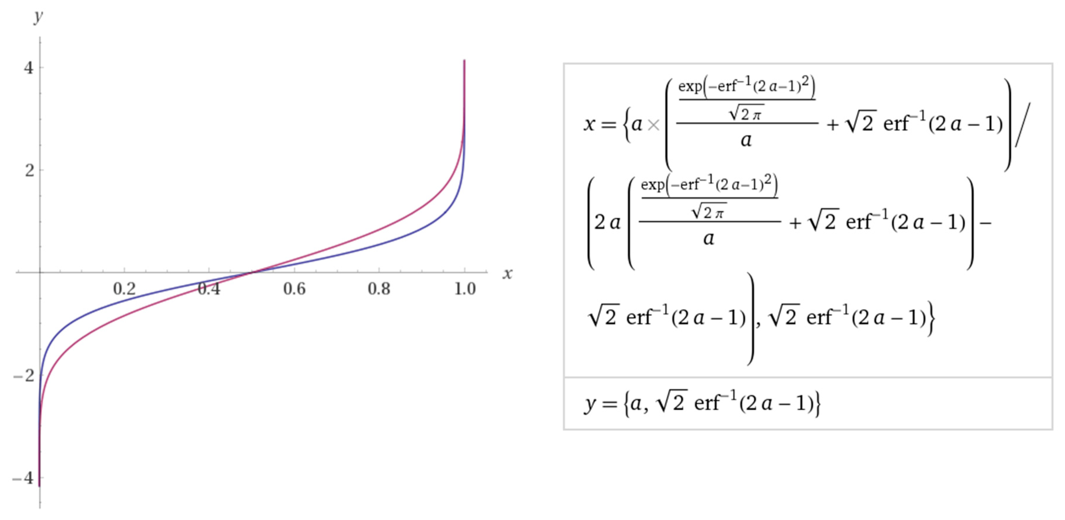
Figure 2.
The expectile and quantile functions for the uniform distribution, U(0, 1).

Figure 3.
Identical expectile and quantile functions for the Koenker distribution.

Figure 4.
The Koenker distribution as a scaled version of Student’s t distribution, ν = 2.


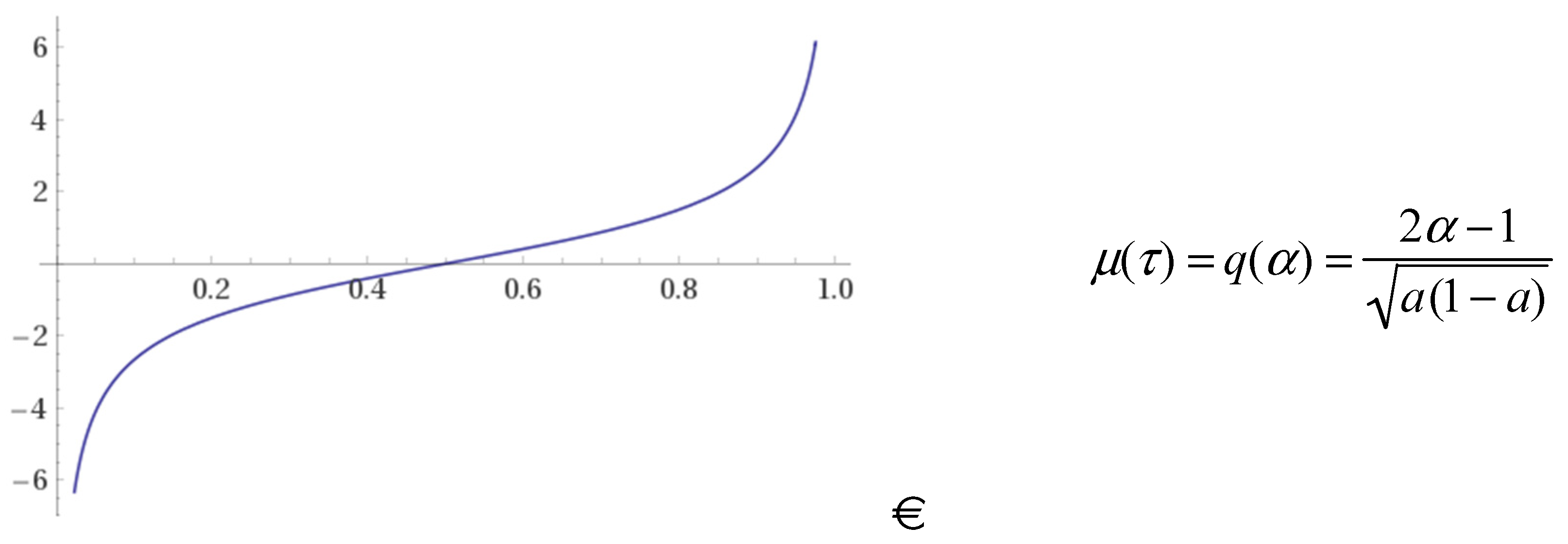
Table 1.
Multiplication factor 3 + k according to Basel’s traffic-light system.
| Zone | Exceedances | Plus Factor k | Cumulative Probability (in %) |
|---|---|---|---|
| ■ | 0 | 0.00 | 08.11 |
| ■ | 1 | 0.00 | 28.58 |
| ■ | 2 | 0.00 | 54.32 |
| ■ | 3 | 0.00 | 75.81 |
| ■ | 4 | 0.00 | 89.22 |
| ■ | 5 | 0.40 | 95.88 |
| ■ | 6 | 0.50 | 98.63 |
| ■ | 7 | 0.65 | 99.60 |
| ■ | 8 | 0.75 | 99.89 |
| ■ | 9 | 0.85 | 99.97 |
| ■ | 10+ | 1.00 | 99.99 |
Table 2.
Traffic light approaches to traditional and comparative backtesting.
| Zone | Traditional | Comparative |
|---|---|---|
| VaR (BCBS 2013): | Nolde and Ziegel (2017a): : The internal model predicts at least as well as the standard model. : The internal model predicts at most as well as the standard model. Some choice of significance level . E.g., = 0.05. | |
| Expected shortfall (Costanzino and Curran 2018): | ||
| ■ | is rejected at = 0.05. | |
| ■ | Neither nor is rejected | |
| ■ | is rejected at = 0.05. |
Table 3.
Normally distributed VaR, expected shortfall, and τ for different values of α.
| α | VaRα | ESα | τ(α) |
|---|---|---|---|
| 0.00135000 | –2.99998 | –3.28308 | 0.000127364 |
| 0.00353299 | –2.69372 | –3.00000 | 0.000401386 |
| 0.010000 | –2.32648 | –2.66521 | 0.00145241 |
| 0.025000 | –1.95996 | –2.33780 | 0.00477345 |
| 0.050000 | –1.64485 | –2.06271 | 0.0123873 |
© 2018 by the author. Licensee MDPI, Basel, Switzerland. This article is an open access article distributed under the terms and conditions of the Creative Commons Attribution (CC BY) license (http://creativecommons.org/licenses/by/4.0/).
Share and Cite
MDPI and ACS Style
Chen, J.M. On Exactitude in Financial Regulation: Value-at-Risk, Expected Shortfall, and Expectiles. Risks 2018, 6, 61. https://doi.org/10.3390/risks6020061
AMA Style
Chen JM. On Exactitude in Financial Regulation: Value-at-Risk, Expected Shortfall, and Expectiles. Risks. 2018; 6(2):61. https://doi.org/10.3390/risks6020061
Chicago/Turabian StyleChen, James Ming. 2018. "On Exactitude in Financial Regulation: Value-at-Risk, Expected Shortfall, and Expectiles" Risks 6, no. 2: 61. https://doi.org/10.3390/risks6020061
Note that from the first issue of 2016, this journal uses article numbers instead of page numbers. See further details here.