On the Moments and the Distribution of Aggregate Discounted Claims in a Markovian Environment

Abstract

This paper studies the moments and the distribution of the aggregate discounted claims (ADCs) in a Markovian environment, where the claim arrivals, claim amounts, and forces of interest (for discounting) are influenced by an underlying Markov process. Specifically, we assume that claims occur according to a Markovian arrival process (MAP). The paper shows that the vector of joint Laplace transforms of the ADC occurring in each state of the environment process by any specific time satisfies a matrix-form first-order partial differential equation, through which a recursive formula is derived for the moments of the ADC occurring in certain states (a subset). We also study two types of covariances of the ADC occurring in any two subsets of the state space and with two different time lengths. The distribution of the ADC occurring in certain states by any specific time is also investigated. Numerical results are also presented for a two-state Markov-modulated model case.

1. Introduction

Consider a line of business or an insurance portfolio to be insured by a property and casualty insurance company. Suppose that random claims arrive in the future according to a counting process, denoted by ${\left\{N\left(t\right)\right\}}_{t\ge 0}$, i.e., $N\left(t\right)$ is the random number of claims up to time t. Assume that ${\left\{T_n\right\}}_{n\ge 1}$ is a sequence of random claim occurrence times and ${\left\{X_n\right\}}_{n\ge 1}$ is a sequence of corresponding random positive claim amounts (also called claim severities), and $\delta \left(t\right)$ is the force of interest at time t, which is modeled by a stochastic process. Then $S\left(t\right)$ defined by

$$S\left(t\right)=\sum _{n=1}^{N\left(t\right)}{X}_n{e}^{-{\int }_0^{T_n}\delta \left(s\right)ds},t\ge 0$$

(1)

is the aggregate discounted claims (ADCs) up to certain time t, or the present value of the total amounts paid out by the company up to time t, which describes the random change over time of the insurer’s future liabilities at present time. Accordingly, ${\left\{S\left(t\right)\right\}}_{t\ge 0}$ is the ADC process (compound discounted claims) for this business. At a fixed time t, the randomness of $S\left(t\right)$ comes from the number of claims up to time t, claim occurrence times, and corresponding sizes as well as the values of $\delta \left(s\right),0\le s\le t$. It is an important quantity in the sense that, at the time of issue ($t=0$), this quantity would help insurers set a premium for this particular line of business, and predict and manage their future liabilities.

A simple case of model (1) is one in which the counting process ${\left\{N\left(t\right)\right\}}_{t\ge 0}$ is a homogeneous Poisson process, independent of claim amounts, and the force of interest is deterministic. In this paper, we assume that the counting process ${\left\{N\left(t\right)\right\}}_{t\ge 0}$ is a Markovian arrival process (MAP) with representation $(\gamma ,{\mathbf{D}}_{\mathbf{0}},{\mathbf{D}}_{\mathbf{1}})$, introduced by Neuts (1979). That is, claim arrivals are influenced by an underlying continuous-time Markov process ${\left\{J\left(t\right)\right\}}_{t\ge 0}$ on state space $E=\{1,2,\dots ,m\}$ with an $m\times m$ intensity matrix $\mathbf{D}$ and initial distribution $\gamma$, where $\mathbf{D}={\mathbf{D}}_{\mathbf{0}}+{\mathbf{D}}_{\mathbf{1}}=\left(d_{0,ij}\right)+\left(d_{1,ij}\right)$, and is assumed to be irreducible. Precisely, $d_{0,ij}$ represents the intensity of transitions from state i to state j without claim arrivals, while $d_{1,ij}(\ge 0)$ represents the intensity of transitions from state i to state j with an accompanying claim, having a cumulative distribution function $F_i$, density function $f_i,$ k-th moment ${\mu }_i^{\left(k\right)},$ and Laplace transform ${\widehat{f}}_i\left(s\right)={\int }_0^{\infty }{e}^{-sx}{f}_i\left(x\right)dx.$ Here, the process ${\left\{J\left(t\right)\right\}}_{t\ge 0}$ models the random environment, which affects the frequency and the severity of claims and thus the insurance business; for example, it is well known that the weather or climate conditions have impacts on automobile, property and casualty insurance claims.

Moreover, we assume that the force of interest process ${\left\{\delta \left(t\right)\right\}}_{t\ge 0}$ in (1) is also governed by the same Markov process ${\left\{J\left(t\right)\right\}}_{t\ge 0}$ and is assumed constant while staying at certain state, that is, when $J\left(t\right)=i,$ $\delta \left(t\right)={\delta }_i(>0)$, for all $i\in E$. As the force of interest used for evaluation is mainly driven by the local or global economics conditions, we would reasonably model its random fluctuations by a stochastic process that is different from ${\left\{J\left(t\right)\right\}}_{t\ge 0}$. Technically, we can assume a two-dimensional Markov process as the environment or background process and other mathematical treatments would be the same as we do below. Hence, we make the above assumption in this paper to simplify notations and presentations. We note that studies of the influence of economic conditions such as interest and inflation on the classical risk theory can be found in papers by Taylor (1979), Delbaen and Haezendonck (1987), Willmot (1989), and Garrido and Léveill (2004).

The MAP has received considerable attention in recent decades due to its versatility and feasibility in modeling stochastic insurance claims dynamics. MAPs include Poisson processes, renewal processes with the inter-arrival times following phase-type distributions, and Markov-modulated Poisson processes as special cases, which are intensively studied in actuarial science literature. Detailed characteristics and properties of MAPs can be found in papers by Neuts (1979) and Asmussen (2003). Below, we present a brief literature review on the related work based on models given by Equation (1) (including its special cases).

Most of the studies on model (1) are under the assumption that ${\left\{\delta \left(t\right)\right\}}_{t\ge 0}$ is deterministic. For the ADC, Léveillé and Garrido (2001a) give explicit expressions for its first two moments in the compound renewal risk process by using renewal theory arguments, while Léveillé and Garrido (2001b) further derive a recursive formula for the moments calculation. Léveillé et al. (2010) study the moment generating function (mgf) of the ADC by finite and infinite time under a renewal risk model or a delayed renewal risk model. Recently, Wang et al. (2018) studied the distribution of discounted compound phase-type renewal sums using the analytical results of their mgf obtained by Léveillé et al. (2010). Jang (2004) obtains the Laplace transform of the distribution of the ADC using a shot noise process. Woo and Cheung (2013) derive recursive formulas for the moments of the ADC using techniques used by Léveillé and Garrido (2001b), for a renewal risk process with certain dependence between the claim arrival and the amount caused. The impact of the dependency on the ADC are illustrated numerically. Kim and Kim (2007) derive simple expressions for the first two moments of the ADC when the rates of claim arrivals and the claim sizes depend on the states of an underlying Markov process. Ren (2008) studies the Laplace transform and the first two moments of the ADC following a MAP process, and Li (2008) further derives a recursive formula for the moments of the discounted claims for the same model. Barges et al. (2011) study the moments of the ADC in a compound Poisson model with dependence introduced by a Farlie–Gumbel–Morgenstern (FGM) copula; Mohd Ramli and Jang (2014) further derive Neumann series expression of the recursive moments by using the method of successive approximation.

There are few papers that study models described by Equation (1) with a stochastic process ${\left\{\delta \left(t\right)\right\}}_{t\ge 0}$ in the literature of actuarial science. Leveille and Adekambi (2011, 2012) study the covariance and the joint moments of the discounted compound renewal sum at two different times with a stochastic interest rate where the Ho–Lee–Merton and the Vasicek interest rate models are considered. Their idea of studying the covariance and the joint moments is adopted and extended in this paper. Here, we assume that the components of the ADC process ${\left\{S\left(t\right)\right\}}_{t\ge 0}$ described by Equation (1)—the number of claims, the size of the claims, and the force of interest for discounting—are all influenced by the same Markovian environment process, which enhances the flexibility of the model parameter settings. It follows that $S\left(t\right)$ depends on the trajectory of this underlying process whose states may represent different external conditions or circumstances that affect insurance claims. The main objective of this paper is to study the moments and the distribution of $S\left(t\right)$ given in Equation (1), occurring in certain states (e.g., certain conditions) by time t.

In general, while the expectation of $S\left(t\right)$ at any given time t can be used as a reference for the insurer’s liability, the higher moments of $S\left(t\right)$, describing further characteristics of the random variable such as the variability around the mean and how extreme outcomes could go, may be used to determine the marginals on reserves. Furthermore, the distributional results regarding $S\left(t\right)$ would be useful for obtaining the risk measures such as the value at risk and the conditional tail expectation, which may help insurers prevent or minimize their losses from extreme cases.

Our work is basically a generalization of some aforementioned studies. We first obtain formulas for calculating mean, variance, and distribution of the ADC occurring in a subset of states at a certain time. The subset may represent a collection of similar conditions that the insurer would consider them as a whole. We then derive explicit matrix-analytic expressions for covariances of the ADC occurring in two subsets of the state space at a certain time and those occurring in a certain subset of states with two different time lengths. The motivation of studying these two types of covariance is that we believe they can reveal the correlation between the random discounted sums either between different underlying conditions or with different time lengths, and the information would be helpful for insurers to set their capital requirements for preventing future losses, and make strategic and contingency plans. Moreover, we obtain a matrix-form partial integro-differential equation satisfied by the distribution function of the ADC occurring in certain subset of states. The equation can be solved numerically to obtain the probability distribution function of the ADC, which again could be useful for measuring insurers’ risks of insolvency.

The rest of the paper is organized as follows. In Section 2, we study the joint Laplace transforms of the ADC occurring in each state by time t and pay attention to some special cases. Recursive formulas for calculating the moments of the ADC occurring in certain states are obtained. A formula for computing the covariance of the ADC occurring in two subsets of the state space is derived in Section 3, while the covariance of the ADC occurring in certain states with two different time lengths is studied in Section 4. The distribution of the ADC occurring in certain states is investigated in Section 5. Finally, some numerical illustrations are presented in Section 6.

2. The Laplace Transforms and Moments

We first decompose $S\left(t\right)$ into m components as

$$S\left(t\right)=\sum _{j=1}^m{S}_j\left(t\right)$$

where

$$S_j\left(t\right)=\sum _{n=1}^{N\left(t\right)}{X}_{n}I(J\left(T_n\right)=j)e^{-{\int }_0^{T_n}\delta \left(s\right)ds}$$

is the ADC occurring in state $j\in E,$ with $I(·)$ being the indicator function. For a given $k(1\le k\le m$), $1\le l_1<l_2<\dots <l_k\le m$ denote $E_k=\{l_1,l_2,\dots ,l_k\}\subseteq E,$ a sub-state space of E. We then define

$$S_{E_k}\left(t\right)=\sum _{j\in E_k}{S}_j\left(t\right)$$

to be the ADC occurring in the subset of state space $E_k.$ In particular, $S_E\left(t\right)=S\left(t\right)$ and $S_{\left\{j\right\}}\left(t\right)=S_j\left(t\right).$ If $\delta \left(t\right)=0$ and $X_i\equiv 1$ for all $i\in {\mathbb{N}}^{+}$, then $S_{E_k}\left(t\right)=N_{E_k}\left(t\right)$, where $N_{E_k}\left(t\right)$ is the number of claims occurring in the sub-state space $E_k$ by time t.

Let ${\mathbb{P}}_i$ and ${\mathbb{E}}_i$ denote conditional probability and conditional expectation given $J\left(0\right)=i$, respectively. Define

$${}_{i}L({\xi }_1,{\xi }_2,\dots ,{\xi }_m;t)={\mathbb{E}}_i\left[e^{-{\sum }_{j=1}^m{\xi }_j{S}_j\left(t\right)}\right],{\xi }_j\ge 0,t\ge 0,i\in E$$

(2)

to be the joint Laplace transform of $S_1\left(t\right),S_2\left(t\right),\dots ,S_m\left(t\right),$ given that the initial state is $i.$ In particular, we have

$$\begin{array}{cc}\hfill {}_{i}L(\xi ;t)& ={\mathbb{E}}_i\left[e^{-\xi S\left(t\right)}\right]={}_{i}L(\xi ,\xi ,\dots ,\xi ;t)\hfill \\ \hfill {}_i{L}_{E_k}(\xi ;t)& ={\mathbb{E}}_i\left[e^{-\xi S_{E_k}\left(t\right)}\right]={}_{i}L({\xi }_1,{\xi }_2,\dots ,{\xi }_m;t){|}_{{\xi }_j=\xi I(j=l_n),n=1,2,\dots ,k}\hfill \\ \hfill {}_i{L}_j({\xi }_j;t)& ={\mathbb{E}}_i\left[e^{-{\xi }_j{S}_j\left(t\right)}\right]={}_{i}L({\xi }_1,{\xi }_2,\dots ,{\xi }_m;t){|}_{{\xi }_k=0,k\ne j}.\hfill \end{array}$$

We define, for $n\in {\mathbb{N}}^{+},$ the n-th moment of $S\left(t\right)$, $S_j\left(t\right)$, and $S_{E_k}\left(t\right)$, respectively, as

$$\begin{array}{cc}\hfill {}_i{V}^{\left(n\right)}\left(t\right)& ={\mathbb{E}}_i\left[S^n\left(t\right)\right],i\in E\hfill \\ \hfill {}_i{V}_j^{\left(n\right)}\left(t\right)& ={\mathbb{E}}_i\left[S_j^n\left(t\right)\right],i,j\in E\hfill \\ \hfill {}_i{V}_{E_k}^{\left(n\right)}\left(t\right)& ={\mathbb{E}}_i\left[S_{E_k}^n\left(t\right)\right],1\le k\le m\hfill \end{array}$$

given that the initial state is i.

We write the following column vectors for the Laplace transforms

$$\begin{array}{cc}\hfill \mathbf{L}({\xi }_1,{\xi }_2,\dots ,{\xi }_m;t)& ={\left({}_{1}L({\xi }_1,{\xi }_2,\dots ,{\xi }_m;t),\dots ,{}_{m}L({\xi }_1,{\xi }_2,\dots ,{\xi }_m;t)\right)}^{\top }\hfill \\ \hfill \mathbf{L}(\xi ;t)& ={\left({}_{1}L(\xi ;t),{}_{2}L(\xi ;t),\dots ,{}_{m}L(\xi ;t)\right)}^{\top }\hfill \\ \hfill {\mathbf{L}}_{E_k}(\xi ;t)& ={\left({}_1{L}_{E_k}(\xi ;t),{}_2{L}_{E_k}(\xi ;t),\dots ,{}_m{L}_{E_k}(\xi ;t)\right)}^{\top }\hfill \\ \hfill {\mathbf{L}}_j({\xi }_j;t)& ={\left({}_1{L}_j({\xi }_j;t),{}_2{L}_j({\xi }_j;t),\dots ,{}_m{L}_j({\xi }_j;t)\right)}^{\top },\hfill \end{array}$$

with $\mathbf{L}(0;t)={\mathbf{L}}_{E_k}(0;t)={\mathbf{L}}_j(0;t)=\mathbf{1}={(1,1,\dots ,1)}^{\top }.$

In this section, we first show that $\mathbf{L}({\xi }_1,{\xi }_2,\dots ,{\xi }_m;t)$ satisfies a matrix-form first-order partial differential equation, and derive recursive formulas for calculating the moments of various ADC depending on the initial state of the underlying Markovian process. We also consider some special cases.

Theorem 1.

$\mathbf{L}({\xi }_1,{\xi }_2,\dots ,{\xi }_m;t)$ satisfies

$$\begin{array}{c}\frac{\partial \mathbf{L}({\xi }_1,{\xi }_2,\dots ,{\xi }_m;t)}{\partial t}+\delta \sum _{j=1}^m{\xi }_j\frac{\partial \mathbf{L}({\xi }_1,{\xi }_2,\dots ,{\xi }_m;t)}{\partial {\xi }_j}\hfill \\ ={\mathbf{D}}_0\mathbf{L}({\xi }_1,{\xi }_2,\dots ,{\xi }_m;t)+\widehat{\mathbf{f}}({\xi }_1,{\xi }_2,\dots ,{\xi }_m){\mathbf{D}}_1\mathbf{L}({\xi }_1,{\xi }_2,\dots ,{\xi }_m;t)\hfill \end{array}$$

(3)

where $\delta =\mathit{diag}({\delta }_1,{\delta }_2,\dots ,{\delta }_m)$ and $\widehat{\mathbf{f}}({\xi }_1,{\xi }_2,\dots ,{\xi }_m)=\mathit{diag}({\widehat{f}}_1\left({\xi }_1\right),{\widehat{f}}_2\left({\xi }_2\right),\dots ,{\widehat{f}}_m\left({\xi }_m\right)).$

Proof. 

For an infinitesimal $h>0$, conditioning on three possible events which can occur in $[0,h]$—no change in the MAP phase (state), a change in the MAP phase accompanied by no claims, and a change in the MAP phase accompanied by a claim—we have

$$\begin{array}{cc}\hfill {}_{i}L({\xi }_1,{\xi }_2,\dots ,{\xi }_m;t)=& [1+d_{0,ii}h]{}_{i}L\left({\xi }_1{e}^{-{\delta }_{i}h},{\xi }_2{e}^{-{\delta }_{i}h},\dots ,{\xi }_m{e}^{-{\delta }_{i}h};t-h\right)\hfill \\ & +\sum _{k=1,k\ne i}^m{d}_{0,ik}h{}_{k}L\left({\xi }_1{e}^{-{\delta }_{i}h},{\xi }_2{e}^{-{\delta }_{i}h},\dots ,{\xi }_m{e}^{-{\delta }_{i}h};t-h\right)\hfill \\ & +\sum _{k=1}^m{d}_{1,ik}h{\widehat{f}}_i\left({\xi }_i{e}^{-{\delta }_{i}h}\right){}_{k}L\left({\xi }_1{e}^{-{\delta }_{i}h},{\xi }_2{e}^{-{\delta }_{i}h},\dots ,{\xi }_m{e}^{-{\delta }_{i}h};t-h\right).\hfill \end{array}$$

(4)

As ${}_{i}L({\xi }_1,{\xi }_2,\dots ,{\xi }_m;t)$ is differentiable with respect to ${\xi }_i(i\in E)$ and t (the differentiability of ${}_{i}L$ with respect to t is justified in Appendix), we have

$$\begin{array}{c}{}_{i}L\left({\xi }_1{e}^{-{\delta }_{i}h},{\xi }_2{e}^{-{\delta }_{i}h},\dots ,{\xi }_m{e}^{-{\delta }_{i}h};t-h\right)\hfill \\ ={}_{i}L({\xi }_1,{\xi }_2,\dots ,{\xi }_m;t)-h\frac{\partial {}_{i}L({\xi }_1,{\xi }_2,\dots ,{\xi }_m;t)}{\partial t}-{\delta }_{i}h\sum _{l=1}^m{\xi }_l\frac{\partial {}_{i}L({\xi }_1,{\xi }_2,\dots ,{\xi }_m;t)}{\partial {\xi }_l}+o\left(h\right)\hfill \end{array}$$

(5)

where ${lim}_{h\to 0}(o\left(h\right)/h)=0$. Substituting the expression above into Equation (4), dividing both sides by h, and letting $h\to 0,$ we have

$$\begin{array}{c}{\delta }_i\sum _{l=1}^m{\xi }_l\frac{\partial {}_{i}L({\xi }_1,{\xi }_2,\dots ,{\xi }_m;t)}{\partial {\xi }_l}+\frac{\partial {}_{i}L({\xi }_1,{\xi }_2,\dots ,{\xi }_m;t)}{\partial t}\hfill \\ =\sum _{k=1}^m{d}_{0,ik}{}_{k}L({\xi }_1,{\xi }_2,\dots ,{\xi }_m;t)+\sum _{k=1}^m{d}_{1,ik}{\widehat{f}}_i\left({\xi }_i\right){}_{k}L({\xi }_1,{\xi }_2,\dots ,{\xi }_m;t).\hfill \end{array}$$

(6)

Rewriting Equation (6) in matrix form gives Equation (3). ☐

Remark 1.

Using the same argument, we have the follow results.

(1) 

${\mathbf{L}}_{E_k}(\xi ;t)$ satisfies the following matrix-form first-order partial differential equation:

$$\begin{array}{c}\hfill \frac{\partial {\mathbf{L}}_{E_k}(\xi ;t)}{\partial t}+\delta \xi \frac{\partial {\mathbf{L}}_{E_k}(\xi ;t)}{\partial \xi }={\mathbf{D}}_0{\mathbf{L}}_{E_k}(\xi ;t)+{\widehat{\mathbf{f}}}_{E_k}\left(\xi \right){\mathbf{D}}_{\mathbf{1}}{\mathbf{L}}_{E_k}(\xi ;t)\end{array}$$

(7)

where ${\widehat{\mathbf{f}}}_{E_k}\left(\xi \right)$ is an $m\times m$ diagonal matrix with the $l_i$-th entry being ${\widehat{f}}_{l_i}\left(\xi \right)$, for $i=1,2,\dots ,k$ and all other entries being 1.

(2) 

$\mathbf{L}(\xi ;t)$ satisfies

$$\begin{array}{c}\hfill \frac{\partial \mathbf{L}(\xi ;t)}{\partial t}+\delta \xi \frac{\partial \mathbf{L}(\xi ;t)}{\partial \xi }={\mathbf{D}}_0\mathbf{L}(\xi ;t)+\widehat{\mathbf{f}}\left(\xi \right){\mathbf{D}}_{\mathbf{1}}\mathbf{L}(\xi ;t)\end{array}$$

where $\widehat{\mathbf{f}}\left(\xi \right)=\mathit{diag}({\widehat{f}}_1\left(\xi \right),{\widehat{f}}_2\left(\xi \right),\dots ,{\widehat{f}}_m\left(\xi \right)).$

(3) 

${\mathbf{L}}_j({\xi }_j;t)$ satisfies

$$\begin{array}{c}\hfill \frac{\partial {\mathbf{L}}_j({\xi }_j;t)}{\partial t}+\delta {\xi }_j\frac{\partial {\mathbf{L}}_j({\xi }_j;t)}{\partial {\xi }_j}={\mathbf{D}}_0{\mathbf{L}}_j({\xi }_j;t)+{\widehat{\mathbf{f}}}_j\left({\xi }_j\right){\mathbf{D}}_1{\mathbf{L}}_j({\xi }_j;t)\end{array}$$

where ${\widehat{\mathbf{f}}}_j\left({\xi }_j\right)=\mathit{diag}(1,1,\dots ,{\widehat{f}}_j\left({\xi }_j\right),1,\dots ,1).$

We now study the moments of the ADC considered in Theorem 1. Denote the vectors of the n-th moment of the corresponding ADC as

$$\begin{array}{cc}\hfill {\mathbf{V}}_n\left(t\right)& ={({}_1{V}^{\left(n\right)}\left(t\right),{}_2{V}^{\left(n\right)}\left(t\right),\dots ,{}_m{V}^{\left(n\right)}\left(t\right))}^{\top }\hfill \\ \hfill {\mathbf{V}}_{n,E_k}\left(t\right)& ={({}_1{V}_{E_k}^{\left(n\right)}\left(t\right),{}_2{V}_{E_k}^{\left(n\right)}\left(t\right),\dots ,{}_m{V}_{E_k}^{\left(n\right)}\left(t\right))}^{\top }\hfill \\ \hfill {\mathbf{V}}_{n,j}\left(t\right)& ={({}_1{V}_j^{\left(n\right)}\left(t\right),{}_2{V}_j^{\left(n\right)}\left(t\right),\dots ,{}_m{V}_j^{\left(n\right)}\left(t\right))}^{\top }.\hfill \end{array}$$

From Equation (7), we obtain in Theorem 2 a matrix-form first-order differential equation satisfied by the moments of $S_{E_k}\left(t\right),$ ${\mathbf{V}}_{n,E_k}\left(t\right)$ and then, in Theorem 3, obtain recursive formulas for calculating them.

Theorem 2.

The moments of $S_{E_k}\left(t\right)$ satisfy

$$\begin{array}{c}\hfill {\mathbf{V}}_{n,E_k}^{\prime }\left(t\right)+\left(n\delta -{\mathbf{D}}_0-{\mathbf{D}}_1\right){\mathbf{V}}_{n,E_k}\left(t\right)=\sum _{r=1}^n\left(\genfrac{}{}{0pt}{}{n}{r}\right){\mathbf{I}}_{E_k}{\mu }_r{\mathbf{D}}_1{\mathbf{V}}_{n-r,E_k}\left(t\right),n\in {\mathbb{N}}^{+},\end{array}$$

(8)

with initial conditions ${\mathbf{V}}_{n,E_k}\left(0\right)=\mathbf{0}$ and ${\mathbf{V}}_{0,E_k}\left(t\right)=\mathbf{1}.$ In particular,

$$\begin{array}{c}\hfill {\mathbf{V}}_{1,E_k}^{\prime }\left(t\right)+\left(\delta -{\mathbf{D}}_0-{\mathbf{D}}_1\right){\mathbf{V}}_{1,E_k}\left(t\right)={\mathbf{I}}_{E_k}{\mu }_1{\mathbf{D}}_1\mathbf{1},t\ge 0\end{array}$$

where ${\mu }_r=\mathit{diag}({\mu }_1^{\left(r\right)},{\mu }_2^{\left(r\right)},\dots ,{\mu }_m^{\left(r\right)})$, ${\mathbf{I}}_{E_k}$ is an $m\times m$ diagonal matrix with the $l_i$-th entry being $1,$ for $i=1,2,\dots ,k,$ and all other diagonal entries being $0.$

Proof. 

By Taylor’s expansion (its existence is easily justified as we assume that $f_i$ has moment ${\mu }_i^{\left(n\right)}$ for any $n\in {\mathbb{N}}^{+}$), we have

$${\widehat{f}}_i\left(\xi \right)=1+\sum _{n=1}^{\infty }\frac{{(-1)}^n{\xi }^n}{n!}{\mu }_i^{\left(n\right)}.$$

In matrix notation,

$${\widehat{\mathbf{f}}}_{E_k}\left(\xi \right)=\mathbf{1}+\sum _{n=1}^{\infty }\frac{{(-1)}^n{\xi }^n}{n!}{\mathbf{I}}_{E_k}{\mathbf{\mu }}_n.$$

(9)

Substituting Equation (9) together with

$${\mathbf{L}}_{E_k}(\xi ;t)=\sum _{n=0}^{\infty }\frac{{(-1)}^n{\xi }^n}{n!}{\mathbf{V}}_{n,E_k}\left(t\right)$$

into Equation (7) and equating the coefficients of ${\xi }^n$ give Equation (8). ☐

Corollary 1.

We have the following results for the moments of $S\left(t\right)$ and $S_j\left(t\right).$

(i) 

${\mathbf{V}}_n\left(t\right)$ satisfies the matrix-form first-order differential equation:

$${\mathbf{V}}_n^{\prime }\left(t\right)+\left(n\delta -{\mathbf{D}}_0-{\mathbf{D}}_1\right){\mathbf{V}}_n\left(t\right)=\sum _{r=1}^n\left(\genfrac{}{}{0pt}{}{n}{r}\right){\mathbf{\mu }}_r{\mathbf{D}}_1{\mathbf{V}}_{n-r}\left(t\right),n\in {\mathbb{N}}^{+}$$

where ${\mathbf{V}}_n\left(0\right)=\mathbf{0}$ and ${\mathbf{V}}_0\left(t\right)=\mathbf{1}.$ In particular, ${\mathbf{V}}_1\left(t\right)$ satisfies

$$\begin{array}{c}\hfill {\mathbf{V}}_1^{\prime }\left(t\right)+\left(\delta -{\mathbf{D}}_0-{\mathbf{D}}_1\right){\mathbf{V}}_1\left(t\right)={\mathbf{\mu }}_1{\mathbf{D}}_1\mathbf{1},t\ge 0.\end{array}$$

(ii) 

${\mathbf{V}}_{n,j}\left(t\right)$ satisfies

$$\begin{array}{c}\hfill {\mathbf{V}}_{n,j}^{\prime }\left(t\right)+\left(n\delta -{\mathbf{D}}_0-{\mathbf{D}}_1\right){\mathbf{V}}_{n,j}\left(t\right)=\sum _{r=1}^n\left(\genfrac{}{}{0pt}{}{n}{r}\right){\mathbf{I}}_j{\mathbf{\mu }}_r{\mathbf{D}}_1{\mathbf{V}}_{n-r,j}\left(t\right)\end{array}$$

where ${\mathbf{I}}_j={\mathbf{I}}_{\left\{j\right\}}$ is a diagonal matrix with the j-th entry being $1,$ and 0 otherwise, ${\mathbf{V}}_{n,j}\left(0\right)=\mathbf{0}$ and ${\mathbf{V}}_{0,j}\left(t\right)=\mathbf{1}.$ In particular, ${\mathbf{V}}_{1,j}\left(t\right)$ satisfies

$$\begin{array}{c}\hfill {\mathbf{V}}_{1,j}^{\prime }\left(t\right)+\left(\delta -{\mathbf{D}}_0-{\mathbf{D}}_1\right){\mathbf{V}}_{1,j}\left(t\right)={\mathbf{I}}_j{\mu }_1{\mathbf{D}}_1\mathbf{1},t\ge 0.\end{array}$$

Solving differential Equation (8) with ${\mathbf{V}}_{n,E_k}\left(0\right)=\mathbf{0}$, we obtain the following recursive formulas for ${\mathbf{V}}_{n,E_k}\left(t\right)$.

Theorem 3.

For $t>0$ and $n\in {\mathbb{N}}^{+},$ we have

$$\begin{array}{c}\hfill {\mathbf{V}}_{n,E_k}\left(t\right)=\sum _{r=1}^n\left(\genfrac{}{}{0pt}{}{n}{r}\right){\int }_0^t{e}^{-\left(n\delta -({\mathbf{D}}_0+{\mathbf{D}}_{\mathbf{1}})\right)x}{\mathbf{I}}_{E_k}{\mathbf{\mu }}_r{\mathbf{D}}_1{\mathbf{V}}_{n-r,E_k}(t-x)dx.\end{array}$$

In particular,

$$\begin{array}{cc}\hfill {\mathbf{V}}_{1,E_k}\left(t\right)& ={\int }_0^t{e}^{-\left(\delta -({\mathbf{D}}_0+{\mathbf{D}}_{\mathbf{1}})\right)x}dx{\mathbf{I}}_{E_k}{\mathbf{\mu }}_1{\mathbf{D}}_1\mathbf{1}\hfill \\ & ={[\delta -({\mathbf{D}}_0+{\mathbf{D}}_{\mathbf{1}})]}^{-1}\left[\mathbf{I}-e^{-[\delta -({\mathbf{D}}_0+{\mathbf{D}}_{\mathbf{1}})]t}\right]{\mathbf{I}}_{E_k}{\mathbf{\mu }}_1{\mathbf{D}}_1\mathbf{1}.\hfill \end{array}$$

(10)

Clearly, we have ${\mathbf{V}}_{1,E_k}\left(t\right)+{\mathbf{V}}_{1,E_k^c}\left(t\right)={\mathbf{V}}_1\left(t\right),$ where $E_k^c=E\backslash E_k$.

Corollary 2.

If we set $E_k=E$ and $E_k=\left\{j\right\}$ in Theorem 3, we have the following recursive formulas for the moments of $S\left(t\right)$ and $S_j\left(t\right)$:

$$\begin{array}{cc}\hfill {\mathbf{V}}_n\left(t\right)& =\sum _{k=1}^n\left(\genfrac{}{}{0pt}{}{n}{k}\right){\int }_0^t{e}^{-\left(n\delta -({\mathbf{D}}_0+{\mathbf{D}}_{\mathbf{1}})\right)x}{\mathbf{\mu }}_k{\mathbf{D}}_1{\mathbf{V}}_{n-k}(t-x)dx\hfill \\ \hfill {\mathbf{V}}_{n,j}\left(t\right)& =\sum _{k=1}^n\left(\genfrac{}{}{0pt}{}{n}{k}\right){\int }_0^t{e}^{-\left(n\delta -({\mathbf{D}}_0+{\mathbf{D}}_{\mathbf{1}})\right)x}{\mathbf{I}}_j{\mathbf{\mu }}_k{\mathbf{D}}_1{\mathbf{V}}_{n-k,j}(t-x)dx.\hfill \end{array}$$

In particular,

$$\begin{array}{cc}\hfill {\mathbf{V}}_1\left(t\right)& ={[\delta -({\mathbf{D}}_0+{\mathbf{D}}_{\mathbf{1}})]}^{-1}\left[\mathbf{I}-e^{-[\delta -({\mathbf{D}}_0+{\mathbf{D}}_{\mathbf{1}})]t}\right]{\mathbf{\mu }}_1{\mathbf{D}}_1\mathbf{1}\hfill \\ \hfill {\mathbf{V}}_{1,j}\left(t\right)& ={[\delta -({\mathbf{D}}_0+{\mathbf{D}}_{\mathbf{1}})]}^{-1}\left[\mathbf{I}-e^{-[\delta -({\mathbf{D}}_0+{\mathbf{D}}_{\mathbf{1}})]t}\right]{\mathbf{I}}_j{\mathbf{\mu }}_1{\mathbf{D}}_1\mathbf{1}.\hfill \end{array}$$

Remark 2.

When $t\to \infty$, we have the following asymptotic results for the moments of the ADC for $n\in {\mathbb{N}}^{+}$:

$$\begin{array}{cc}\hfill {\mathbf{V}}_{n,E_k}(\infty )& ={[n\delta -({\mathbf{D}}_0+{\mathbf{D}}_{\mathbf{1}})]}^{-1}\sum _{r=1}^n\left(\genfrac{}{}{0pt}{}{n}{r}\right){\mathbf{I}}_{E_k}{\mathbf{\mu }}_r{\mathbf{D}}_1{\mathbf{V}}_{n-r,E_k}(\infty )\hfill \\ \hfill {\mathbf{V}}_n(\infty )& ={[n\delta -({\mathbf{D}}_0+{\mathbf{D}}_{\mathbf{1}})]}^{-1}\sum _{r=1}^n\left(\genfrac{}{}{0pt}{}{n}{r}\right){\mathbf{\mu }}_r{\mathbf{D}}_1{\mathbf{V}}_{n-r}(\infty )\hfill \\ \hfill {\mathbf{V}}_{n,j}(\infty )& ={[n\delta -({\mathbf{D}}_0+{\mathbf{D}}_{\mathbf{1}})]}^{-1}\sum _{r=1}^n\left(\genfrac{}{}{0pt}{}{n}{r}\right){\mathbf{I}}_j{\mathbf{\mu }}_r{\mathbf{D}}_1{\mathbf{V}}_{n-r,j}(\infty )\hfill \end{array}$$

where ${\mathbf{V}}_{0,E_k}(\infty )={\mathbf{V}}_0(\infty )={\mathbf{V}}_{0,j}(\infty )=\mathbf{1}.$

3. The Covariance of ADC Occurring in Two Sub-State Spaces

In this section, we first calculate the joint moment of the ADC occurring in two subsets of the state space and then the covariance between them could be calculated.

For $1\le l_1<l_2<\dots <l_k\le m$ and $1\le n_1<n_2<\dots <n_j\le m$, where $2\le k+j\le m,$ denote $E_k=\{l_1,l_2,\dots ,l_k\}$ and $E_j=\{n_1,n_2,\dots ,n_j\}$ to be two disjoint subsets of E, i.e., $E_k\cap E_j=\varnothing .$ The aggregate discounted claim amounts occurring in $E_k$ and $E_j$ are

$$S_{E_k}\left(t\right)=\sum _{i\in E_k}{S}_i\left(t\right),S_{E_j}\left(t\right)=\sum _{i\in E_j}{S}_i\left(t\right).$$

Define

$${}_i{L}_{E_k,E_j}({\xi }_k,{\xi }_j;t)={\mathbb{E}}_i\left[e^{-{\xi }_k{S}_{E_k}\left(t\right)-{\xi }_j{S}_{E_j}\left(t\right)}\right]$$

to be the joint Laplace transform of $S_{E_k}\left(t\right)$ and $S_{E_j}\left(t\right)$. Let ${\mathbf{L}}_{E_k,E_j}({\xi }_k,{\xi }_j;t)$ be a column vector with the i-th entry being ${}_i{L}_{E_k,E_j}({\xi }_k,{\xi }_j;t).$ Moreover, let

$${}_i{V}_{E_k,E_j}\left(t\right)={\mathbb{E}}_i\left[S_{E_k}\left(t\right)S_{E_j}\left(t\right)\right]$$

be the joint moment of $S_{E_k}\left(t\right)$ and $S_{E_j}\left(t\right)$. Denote ${\mathbf{V}}_{E_k,E_j}\left(t\right)$ as an $m\times 1$ column vector with the i-th entry being ${}_i{V}_{E_k,E_j}\left(t\right)$. A matrix-form integral expression of ${\mathbf{V}}_{E_k,E_j}\left(t\right)$ and its asymptotic formula when $t\to \infty$ are presented in the theorem below.

Theorem 4.

For two disjoint subsets of E, $E_k$ and $E_j$, the joint moment of $S_{E_k}\left(t\right)$ and $S_{E_j}\left(t\right)$ satisfies

$$\begin{array}{cc}\hfill {\mathbf{V}}_{E_k,E_j}\left(t\right)=& {\int }_0^t{e}^{-\left(2\delta -({\mathbf{D}}_0+{\mathbf{D}}_1)\right)x}{\mathbf{I}}_{E_k}{\mathbf{\mu }}_1{\mathbf{D}}_{\mathbf{1}}{\mathbf{V}}_{1,E_j}(t-x)dx\hfill \\ & +{\int }_0^t{e}^{-\left(2\delta -({\mathbf{D}}_0+{\mathbf{D}}_1)\right)x}{\mathbf{I}}_{E_j}{\mathbf{\mu }}_1{\mathbf{D}}_{\mathbf{1}}{\mathbf{V}}_{1,E_k}(t-x)dx\hfill \end{array}$$

(11)

where ${\mathbf{V}}_{1,E_k}\left(t\right)$ is given by Equation (10) in Theorem 3. When $t\to \infty$, we have

$$\begin{array}{c}\hfill {\mathbf{V}}_{E_k,E_j}(\infty )={\left[2\delta -({\mathbf{D}}_0+{\mathbf{D}}_1)\right]}^{-1}\left[{\mathbf{I}}_{E_k}{\mathbf{\mu }}_1{\mathbf{D}}_{\mathbf{1}}{\mathbf{V}}_{1,E_j}(\infty )+{\mathbf{I}}_{E_j}{\mathbf{\mu }}_1{\mathbf{D}}_{\mathbf{1}}{\mathbf{V}}_{1,E_k}(\infty )\right].\end{array}$$

(12)

Proof. 

Following from Equation (3), we have

$$\begin{array}{c}\frac{\partial {\mathbf{L}}_{E_k,E_j}({\xi }_k,{\xi }_j;t)}{\partial t}+\delta {\xi }_k\frac{\partial {\mathbf{L}}_{E_k,E_j}({\xi }_k,{\xi }_j;t)}{\partial {\xi }_k}+\delta {\xi }_j\frac{\partial {\mathbf{L}}_{E_k,E_j}({\xi }_k,{\xi }_j;t)}{\partial {\xi }_j}\hfill \\ ={\mathbf{D}}_0{\mathbf{L}}_{E_k,E_j}({\xi }_k,{\xi }_j;t)+{\widehat{\mathbf{f}}}_{E_k,E_j}({\xi }_k,{\xi }_j){\mathbf{D}}_1{\mathbf{L}}_{E_k,E_j}({\xi }_k,{\xi }_j;t)\hfill \end{array}$$

(13)

where ${\widehat{\mathbf{f}}}_{E_k,E_j}({\xi }_k,{\xi }_j)$ is a diagonal matrix with the $l_i$-th entry being ${\widehat{f}}_{l_i}\left({\xi }_k\right)$, for $i=1,2,\dots ,k,$ with the $n_i$-th entry being ${\widehat{f}}_{n_i}\left({\xi }_j\right)$, for $i=1,2,\dots ,j,$ and all other elements being 1.

Taking partial derivatives with respect to ${\xi }_k$ and ${\xi }_j$ on both sides of Equation (13), setting ${\xi }_k=0$ and ${\xi }_j=0$, and noting that

$${}_i{V}_{E_k,E_j}\left(t\right)=\frac{{\partial }^2{}_i{L}_{E_k,E_j}({\xi }_k,{\xi }_j;t)}{\partial {\xi }_k\partial {\xi }_j}{|}_{{\xi }_k={\xi }_j=0},$$

we obtain the following matrix-form first-order differential equation for ${\mathbf{V}}_{E_k,E_j}\left(t\right)$:

$$\begin{array}{c}\hfill {\mathbf{V}}_{E_k,E_j}^{\prime }\left(t\right)+\left[2\delta -{\mathbf{D}}_0-{\mathbf{D}}_1\right]{\mathbf{V}}_{E_k,E_j}\left(t\right)={\mathbf{I}}_{E_k}{\mathbf{\mu }}_1{\mathbf{D}}_{\mathbf{1}}{\mathbf{V}}_{1,E_j}\left(t\right)+{\mathbf{I}}_{E_j}{\mathbf{\mu }}_1{\mathbf{D}}_{\mathbf{1}}{\mathbf{V}}_{1,E_k}\left(t\right).\end{array}$$

Solving it gives Equation (11).

Letting $t\to \infty$ in Equation (11), we obtain expression (12) for the joint moment of $S_{E_k}(\infty )$ and $S_{E_j}(\infty )$. ☐

Remark 3.

If $E_k=\left\{k\right\}$ and $E_j=\left\{j\right\},$ and $k\ne j,$ we have

$$\begin{array}{cc}\hfill {\mathbf{V}}_{\left\{k\right\},\left\{j\right\}}\left(t\right)=& {\int }_0^t{e}^{-\left(2\delta -({\mathbf{D}}_0+{\mathbf{D}}_1)\right)x}{\mathbf{I}}_j{\mathbf{\mu }}_1{\mathbf{D}}_{\mathbf{1}}{\mathbf{V}}_{1,k}(t-x)dx\hfill \\ & +{\int }_0^t{e}^{-\left(2\delta -({\mathbf{D}}_0+{\mathbf{D}}_1)\right)x}{\mathbf{I}}_k{\mathbf{\mu }}_1{\mathbf{D}}_{\mathbf{1}}{\mathbf{V}}_{1,j}(t-x)dx.\hfill \end{array}$$

When $t\to \infty$, the joint moment of $S_k(\infty )$ and $S_j(\infty )$ can be expressed as

$$\begin{array}{c}\hfill {\mathbf{V}}_{\left\{k\right\},\left\{j\right\}}(\infty )={\left[2\delta -({\mathbf{D}}_0+{\mathbf{D}}_1)\right]}^{-1}\left[{\mathbf{I}}_j{\mathbf{\mu }}_1{\mathbf{D}}_{\mathbf{1}}{\mathbf{V}}_{1,k}(\infty )+{\mathbf{I}}_k{\mathbf{\mu }}_1{\mathbf{D}}_{\mathbf{1}}{\mathbf{V}}_{1,j}(\infty )\right].\end{array}$$

Remark 4.

If two subsets $E_k$ and $E_j$ are not disjoint, i.e., $E_k\cap E_j=E_{kj}\ne \varnothing ,$ then

$$\begin{array}{cc}\hfill {\mathit{Cov}}_i\left(S_{E_k}\left(t\right),S_{E_j}\left(t\right)\right)& ={\mathit{Cov}}_i\left(S_{E_k\backslash E_{kj}}\left(t\right)+S_{E_{kj}}\left(t\right),S_{E_j\backslash E_{kj}}\left(t\right)+S_{E_{kj}}\left(t\right)\right)\hfill \\ & ={\mathit{Cov}}_i\left(S_{E_k\backslash E_{kj}}\left(t\right),S_{E_{kj}}\left(t\right)\right)+{\mathit{Cov}}_i\left(S_{E_j\backslash E_{kj}}\left(t\right),S_{E_{kj}}\left(t\right)\right)\hfill \\ & +{\mathit{Cov}}_i\left(S_{E_k\backslash E_{kj}}\left(t\right),S_{E_j\backslash E_{kj}}\left(t\right)\right)+{\mathit{Var}}_i\left(S_{E_{kj}}\left(t\right)\right).\hfill \end{array}$$

All the covariance terms in the expression above are for ADCs occurring in two disjoint sets.

4. The Covariance of the ADC with Two Different Time Lengths

In this section, we investigate the covariance of the ADCs occurring in two (overlapped) time periods, i.e., we want to evaluate

$$\begin{array}{cc}\hfill {\mathrm{Cov}}_i(S_{E_k}\left(t\right),S_{E_k}(t+h))& \triangleq \mathrm{Cov}(S_{E_k}\left(t\right),S_{E_k}(t+h)|J\left(0\right)=i)\hfill \\ & ={\mathbb{E}}_i\left[S_{E_k}\left(t\right)S_{E_k}(t+h)\right]-{\mathbb{E}}_i\left[S_{E_k}\left(t\right)\right]{\mathbb{E}}_i\left[S_{E_k}(t+h)\right]\hfill \end{array}$$

for $t,h>0$ and $E_k=\{l_1,l_2,\dots ,l_k\}$ with $k\le m.$ Denote ${\mathbf{R}}_{E_k}(t,t+h)$ as a column vector with the i-th entry being ${\mathbb{E}}_i\left[S_{E_k}\left(t\right)S_{E_k}(t+h)\right].$ In the following, we first show in a lemma a result that is needed for deriving the expression for ${\mathbf{R}}_{E_k}(t,t+h)$. We then present an explicit formula of ${\mathbf{R}}_{E_k}(t,t+h)$ in a theorem below.

As $S_{E_k}(t+h)=S_{E_k}(t+h)-S_{E_k}\left(t\right)+S_{E_k}\left(t\right),$ we have

$$\begin{array}{c}\hfill {\mathbb{E}}_i\left[S_{E_k}\left(t\right)S_{E_k}(t+h)\right]={\mathbb{E}}_i\left[S_{E_k}^2\left(t\right)\right]+{\mathbb{E}}_i\left[S_{E_k}\left(t\right)\left(S_{E_k}(t+h)-S_{E_k}\left(t\right)\right)\right].\end{array}$$

(14)

Define ${\mathcal{F}}_t=\sigma (S\left(v\right);0\le v\le t)$ to be $\sigma$-algebra generated by the ADC process by time t. Using the law of iterated expectation, we have

$$\begin{array}{c}{\mathbb{E}}_i\left[S_{E_k}\left(t\right)\left(S_{E_k}(t+h)-S_{E_k}\left(t\right)\right)\right]\hfill \\ ={\mathbb{E}}_i\left\{\mathbb{E}\left[S_{E_k}\left(t\right)\left(S_{E_k}(t+h)-S_{E_k}\left(t\right)\right)|{\mathcal{F}}_t\right]\right\}\hfill \\ ={\mathbb{E}}_i\left\{S_{E_k}\left(t\right)\mathbb{E}\left[\left(S_{E_k}(t+h)-S_{E_k}\left(t\right)\right)|{\mathcal{F}}_t\right]\right\}\hfill \\ ={\mathbb{E}}_i\left\{S_{E_k}\left(t\right)e^{-{\int }_0^t\delta \left(s\right)ds}\mathbb{E}\left[\left(S_{E_k}(t,t+h)\right)|{\mathcal{F}}_t\right]\right\}\hfill \\ ={\mathbb{E}}_i\left\{S_{E_k}\left(t\right)e^{-{\int }_0^t\delta \left(s\right)ds}\mathbb{E}\left[\left(S_{E_k}(t,t+h)\right)|J\left(t\right)\right]\right\}\hfill \\ =\sum _{j=1}^m{\mathbb{E}}_i\left\{S_{E_k}\left(t\right)e^{-{\int }_0^t\delta \left(s\right)ds}\mathbb{E}\left[\left(S_{E_k}(t,t+h)\right)|J\left(t\right)=j\right]\right\}\mathbb{P}(J\left(t\right)=j|J\left(0\right)=i)\hfill \\ =\sum _{j=1}^m{\mathbb{E}}_i\left[S_{E_k}\left(t\right)e^{-{\int }_0^t\delta \left(s\right)ds}I(J\left(t\right)=j)\right]{\mathbb{E}}_j\left[S_{E_k}\left(h\right)\right]\mathbb{P}(J\left(t\right)=j|J\left(0\right)=i)\hfill \end{array}$$

(15)

where $S_{E_k}(t,t+h)$ is the present value, at time t, of the claims occurring in states within $E_k$ over $(t,t+h].$

Denote ${\mathbf{M}}_{E_k}\left(t\right)={\left(M_{i,j,E_k}\left(t\right)\right)}_{m\times m},$ where

$$M_{i,j,E_k}\left(t\right)={\mathbb{E}}_i\left[S_{E_k}\left(t\right)e^{-{\int }_0^t\delta \left(s\right)ds}I(J\left(t\right)=j)\right].$$

The following lemma gives a matrix-form integral expression for ${\mathbf{M}}_{E_k}\left(t\right)$.

Lemma 1.

${\mathbf{M}}_{E_k}\left(t\right)$ is of the form

$$\begin{array}{c}\hfill {\mathbf{M}}_{E_k}\left(t\right)={\int }_0^t{e}^{-\left(2\delta -({\mathbf{D}}_0+{\mathbf{D}}_{\mathbf{1}})\right)x}{\mathbf{I}}_{E_k}{\mathbf{\mu }}_1{\mathbf{D}}_1\mathbf{v}(t-x)dx\end{array}$$

(16)

where $\mathbf{v}\left(t\right)$ is a matrix with $(i,j)$-th element being

$$v_{i,j}\left(t\right)={\mathbb{E}}_i\left[e^{-{\int }_0^t\delta \left(s\right)ds}I(J\left(t\right)=j)\right],i,j\in E.$$

Proof. 

Conditioning on the events that may occur over an infinitesimal interval $(0,\Delta t),$ we have

$$\begin{array}{cc}\hfill M_{i,j,E_k}\left(t\right)& =(1+d_{0,ii}\Delta t)e^{-2{\delta }_i\Delta t}{M}_{i,j,E_k}(t-\Delta t)+\sum _{l\ne i}{d}_{0,il}\Delta t{e}^{-2{\delta }_i\Delta t}{M}_{l,j,E_k}(t-\Delta t)\hfill \\ & +\sum _{l=1}^m{d}_{1,il}\Delta t{e}^{-2{\delta }_i\Delta t}\left[I(i\in E_k){\mu }_i^{\left(1\right)}{\mathbb{E}}_l(e^{-{\int }_{\Delta t}^t\delta \left(s\right)ds}I(J\left(t\right)=j))+M_{l,j,E_k}(t-\Delta t)\right].\hfill \end{array}$$

(17)

We can then obtain a matrix-form differential equation for ${\mathbf{M}}_{E_k}\left(t\right)$ from Equation (17) as follows:

$$\begin{array}{c}\hfill {\mathbf{M}}_{E_k}^{\prime }\left(t\right)=({\mathbf{D}}_0+{\mathbf{D}}_1-2\delta ){\mathbf{M}}_{E_k}\left(t\right)+{\mathbf{I}}_{E_k}{\mathbf{\mu }}_1{\mathbf{D}}_1\mathbf{v}\left(t\right),\end{array}$$

(18)

with ${\mathbf{M}}_{E_k}\left(0\right)=\mathbf{0}.$ In fact, it is easy to show that $\mathbf{v}\left(t\right)=e^{({\mathbf{D}}_0+{\mathbf{D}}_1-\delta )t},$ with $\mathbf{v}\left(0\right)=\mathbf{I}$ and $\mathbf{v}(\infty )=\mathbf{0}.$ Solving Equation (18) gives Equation (16). ☐

Let $q_{i,j}\left(t\right)={\mathbb{P}}_i(J\left(t\right)=j).$ Then $\mathbf{Q}\left(t\right)={\left(q_{i,j}\left(t\right)\right)}_{m\times m}$ is the transition matrix of the underlying Markov process ${\left\{J\left(t\right)\right\}}_{t\ge 0}$ at time t. It follows from Ren (2008) that $\mathbf{Q}\left(t\right)=e^{({\mathbf{D}}_0+{\mathbf{D}}_1)t}.$

Theorem 5.

${\mathbf{R}}_{E_k}(t,t+h)$ can be expressed as

$${\mathbf{R}}_{E_k}(t,t+h)={\mathbf{V}}_{2,E_k}\left(t\right)+({\mathbf{M}}_{E_k}\circ \mathbf{Q})\left(t\right){\mathbf{V}}_{1,E_k}\left(h\right)$$

(19)

where $({\mathbf{M}}_{E_k}\circ \mathbf{Q})\left(t\right)$ is the Hadamard product of ${\mathbf{M}}_{E_k}\left(t\right)$ and $\mathbf{Q}\left(t\right)$, i.e., the $(i,j)$-th element of $({\mathbf{M}}_{E_k}\circ \mathbf{Q})\left(t\right)$ is $M_{i,j,E_k}\left(t\right)\times q_{i,j}\left(t\right),$ and ${\mathbf{M}}_{E_k}\left(t\right)$ is given by Equation (16) in Lemma 1.

Proof. 

Equation (19) follows immediately from Equations (14) and (15). ☐

Remark 5.

If $E_k=E$ or $E_k=\left\{k\right\}$, Equation (19) simplifies to the joint moment of $S\left(t\right)$ and $S(t+h),$ or the joint moment of $S_k\left(t\right)$ and $S_k(t+h)$.

5. The Distributions of the ADC

In this section, we investigate the distributions of $S_{E_k}\left(t\right)$ and its two special cases, $S\left(t\right)$ and $S_k\left(t\right)$, for $E_k=\{l_1,l_2,\dots ,l_k\}\subseteq E$. To precede, we define for $x\ge 0$ and $i\in E,$

$$\begin{array}{cc}\hfill G_i(x,t)& ={\mathbb{P}}_i(S\left(t\right)\le x)\hfill \\ \hfill G_{i,k}(x,t)& ={\mathbb{P}}_i(S_k\left(t\right)\le x)\hfill \\ \hfill G_{i,E_k}(x,t)& ={\mathbb{P}}_i\left(S_{E_k}\left(t\right)\le x\right),\hfill \end{array}$$

with the following conditions:

$$\begin{array}{cc}\hfill G_i(x,0)& =G_{i,k}(x,0)=G_{i,E_k}(x,0)=1,x\ge 0\hfill \\ \hfill G_i(0,t)& ={\mathbb{P}}_i(N\left(t\right)=0)\hfill \\ \hfill G_{i,k}(0,t)& ={\mathbb{P}}_i(N_k\left(t\right)=0)\hfill \\ \hfill G_{i,E_k}(0,t)& ={\mathbb{P}}_i\left(N_{E_k}\left(t\right)=0\right)\hfill \end{array}$$

where $N_k\left(t\right)={\sum }_{l=1}^{N\left(t\right)}I(J\left(T_l\right)=k)$ is the number of claims occurring in state k and $N_{E_k}\left(t\right)={\sum }_{j\in E_k}{N}_j\left(t\right)$ is the number of claims occurring in the subset $E_k.$ Denote

$$\begin{array}{cc}\hfill \mathbf{G}(x,t)& ={\left(G_1(x,t),G_2(x,t),\dots ,G_m(x,t)\right)}^{\top }\hfill \\ \hfill {\mathbf{G}}_k(x,t)& ={\left(G_{1,k}(x,t),G_{2,k}(x,t),\dots ,G_{m,k}(x,t)\right)}^{\top }\hfill \\ \hfill {\mathbf{G}}_{E_k}(x,t)& ={\left(G_{1,E_k}(x,t),G_{2,E_k}(x,t),\dots ,G_{m,E_k}(x,t)\right)}^{\top }.\hfill \end{array}$$

We present in the theorem below that ${\mathbf{G}}_{E_k}(x,t)$ satisfies a first-order partial integro-differential equation in matrix form.

Theorem 6.

${\mathbf{G}}_{E_k}(x,t)$ satisfies

$$\begin{array}{c}\frac{\partial {\mathbf{G}}_{E_k}(x,t)}{\partial t}-x\delta \frac{\partial {\mathbf{G}}_{E_k}(x,t)}{\partial x}\hfill \\ =({\mathbf{D}}_0+{\mathbf{D}}_1-{\mathbf{I}}_{E_k}{\mathbf{D}}_1){\mathbf{G}}_{E_k}(x,t)+{\int }_0^x{\mathbf{I}}_{E_k}\mathbf{f}\left(y\right){\mathbf{D}}_1{\mathbf{G}}_{E_k}(x-y,t)dy,\hfill \end{array}$$

(20)

with initial conditions

$${\mathbf{G}}_{E_k}(x,0)=\mathbf{1},{\mathbf{G}}_{E_k}(0,t)=e^{({\mathbf{D}}_{\mathbf{0}}+{\mathbf{D}}_1-{\mathbf{I}}_{E_k}{\mathbf{D}}_1)t}\mathbf{1}$$

(21)

where ${\mathbf{G}}_{E_k}(0,t)$ is the solution of the differential equation obtained from Equation (20) by setting $x=0.$

Proof. 

Using the same arguments as in Section 2, we have, by conditioning on events that may occur over $(0,h]$,

$$\begin{array}{cc}\hfill G_{i,E_k}(x,t)& =[1+d_{0,ii}h]G_{i,E_k}\left(x{e}^{{\delta }_{i}h},t-h\right)+\sum _{j=1,j\ne i}^m{d}_{0,ij}h{G}_{j,E_k}\left(x{e}^{{\delta }_{i}h},t-h\right)\hfill \\ & +\sum _{j=1}^m{d}_{1,ij}h{G}_{j,E_k}\left(x{e}^{{\delta }_{i}h},t-h\right),i\notin E_k.\hfill \end{array}$$

(22)

As $G_{i,E_k}(x,t)$ is differentiable with respect to x and t, we have

$$\begin{array}{c}\hfill G_{i,E_k}\left(x{e}^{{\delta }_{i}h},t-h\right)=G_{i,E_k}(x,t)+{\delta }_{i}xh\frac{\partial G_{i,E_k}(x,t)}{\partial x}-h\frac{\partial G_{i,E_k}(x,t)}{\partial t}+o\left(h\right).\end{array}$$

(23)

The justification of Equation (23) can be done similarly as that for Equation (5) (see Appendix A). Substituting Equation (23) into Equation (22), rearranging terms, dividing both sides by h, and taking limit as $h\to 0,$ give

$$\frac{\partial G_{i,E_k}(x,t)}{\partial t}-{\delta }_{i}x\frac{\partial G_{i,E_k}(x,t)}{\partial x}=\sum _{j=1}^m{d}_{0,ij}{G}_{j,E_k}(x,t)+\sum _{j=1}^m{d}_{1,ij}{G}_{j,E_k}(x,t),i\notin E_k.$$

For $i\in E_k=\{l_1,l_2,\dots ,l_k\},$ we have

$$\begin{array}{cc}\hfill G_{i,E_k}(x,t)& =[1+d_{0,ii}h]G_{i,E_k}\left(x{e}^{{\delta }_{i}h},t-h\right)+\sum _{j=1,j\ne i}^m{d}_{0,ik}h{G}_{j,E_k}\left(x{e}^{{\delta }_{i}h},t-h\right)\hfill \\ & +\sum _{j=1}^m{d}_{1,ij}h{\int }_0^{x{e}^{{\delta }_{i}h}}{f}_i\left(y\right)G_{j,E_k}\left(x{e}^{{\delta }_{i}h}-y,t-h\right)dy.\hfill \end{array}$$

Taylor’s expansion gives

$$\begin{array}{c}\frac{\partial G_{i,E_k}(x,t)}{\partial t}-{\delta }_{i}x\frac{\partial G_{i,E_k}(x,t)}{\partial x}\hfill \\ =\sum _{j=1}^m{d}_{0,ij}{G}_{j,E_k}(x,t)+\sum _{j=1}^m{d}_{1,ij}{\int }_0^x{f}_i\left(y\right)G_{j,E_k}(x-y,t)dy,i\in E_k.\hfill \end{array}$$

Equations for $i\in E_k$ and $i\notin E_k$ can then be expressed in matrix form (20). ☐

Remark 6.

If we set $E_k=E$ and $E_k=\left\{k\right\},$ respectively, we have the following results:

$$\begin{array}{cc}\hfill \frac{\partial \mathbf{G}(x,t)}{\partial t}-x\delta \frac{\partial \mathbf{G}(x,t)}{\partial x}& ={\mathbf{D}}_0\mathbf{G}(x,t)+{\int }_0^x\mathbf{f}\left(y\right){\mathbf{D}}_{\mathbf{1}}\mathbf{G}(x-y,t)dy\hfill \\ \hfill \frac{\partial {\mathbf{G}}_k(x,t)}{\partial t}-x\delta \frac{\partial {\mathbf{G}}_k(x,t)}{\partial x}& =({\mathbf{D}}_0+{\mathbf{D}}_1-{\mathbf{I}}_k{\mathbf{D}}_1){\mathbf{G}}_k(x,t)+{\int }_0^x{\mathbf{I}}_k\mathbf{f}\left(y\right){\mathbf{D}}_1{\mathbf{G}}_k(x-y,t)dy,\hfill \end{array}$$

(24)

with initial conditions

$$\begin{array}{cc}\hfill \mathbf{G}(x,0)& =\mathbf{1},\mathbf{G}(0,t)=e^{{\mathbf{D}}_{\mathbf{0}}t}\mathbf{1}\hfill \\ \hfill {\mathbf{G}}_k(x,0)& =\mathbf{1},{\mathbf{G}}_k(0,t)=e^{({\mathbf{D}}_{\mathbf{0}}+{\mathbf{D}}_1-{\mathbf{I}}_k{\mathbf{D}}_1)t}\mathbf{1}.\hfill \end{array}$$

Here, ${\mathbf{G}}_k(0,t)$ is the solution of the differential equation obtained from Equation (24) by setting $x=0.$

Remark 7.

The matrix-form partial integro-differential Equation (20) with the corresponding initial conditions given by Equation (21) may be solved numerically as follows.

(a) 

For two infinitesimal $h_1$ and $h_2$, we set ${\mathbf{G}}_{E_k}(l{h}_1,0)=\mathbf{1},$ for $l=1,2,\dots ,$ and we calculate ${\mathbf{G}}_{E_k}(0,n{h}_2)$ using Equation (21) for $n=1,2,\dots .$

(b) 

With Equation (20), ${\mathbf{G}}_{E_k}(l{h}_1,n{h}_2)$ can be calculated recursively, for $n,l=1,2,\dots ,$ by

$$\begin{array}{cc}\hfill {\mathbf{G}}_{E_k}(l{h}_1,n{h}_2)=& {\left[\mathbf{I}-l{h}_2\delta -h_2({\mathbf{D}}_0+{\mathbf{D}}_1-{\mathbf{I}}_{E_k}{\mathbf{D}}_1)\right]}^{-1}\hfill \\ & \times [{\mathbf{G}}_{E_k}(l{h}_1,(n-1)h_2)-l{h}_2\delta {\mathbf{G}}_{E_k}\left((l-1)h_1,n{h}_2\right)\hfill \\ & +h_2{h}_1\sum _{j=0}^{l-1}{\mathbf{I}}_{E_k}\mathbf{f}\left(j{h}_1\right){\mathbf{D}}_1{\mathbf{G}}_{E_k}\left((l-1-j)h_1,n{h}_2\right)].\hfill \end{array}$$

Remark 8.

If $f_i\left(x\right)={\beta }_i{e}^{-{\beta }_{i}x},{\beta }_i>0,$ then $\mathbf{f}\left(x\right)=\mathbf{\beta }{e}^{-\mathbf{\beta }x},$ with ${\mathbf{f}}^{\prime }\left(x\right)=-\mathbf{\beta }\mathbf{f}\left(x\right),$ where $\mathbf{\beta }=\mathrm{diag}({\beta }_1,{\beta }_2,\dots ,{\beta }_m).$ Taking partial derivative with respect to x on both sides of Equation (20) and performing some manipulations, we obtain the following matrix-form second-order partial differential equation for ${\mathbf{G}}_{E_k}(x,t):$

$$\begin{array}{c}\frac{{\partial }^2{\mathbf{G}}_{E_k}(x,t)}{\partial t\partial x}-x\delta \frac{{\partial }^2{\mathbf{G}}_{E_k}(x,t)}{\partial x^2}+{\mathbf{I}}_{E_k}\mathbf{\beta }\frac{\partial {\mathbf{G}}_{E_k}(x,t)}{\partial t}\hfill \\ +\left(\mathbf{\delta }-{\mathbf{D}}_0-{\mathbf{D}}_1+{\mathbf{I}}_{E_k}(x\mathbf{\delta }\mathbf{\beta }+{\mathbf{D}}_1)\right)\frac{\partial {\mathbf{G}}_{E_k}(x,t)}{\partial x}-{\mathbf{I}}_{E_k}(\mathbf{\beta }{\mathbf{D}}_0+{\mathbf{D}}_{\mathbf{1}}){\mathbf{G}}_{E_k}(x,t)=\mathbf{0}.\hfill \end{array}$$

(25)

This partial differential equation can also be solved numerically by using forward finite difference methods.

Remark 9.

Li et al. (2015) show that, when $\delta \left(s\right)=0,$$G_i(x,t)$ can be used to find an expression for the density of the time of ruin in a MAP risk model.

6. Numerical Illustrations

In this section, we consider a two-state Markov-modulated with intensity matrix

$$\mathbf{A}=\left(\begin{array}{cc}-1/4& 1/4\\ 3/4& -3/4\end{array}\right).$$

We also assume that $f_1\left(x\right)=e^{-x},f_2\left(x\right)=0.5e^{-0.5x}$, $x>0,$ ${\lambda }_1=1,{\lambda }_2=2/3,{\delta }_1=0.03$, and ${\delta }_2=0.05$.

Table 1. Expected values and covariances of $S_1\left(t\right)$ and $S_2\left(t\right)$.

t	$\mathit{J}\left(0\right)=1$			$\mathit{J}\left(0\right)=2$
	${\mathbb{E}}_1\left[{\mathit{S}}_1\left(\mathit{t}\right)\right]$	${\mathbb{E}}_1\left[{\mathit{S}}_2\left(\mathit{t}\right)\right]$	${\mathbf{Cov}}_1\left(\mathit{t}\right)$	${\mathbb{E}}_2\left[{\mathit{S}}_1\left(\mathit{t}\right)\right]$	${\mathbb{E}}_2\left[{\mathit{S}}_2\left(\mathit{t}\right)\right]$	${\mathbf{Cov}}_2\left(\mathit{t}\right)$
1	$0.8948$	$0.1196$	$-0.0599$	$0.2690$	$0.9444$	$-0.1412$
2	$1.6665$	$0.3607$	$-0.2832$	$0.8117$	$1.4717$	$-0.5475$
5	$3.7056$	$1.1998$	$-1.3303$	$2.6996$	$2.4452$	$-1.8361$
10	$6.6248$	$2.4695$	$-2.9252$	$5.5563$	$3.6966$	$-3.4208$
20	$11.1330$	$4.4336$	$-5.0170$	$9.9757$	$5.6221$	$-5.4630$
30	$14.3123$	$5.8188$	$-6.1938$	$13.0922$	$6.9800$	$-6.6142$
∞	$21.9178$	$9.1324$	$-7.9012$	$20.5479$	$10.2283$	$-8.2962$

gives the first moments of $S_1\left(t\right)$ and $S_2\left(t\right)$ and their covariance for $t=1,2,5,10,20,30$, and $\infty ,$ given $J\left(0\right)=1$ and $J\left(0\right)=2,$ respectively, in which the covariances, for $i=1,2,$ are calculated by

$${\mathrm{Cov}}_i\left(t\right)\triangleq \mathrm{Cov}\left(S_1\left(t\right),S_2\left(t\right)|J\left(0\right)=i\right)={\mathbb{E}}_i\left[S_1\left(t\right)S_2\left(t\right)\right]-{\mathbb{E}}_i\left[S_1\left(t\right)\right]{\mathbb{E}}_i\left[S_2\left(t\right)\right].$$

It shows that, as expected, the expected values of $S_1\left(t\right)$ and $S_2\left(t\right)$ (and hence $S\left(t\right)$) are increasing in t given $J\left(0\right)=i$ for $i=1,2.$ It is not surprised to see that $S_1\left(t\right)$ and $S_2\left(t\right)$ are negatively correlated for any t, as claims occurring in the two states compete with each other. Moreover, the larger the time t, the more the negative correlation between $S_1\left(t\right)$ and $S_2\left(t\right)$.

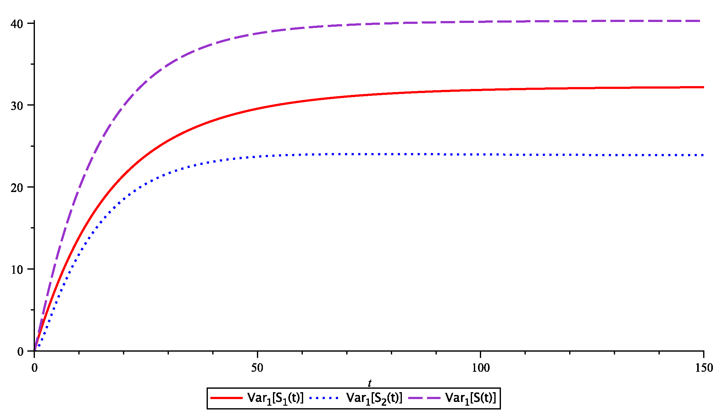
Figure 1 plots the variances of $S\left(t\right),S_1\left(t\right),$ and $S_2\left(t\right)$, given $J\left(0\right)=1,$ for $0\le t\le 150.$ The variances all increase with time t. The variance of $S\left(t\right)$ is bigger than those of $S_1\left(t\right)$ and $S_2\left(t\right)$ for a fixed t. When time t goes to $\infty ,$ the three variances converge.

Table 2. Covariances of discounted claims at t and $t+1$.

t	$\mathit{J}\left(0\right)=1$
	${\mathbf{Cov}}_1\left(\mathit{S}\left(\mathit{t}\right),\mathit{S}(\mathit{t}+1)\right)$	${\mathbf{Cov}}_1({\mathit{S}}_1\left(\mathit{t}\right),{\mathit{S}}_1(\mathit{t}+1))$	${\mathbf{Cov}}_1({\mathit{S}}_2\left(\mathit{t}\right),{\mathit{S}}_2(\mathit{t}+1))$
1	$1.9327$	$1.7143$	$0.5328$
2	$3.9024$	$3.2169$	$1.7021$
5	$9.5545$	$7.3372$	$5.8448$
10	$17.0771$	$12.8965$	$11.4471$
20	$26.6637$	$20.2686$	$18.0782$
30	$31.9796$	$24.5961$	$21.2571$
∞	$40.3073$	$32.2449$	$23.8648$

and

Table 3. Covariances of discounted claims at t and $t+5$.

t	$\mathit{J}\left(0\right)=1$
	${\mathbf{Cov}}_1\left(\mathit{S}\left(\mathit{t}\right),\mathit{S}(\mathit{t}+5)\right)$	${\mathbf{Cov}}_1({\mathit{S}}_1\left(\mathit{t}\right),{\mathit{S}}_1(\mathit{t}+5))$	${\mathbf{Cov}}_1({\mathit{S}}_2\left(\mathit{t}\right),{\mathit{S}}_2(\mathit{t}+5))$
1	$0.8651$	$1.2213$	$0.4437$
2	$1.3181$	$2.0228$	$1.4775$
5	$3.4481$	$4.5219$	$5.2676$
10	$7.5945$	$8.5121$	$10.5187$
20	$15.2651$	$14.9882$	$16.9435$
30	$21.6039$	$19.7868$	$20.2186$
∞	$40.3073$	$32.2449$	$23.8648$

display the covariances of the ADC at time t and $t+h$, given $J\left(0\right)=1$, for some selected t values and for $h=1$ and $h=5$. It is shown that $S\left(t\right)$ and $S(t+h),$$S_1\left(t\right)$ and $S_1(t+h),$ and $S_2\left(t\right)$ and $S_2(t+h)$ are all positively correlated. Moreover, when t increases, the covariances increase; moreover, when h increases, the covariances decrease. When $t\to \infty ,$ the covariances of the pairs $S\left(t\right)$ and $S(t+h)$, $S_i\left(t\right)$, and $S_i(t+h)$ converge to the variances of $S(\infty )$ and $S_i(\infty )$, respectively. Similar patterns should be expected for $J\left(0\right)=2.$

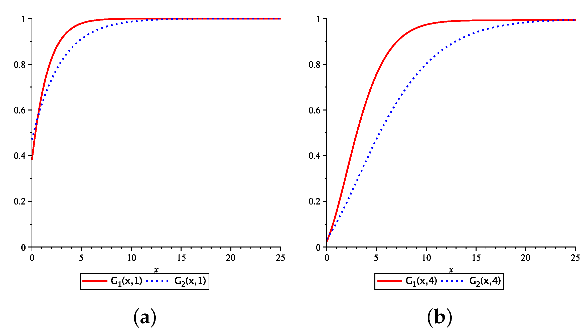
Finally, we display in Figure 2 the numerical values of the distribution function of $S\left(t\right)$ with initial state i, $G_i(x,t)={\mathbb{P}}_i(S\left(t\right)\le x)$, for $t=1$ and 4, $0\le x\le 25$, and $i=1,2$. Note that $\mathbf{G}(x,t)={(G_1(x,t),G_2(x,t))}^{\top }$ satisfies the partial differential Equation (25); its solution can be obtained numerically. From the graph, it shows clearly that the probability of $S\left(t\right)$ being bigger than a fixed x is smaller for small values of t as expected. For most x values, $G_1(x,t)$ is bigger than $G_2(x,t)$ due to the fact that the underlying Markov process in our example tends to stay in state 1 more often than staying at state 2.

References

- Asmussen, Søren. 2003. Applied Probability and Queues. New York: Springer. [Google Scholar]
- Barges, Mathieu, Hélene Cossette, Stéphane Loisel, and Etienne Marceau. 2011. On the moments of the aggregate discounted claims with dependence introduced by a FGM copula. ASTIN Bulletin 41: 215–38. [Google Scholar]
- Delbaen, Freddy, and Jean Haezendonck. 1987. Classical risk theory in an economic environment. Insurance: Mathematics and Economics 6: 85–116. [Google Scholar] [CrossRef]
- Garrido, José, and Ghislain Léveillé. 2004. Inflation impact on aggregate claims. Encyclopedia of Actuarial Science 2: 875–78. [Google Scholar]
- Kim, Bara, and Hwa-Sung Kim. 2007. Moments of claims in a Markov environment. Insurance: Mathematics and Economics 40: 485–97. [Google Scholar]
- Jang, Ji-Wook. 2004. Martingale approach for moments of discounted aggregate claims. Journal of Risk and Insurance 71: 201–11. [Google Scholar] [CrossRef]
- Leveille, Ghislain, and Franck Adekambi. 2011. Covariance of discounted compound renewal sums with stochastic interest. Scandinavian Actuarial Journal 2: 138–53. [Google Scholar] [CrossRef]
- Léveillé, Ghislain, and Franck Adékambi. 2012. Joint moments of discounted compound renewal sums. Scandinavian Actuarial Journal 1: 40–55. [Google Scholar] [CrossRef]
- Leveille, Ghislain, and Jose Garrido. 2001a. Moments of compound renewal sums with discounted claims. Insurance: Mathematics and Economics 28: 201–11. [Google Scholar]
- Léveillé, Ghislain, and José Garrido. 2001b. Recursive moments of compound renewal sums with discounted claims. Scandinavian Actuarial Journal 2: 98–110. [Google Scholar] [CrossRef]
- Léveillé, Ghislain, José Garrido, and Ya Fang Wang. 2010. Moment generating functions of compound renewal sums with discounted claims. Scandinavian Actuarial Journal 3: 165–84. [Google Scholar] [CrossRef]
- Li, Shuanming. 2008. Discussion of "On the Laplace transform of the aggregate discounted claims with Markovian arrivals". North American Actuarial Journal 12: 208–10. [Google Scholar] [CrossRef]
- Li, Jingchao, David CM Dickson, and Shuanming Li. 2015. Some ruin problems for the MAP risk model. Insurance: Mathematics and Economics 65: 1–8. [Google Scholar] [CrossRef]
- Mohd Ramli, Siti Norafidah, and Jiwook Jang. 2014. Neumann series on the recursive moments of copula-dependent aggregate discounted claims. Risks 2: 195–210. [Google Scholar] [CrossRef] [Green Version]
- Neuts, Marcel F. 1979. A versatile Markovian point process. Journal of Applied Probability 16: 764–79. [Google Scholar] [CrossRef]
- Ren, Jiandong. 2008. On the Laplace transform of the aggregate discounted claims with Markovian arrivals. North American Actuarial Journal 12: 198–206. [Google Scholar] [CrossRef]
- Taylor, Gregory Clive. 1979. Probability of ruin under inflationary conditions or under experience rating. ASTIN Bulletin 10: 149–62. [Google Scholar] [CrossRef]
- Wang, Ya Fang, José Garrido, and Ghislain Léveillé. 2018. The distribution of discounted compound PH-renewal processes. Methodology and Computing in Applied Probability 20: 69–96. [Google Scholar] [CrossRef]
- Willmot, Gordon E. 1989. The total claims distribution under inflationary conditions. Scandinavian Actuarial Journal 1: 1–12. [Google Scholar] [CrossRef]
- Woo, Jae-Kyung, and Eric CK Cheung. 2013. A note on discounted compound renewal sums under dependency. Insurance: Mathematics and Economics 52: 170–79. [Google Scholar] [CrossRef]
Figure 1.
Variances of , and with initial state .
Figure 2.
Distribution functions of in (a) and in (b) for