The Effect of Non-Proportional Reinsurance: A Revision of Solvency II Standard Formula


Department of Mathematics, Finance and Econometrics, Università Cattolica del Sacro Cuore, Largo Gemelli 1, 20123 Milano, Italy
Risks 2018, 6(2), 50; https://doi.org/10.3390/risks6020050
Submission received: 26 March 2018
/
Revised: 22 April 2018
/
Accepted: 25 April 2018
/
Published: 2 May 2018
(This article belongs to the Special Issue Capital Requirement Evaluation under Solvency II framework)
Abstract
:Solvency II Standard Formula provides a methodology to recognise the risk-mitigating impact of excess of loss reinsurance treaties in premium risk modelling. We analyse the proposals of both Quantitative Impact Study 5 and Commission Delegated Regulation highlighting some inconsistencies. This paper tries to bridge main pitfalls of both versions. To this aim, we propose a revision of non-proportional adjustment factor in order to measure the effect of excess of loss treaties on premium risk volatility. In this way, capital requirement can be easily assessed. As numerical results show, this proposal appears to be a feasible and much more consistent approach to describe the effect of non-proportional reinsurance on premium risk.
1. Introduction
Solvency II is changing the way regulatory capital is assessed in European countries. Despite clear challenges, the new framework also offers insurers the possibility to improve business strategy and capital allocation. In this context, risk mitigation appears as a key driver.
For most companies, regulatory capital requirements have historically played a relatively small role in the decision to purchase a particular reinsurance contract. However, the main results of quantitative impact studies have showed that capital requirements under Solvency II are likely to increase substantially for most non-life insurers.
Although, at the moment, it is far from becoming the dominant factor in a reinsurance purchasing decision (see Wills Re (2017) for a survey on this point), the impact of the reinsurance in Solvency II capital assessment should be explored. The capital requirement being more risk-based than in the past, it will likely become, among others, an important factor in the selection of reinsurance contracts. In this regard, a growing influence of risk appetite is observed, helping insurance companies navigate reinsurance coverage options (Wills Re (2017)).
Under the standard formula (see European Commission (2015)), the capital relief for non-life underwriting risk is easily determined by multiplying by the ceded percentage for proportional reinsurance (as quota share). For non-proportional reinsurance, the capital saving effect is less immediately apparent, and it is mainly based on the evaluation of a non-proportional factor given by European Insurance and Occupational Pensions Authority (EIOPA). In particular, the standard formula defines the methodology for assessing the non-proportional factor, subject to specific limitations and criteria. This factor should quantify the mitigation of total losses’ variability given by excess of loss (XL) treaties.
This paper raises a number of key considerations and complexities in the recognition of reinsurance mitigation in the standard formula and partial internal models, including concerns surrounding the quantification of the capital reduction1.
We show how the solution provided by Solvency II is not consistent with collective risk theory (see Beard et al. (1984), Daykin et al. (1994), and Klugman et al. (2008)) commonly used for premium risk evaluation. In this regard, as shown in Daykin et al. (1994), Gisler (2009), and Savelli and Clemente (2009), a systematic component usually affects the number of claims. We prove that both formulae provided by the Commission Delegated Regulation (or delegated acts—DA) (European Commission (2015)) and quantitative impact study 5 (QIS5) (European Commission (2010)) neglect this component, leading to an overestimation of the risk mitigating effect. This result is clearly relevant from the supervisor’s perspective. Additionally, the size of the insurers is not taken into account. As is well known, because of a different pooling risk between small and large insurers, the impact of XL reinsurance could be substantially different. Furthermore, the approach provided by the standard formula being based on a lognormal assumption (Clark (1996), Coutts and Thomas (1997a), Coutts and Thomas (1997b)), the shape of the distribution of net aggregate claims is proportional to the relative volatility. Focusing the XL treaty on the right tail of the claim-size distribution, it should be evaluated if the mitigation of skewness is greater than the reduction of volatility.
In order to overcome these pitfalls, we provide a fruitful solution to measure the effect of XL treaties on the variability coefficient of the aggregate claim amount. We show how the methodology is consistent with the Solvency II standard formula and how it could be a viable alternative to existing specific approaches. For the sake of brevity, we focus here only on XL treaties, but the approach can also be easily extended to other non-proportional strategies (as stop-loss).
In particular, in Section 2, some preliminaries are given. Section 3 and Section 4 describe methods provided in QIS5 and DA respectively to evaluate non-proportional reinsurance. An alternative solution to this problem is given in Section 5. Finally some numerical results are reported in Section 6 in order to compare alternative approaches considering a multi-line non-life insurer. Furthermore, we show how main characteristics, such as the portfolio size, pooling risk, and portfolio mix can affect the results. Conclusions follow.
2. Some Notations and Preliminaries
We introduce here some general results that are used in the next sections. We define the random variable (r.v.) 2 as the aggregate amount of next year’s (paid and reserved) claims of a single line of business (LoB). Adopting the well-known collective risk-theoretic model (see Beard et al. (1984), Bühlmann (1970), and Daykin et al. (1994)), this r.v. may be expressed as
where we have the following:
- is a r.v. denoting the claim count. As is usually provided in literature (see Daykin et al. (1994) and Savelli and Clemente (2009)), the number of claims’ distribution follows the Poisson law (), with an expected number of claims n disturbed by a structure variable .
- is a mixing variable (or contagion parameter) (see Gisler (2009), Meyers and Shenker (1982), and Savelli and Clemente (2009)) that describes the parameter uncertainty on the number of claims. It is assumed that and that the r.v. is defined only for positive values.
- is the amount of the claim h (severity). As usual, are mutually independent and identically distributed r.v.’s, each independent of the number of claims . We denote with raw moments of order j.
In order to focus only on premium risk, we consider next year’s incurred losses that can be covered by using earned premiums. We exclude payments for claims that had already occurred at the valuation date, because this r.v. is treated in reserve risk evaluation. Furthermore, previous assumptions are based on a mixed compound Poisson process that is a classical methodology used in literature and in practice to quantify the capital requirement for premium risk.
By knowing the well-known relation of the cumulative generating function (c.g.f.) of total losses (see Daykin et al. (1994)):
the main cumulants of can be computed (see Savelli and Clemente (2009)).
Here we recall that the coefficient of variation (CV) of the aggregate claim amount () is equal to
where is the variance of r.v. , and is the coefficient of variation of the severity distribution.
We note that is composed by a fluctuation risk that decreases with the size of the company and a parameter risk that is independent of the size.
3. Non-Proportional Reinsurance in QIS5
The purpose of this section is to describe the main features of the QIS5 standard formula as they would apply to a property/casualty insurer. As this paper deals with non-proportional reinsurance, we focus on the premium and reserve risk sub-module. The capital charge is obtained as
where measures the distance between the 99.5% quantile and the mean of the distribution of the r.v. derived as the ratio of total losses divided by the volume measure V related to both premium and reserve risk for all the LoBs.
The function is set equal to , and it has been calibrated under the assumption of a lognormal distribution. V takes into account both the expected earned next-year premiums and the value of the best estimate of the claims reserve at the valuation date. Both amounts are considered the net of reinsurance.
represents instead the standard deviation of the r.v. previously defined in relation to the overall non-life portfolio. The overall is derived by obtaining the standard deviation of each risk and LoB i ( and ) and aggregating them through a two-step procedure. We have indeed an initial aggregation between the premium and reserve risk of a single LoB assuming a correlation coefficient of 0.5, and then the standard deviations of different LoBs are aggregated by using a fixed correlation matrix.
To this aim, following relation holds:
where is the correlation matrix between different LoBs given by QIS5 (European Commission (2010)), and with n being the number of LoBs. For each LoB i, we have
The standard deviations and may be derived by using alternatively a given market-wide estimate or an undertaking-specific approach based on fixed methodologies3 applied to insurer’s data.
Only for premium risk can the market-wide estimates be reduced using a formula to reflect the extent the ceded reinsurance is non-proportional reinsurance. is indeed equal to a fixed volatility factor (e.g., 10% for motor third-party liabilities (MTPL)) multiplied by a non-proportional factor that allows for risk-mitigating effects of per risk XL reinsurance. Undertakings may choose for each LoB to set the adjustment factor to 1 or to calculate it as set out in the QIS5 technical specifications (TS) (European Commission (2010)).
If the XL treaty meets the requirement requested by TS4, may be derived as
where and are the mean and the standard deviation of the gross claim severity distribution evaluated by using loss experience. and are instead the net (of reinsurance) values. The effect of the reinsurance retention (and limit) is evaluated by assuming a lognormal distribution of individual losses.
We note that Equation (6) measures the net-to-gross ratio of variability coefficients of total losses. The same relation can be found by applying Equation (2) under the assumption that the total losses are described by a pure compound Poisson process (i.e., and consequently ). We have that disregards the effect of parameter uncertainty on the claim count and is instead a systematic component that cannot be reduced by XL reinsurance. We show in Section 6 how this assumption can overestimate the effect of reinsurance treaties, leading to a significant capital relief.
Furthermore, if we restrict the analysis to premium risk of a single LoB, Equation (3) can be rewritten as
where and are the net and gross coefficients of variation of the total losses under a pure compound Poisson process (as assumed in QIS5).
Other than neglecting parameter risk, it is noteworthy that Equation (7) shows further implicit assumptions regarding reinsurance:
- The standard deviation of the ratio of gross losses to gross premiums is modified to take into account XL through the net-to-gross ratio of coefficients of variation: . QIS5 implicitly assumes that expected losses decrease in the same proportion as the volume measure after reinsurance: . In other words, Equation (7) assumes that loading coefficients of the reinsurer are equal to loading coefficients of the cedent.
- The size of insurers’ portfolio is not considered. Risk mitigation usually has a different effect because of a different weight of pooling and non-pooling risk (see, e.g., International Actuarial Association (2004)).
- Both the gross and net reinsurance distributions are assumed as lognormal. The skewness of this distribution being strictly related to the coefficient of variation5, QIS5 assumes that skewness reduces in a similar way to CV () for usual volatilities. The XL acting on the tail of the severity distribution, it should be evaluated if the mitigation of skewness is greater than the mitigation of volatility.
4. Non-Proportional Reinsurance in Commission Delegated Regulation
The evaluation of the premium and reserve sub-module was slightly modified by the Technical Specifications of the Long-Term Guarantee Assessment in 2013. Changes have been confirmed by the Commission Delegated Regulation (or DA) (European Commission (2015)) approved by the European Commission. This is the final version of the standard formula of Solvency II applied by the insurers for the solvency assessment in 2016 and 2017 balance sheets6. The general approach is always based on a factor-based formula in which the standard deviation of each LoB and risk is derived by means of either a market-wide or an undertaking-specific approach. Standard deviations are then aggregated by applying Equations (4) and (5) on the basis of the same correlation matrices used in QIS5. The overall standard deviation is used to quantify the capital charge via the following relation:
where the function has been replaced by a fixed multiplier equal to 3.
This assumption tends to simplify the calculations, but it does not take into account the skewness of the distribution of losses, assuming always the same ratio of the 99.5% quantile less the mean divided by the standard deviation. It gives the same result as the function used in QIS5 only when is around 14.5%. This choice tends to underestimate capital requirement for small insurers and overestimate it for larger insurers, with respect to the assumption of a lognormal distribution of total losses.
Furthermore, the market-wide estimates of the standard deviation of the premium risk are based on a gross volatility multiplied by a adjustment factor. DA provides a different estimation of . In particular, the undertaking-specific adjustment factor for non-proportional reinsurance is derived through the following credibility formula:
where is a fixed value equal to 80% in MTPL, motor own damages (MOD), and property LoBs only if XL treaties are in force. It is equal to 1 for all other segments; c is a credibility coefficient depending by the length of available time series. A minimum of 5 years is required to have a value of c greater than zero. This is instead equal to 1 when data over at least 10 years are available. For MTPL, property, and general third-party liabilites (GTPL), at least 15 years are requested to have full credibility.
Finally can be estimated by insurers’ data as the square root of the net-to-gross ratio of second raw moments of severity distributions:
The gross amount is estimated by data, while the net amount is derived by evaluating the effect of reinsurance retention on a lognormal distribution. The same approach is adopted in cases for which the recognizable excess of the loss reinsurance contract provides compensation only up to a specified limit.
Equation (10) appears to be a stronger approximation than QIS5. The gross volatility factor , which measures a relative variability, is reduced by means of the risk mitigation effect on the second raw moment of the claim size. Under a compound pure Poisson process, measures the net-to-gross ratio of the standard deviations of the total losses. Indeed, considering only one LoB and only premium risk, DA assumes in the case of full credibility () that
where and are the net and gross standard deviations of the total losses under a pure compound Poisson process.
Furthermore, it is noteworthy that DA implicitly assumes that reinsurance does not affect the skewness of distribution. Equation (8) obtains the distance between the 99.5% quantile and the mean as 3 times the standard deviation in both net and gross cases.
5. A Proposal of an Alternative Non-Proportional Factor
As detailed in the previous sections, both QIS5 and DA approaches derive the net volatility of each LoB by multiplying the gross risk factor by a non-proportional factor. A crucial point is the calibration of this factor. In order to overcome some pitfalls of both QIS5 and DA proposals, we provide here a different formula. The volatility factor being defined as the ratio of the total losses to the volume measure, we can compute the net volatility as
where .
We assume that a mixed compound Poisson process describes the aggregate number of claims. It is noteworthy that Equation (12) allows for the effect of a systematic component on the claim count, neglected by QIS5 and DA, that is not affected by the XL reinsurance treaty. Furthermore, also depends on both the net-to-gross risk premium ratio and the net-to-gross volume ratio. The last two terms are equal to 1 only if the reinsurer underwrites with a percentage of premium loadings equal to the insurer. The proposed formula overcomes the main pitfalls of the coefficients provided in QIS5 and DA, and it allows us to derive net volatilities of premium risk for each LoB. By replacing these new volatilities in Equation (5) and by applying Equations (3) and (4), capital requirement can be easily obtained. In this way, we agree with the lognormal assumption given in QIS5.
The validity of the result may be called into question if the application of the lognormal distribution fails to conform adequately to experience. In order to numerically check this proposal, we also derive the skewness of the net total losses’ distribution under a mixed compound Poisson process. By using c.g.f. of total losses, we have:
where are risk factors of order j, evaluated for the net of reinsurance. This result allows us to validate the lognormal assumption for a single LoB. The problem of evaluating the skewness of the aggregate portfolio may be satisfactorily addressed only by assuming the structure of dependence between different LoBs. In the numerical section, we test the lognormal assumption by modeling the dependence via Gaussian copulas.
6. Some Examples of Numerical Impact
In order to compare our proposal to the capital requirements derived by QIS5 and DA, we consider a standard non-life insurer. The main figures are summed up in Table 1, where gross characteristics are reported. The insurer’s portfolio is structured around three LoBs: MTPL, GTPL, and MOD, with a prominent weight of MTPL. As detailed in the following, next-year premiums have been estimated assuming an annual increase of 5% with respect to earned premiums of the previous year. This increase was the standard assumption on annual premiums’ growth in quantitative impact studies. No multi-year policies are present. Best estimates of claims reserves posted by the insurer at the end of year are also reported in Table 1. We observe the significant number of claims reserves because two long-tail LoBs are considered. Furthermore, we assume that the insurer wishes to reinsure a part of his portfolio in order to reduce its volatility. To investigate the effect of non-proportional factors on the premium risk capital requirement, we consider XL treaties, varying the reinsurance limits for each LoB.
Table 2 reports the observed number of claims (n) and average cost per claim (m). These values, together with the assumptions on the real growth rate of the portfolio (g) and on the claim inflation rate (i), allow us to estimate the risk premiums for next year, . It has to be pointed out that some key parameters, such as the safety loading coefficient () on the risk premium and the standard deviation of the structure variable (), are obtained mainly by Italian market loss ratios and combined ratios for the period 1999–2013. A negative safety loading coefficient is used when the observed combined ratio is greater than 1 (e.g., in GTPL). Furthermore, expenses’ loadings (c) have been calibrated by using the historical pattern of both management and acquisition expenses in the same period. Next-year premiums have been derived as . For the sake of simplicity, we take into account only new business and annual contracts. Finally, in order to reflect variability of LoBs, we consider the coefficient of variation of the claim size (), estimated by using the empirical distribution of individual losses.
These calibrations7 allow a realistic analysis of the effect of non-proportional reinsurance on the capital requirement in order to assure a consistent comparison between alternative approaches.
We focus initially on the premium risk volatility of each LoB. Subsequently, we assess the total capital requirement in order to evaluate the risk mitigation effect also on an aggregated basis.
To assure a consistent comparison, we assume that the retention limit of the XL treaty is equal to the sum of the average claim cost and a fixed multiplier S of the standard deviation: . S is initially set equal to 15. In this scenario, the attachment point is roughly 400,000 euro for MTPL, 1.5 million euro for GTPL, and 80,000 euro for MOD. We report in Table 3 the non-proportional factor derived by applying QIS5, DA and Equation (12). Equation (12) has been evaluated by assuming that the reinsurer has a safety loading coefficient either equal to (see ) or greater than the ceding company (see ). In the second case, the reinsurer’s safety loading has been derived by taking into account the reduction in the variability of the cedent. Finally, we give full credibility () to the undertaking-specific methodology when DA is applied (i.e., ).
We may observe (see Table 3) that QIS5 and DA lead to similar adjustment factors. It is noteworthy that the standard formula tends to overestimate the risk mitigation effect because non-pooling risk is ignored. gives instead greater values because of parameter risk (i.e., effect). In particular, long-tail LoBs (such as GTPL and MTPL) show a significant underestimation of under the Solvency II criteria. Additionally, the fixed value of 80% allowed by DA for MTPL and MOD also appears not to be a prudential choice. Finally, the non-proportional factor has been evaluated in order to also consider reinsurer pricing (). A slight reduction in the factor is observed when the reinsurer applies a safety loading greater than that of the insurer.
In a similar fashion, Figure 1 reports the values of the volatility factor of the premium risk for the LoBs analyzed. As expected, we observe how the methodology proposed by both QIS5 and DA leads to a significant reduction in the volatility factor.
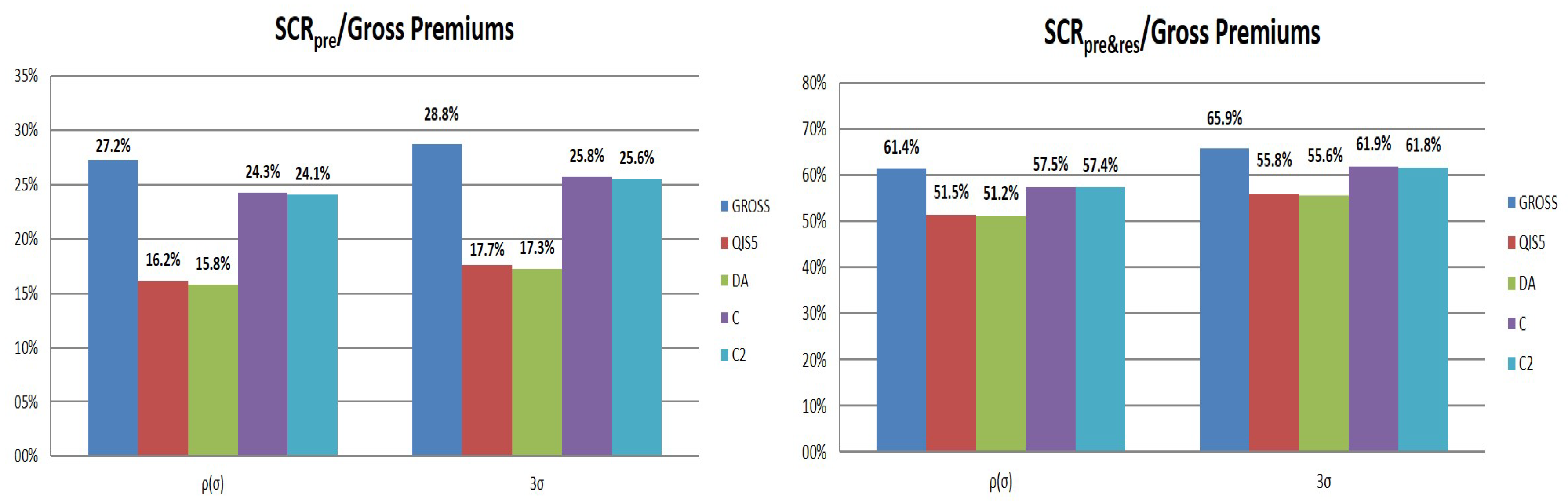
Figure 2 reports instead the Solvency Capital Requirement (SCR) ratios (SCR divided by initial gross premiums) considering either only premium risk or both premium and reserve risk. Capital requirements have been derived using only a market-wide approach, by testing alternative formulae for the non-proportional factor and by considering both and versions proposed by QIS5 and DA, respectively (see Equations (3) and (8)).When reinsurance is not considered, the premium risk capital charge is equal to 27% of premiums under the lognormal assumption and to 29% with the DA approach. Also taking into account reserve risk, we observe ratios of 61% and 66%. It is emphasized how lower volatilities lead to higher differences between the two approaches. The gross is indeed equal to 7.6% when both the premium and reserve are considered, while it is equal to 9% when only premium risk is present.
Considering the risk mitigation effect of XL treaties, both QIS5 and DA allow us to save roughly 40% of the capital requirement for premium risk. As is well known, the market-wide approach does not consider the effect of reinsurance on the reserve risk volatility, leading to a saving of capital cost of about 16% for the premium and reserve sub-module.
A limited effect is indeed recognized under and criteria because the systematic component of the claim count is not affected by the treaty. In this case, net-to-gross capital ratios are equal to roughly 90% and 94% when either only premium risk or also reserve risk is taken into account.
In order to better analyze the effect on the non-proportional factor of the insurer’s characteristics, we develop a sensitivity analysis suitable to identify critical parameters. In this regard, Figure 3 shows values of evaluated considering alternative coefficients of variation of the severity distribution. As expected, higher variabilities lead to an increasing effect of non-proportional reinsurance. Although this result is apparent, we observe how the overestimation of the risk mitigation effect recognized by the standard formula increases for higher values of . Only when very low relative volatilities are considered do all the methodologies provide similar values of close to 1.
The parameter uncertainty () on the claims count has been tested and is shown in Figure 4. While QIS and DA are not affected by this systematic component, the effect of XL should decrease, the pooling risk being neglectable (as shown by and results).
Furthermore, the portfolio size is not even considered in the standard formula, leading to the same risk mitigation for small and large companies (see Figure 5). Generally, small companies show a higher relative saving of capital when XL treaties are in force (see, e.g., Appendix B on non-life insurance of International Actuarial Association (2004)). As both and show, this effect increases for LoB with a higher or a lower because of the more relevant pooling risk.
We also evaluate the effect of a different retention limit (see Figure 6). The attachment point has been evaluated as , where alternative values of S have been tested (see also De Lourdes Centeno (1995) for an analysis of the effect of retention limit on risk reserve). As expected, a greater retention limit leads to a reduction in . Also in this analysis, the overestimation of the risk mitigation effect when the standard formula is applied has been confirmed. In particular, it is noteworthy that the standard formula also provides, for higher retentions, a non-proportional factor significantly lower than 1. For example, when S is equal to 100, attachment points are equal to roughly 2.5 million euro for MTPL, 10.3 million euro for GTPL, and 0.5 million euro for MOD. Although very high limits, the evaluated by the standard formula is equal to roughly 88% for MTPL, 77% for GTPL, and 99.5% for MOD with a significant capital relief.
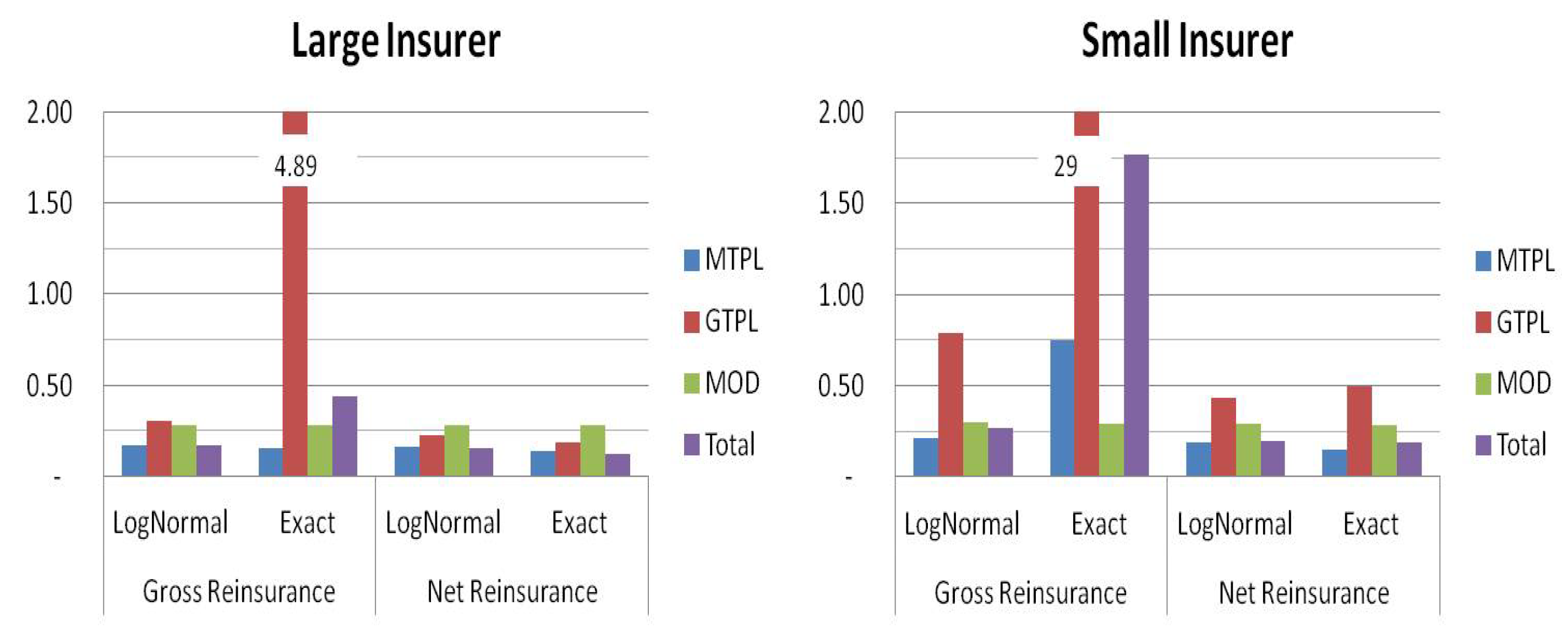
Finally, in order to test the lognormal assumption of the net total losses, we analyze the skewness of this r.v. To this end, we compare the skewness of the lognormal distribution to the exact distribution provided by Equation (13). Furthermore, to evaluate the skewness of the total portfolio, the dependence is described by a Gaussian copula calibrated through the standard formula correlation matrix. The comparison regards both the insurer, whose characteristics are reported in Table 1, and a smaller insurer, whose portfolio is 1/10 of the larger portfolio. Figure 7 shows how the lognormal assumption tends to underestimate real skewness for small portfolios or highly volatile businesses (such as GTPL). However, for both companies, this assumption seems consistent when we analyze the net of the reinsurance distribution.
7. Conclusions
As is well known, reinsurance is a powerful risk mitigating tool for insurance undertakings, particularly non-proportional reinsurance, which allows insurance companies to transfer significant parts of tail risks to reinsurers at a given price.
The Solvency II standard formula provides a specific methodology to evaluate the risk mitigating effect of non-proportional reinsurance on the capital requirement for premium risk. We show some inconsistencies of both versions proposed in QIS5 and DA. In particular, we emphasize how the underlying assumptions can overestimate the impact of XL treaties, leading to a significant saving of capital. Furthermore, from a methodological point of view, the final formula approved is also worse than the QIS5 proposal. We provide an extension of this methodology that could be used for a revision of the Solvency II standard formula. By a detailed sensitivity analysis, we show how the proposal tends to be more consistent with classical approaches of risk theory, allowing it to overcome main drawbacks of the undertaking-specific approach provided by the standard formula.
References
Conflicts of Interest
The author declares no conflict of interest.
References
- Beard, R. E., T. Pentikäinen, and E. Pesonen. 1984. Risk Theory, 3rd ed. London: Chapman & Hall. [Google Scholar]
- Bühlmann, Hans. 1970. Mathematical Methods in Risk Theory. New York: Springer. [Google Scholar]
- Clark, David R. 1996. Basics of Reinsurance Pricing. CAS Study Notes 41–43: 1–52. [Google Scholar]
- Clemente, Gian Paolo, Nino Savelli, and Diego Zappa. 2015. The Impact of Reinsurance Strategies on Capital Requirements for Premium Risk in Insurance. Risks 3: 164–82. [Google Scholar] [CrossRef]
- Clemente, Gian Paolo, and Nino Savelli. 2017. Actuarial Improvements of Standard Formula for Non-Life Underwriting Risk. In Insurance Regulation in the European Union Solvency II and Beyond. Basingstoke: Palgrave Macmillan. [Google Scholar]
- Coutts, Stewart M., and Timothy R. H. Thomas. 1997a. Capital and risk and their relationship to reinsurance programmes. Paper presented at 5th International Conference on Insurance Solvency and Finance, London, UK, June 17. [Google Scholar]
- Coutts, Stewart M., and Timothy R. H. Thomas. 1997b. Modelling the impact of reinsurance on financial strength. British Actuarial Journal 3: 583–653. [Google Scholar] [CrossRef]
- Daykin, Chris D., Teivo Pentikäinen, and Martti Pesonen. 1994. Practical Risk Theory for Actuaries, Monographs on Statistics and Applied Probability 53. London: Chapman & Hall. [Google Scholar]
- De Lourdes Centeno, Maria. 1995. The effect of the retention limit on risk reserve. ASTIN Bulletin 25: 67–74. [Google Scholar] [CrossRef]
- EIOPA. 2017. Consultation Paper on EIOPA’s First Set of Advice to the European Commission on Specific Items in the Solvency II Delegated Regulation. Technical Report. Frankfurt: European Insurance and Occupational Pensions Authority (EIOPA). [Google Scholar]
- EIOPA. 2018. Consultation Paper on EIOPA’s Second Set of Advice to the European Commission on Specific Items in the Solvency II Delegated Regulation. Technical Report. Frankfurt: European Insurance and Occupational Pensions Authority (EIOPA). [Google Scholar]
- European Commission. 2015. Commission Delegated Regulation (EU) 2015/35 supplementing Directive 2009/138/EC of the European Parliament and of the Council on the taking-up and pursuit of the business of Insurance and Reinsurance (Solvency II), 10 of October 2014. Official Journal of the EU 58: 1–797. [Google Scholar]
- European Commission. 2010. Quantitative Impact Study 5—Technical Specifications. Brussels: European Commission. [Google Scholar]
- Gisler, Alois. 2009. The Insurance Risk in the SST and in Solvency II: Modelling and Parameter Estimation. Helsinki: Astin Colloquium. [Google Scholar]
- Hurlimann, Werner. 2005. Excess of loss reinsurance with reinstatements revisited. Astin Bulletin 35: 211–38. [Google Scholar] [CrossRef]
- Klugman, Stuart A., Harry H. Panjer, and Gordon E. Wilmot. 2008. Loss Models: From Data to Decisions, 3rd ed. Wiley Series in Probability and Statistics; Hoboken: John Wiley & Sons. [Google Scholar]
- International Actuarial Association. 2004. A Global Framework for Insurer Solvency Assessment. Report of Insurer Solvency Assessment Working Party. Ottawa: International Actuarial Association. [Google Scholar]
- Meyers, Glenn, and Nathaniel Shenker. 1982. Parameter Uncertainty in the Collective Risk Model, Casualty Actuarial Society, Discussion Paper Program. pp. 253–300. Available online: https://www.casact.org/pubs/proceed/proceed83/83111.pdf (accessed on 1 May 2018).
- Savelli, Nino, and Gian Paolo Clemente. 2011. Hierarchical Structures in the aggregation of Premium Risk for Insurance Underwriting. Scandinavian Actuarial Journal 3: 193–213. [Google Scholar] [CrossRef]
- Savelli, Nino, and Gian Paolo Clemente. 2009. Modelling Aggregate Non-Life Underwriting Risk: Standard Formula vs Internal Model. Giornale dell’Istituto Italiano degli Attuari 72: 301–38. [Google Scholar]
- Wills Re. 2017. Global Reinsurance and Risk Appetite Report. Technical Report. Available online: http://www.willisre.com/documents/Media_Room/Publication/Willis%20Re%20Global%20Reinsurance%20and%20Risk%20Appetite%20Survey%202017.pdf (accessed on 1 May 2018).
| 1. | For comments about main drawbacks in the quantification of the capital requirement in non-life insurance, see also Clemente and Savelli (2017). |
| 2. | In the following, a tilde indicates random variables. |
| 3. | Three alternative methodologies are provided in QIS5 for both premium and reserve risk. |
| 4. | |
| 5. | Given a random variable distributed as lognormal, we have that skewness is . |
| 6. | |
| 7. | Similar approaches for the calibration of parameters have been used in Clemente et al. (2015) and Savelli and Clemente (2011). |
Figure 1.
Gross and net values of premium risk volatilities ().
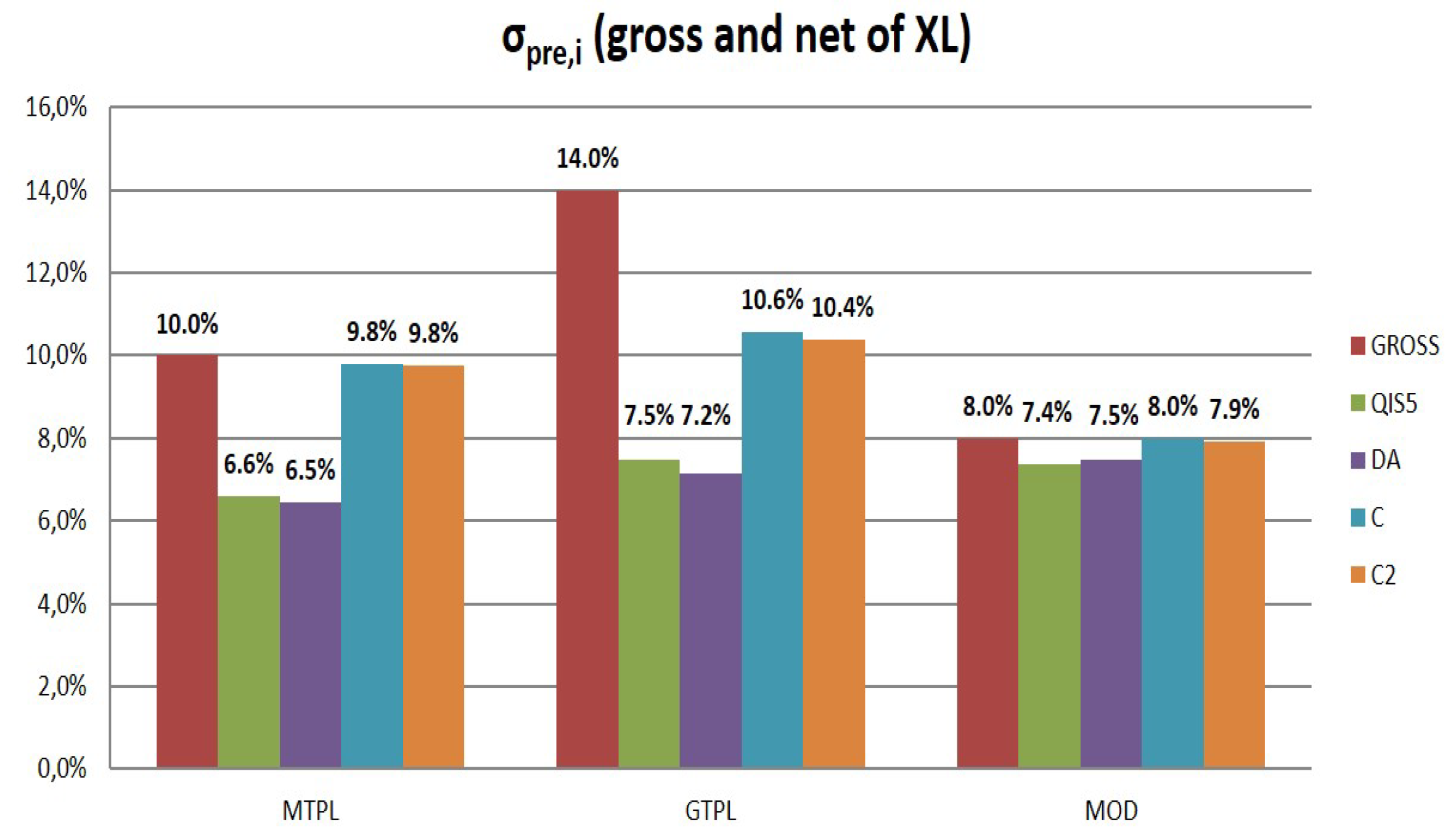
Figure 2.
Ratios between SCR and initial gross premiums.

Figure 3.
according to several coefficients of variation of claim size ().
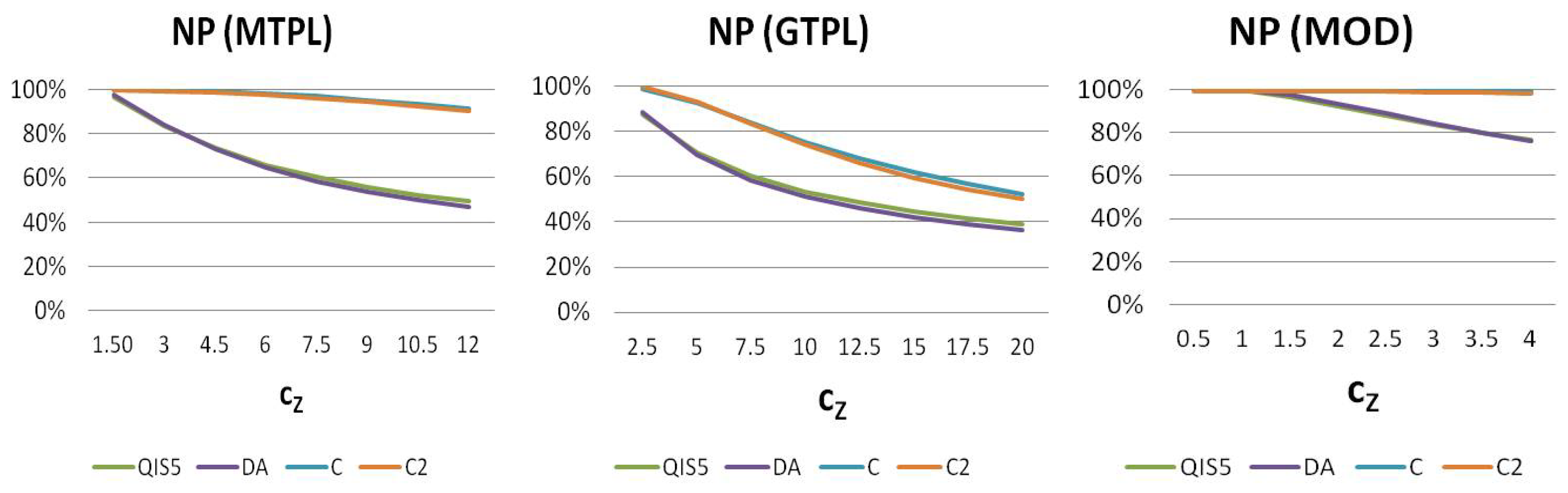
Figure 4.
according to several values of standard deviation of structure variable ().
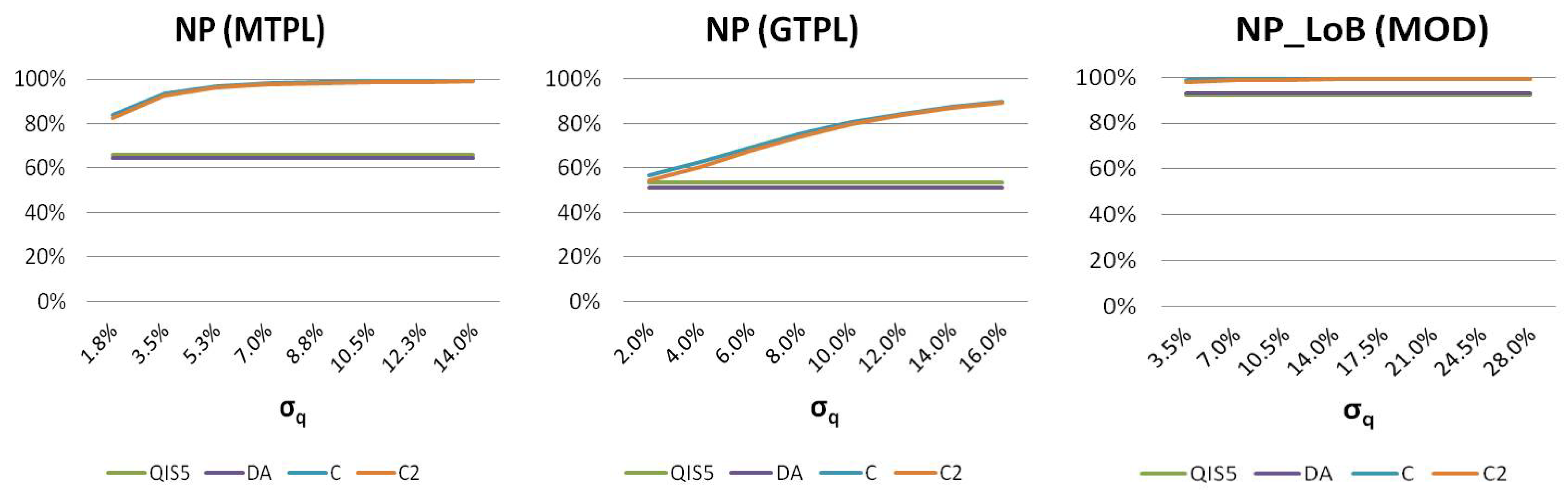
Figure 5.
according to several values of expected claims count (n).
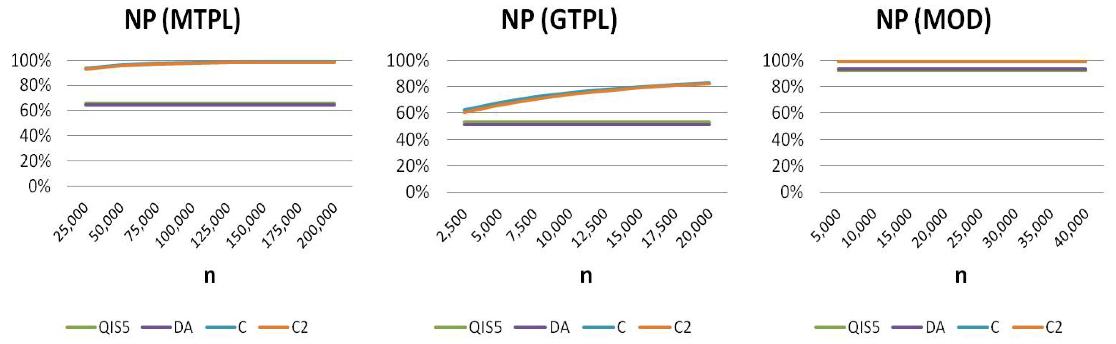
Figure 6.
according to different retention limits ().
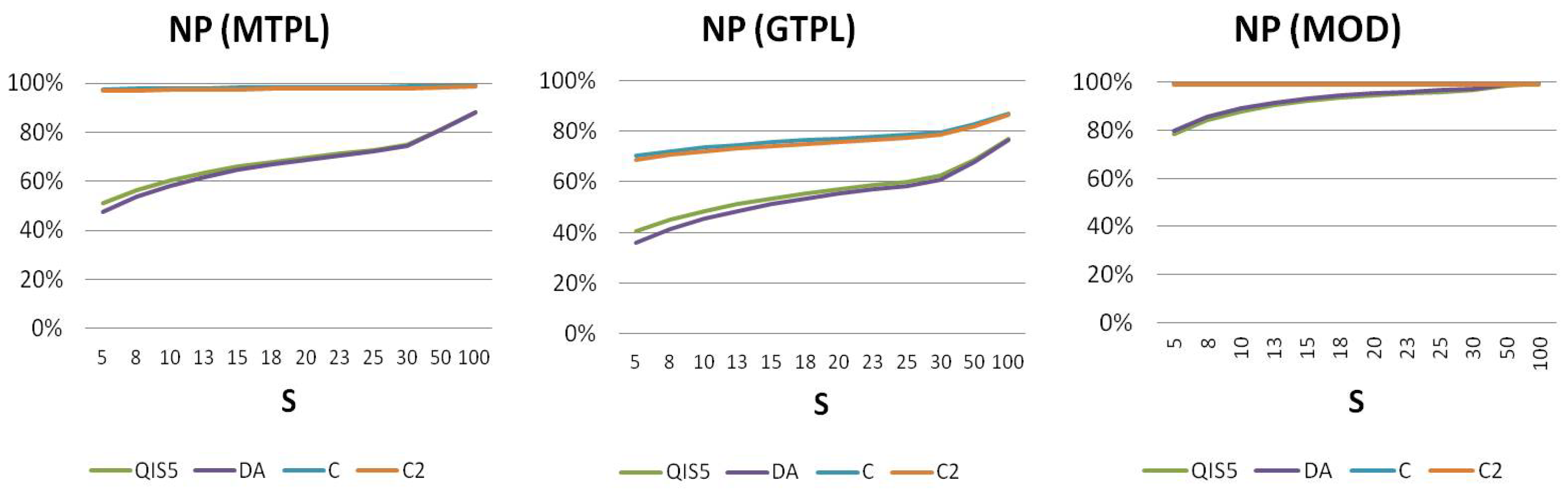
Figure 7.
Skewness of (gross or net) total losses under either lognormal distribution or collective risk model.
Figure 7.
Skewness of (gross or net) total losses under either lognormal distribution or collective risk model.

Table 1.
Premium and reserve volumes. Amounts in millions of euro.
| LoB | Next-Year Premiums | Best Estimate | Total | Weight on Total | ||
|---|---|---|---|---|---|---|
| MTPL | 544.76 | 725.93 | 1270.68 | 26.2% | 35.0% | 61.2% |
| GTPL | 133.17 | 570.42 | 703.60 | 6.4% | 27.5% | 33.9% |
| MOD | 79.15 | 22.60 | 101.76 | 3.8% | 1.1% | 4.9% |
| Total | 757.08 | 1318.95 | 2076.04 | 36.5% | 63.5% | 100.0% |
Table 2.
Parameters for premium risk.
| LoB | n | g | m | i | c | |||
|---|---|---|---|---|---|---|---|---|
| MTPL | 100,000 | 7% | 2% | 4000 | 6 | 3% | 5.0% | 14.0% |
| GTPL | 10,000 | 8% | 2% | 10,000 | 10 | 3% | −10.0% | 29.0% |
| MOD | 20,000 | 14% | 2% | 2500 | 2 | 3% | 10.0% | 27.0% |
Table 3.
according to different methodologies.
| LoB | ||||
|---|---|---|---|---|
| MTPL | 65.83% | 64.51% | 98.08% | 97.52% |
| GTPL | 53.37% | 51.09% | 75.49% | 74.10% |
| MOD | 92.21% | 93.24% | 99.93% | 99.02% |
© 2018 by the author. Licensee MDPI, Basel, Switzerland. This article is an open access article distributed under the terms and conditions of the Creative Commons Attribution (CC BY) license (http://creativecommons.org/licenses/by/4.0/).
Share and Cite
MDPI and ACS Style
Clemente, G.P. The Effect of Non-Proportional Reinsurance: A Revision of Solvency II Standard Formula. Risks 2018, 6, 50. https://doi.org/10.3390/risks6020050
AMA Style
Clemente GP. The Effect of Non-Proportional Reinsurance: A Revision of Solvency II Standard Formula. Risks. 2018; 6(2):50. https://doi.org/10.3390/risks6020050
Chicago/Turabian StyleClemente, Gian Paolo. 2018. "The Effect of Non-Proportional Reinsurance: A Revision of Solvency II Standard Formula" Risks 6, no. 2: 50. https://doi.org/10.3390/risks6020050
Note that from the first issue of 2016, this journal uses article numbers instead of page numbers. See further details here.