Bayesian Modelling, Monte Carlo Sampling and Capital Allocation of Insurance Risks

1
Department of Statistical Science, University College London, London WC1E 6BT, UK
2
Oxford-Man Institute, Oxford University, Oxford OX1 2JD, UK
3
System Risk Center, London School of Economics, London WC2A 2AE, UK
4
Fundação Getulio Vargas, Escola de Matemática Aplicada, Botafogo, RJ 22250-040, Brazil
5
RiskLab, Department of Mathematics, ETH Zurich, 8092 Zurich, Switzerland
*
Author to whom correspondence should be addressed.
Risks 2017, 5(4), 53; https://doi.org/10.3390/risks5040053
Submission received: 3 May 2017
/
Revised: 30 August 2017
/
Accepted: 31 August 2017
/
Published: 22 September 2017
(This article belongs to the Special Issue A Celebration of the Ties That Bind Us: Connections between Actuarial Science and Mathematical Finance)
Abstract
:The main objective of this work is to develop a detailed step-by-step guide to the development and application of a new class of efficient Monte Carlo methods to solve practically important problems faced by insurers under the new solvency regulations. In particular, a novel Monte Carlo method to calculate capital allocations for a general insurance company is developed, with a focus on coherent capital allocation that is compliant with the Swiss Solvency Test. The data used is based on the balance sheet of a representative stylized company. For each line of business in that company, allocations are calculated for the one-year risk with dependencies based on correlations given by the Swiss Solvency Test. Two different approaches for dealing with parameter uncertainty are discussed and simulation algorithms based on (pseudo-marginal) Sequential Monte Carlo algorithms are described and their efficiency is analysed.
1. Introduction
Due to the new risk based solvency regulations (such as the Swiss Solvency Test FINMA (2007) and Solvency II European Comission (2009)), insurance companies must perform two core calculations. The first one involves computing and setting aside the risk capital to ensure the company’s solvency and financial stability, and the second one is related to the capital allocation exercise. This exercise is a process of splitting the (economic or regulatory) capital amongst its various constituents, which could be different lines of business (LoBs), types of exposures, territories or even individual products in a portfolio of insurance policies. One of the reasons for performing such an exercise is to utilize the results for a risk-reward management tool to analyse profitability. The amount of capital (or risk) allocated to each LoB, for example, may assist the central management’s decision to further invest in or discontinue a business line.
In contrast to the quantitative risk assessment, where there is an unanimous view shared by regulators world-wide that it should be performed through the use of risk measures, such as the Value at Risk (VaR) or Expected Shortfall (ES), there is no consensus on how to perform capital allocation to sub-units. In this work we follow the Euler allocation principle (see, e.g., Tasche (1999) and (McNeil et al. 2010, sct. 6.3)), which is briefly revised in the next section. For other allocation principles we refer the reader to Dhaene et al. (2012).
Under the Euler principle the allocation for each one of the portfolio’s constituents can be calculated through an expectation conditional on a rare event. Even though, in general, these expectations are not available in closed form, some exceptions exist, such as the multivariate Gaussian model, first discussed in this context in Panjer (2001) and extended to the case of multivariate elliptical distributions in Landsman and Valdez (2003) and Dhaene et al. (2008); the multivariate gamma model of Furman and Landsman (2005); the combination of the Farlie-Gumbel-Morgenstern (FGM) copula and (mixtures of) exponential marginals from Bargès et al. (2009) or (mixtures of) Erlang marginals Cossette et al. (2013); and the multivariate Pareto-II from Asimit et al. (2013).
In this work we develop algorithms to calculate the marginal allocations for a generic model, which, invariably, leads to numerical approximations. Although simple Monte Carlo schemes (such as rejection sampling or importance sampling) are flexible enough to be used for a generic model, they can be shown to be computationally highly inefficient, as the majority of the samples do not satisfy the necessary conditioning event (which is a rare event). We build upon ideas developed in Targino et al. (2015) and propose an algorithm based on methods from Bayesian Statistics, namely a combination of Markov Chain Monte Carlo (for parameter estimation) and (pseudo-marginal) Sequential Monte Carlo (SMC) for the capital allocation.
As a side result of the allocation algorithm, we are able to efficiently compute both the company’s overall Value at Risk (VaR) and also its Expected Shortfall (ES), (partially) addressing one of the main concerns of Embrechts et al. (2014): For High Confidence Levels, e.g., and beyond, the “statistical quantity” VaR Can only Be Estimated with Considerable Statistical, as well as Model Uncertainty. Even though the issue of model uncertainty is not resolved, our algorithm can, at least, help to reduce the “statistical uncertainty”, measured by a variance reduction factor taking as basis a standard Monte Carlo simulation with comparable computational cost.
The proposed allocation procedure is described for a fictitious general insurance company with 9 LoBs (see Table 1 and Section 8). Further, within each LoB we also allocate the capital to the one-year reserve risk (due to claims from previous years) and the one-year premium risk.
In order to study the premium risk we follow the framework prescribed by the Swiss Solvency Test (SST) in (FINMA 2007, sct. 4.4). In this technical document, given company-specific quantities, the distribution of the premium risk is deterministically defined and no parameter uncertainty is involved. For the reserve risk, we use a fully Bayesian version of the gamma-gamma chain ladder model, analysed in Peters et al. (2017). As this model is described via a set of unknown parameters, two different approaches to capital allocation are proposed: a marginalized one, where the unknown parameters are marginalized prior to the allocation process and a conditional one, which is performed conditional on the unknown parameters and the parameter is integrated out numerically ex-poste.
The remainder of this paper is organized as follows. Section 2 formally describes marginal risk contributions (allocations) under the marginalized and conditional models. Section 3 reviews concepts of SMC algorithms and how they can be used to compute the quantities described in Section 2. We set the notation used for claims reserving in Section 4, before formally defining the models for the reserve risk (Section 5) and the premium risk (Section 6); these are merged together through a copula in Section 7. Section 8 and Section 9 provide details of the synthetic data used, the inferential procedure for the unknown parameters and the implementation of the SMC algorithms. Results and conclusions are presented, respectively, in Section 10 and Section 11.
2. Risk Allocation for the Swiss Solvency Test
In this section we follow the Euler allocation principle (see, e.g., Tasche (1999) and (McNeil et al. 2010, sct. 6.3)) and discuss how the risk capital that is held by an insurance company can be split into different risk triggers. As stochastic models for these risks involve a set of unknown parameters, we present an allocation procedure for a marginalized model (which arises when the parameter uncertainty is resolved beforehand) and a conditional model (which is still dependent on unknown parameters).
Although we postpone the construction of the specific claims payments model to Section 5 we now assume its behaviour is given by a Bayesian model depending on a generic parameter vector , for which a prior distribution is assigned. Probabilistic statements, such as the calculation of the risks allocated to each trigger, have to be made based on the available data, described by the filtration and formally defined in Section 4. This requirement implies that the uncertainty on the parameter values needs to be integrated out, in a process that must typically be performed numerically.
Therefore, to calculate the risk allocations we approximate the stochastic behaviour of functions of future observations, with the functions defined in Section 4. For the moment, let us denote by a multivariate function of , the future data, and the vector of model parameters. On the one hand, in the conditional model, we approximate the distribution of the components of the vector . On the other hand, in the marginalized model, the approximation is performed after the parameter uncertainty has been integrated out (i.e., marginalized). In this later framework, we approximate the distribution of the components of , where the random vector is defined as , with expectation taken with respect to . Note that, given , is a random variable, as it depends on future information, i.e., . Both in the conditional and in the marginalized models we use moment matching and log-normal distributions for the approximations and couple the distributions via a Gaussian copula.
Suppressing the dependence on the available information, , these two models (marginalized and conditional) are defined through their probability density functions (p.d.f.’s), and , respectively, which are both assumed to be combinations of log-normal distributions and a gaussian copula. For the conditional model, as we work in a Bayesian framework, the unknown parameter vector has a (posterior) distribution with p.d.f. . This is, then, combined with the likelihood to construct , the density used for inference under the conditional model.
For the methodology discussed in this work, the important features of these two models are that is known in closed form, whilst is not.
Remark 1.
As the “original” model for claims payments is a Bayesian model, we use the Bayesian nomenclature for both the marginalized and the conditional model. For the former, the Bayesian structure of prior and likelihood is hidden in Equation (1), as the parameter has already been marginalized (with respect to its posterior distribution). For the later, we explicitly make use of the posterior distribution of in Equation (2). Another strategy, followed in Wüthrich (2015), is to use an “empirical Bayes” approach, fixing the value of the unknown parameter vector , for example at its maximum likelihood estimator (MLE).
Under the marginalized model we define as the company’s overall risk. The SST requires the total capital to be calculated as the ES of S, given by
In turn, the Euler allocation principle states that the contribution of each component to the total capital in Equation (3) is given by
The allocations for the conditional model follows the same structure, with and S replaced, respectively, by and in Equation (4) and reads as
with . For the models discussed below the density of is not known in closed form, adding one more layer of complexity to the proposed method.
Remark 2.
Observe that the log-normal approximations are done at different stages in the marginalized and the conditional models. Therefore, we expect that the results will differ.
Although computing and is a static problem, for the sake of transforming the Monte Carlo estimation into an efficient computational framework, we embed the calculation of these quantities into a sequential procedure, where at each step we solve a simpler problem, through a relaxation of the rare-event conditioning constraint to a sequence of less extreme rare-events. In the next section we discuss the methodological Monte Carlo approach used to perform this task. The reader familiar with the concepts of Sequential Monte Carlo methods may skip Section 3.1.
3. SMC Samplers and Capital Allocation
For the marginalized and conditional models presented in Section 4 to Section 7 the marginal contributions in Equations (4)) and (5) cannot be calculated in analytic form for a generic model, so a simulation technique needs to be employed. In the sequel we provide a brief overview of a class of Monte Carlo methods, named Sequential Monte Carlo (SMC). For a recent survey in the topic, with focus on economics, finance and insurance applications the reader is referred to Creal (2012) and Del Moral et al. (2013). For a generic introductory review we refer the reader to Doucet and Johansen (2009).
3.1. A Brief Introduction to SMC Methods
The class of Sequential Monte Carlo (SMC) algorithms, also called Particle Filters, has its roots in the fields of engineering, probability and statistics where it was primarily used for sampling from a sequence of distributions (see, e.g., Gordon et al. (1993) and Del Moral (1996)). In the context of state-space models, SMC methods can be used to sequentially approximate the filtering distributions of non-linear and non-Gaussian state space models, solving the same problem as the Kalman filter—a technique with a long-standing tradition in actuarial mathematics (see, e.g., De Jong and Zehnwirth (1983) and Verrall (1989)).
The general context of a standard SMC method is that one wants to approximate a (often naturally occurring) sequence of p.d.f.’s with the support of each function in this sequence is given by , for , where t can be any artificial ordering of the sequence that is problem specific. We assume that is (only) known up to a normalizing constant, and we write
where .
3.1.1. SMC Algorithm
Procedurally, we initialize the algorithm sampling a set of N independent particles (as the samples are denoted in the literature) from the distribution and set normalized weights to , for all . If it is not possible to sample directly from , one should sample from an importance distribution and calculate its weights accordingly. Then the particles are sequentially propagated through each distribution in the sequence via three main processes: mutation, correction (incremental importance weighting) and resampling. In the first step (mutation) we propagate particles from time to time t, in the second one (correction) we calculate the new importance weights of the particles.
Without resampling, this method can be seen as a sequence of importance sampling (IS) steps, where the target distribution at each step t is (the unnormalized version of ) and the importance distribution is given by
where is the mechanism used to propagate particles from time to t, known as the mutation kernel. Therefore, after the mutation step each particle has (unnormalized) importance weight given by
These importance weights can be normalized to create a set of (normalized) weighted particles , with normalized weights . In this case, from the Law of Large Numbers,
–almost surely as , for any test function such that the expectation of under exists (see Geweke (1989)).
Remark 3.
The reader should note that the knowledge of up to a normalizing constant is sufficient for the implementation of a generic SMC algorithm, since the normalized weights are the same for both and .
In simple implementations of the SMC algorithm (such as the one discussed above), when the algorithmic time t increases, the estimates in Equation (8) become, eventually, effectively a function of one sample point ; what is observed, in practice, is that for some particle j, and for all the others the normalized weights are negligible. This degeneracy is measured using the Effective Sample Size (ESS) defined in Liu and Chen (1995) and Liu and Chen (1998) as
This quantity has the interpretation that is maximized when forms a uniform distribution on and minimized when for some j. One may also use the Gini index or the entropy as a degeneracy measure, as discussed, for example, in Martino et al. (2017).
One way to tackle this degeneracy problem is to unbiasedly resample the whole set of weighted particles, for example, choosing (with replacement) N samples from the system where each is selected with probability weight . In our algorithms we propose to resample the whole set of weighted samples whenever it is “too degenerate” and our degeneracy threshold is . Many different resampling schemes have been suggested in the literature and for a comparison between them we refer the reader to Douc and Cappé (2005) and Gandy and Lau (2015).
Although the resample step alleviates the degeneracy problem, its successive reapplication at each stage of the sampler produces the so-called sample impoverishment, where the number of distinct particles is extremely small. In Gilks and Berzuini (2001) it was proposed to add a “move” step with any kernel such that the target distribution is invariant with respect to it in order to rejuvenate the system. This kernel may be, for example, as a Markov Chain Monte Carlo (MCMC) kernel, which would begin with equally chosen weighted samples from the target distribution and then perturb them under a single step of a Metropolis Hastings acceptance-rejection mechanism. Note that in this case the samples start exactly in the target distribution’s stationary regime. Therefore, a single step of the Metropolis-Hastings accept-reject mutation is strictly valid and no burn-in is required.
More precisely, we can apply any kernel that leaves invariant to move the sample to (the hat denotes a sample after the resample step but before the “move” step), i.e.,
3.1.2. SMC Samplers
Although very general, the SMC algorithm presented above, in principle, requires the sequence of p.d.f.’s to have an increasing support. However it has been shown in Peters (2005) and Del Moral et al. (2006) that these algorithms can be applied to sequences of p.d.f.’s defined on the same support, leading to the so-called SMC sampler algorithm discussed below. This development is central for the insurance applications explored in this paper.
Given the sequence of densities (and its unnormalized version, ), where each element is defined over the same support, say , we create another sequence, defined on , the path space
which, for any Markov kernel is a density with as marginal (which can be seen by integrating out ). Note that, in Equation (9) time runs backwards, from t to 1. For completeness we define and
If is an IS density targeting then, see Equation (6),
is defined, for Markov kernels , as an IS density targeting . For we define .
As in the SMC algorithm, to generate a set of weighted samples from one can use a sequence of IS steps on the path space where the unnormalized importance weights are, at each time step , given by, see Equation (7),
where , for all . The normalized weights are then computed as
The pseudo-code of the SMC sampler procedure just described is found in Algorithm 1.
| Algorithm 1: SMC sampler algorithm. |
 |
The introduction of the sequence of kernels creates a new degree of freedom in the design of SMC samplers compared with the usual SMC algorithms, where only the forward mutation kernels should be designed. As discussed in Peters (2005) and Del Moral et al. (2006) if one wants to minimize the variance of the importance weights one strategy is to use the following approximation to the optimal backward kernel that minimizes the variance of the incremental weights (which cannot be computed in practice and must be approximated)
which leads to incremental weights
With the methodological tools provided by the SMC samplers we now proceed on how to adapt these methods to the allocation of risks under our generic marginalized and conditional models.
3.2. Allocations for the Marginalized Model
For a generic random vector with known marginal densities and distribution functions, respectively and , and copula density on , due to Sklar’s theorem (see Sklar (1959) and (McNeil et al. 2010, chp. 5)) the joint density of can be written as
where and . In order to approximate the marginal risk contributions from Equation (4) we can use samples from the distribution
where the set is defined, for , as
and the indicator function is one when and zero otherwise. It should be noted that since the boundary B in Equation (14) is given by with we have , see discussion on this point in Targino et al. (2015).
3.2.1. Reaching a Rare Event Using Intermediate Steps
Instead of directly targeting the conditional distribution the idea of the SMC sampler of Algorithm 1 is to sequentially sample from intermediate distributions with conditioning events that become rarer until the point we reach the distribution of interest (see Equation (14)). The benefit of such an approach is that the samples (particles) from a previous step (with a less rare conditioning event) are “guided” to the next algorithmic step (when targeting a rarer conditioning set) and, if carefully designed, no samples are wasted on the way to the target distribution, in the sense that no samples are incrementally weighted with a strictly zero weight. This “herds” the samples into the target sampling region of interest.
In order to sample from the target distribution defined in Equation (13) we use a sequence of intermediate distributions , such that and
with given by
Remark 4.
Differently from Targino et al. (2015), in order to make the algorithm more easily comparable with the one used for the conditional model, we do not transform the original random variable through its marginal distribution functions. Therefore, instead of sampling from the conditional copula we sample from the conditional joint distribution of .
The thresholds are chosen in order to have increasingly rarer conditioning events as a function of t, starting from the unconditional joint density. In other words, needs to satisfy . Note that the choice assumes , -a.s., otherwise . Depending on the choice of the thresholds it may be the case that the densities defined in Equation (15) are only known up to a normalizing constant so, from now on, we work with , the unnormalized version of :
If, at algorithmic time t, we have a set of N weighted samples from , with then we construct the following empirical approximation:
It should be noticed, though, that in our application the final threshold is not previously known. In these cases, an adaptive strategy, similar to the one studied in Cérou et al. (2012) can be implemented, where neither nor needs to be previously known. More details on this aspect of the algorithm are provided in Section 9.1.
3.3. Allocations for The Conditional Model
From the discussion in Section 2 we see that the main difference between the marginalized and conditional models is the fact that the former density is analytically known (in fact, it its approximated by an analytically known density) whilst the latter is defined through an integral of a known density, see Equations (1) and (2). In this section we discuss how to adapt the algorithm presented in Section 3.2 for situations where the target density cannot be analytically computed but a positive and unbiased estimator for it can be calculated.
Following the recent developments on pseudo-marginal methods (see Andrieu and Roberts (2009) and Finke (2015) for a survey in the topic) we substitute the unknown density in Equation (2) by a positive and unbiased estimate and show the SMC procedure still targets the correct distribution—a strategy similar to the ones proposed in Everitt et al. (2016) and McGree et al. (2015). In the context of rare event simulations a similar idea has been independently developed in Vergé et al. (2016) where the authors study the impact of the parameter uncertainty in the probability of the rare event, whilst we analyse the impact in expectations conditional to the rare event (as in Equation (5)).
The idea of replacing an unknown density by a positive and unbiased estimate is in the core of many recently proposed algorithms, such as the Particle Markov Chain Monte Carlo (PMCMC) of Andrieu et al. (2010), the Sequential Monte Carlo Squared (SMC) of Chopin et al. (2013) and Fulop and Li (2013) (see also the island particle filter of Vergé et al. (2015)) and the Importance Sampling Squared (IS) of Tran et al. (2014). In the context of Sequential Monte Carlo algorithms this argument first appeared as a brief note in Rousset and Doucet’s comments of Beskos et al. (2006), where it reads that “(...) a straightforward argument shows that it is not necessary to know [the weights] exactly. Only an unbiased positive estimate of is necessary to obtain asymptotically consistent SMC estimates under weak assumptions”.
To introduce the concept we first estimate by , which can be seen as a “one sample” approximation to the integral in Equation (2); then we show how to use an estimator based on samples from . These two approaches have been named in the literature (see Everitt et al. (2016) and references therein) as, respectively, the single auxiliary variable (SAV) and the multiple auxiliary variable (MAV) methods.
3.3.1. Single Auxiliary Variable Method
To avoid direct use of on the SMC sampler algorithm we provide a procedure on the joint space of and the parameter , defined as . The reader is referred to Finke (2015) for an extensive list of known algorithms which can also be interpreted in a extended space way. The target distribution on this new space is defined as the joint distribution of and and its marginal with respect to is precisely the density of the conditional model.
Formally, for , and we define
which has the desired marginal target distribution of interest:
Similarly to the densities defined in Equations (9) and (16) we define a sequence of target distributions both in and , respectively, as
and
where the second identity specifies the choices of , in terms of and .
Assuming we can perfectly sample from the distribution of (in our application this distribution is a posterior, from which samples are generated via simulation algorithms), to move samples backwards from time to s we split this process into sampling from (ignoring ) and then, conditional on , moving to . In other words, to sample
we split the process in two stages,
- ;
- .
The importance distribution on the path space of can be expressed as
and, once again, the second identity provides the choices of and , i.e.,
Therefore, a SMC procedure targeting the sequence produces unnormalized weights
that can be used to create weighted samples from , which is the desired marginal of , the density required for the capital allocation.
Remark 5.
From the structure of the mutation kernels it should be noticed that at each iteration t a new value of needs to be generated and used to sample . In other words, for each particle a different is to be used for each .
3.3.2. Multiple Auxiliary Variable
In the previous algorithm we, indirectly, estimate the density by . In this section we discuss how to use a different and more robust estimator, using samples from . In the context of pseudo-marginal Monte Carlo Markov Chain (MCMC) Andrieu and Vihola (2015) show that reducing the variance of the estimate of the unknown density leads to reduced asymptotic variance of estimators from the MCMC. For SMC algorithms this strategy has been used, for example, in McGree et al. (2015) and Everitt et al. (2016).
Before proceeding, we note that even in the case that the algorithm still produces asymptotic and unbiased estimators (when the number of particles ). However, the rate of variance reduction in the asymptotic estimates is directly affected by the choice of M (in a non-trivial manner). Furthermore, the asymptotic variance of Central Limit Theorem (CLT) estimators under the class of such pseudo-marginal Monte Carlo approaches is strictly ordered in M, with M increasing reducing the the asymptotic variance.
For any , a positive and unbiased estimate for can be constructed as
where and each is sampled independently from . Note that when only one sample of is used to estimate the estimator is reduced to . Also, note that point-wise when , by the law of large numbers. Indeed, since the random variable has density we obtain
Therefore the density constructed in Equation (18) is the marginal of the new target density defined on
Apart from the cumbersome notation, the same argument from the previous section can be used to show that a SMC procedure with estimated density replacing has unnormalized weights given by
when targeting a sequence with .
The algorithms described in this section contain several degrees of freedom, whose choices are discussed in detail in Section 9. In the next section we formally define the elements necessary for constructing the statistical models underlying the risk drivers and . We also present the formulas for the Solvency Capital Requirements (SCRs) under both the conditional and marginalized models.
After this brief introduction to SMC algorithms, in the following section we introduce the random variables used in the risk allocation process. In particular, we formally define the random vectors and discussed in Section 2, and identify its components with the one-year reserve risk and the one-year premium risk.
4. Swiss Solvency Test and Claims Development
For the rest of this work we assume all random variables are defined in the filtered probability space . We denote cumulative payments for accident year until development year (with ) on the LoB by . Moreover, in the ℓ-th LoB incremental payments for claims with accident year i and development year j are denoted by . Remark that these payments are made in accounting year .
The information (regarding claims payments) available at time for the ℓ-th LoB is assumed to be given by
and, similarly, the total information (regarding claims payments) available at time t is denoted as
Remark 6.
By a slight abuse of notation we also use and for the sigma-field generated by the corresponding sets. Note that for all , as we assume that contains not only information about claims payments, but also about premium and administrative costs.
The general aim now is to predict the future cumulative payments for at time t, given the information , in particular, the so-called ultimate claim . For more information we refer to Wüthrich (2015).
4.1. Conditional Predictive Model
As noted previously, we generically denote parameters in the Bayesian model for the ℓ LoB by . For the ease of exposition, whenever a quantity is defined conditional on it is going to be denoted with a bar on top of it.
At time , LoB ℓ and accident year predictors for the ultimate claim and the corresponding claims reserves are defined, respectively, as
Under modern solvency regulations, such as Solvency II European Comission (2009) and the Swiss Solvency Test FINMA (2007) an important variable to be analysed is the claims development result (CDR). For accident year , accounting year and LoB ℓ, the CDR is defined as
and an application of the tower property of the expectation shows that (subject to integrability)
Thus, the prediction process in Equation (21) is a martingale in t and we aim to study the volatility of these martingale innovations.
Equation (23) justifies the prediction of the CDR by zero and the uncertainty of this prediction can be assessed by the conditional mean squared error of prediction (msep):
Moreover, we denote the aggregated (over all accident years) CDR and the reserves, conditional on the knowledge of the parameter , respectively, by
Using this notation we also define the total prediction uncertainty incurred when predicting by zero as
Remark 7.
It should be remarked that, in general, as the parameter vector is unknown none of the quantities presented in this section can be directly calculated unless an explicit estimate for the parameter is used.
4.2. Marginalized Predictive Model
Even though cumulative claims models are defined conditional on unobserved parameter values, any quantity that has to be calculated based on these models should only depend on observable variables. Under the Bayesian paradigm, unknown quantities are modelled using a prior probability distribution reflecting prior beliefs about these parameters.
Analogously to Section 4.1 we define the marginalized (Bayesian) ultimate claim predictor and its reserves, respectively, as
We also define the marginalized CDR and notice, again using the tower property, that its mean is equal to zero
Furthermore, summing over all accident years i we follow Equation (26) and denote by and the aggregated version of the marginalized reserves and CDR, where the uncertainty in the later is measured via
4.3. Solvency Capital Requirement (SCR)
In this section we discuss how two important concepts in actuarial risk management, namely the technical result (TR) and the solvency capital requirement (SCR), can be defined for both the conditional and the marginalized models.
In this context the TR is calculated netting all income and expenses arising from the LoBs, while the SCR denotes the minimum capital required by the regulatory authorities in order to cover the company’s business risks. More precisely, the SCR for accounting year quantifies the risk of having a substantially distressed result at time , evaluated in light of the available information at time t.
As an important shorthand notation, we introduce three sets of random variables, representing the total claim amounts of the current year (CY) claims and of prior year (PY) claims, the later for both the conditional and marginalized models. These random variables are defined, respectively, as
In the standard SST model, CY claims do not depend on any unknown parameters and are split into small claims for the LoBs and into large events for the perils . Small claims are also called attritional claims and large claims can be individual large claims or catastrophic events, like earthquakes. In this context the company can choose thresholds such that claims larger than these amounts are classified as large claims in its respective LoBs.
To further simplify the notation we also group all the random variables related to the conditional and the marginalized models in two random vectors, defined as follows
Next we give more details on how the TR and the SCR are calculated in the generic structure of the conditional and the marginalized models.
4.3.1. SCR for the Conditional Model
At time the technical result (TR) of the ℓ-th LoB in accounting year based on the conditional model is defined as the following –measurable random variable:
where and are, respectively, the earned premium and the administrative costs of accounting year . For simplicity, we assume that these two quantities are known at time t, i.e., the premium and administrative costs of accounting year are assumed to be previsible and, hence, -measurable. Moreover, it should be noticed that in this context not only includes the claims payment information defined in Equation (20). The general sigma-field should be seen as a sigma-field generated by the inclusion in of the information about and , for .
Given the technical result for all the LoBs, the company’s overall TR based on the conditional model, and aggregated cost and premium are denoted, respectively, by
In order to cover the company’s risks over an horizon of one year, the Swiss Solvency Test is concerned with the 99% ES (in light of all the data up to time t):
where denotes the solvency capital requirement.
It is important to notice that even though the ES operator is being applied to a “conditional random variable”, namely , the operator is not being taken conditional on the knowledge of , otherwise this quantity would not be computable (as discussed in Remark 7). Instead, the SCR is calculated based on the marginalized version of the conditional model, where the parameter uncertainty is integrated out. More precisely, the expected shortfall is based on the following (usually intractable) distribution
In order to compute the SCR based on the conditional model we first discuss the measurablity of the terms in the conditional TR, which can be rewritten as
From the above equation we see the first two terms are, by assumption, measurable and so are all the terms of the form (payments already completed by time t), while the last summation is measurable and, therefore, a random variable at time t. Due to the dependence on the unknown parameter the conditional ultimate claim predictor is usually not measurable. However, under the special models introduced in Section 5 we have that depends only on the claims data up to time t and not on the unknown parameter vector, making it measurable. In this case one has
where, by assumption, is -measurable.
4.3.2. SCR for the Marginalized Model
As the parameter uncertainty is dealt with in a previous step, the calculation of the SCR for the marginalized model is simpler than its conditional counterpart.
Similarly to the conditional case, we define the TR for the marginalized model as
and its aggregated version as
Furthermore, the SCR for the marginalized model is given by
where in this case the expected shortfall is calculated with respect to the density .
Remark 8.
For the models discussed in Section 5, as does not depend on the parameter vector and we also have that .
Remark 9.
As we assume the cost of claims processing and assessment and premium are known at time t they do not differ from the conditional to the marginalized model.
5. Modelling of Individual LoBs PY Claims
For the modelling of the PY claims reserving risk we need to model or as given in Equation (29). The uncertainty in these random variables will be assessed by the conditional and marginalized mean square error of prediction (msep), introduced in Equations (25) and (28). In order to calculate the msep we must first expand our analysis to the study of the claims reserving uncertainty. To do so, in this section we present a fully Bayesian version of the gamma-gamma chain-ladder (CL) model, which has been studied in Peters et al. (2017).
Since in this section we present the model for individual LoBs, for notational simplicity we omit the upper index from all random variables and parameters.
Model Assumptions 1.
[Gamma-gamma Bayesian chain ladder model] We make the following assumptions:
- (a)
- Conditionally, given and , cumulative claims are independent (in accident year i) Markov processes (in development year j) withfor all and .
- (b)
- The parameter vectors and are independent.
- (c)
- For given hyper-parameters the components of are independent such thatfor , where the limit infers that they are eventually distributed from an improper uninfomative prior.
- (d)
- The components of are independent and -distributed, having support in for given constants for all .
- (e)
- , and are independent and , for all .
In Model Assumptions 1 (c) the (improper) prior distribution for should be seen as a non-informative limit when of the (proper) prior assumption
The limit in (c) does not lead to a proper probabilistic model for the prior distribution, however, based on “reasonable” observations the posterior model can be shown to be well defined (see Equation (38)), a result that has been proved using the dominated convergence theorem in Peters et al. (2017).
From Model Assumptions 1 (a), conditional on a specific value of the parameter vectors and , we have that
which provides a stochastic formulation of the classical CL model of Mack (1993).
Even though the prior is assumed improper and does not integrate to one, the conditional posterior for is proper and, in addition, also gamma distributed (see Appendix A and (Merz and Wüthrich 2015, Lemma 3.2)). More precisely, we have that
with the following parameters
Therefore, given this model belongs to the family of Bayesian models with conjugate priors that allows for closed form (conditional) posteriors – for details see Wüthrich (2015).
The marginal posterior distribution of the elements of the vector is given by
with and defined in Equation (37). We note that as long as Model Assumptions 1 (d) and the conditions in Lemma A1 are satisfied, then one can ensure the posterior distribution of is proper.
Therefore, under Model Assumptions 1 inference for all the unknown parameters can be performed. It should be noticed, though, that differently from the (conditional) posteriors for Equation (36), the posterior for Equation (38) is not recognized as a known distribution. Thus, whenever expectations with respect to the distribution of need to be calculated one needs to make use of numerical procedures, such as numerical integration or Markov Chain Monte Carlo (MCMC) methods.
5.1. MSEP Results Conditional on
Following Model Assumptions 1 we now discuss how to explicitly calculate the quantities introduced in Section 4. We start with the equivalent of the classic CL factor. From the model structure in Equation (35) we define the posterior Bayesian CL factors, given , as
which, using the gamma distribution from Equation (36), takes the form
i.e., is identical to the classic CL factor estimate.
Following Equation (21) we define the conditional ultimate claim predictor
which can be shown (see (Wüthrich 2015, Theorem 9.5)) to be equal to
where this is exactly the classic chain ladder predictor of Mack (1993). For this reason we may take Model Assumptions 1 as a distributional model for the classical CL method. Additionally, the conditional reserves defined in Equation (21) and Equation (26) are also the same as the classic CL ones, that is,
The importance of Equation (40) relies on the fact that it does not depend on the parameter vector . In other words, the ultimate claim predictor based on the Bayesian model from Model Assumptions 1 conditional on – which is, in general, a random variable – is a real number (independent of ). This justifies the argument used on the calculation of Equation (32).
Remark 10.
Using the notation from the previous sections the parameter vector plays the role of as the only unknown, since, due to conjugacy properties, can be marginalized analytically.
For the Bayesian model from Model Assumptions 1 the msep conditional on has been derived in (Wüthrich 2015, Theorem 9.16) as follows, for
where
Moreover, the conditional msep has been shown to be finite if, and only if, . We also refer to Remark 12, below.
The aggregated conditional msep for is also derived in (Wüthrich 2015, Theorem 9.16), and given by
Remark 11.
The assumption that is made in order to guarantee the conditional msep is finite and we enforce this assumption to hold for all the examples presented in this work. See also Remark 12, below.
5.2. Marginalized MSEP Results
The results in the previous section are based on derivations presented in Merz and Wüthrich (2015) and Wüthrich (2015) where the parameter vector is assumed to be known. In this section we study the impact of the uncertainty in over the mean and variance of in light of Model Assumptions 1, which can be seen as a fully Bayesian version of the models previously mentioned.
In order to have well defined posterior distributions for , through this section we follow Lemma A1 and assume that, for all development years and , we have or at least one accident year is such that . For all the numerical results presented this assumption is satisfied.
Lemma 1.
The ultimate claim estimator under the marginalized model is equal to the classic chain ladder predictor, i.e., .
Proof.
Proposition 1.
The msep in the marginalized model is equal to the posterior expectation of the msep in the conditional model, i.e.,
Proof.
From the law of total variance we have that
and the last equality follows from Lemma 1 and the fact that is independent of . ☐
Remark 12.
Following the conditions required for finiteness of the conditional msep, in the unconditional case, one can see that whenever . Furthermore, we note that this condition can be controlled during the model specification, i.e., the range of the is chosen such that all posteriors are well-defined.
5.3. Statistical Model of PY Risk in the SST
Note that the distributional models derived in Section 5.1 and Section 5.2 are rather complex. To maintain some degree of tractability, the overall PY uncertainty distribution is usually approximated by a log-normal distribution via a moment matching procedure.
5.3.1. Conditional PY Model
As discussed in Section 4.3, when modelling the risk of PY claims we work with the random variables , defined in Equation (29). Due to their relationship with the conditional CDR, see Equations (22) and (23) and the results discussed in Section 5.1, we can use the derived properties of these random variables to construct the model being used for .
The conditional mean (see Equations (22), (23) and (41)) and variance (see Equations (25) and (44)) of the random variable are as follows
Given mean and variance, we make the following approximation, also proposed in the Swiss Solvency Test (see (FINMA 2007, sct. 4.4.10)).
Model Assumptions 2
(Conditional log-normal approximation). We assume that
with and .
Although the distribution of under Model Assumptions 1 can not be described analytically it is simple to simulate from it. To test the approximation of Model Assumptions 2 we simulate its distribution under the gamma-gamma Bayesian CL model (with fixed ) and compare it against the log-normal approximation proposed. For the hyper-parameters presented in Table 2 (and calculated in Section 8) the quantile-quantile plot of the approximation is presented in Figure 1. For all the LoBs we see that the log-normal distribution is a sensible approximation to the original model assumptions. Note that although the parameters used for the comparison are based on the marginalized model Figure 5 and Figure 6 show that they are “representative” values for the distributions of and .
5.3.2. Marginalized PY Model
As an alternative to the conditional Model Assumptions 2 we use the moments of calculated in Lemma 1 and Proposition 1 and then approximate its distribution. Note that due to the intractability of the distribution of the variance term defined in Equation (45) can only be calculated numerically, for example, via MCMC.
Model Assumptions 3
(Marginalized log-normal approximation). We assume that
with and .
The same comparison based on the quantile-quantile plot of Figure 1 can be performed for the marginalized model and the results are presented in Figure 2. Once again, the log-normal model presents a viable alternative to the originally postulated gamma-gamma Bayesian CL model, even though for Motor Hull, Property and Others the right tail of the log-normal distribution is slightly heavier.
6. Modelling of Individual LoBs CY Claims
Model Assumptions 1 do not assume any specific distribution for , the CY claims. These claims are treated differently in the Swiss Solvency Test from PY claims and the models used for these claims are explained in Section 6.1 and Section 6.2, below. Throughout this section, we denote by the expected number of CY claims over the next year, which is the sum of the expected CY small claims and the expected CY large claims .
6.1. Modelling of Small CY Claims
As mentioned in the SST Technical Document (FINMA 2007, sct. 4.4.7), the SST does not make any explicit assumption about the distribution of individual claims; instead, the annual claims expenses are only represented with their expected value and variance. More precisely, in (FINMA 2007, sct. 8.4.5.2) the distribution of the premium risk, is assumed to be such that
where the constants and are provided by the regulatory authority (under the names of parameter uncertainty and random fluctuation, respectively). Their values for the 2015 solvency test are found in FINMA (2016). In order to fully specify the model for CY small claims one also needs to decide on the mean of the variable , but we postpone a detailed discussion on this point until Section 8.2, where we also present the value of .
Model Assumptions 4
(Distribution of CY small claims). For known constants and we set
with and
6.2. Modelling of Large CY Claims
In the SST (see (FINMA 2007, sct. 4.4.8)), large CY claims are split into two groups. The first group of large claims are those triggered by the same market-wide event (a hailstorm, for example) and with many simultaneous (small) claims. These types of claims are likely to affect all market participants and are called “cumulated claims”. The second group encompasses individual claims with a large claim amount, which includes, as exemplified in (FINMA 2007, sct. 4.4.8), fire in a factory building.
For each risk trigger, CY large claims are required to be modelled as a compound Poisson random variable with i.i.d. Pareto severities, i.e.,
where is the number of large claims in LoB under consideration and model the intensity of large claims. Here we denote by a random variable with density for . It is assumed in the SST that large claims are i.i.d. within the same risk trigger and also between different risk triggers, and independent of all and .
As a notational remark, if Z follows a Compound Poisson – Pareto model as a shorthand notation we write , with the same parameter interpretation as in Equation (49).
6.2.1. SST Model for Cumulated Claims
In this section we discuss the modelling of cumulated claims (those triggered by a market-wide event) which are modelled as an event that impacts the whole market and then scales down to an individual insurance company through its market share. In particular, we present the modelling approach used in (1) Motor Hull LoB due to hail events and (2) Workers Compensation (UVG) LoB due to a market-wide large accident.
In both cases market-wide parameters for a compound Poisson model with Pareto intensities have been determined by the regulator, (based on a large claims data set). The aggregated market-wide loss is given by
where denotes a compound distribution with frequency given by and severity given by . The corresponding market-wide parameter values are found in FINMA (2016).
Denoting by the company’s threshold after which losses are classified as large and m its market share in the ℓ-th LoB, to be consistent with its assumption the company should model market-wide large events as events above the threshold of
Then, the market-wide total loss (viewed from the specific company in consideration) is defined as
from which it is easy to see that the only unknown parameter is , since in the SST the Pareto parameter is kept the same. This frequency parameter is chosen such that the company’s view of the market-wide events is equivalent to the suggested market-wide process. In other words, hence
Therefore, from the company’s point of view, its own large claims are modelled as
Following the SST Technical Document FINMA (2007), an upper bound (provided by the regulator) is included in each Pareto random variable within the random sum. In other words, the final distribution of the company’s large cumulated claims is given by
where , a Pareto distribution defined in with tail index .
For efficiency purposes, this distribution is approximated by a single Pareto, with the same mean. This leads us to the following model assumptions.
Model Assumptions 5
Remark 13.
The reader should note that for large CY claims no parameter uncertainty is considered, since both , and γ are given by the regulator, the market share, m can be perfectly calculated and β is chosen by the company.
6.2.2. SST Model for Individual Claims
For individual large events, the SST provides , the probability of observing losses larger than CHF 1 million and standard values for , for and (see Table FINMA (2016)). Since the probability of large claims provided by the SST is based on a lower threshold of CHF 1 million, a thinning process of the CP-P has to be done if the company decides to use .
Following the same procedure presented in Section 6.2.1 we can see that the company’s large individual claims are modelled as
with an expected number of claims larger than equal to
where denotes the expected total number of CY claims in the ℓ-th LoB. Similarly, the regulator also requires a upper bound in the Pareto random variables, leading to the following distribution of large losses
As in Section 6.2.1, the distribution of is approximated by a single Pareto, with the same mean and Pareto index .
7. Joint Distribution of PY and CY Claims
Although the SST does not assume any parametric form for the joint distribution of or (defined in Equations (30) and (31), respectively) it is required that a pre-specified correlation matrix is used (see FINMA (2016)). In this section we discuss how to use the conditional and marginalized models to define a joint distribution satisfying this correlation assumption.
It is important to notice, though, that the SST correlation matrix may not be attainable for some joint distributions, as discussed in Appendix B in the case of log-normal marginals (in Devroye and Letac (2015) the authors discuss a similar problem). Let us denote by the set of all , symmetric, positive semi-definite matrices with diagonal terms equal to 1; and by the correlation matrix of a random vector , with elements . The question asked in Devroye and Letac (2015) is: given , does there exist a copula C such that ? The answer is yes, if and the authors postulate that for there exists such that there is no copula C such that .
It should be noted that, since in the SST the CY large claims are assumed to be independent from all the other risks, the correlation matrix of is essentially a correlation matrix between and the same is true also for the conditional model.
Regardless of assuming a conditional or a marginalized model, SST’s correlation matrix should be such that, for (recall that L are the number of LoBs and P the number of perils),
Remark 14.
In the conditional model we need to “integrate out” the parameter uncertainty, otherwise the (conditional) correlation would be dependent on an unknown parameter and could not be matched with the numbers provided by the SST.
7.1. Conditional Joint Model
Under Model Assumptions 2, 4, 5 and 6 our interest lies on modelling the joint behaviour of the vector . Under Model Assumptions 1 it can be shown that the required conditional independence between and given is equivalent to the conditional independence between and given and .
Moreover, since all the marginal conditional distributions of the prior year claims and small current year claims are assumed to be log-normal, following Equations (30) and (31), the notation can be further simplified to
with , and defined in Model Assumptions 2 and 4. For example, for , , defined in Model Assumptions 4.
We are now ready to define the joint conditional model to be used.
Model Assumptions 7
(Conditional joint model). Based on Model Assumptions 2 and 4 we link the marginals of the conditional model through a Gaussian copula with correlation matrix , with elements . More formally, given and the joint distribution of is given by
where denotes the conditional distribution of defined in Equation (52) and is the Gaussian copula with correlation matrix denoted by .
Remark 15.
In this section the parameter matrix should be understood as a deterministic variable, differently from and . For this reason we do not include it on the right hand side of the conditioning bar. Instead, whenever needs to be explicitly written, we include it on the left hand side of the bar, separated by the function (or functional, for expectations) arguments by a semicolon.
In order to match SST’s correlation matrix , under Model Assumptions 1 and 4, the following equation needs to be solved with respect to :
To compute the right hand side of the equation above we first notice that
where, from Equation (46) and the discussion in Section 6.1,
and from Equation (A3), Appendix B,
Therefore, to satisfy Equation (53) needs to be chosen such that the following implicit relationship (which can be solved through any univariate root search algorithm) holds:
7.2. Marginalized Joint Model
Similarly to Section 7.1, in this section we will fully characterize the joint distribution of under Model Assumptions 3, 4, 5 and 6.
From these assumptions we define the following notation:
Model Assumptions 8
(Marginalized joint model). Based on Model Assumptions 3 and 4 we link the marginal distributions of the marginalized model through a Gaussian copula with correlation matrix , with elements . More formally, given the joint distribution of is given by
where denotes the conditional distribution of defined in (Equation 54) and is the Gaussian copula with correlation matrix .
In order to match SST’s correlation matrix, in the joint marginalized model the Gaussian copula correlation is chosen such that (see Equation (A4), Appendix B) it satisfies
8. Data Description and Parameter Estimation
In this section we discuss how we set up the parameters in the models discussed so far, starting from the balance sheet of a fictitious insurance company. Using this balance sheet and the information contained in the SST we generate realistic claims triangles (see Appendix C) and, based on them, we show how to perform Bayesian inference for the unknown parameters. Our starting point is the fictitious balance sheet shown in Table 1, which is intended to represent a large insurance company in Switzerland (for this reason all monetary units should be understood as millions of Swiss Francs (CHF)).
8.1. Hyperparameters for
Based on SST’s standard runoff pattern (see Table 3) we first compute the implied CL factors as follows (once again we suppress the index ℓ of the LoB). If is the deterministic cumulative claims payment pattern for development year j we define
These values can, then, be used as a hyperparameter in the prior for (see Model Assumptions 1, item (c)).
To generate data from the model (see Appendix C) we fix and , where is Mack’s standard deviation estimate calculated from exogenous triangles. The values of are presented in Table 4. That is, should be understood as a (deterministic) prior payment pattern.
8.2. Current Year Small and Large Claims
To calculate the expected number of CY claims, , defined in Section 6, we first set our prior belief for the claims ratio for each LoB, i.e., how much of the premium in that LoB is used to cover incoming claims (all the rest covers business’ costs). This information is available in Table 5, along with the average claim amount. Based on these values the expected number of claims is defined as
Given the expected number of CY claims, , this value is used to compute the expected number of individual large claims, , as in Equation (51). Using the fact that we calculate the coefficient of variation for small CY claims as given in Equation (48).
The last ingredient in Model Assumptions 4 is which is given by
and the expectation on the right hand side is given either in Model Assumptions 5 or Model Assumptions 6, depending on the LoB.
For the large claims from Model Assumptions 5 and 6 we assume the threshold for large claims to be equal to 5 (millions of CHF). For the large cumulated claims we use LoBs market share as given in Table 5. The resulting parameters can be found in Table 2. Note these parameters are the same both for the marginalized and conditional models.
8.3. Parameter Estimation
In this section we discuss how to compute the posterior distributions of the variance parameters in Model Assumptions 1, which are used to compute quantities such as the marginalized msep from Section 5.2.
In order to compute the posteriors of , we assume priors centred at Mack’s Mack (1993) CL standard deviation estimator normalized by the CL factor f, both implied by the data. Formally,
where
To generate samples from the posteriors we use a Metropolis-Hastings algorithm, with proposals given by a truncated Normal centred at the current point and standard deviation equal to . All the chains are started at the CL variance estimate and the upper limit for the prior, is set as times the CL variance estimate. To be left with samples from the posterior we ran the Markov chains for 12,500 iterations, discarding the first as a burn-in and keeping every 10th iteration of the remaining simulations.
Some of the results are presented in Figure 3 where one finds the unnormalized posteriors, the histogram of the MCMC outputs and a red dashed line indicating the CL variance estimate for three different LoBs: (a) MTPL, (b) Motor Hull and (c) Property. As expected, for unidimensional and unimodal densities the resulting estimates are highly accurate. It is also worth noticing that the larger the development year j the more diffuse the posterior is, due to the diminishing amount of data available. In the limit, when the information available is not enough to estimate the variance parameter and, therefore, as can be seen from the posterior distribution derived in Equation (38), the posterior is the same as the prior.
Using the sample of size mentioned above, the calculated parameters for the marginalized model are presented in Table 2. For the conditional model we use the same sample from the posterior and calculate the one value of and for each sampled value . The resulting (transformed) samples are presented as histograms in Figure 5 and Figure 6 and, for comparison only, the relevant marginalized parameters are included as a red dashed line.
8.4. The Correlation Matrices
For the copula correlation matrices we follow the procedures outlined in Section 7.1 and Section 7.2. The resulting matrix for the marginalized model is found in Table 6. From FINMA (2016) it can be seen the values in are very similar to ones in the standard . Also, it worth noticing that differently from SST’s original correlation matrix, the block is no longer symmetric, i.e., in order to have the term of the matrix is not equal to the term of the same matrix.
The results for the copula correlation follow the same patterns as and for this reason its values are omitted.
9. Details of the SMC Algorithm
9.1. Selection of Intermediate Sets
Recall that a key component of the proposed SMC Sampler solution is to create a relaxation of the rare-conditional events that constrain the target posterior into a sequence of increasingly difficult constraints. In this section we discuss how one can select the sequence of constraint relaxations in an adaptive manner.
For both the marginalized and the conditional models we use an adaptive strategy similar to Cérou et al. (2012) in order to select adaptively online (as the algorithm runs) the levels , as well as the total number of intermediate sets T. When levels are being chosen adaptively one of the main advantages of the proposed SMC algorithm is the ability to estimate, in one run, the company-wide value at risk, the expected shortfall as well as the risk allocations.
Starting from (or if the conditional model is being used) the idea consists of, at each algorithmic iteration , choosing the next level, , such that a percentage of the –particles is above this set. More formally, we set to be the empirical quantile of the weighted sample or , where and denote, respectively, the sum of the components of and . Therefore, at algorithmic time t the level corresponds to an estimate of the -th quantile of the target distribution. In our examples we set which induces intermediate quantiles seen in Table 10 for the algorithm. Note that, given a value of the number of levels in the algorithm is deterministic. For example, for there are 7 levels until the estimated quantile is above .
An alternative approach to choosing the level sets is to use the classic normalizing constant estimator derived from the SMC sampler algorithm (see (Del Moral et al. 2006, sct. 3.2.1)). Using the notation from Section 3 we have that the normalizing constant can be estimated as
where and are, respectively the normalized and the incremental weights at time .
Similarly to our proposed estimate, in this alternative route one would choose such that of the time particles are above this level. Using the estimator in Equation (56) one could stop the algorithm as soon as . The main disadvantage of this approach is that although can be proven to be unbiased and asymptotically normally distributed when the number of particles (see (Del Moral 2004, Propositions 7.4.1 and 9.4.1) and Pitt et al. (2012) for a proof in the special case of state-space models) one can not guarantee . In our experiments the results based on this classic estimate were deemed unsatisfactory, as we observed estimates of the normalizing constant as large as 15, as finite sample realizations.
9.2. Marginalized Model
9.2.1. The Forward Kernel
Similarly to (Targino et al. 2015, sct. 6.1) we propose a mutation kernel such that the condition is always satisfied. Due to the independence assumption of the CY large claims (the P Pareto variables) we first independently mutate the Pareto coordinates, following their true (unconditional) marginal and then mutate the other variables.
First we split the vector into its log-normal and Pareto components, , where and . Using this notation and denoting the vector without its m-th component, we use
where the kernel , which mutates all but the m-th dimension of , consists of independent moves in each dimension, i.e.,
Note that these moves are also independent of the P Pareto mutations.
Let us denote the weighted sample approximating
as defined in Equation (15). The components of the mutation kernel are then defined as
where and are the empirical mean and variance of when
For the mutation of the remaining dimension, m, to ensure all the samples satisfy the condition we proceed as follows. First we define
and then sample the last component according to
where denotes the density of a Normal distribution with mean and variance truncated on support .
9.2.2. The Backward Kernel
For the backward kernel we follow the discussion in Section 3.1.2 and use the (approximation to the) optimum kernel of Del Moral et al. (2006), given by equation Equation (11)
where denotes the unnormalized weights at time t and the weighted sample targets the unnormalized density . Proceeding in this way the unnormalized weights for the SMC sampler algorithm (see Algorithm 1) satisfy the following recursion
9.2.3. The MCMC Move Kernel
To improve particle diversity after a resampling step (which is performed whenever the effective sample size drops bellow ) the following MCMC move kernel is applied to the particles.
As in (Targino et al. 2015, sct. 6.2) we propose a Gibbs-type update combined with a slice sampler (see Neal (2003)). For notational simplicity we suppress the dependence in t in the vector and denote the vector where the first m components have already been updated in the Gibbs scan. The full conditional for the m-th component of is given by
which is can be sampled from using an unidimensional slice sampler (see Neal (2003)).
9.3. Conditional Model
Following the discussion in Section 3.3.2 we use equation Equation (19) as an approximation to the unknown density . For our simulations samples of the unknown parameter are used, where
and each vector contains all the unknown variance parameters for the ℓ-th LoB. Therefore, and it should be noticed the superscript have a different interpretation from those in .
As the parameter estimation step described in Section 8.3 is independent of the allocation process we assume samples for each unknown parameter vector have already been created. Therefore, to sample we first sample an index and then .
9.3.1. The Forward Kernel
The forward kernel used for the conditional model follows the same structure as the one used in the marginalized model and described in Section 9.2.1: first we sample the P independent Pareto variables (with the same distribution as in the marginalized case) and then the remaining variables. More precisely,
where the last term is defined in equation Equation (57) and and are now the empirical mean and variance of . Likewise,
with the last term defined in equation Equation (58). As samples from have already been generated through MCMC then the mutation kernel in the extended space, , is completely characterized.
9.3.2. The Backward Kernel
As in Section 9.2.2 we use the optimum backward kernel in the extended space , which for the conditional model leads to the following incremental weights (see Equation (12))
9.3.3. The MCMC Move Kernel
The MCMC move kernel used for the conditional model needs to keep the target distribution in the extended space, , invariant. The strategy adopted is to first sample and then .
For the second step above we use exactly the same Gibbs-sampler update as in Section 9.2.3, with replaced by .
10. Results
In this section we present the results of the SMC procedure when used to calculate the expected shortfall allocations from Equations (4) and (5) of the solvency capital requirement.
Before proceeding to the results calculated via the SMC algorithm, in order to understand the simulated data presented in Figure 4, in Table 2 we present some results based on a “brute force” Monte Carlo (rejection-sampling) simulation, which is taken as the base line for comparisons with the SMC algorithm. The table is divided in three blocks of rows, with PY claims, CY small (CY,s) claims and CY large (CY,l) claims.
First of all, it should be noticed that the reserves presented on the first block of Table 2 are the ones implied by the data, which we then assume to be the true ones (ignoring, from now on, the initial synthetic data from Table 1). That is, based on initial parameters we have generated synthetic claims development triangles, which naturally deviate slightly from their expected values. The parameters and for PY claims are related to the marginalized model (for the parameters of the conditional model see Figure 5 and Figure 6). It is also important to note that only the PY parameters are different between the conditional and marginalized models.
For each LoB the standalone expected shortfall (ES) is calculated analytically and its value is, then, combined with the LoB’s expectation to calculate the solvency capital requirement (SCR). These values are added up, both within risk type (i.e., PY, CY,s and CY,l) and globally, in order to calculate the overall standalone capital. For the marginalized and conditional models the columns “ES” and “SCR” denote, respectively, the expected shortfall and capital allocations to each LoB. These values are compared to their standalone counterparts to generate the diversification benefit, which is around 45% for PY and CY,s claims (regardless of the model used) and ranges between 30% and 70% within the PY and CY,s groups. Due to the independence assumptions the largest diversification benefit comes from the CY,l claims, where the capital is reduced by around 95%.
The data presented in Table 2 is calculated as follows. For the marginalized model (and conditional model in brackets), () independent samples of the model are generated in order to calculate the overall . Conditional on this value, for each LoB we then generate () samples above the VaR and use the average of these samples as the true ES allocation (presented in Table 2). In order to asses the variance of the estimators, we divide these samples into groups of ( for the conditional model) simulations. More formally, we approximate the ES allocations , defined in Equation (4), by
where stands for the estimate (using particles) from the k-th run (out of ), which is defined according to
Similarly to the analysis performed in Peters et al. (2017) the impact of the prior density can be assessed by comparing the sum of the SCR allocations with the SCR from the “empirical Bayes model”, i.e., the model where the prior for is set as a Dirac mass on , see Equation (55). In this case we have that the total capital is equal to SCR = 505.48 and the fully Bayesian model with prior defined with (see Section 8.3) requires more capital (both in the marginalized and conditional cases).
To check the accuracy of the SMC procedure we first analyse the estimate of the level sets (intermediate VaRs). For , Figure 7 and Figure 8 show, respectively, the histogram of the levels (as per Table 10) for the marginalized and conditional models. The red dashed bars represent the true value of the quantiles (based on the “brute force” MC simulations), which is very close to the mode of the empirical distribution of the SMC estimates. It should be noticed, though, that the SMC estimates seem to be negatively biased and the bias appears to become more pronounced for extreme quantiles. Apart from this negligible bias we assume the levels are being sensibly estimated and proceed, as in Targino et al. (2015), to calculate the relative bias and the variance reduction of the SMC method when compared to a MC procedure.
For each of the LoBs the plots on the Figure 9 and Figure 10 show the relative bias, defined as
where is computed analogously to the MC estimate but, instead, using the SMC method, with . The behaviour of the two models is very similar, and we observe that the bias in the PY and CY,s allocations are negligible (less than 5%) while for some of the large CY risks a higher bias (of more than 10%) may be observed. Apart from the difficulty of performing the estimation based on Pareto distributions we stress the fact that although these errors may look large, as we can see from Table 2, their impact in the overall capital are almost imperceptible, due to the small capital charge due to these risks.
Another way to compare the SMC calculations is through the actual capital charges, as seen in Figure 11. In this figure we compare the SCR calculated via the MC scheme discussed above with the SMC results for the quantile level right before (which, for is ) and the one right after it (). From this figure we see the SMC calculation based on the quantile is very precise, for both the marginalized and conditional models. Visually, the only perceivable difference comes from the CY,l claims, which accounts (in total) for less than of the overall capital.
To calculate the improvement generated by the SMC algorithm compared to the MC procedure we need to analyse the variance of the estimates generated by both methods, under similar computational budgets.
We start by noticing that the expected number of samples in the Monte Carlo scheme in order to have samples satisfying the condition is equal to , which can be prohibitive if is very close to 1. Then, similarly to Equation (59) we define the empirical variance of the MC and the SMC algorithms which are, then, compared as follows
The variance reduction statistics defined in Equation (60) takes into account how many samples one needs to use in order to generate samples via rejection sampling or using the SMC algorithm. The later also takes into account the fact that T levels are being used and in each one samples need to be generated. For the conditional model we further multiply the denominator by the number of samples used to estimate the unknown density, which in our examples is set to .
The results follow on Figure 12 and Figure 13. As in Targino et al. (2015) we observe that the variance of the SMC estimates become smaller (compared to the MC results) for larger quantiles. In particular, for the quantiles of interest the variance of the marginal ES allocation estimates are around times smaller than its MC counterparts, while the overall ES estimate is slightly less variable for the MC scheme.
For the marginalized model we also present two plots in Figure 14, related, respectively, to the sensitivity to (a) the parameter and (b) the number of samples, . In Figure 14a, for the same number of samples, we analyse the bias relative to the ES allocations of the first quantile larger than (top plot) and the previous one (bottom plot) for . The quantiles used in these different setups are presented in Table 10. Although the results may look slightly different, the main message is the same: the “higher” quantile is effectively unbiased for PY and CY,s risks but presents a negative bias of around for some of the CY,l risks.
Regarding the sensitivity to the number of particles in the SMC algorithm, as expected, the absolute bias decreases when the number of samples increases, as seen in Figure 14b. Although the SMC algorithm is generically guaranteed to be unbiased when the trade-off between bias and the variance reduction in the allocation problem may lead us to accept a small bias in order to have a smaller variance.
11. Conclusions
In this paper we provide a complete and self-contained view of the capital allocation process for general insurance companies. As prescribed by the Swiss Solvency Test we break down the company’s overall Solvency Capital Requirement (SCR) into the one-year reserve risk, due to claims from previous years (PY) and the one-year premium risk due to claims’ payments in the current year (CY). The later is further split into the risk of normal/small claims (CY,s) and large claims (CY,l). For the premium risk in each line of business we assume a log-normal distribution for CY,s risks with mean and variance as per the SST, which also describe a distribution for CY,l risks, in this case Pareto. For the reserve risk, as in Peters et al. (2017), we postulate a Bayesian gamma-gamma model which, for allocation purposes, is approximated by log-normal distributions leading to what we name the conditional (when the log-normal approximation is performed conditional on the unknown parameters) and the marginalized (when the log-normal approximation is performed after the parameter uncertainty has been integrated out) models.
As seen in Figure 1 and Figure 2, when assuming a Bayesian gamma-gamma model these two approximations do not deviate considerably from the actual model assumptions. Regarding the allocations, Figure 11 shows the results for both models are, once again, very close to each other (and to the “true” allocations, calculated via a large Monte Carlo exercise). Therefore, the decision on which approximation to use should not interfere with the allocation or reserving results, and is left to the reader.
The allocation process is performed using state-of-the-art (pseudo-marginal) Sequential Monte Carlo (SMC) algorithms, which are presented in a self-contained and accessible format. Although the algorithms described form an extremely flexible class, we provide an off-the-shelf version, where minimal or no tuning is needed. The algorithms are also shown to be computationally efficient in a series of numerical experiments.
One of the advantages of our proposed methodology is that it is able to compute in one single loop (1) the value at risk (VaR) and (2) the Expected Shortfall (ES), both at the company level and (3) the capital allocations for the risk drivers. This procedure should be compared with routinely applied methodologies, where one simulation is performed to compute the VaR, which is used in a different simulation to compute the allocations, in a process that accumulate different errors.
Moreover, even ignoring the computational cost of calculating a precise estimate for the required VaR in a “brute force” Monte Carlo scheme, the proposed SMC algorithm is numerically shown to provide estimates that are less volatile than comparable “brute force” implementations.
Author Contributions
All authors contributed equally to the paper.
Conflicts of Interest
The authors declare no conflict of interest.
Appendix A. Posterior Distributions
For ease of exposition we omit the LoB index ℓ. Under Model Assumptions 1 the posterior distribution of the parameter vectors and , for , is given by
From the functional form of it can be seen that the components of and of are independent a posteriori, which is a direct consequence of the prior independence. Moreover, since , we have that
with
The marginal posterior and its unnormalized version are calculated as
Lemma A1.
(from Peters et al. (2017)) For and if either or at least one accident year is such that then the marginal posterior is integrable, i.e.,
Appendix B. Correlation Bounds in the Log-Normal–Gaussian Copula Model
As mentioned in Section 7 and discussed, for example in (Embrechts et al. 2002, Fallacy 2), for given marginal distributions not all linear correlations between and 1 can be achieved. This can also be seen in the following Lemma (see (Denuit and Dhaene 2003, sct. 2)).
Lemma A2
(Correlation bounds). Let be a bivariate random variable with marginal distributions and . Then the correlation between and is bounded by
for U uniformly distributed in .
Although theoretically interesting, Lemma A2 may provide bounds that are too wide and, in some cases just state that the correlation lies between and 1. In the sequel we show that in the particular case of a random vector with log-normal marginals and Gaussian copula it is possible to calculate precisely the intended correlation and numerically check its limits.
Let us assume a random vector is normally distributed with , where a general term of the covariance matrix is given by . Moreover, we denote by the correlation matrix of the random vector , i.e.,
with .
If we define , for then with
On the other hand, since we have that
Since is a strictly increasing function and the marginal distributions of are continuous, from (McNeil et al. 2010, Proposition 5.6) we can conclude that has the same copula as : a Gaussian copula with correlation matrix .
From equation Equation (A4) it is easy to see the correlation between and is a monotone function of which implies that will be minimal when and maximal when . Therefore, for a given pair of standard deviations it is possible to compute the interval of admissible correlations for the pair . In Figure A1 the lower (left plot) and upper (right plot) present bounds for the correlations.
Figure A1.
Lower (left) and upper (right) bound for correlations in a Gaussian-copula model with Log-Normal marginal distributions, as a function of the scale parameters and .
Figure A1.
Lower (left) and upper (right) bound for correlations in a Gaussian-copula model with Log-Normal marginal distributions, as a function of the scale parameters and .

Figure A1 shows that even when the copula correlation is set to if at least one of the standard deviation parameters is “large” then minimum possible correlation between the log-normal variables is close to zero. For example, if then the lower bound for the correlations is approximately . As actuarial risks are usually positively correlated this may not be a problem from the modelling point of view. The upper limit for the correlations have a different behaviour. If both standard deviations are the same then the range of attainable correlations is upper bounded by 1, meaning that any positive correlation can be achieved. Problems arrive when the standard deviations are sufficiently different from each other. If then the correlation is upper bounded by if , if and about if .
Appendix C. Data Generating Process
In this appendix we describe the process used to generate claims triangles using the balance sheet data from Table 1 in a way that the estimated reserves from the data match closely the reserves from Table 1.
First of all, for each LoB we set the maximum number of development years as the number of years it takes until , where denotes the cumulative payment pattern for development year j (see Section 8.1). As claims in the “Motor Third Part Liability (MTPL)” and “Workers Compensation (UVG)” LoBs should take between 20 and 30 years to settle, we make a simplifying assumption that .
For different accident years we calculate the present value of the runoff pattern, using a constant claim inflation for all years and LoBs. More precisely, we have that
For the most recent accident year, , we define the expected ultimate claim by
where R denotes the reserves from Table 1 and
Note that is neither the ultimate claim predictor for the conditional model defined in Equation (21) nor the marginalized one from Equation (27). In this context is just an auxiliary variable being used in order to simulate triangles which have estimated reserves similar to the original ones in Table 1.
For the remaining accident years the expected ultimate claim is taken as the present value of . In other words,
Given all the values of , we compute , the expected initial payment for each accident year. These values are, then, combined with the coefficients of variation for CY small claims and used to simulate the first column of our triangles as
with the auxiliary parameters , and the coefficient of variation of CY small claims, based on Model Assumptions 4. For the remaining development years we follow Model Assumptions 1 (a) with and , as discussed in Section 8.1.
Figure 4 presents the generated cumulative claims payments for all LoBs, where each line represents the cumulative claims payment. In each plot the lighter colours represent more recent accident years which are not yet fully developed. The reserves calculated based on this dataset are presented in Table 2 and given these values the original reserves from Table 1 are ignored.
References
- Andrieu, Christophe, Arnaud Doucet, and Roman Holenstein. 2010. Particle Markov chain Monte Carlo methods. Journal of the Royal Statistical Society: Series B (Statistical Methodology) 72: 269–342. [Google Scholar] [CrossRef]
- Andrieu, Christophe, and Gareth O. Roberts. 2009. The pseudo-marginal approach for efficient Monte Carlo computations. The Annals of Statistics 37: 697–725. [Google Scholar] [CrossRef]
- Andrieu, Christophe, and Matti Vihola. 2015. Convergence properties of pseudo-marginal Markov chain Monte Carlo algorithms. The Annals of Applied Probability 25: 1030–77. [Google Scholar] [CrossRef]
- Asimit, Alexandru V., Raluca Vernic, and Rіċardas Zitikis. 2013. Evaluating risk measures and capital allocations based on multi-losses driven by a heavy-tailed background risk: The multivariate Pareto-II model. Risks 1: 14–33. [Google Scholar] [CrossRef] [Green Version]
- Bargès, Mathieu, Hélène Cossette, and Etienne Marceau. 2009. TVaR-based capital allocation with copulas. Insurance: Mathematics and Economics 45: 348–61. [Google Scholar] [CrossRef]
- Beskos, Alexandros, Omiros Papaspiliopoulos, Gareth O. Roberts, and Paul Fearnhead. 2006. Exact and computationally efficient likelihood-based estimation for discretely observed diffusion processes (with discussion). Journal of the Royal Statistical Society: Series B (Statistical Methodology) 68: 333–82. [Google Scholar] [CrossRef]
- Cérou, Frédéric, Pierre Del Moral, Teddy Furon, and Arnaud Guyader. 2012. Sequential Monte Carlo for rare event estimation. Statistics and Computing 22: 795–808. [Google Scholar] [CrossRef] [Green Version]
- Chopin, Nicolas, Pierre E Jacob, and Omiros Papaspiliopoulos. 2013. SMC2: An efficient algorithm for sequential analysis of state space models. Journal of the Royal Statistical Society: Series B (Statistical Methodology) 75: 397–426. [Google Scholar] [CrossRef]
- European Comission. 2009. Directive 2009/138/EC of the European Parliament and of the Council of 25 November 2009 on the taking-up and pursuit of the business of Insurance and Reinsurance (Solvency II). Technical Report. Available online: http://eur-lex.europa.eu/legal-content/EN/ALL/?uri=CELEX:32009L0138 (accessed on 3 May 2017).
- Cossette, Hélène, Marie-Pier Côté, Etienne Marceau, and Khouzeima Moutanabbir. 2013. Multivariate distribution defined with Farlie–Gumbel–Morgenstern copula and mixed Erlang marginals: Aggregation and capital allocation. Insurance: Mathematics and Economics 52: 560–72. [Google Scholar] [CrossRef]
- Creal, Drew. 2012. A survey of sequential Monte Carlo methods for economics and finance. Econometric Reviews 31: 245–96. [Google Scholar] [CrossRef]
- De Jong, Piet, and Ben Zehnwirth. 1983. Claims reserving, state-space models and the Kalman filter. Journal of the Institute of Actuaries 110: 157–81. [Google Scholar] [CrossRef]
- Del Moral, Pierre. 1996. Non-linear filtering: interacting particle resolution. Markov Processes and Related Fields 2: 555–81. [Google Scholar]
- Del Moral, Pierre. 2004. Feynman-Kac Formulae. Berlin: Springer. [Google Scholar]
- Del Moral, Pierre, Arnaud Doucet, and Ajay Jasra. 2006. Sequential Monte Carlo samplers. Journal of the Royal Statistical Society: Series B (Statistical Methodology) 68: 411–36. [Google Scholar] [CrossRef]
- Del Moral, Pierre, Gareth W Peters, and Christelle Vergé. 2013. An introduction to stochastic particle integration methods: With applications to risk and insurance. In Monte Carlo and Quasi-Monte Carlo Methods 2012. Berlin: Springer, pp. 39–81. [Google Scholar]
- Denuit, Michel, and Jan Dhaene. 2003. Simple characterizations of comonotonicity and countermonotonicity by extremal correlations. Belgian Actuarial Bulletin 3: 22–27. [Google Scholar]
- Devroye, Luc, and Gérard Letac. 2015. Copulas with prescribed correlation matrix. In In Memoriam Marc Yor-Séminaire de Probabilités XLVII. Berlin: Springer, pp. 585–601. [Google Scholar]
- Dhaene, Jan, Luc Henrard, Zinoviy Landsman, Antoine Vandendorpe, and Steven Vanduffel. 2008. Some results on the CTE-based capital allocation rule. Insurance: Mathematics and Economics 42: 855–63. [Google Scholar] [CrossRef]
- Dhaene, Jan, Andreas Tsanakas, Emiliano A. Valdez, and Steven Vanduffel. 2012. Optimal capital allocation principles. Journal of Risk and Insurance 79: 1–28. [Google Scholar] [CrossRef] [Green Version]
- Douc, Randal, and Olivier Cappé. 2005. Comparison of resampling schemes for particle filtering. Paper presented the 4th International Symposium on Image and Signal Processing and Analysis (ISPA 2005), Zagreb, Croatia, 15–17 September; pp. 64–69. [Google Scholar]
- Doucet, Arnaud, and Adam M. Johansen. 2009. A tutorial on particle filtering and smoothing: Fifteen years later. Handbook of Nonlinear Filtering 12: 656–704. [Google Scholar]
- Embrechts, Paul, Alexander McNeil, and Daniel Straumann. 2002. Correlation and dependence in risk management: Properties and pitfalls. In Risk Management: Value at Risk and Beyond. Cambridge: Cambridge University Press, pp. 176–223. [Google Scholar]
- Embrechts, Paul, Giovanni Puccetti, Ludger Rüschendorf, Ruodu Wang, and Antonela Beleraj. 2014. An academic response to Basel 3.5. Risks 2: 25–48. [Google Scholar] [CrossRef] [Green Version]
- Everitt, Richard G., Adam M. Johansen, Ellen Rowing, and Melina Evdemon-Hogan. 2016. Bayesian model comparison with un-normalised likelihoods. Statistics and Computing 27: 403–22. [Google Scholar] [CrossRef]
- Finke, Axel. 2015. On Extended State-Space Constructions for Monte Carlo Methods. Ph.D. dissertation, University of Warwick, Coventry, UK. [Google Scholar]
- FINMA. 2007. Technical Document on the Swiss Solvency Test. Technical Report. Bern: FINMA. [Google Scholar]
- FINMA. 2016. Standardmodell Schadenversicherung. Available online: https://www.finma.ch/de/~/media/finma/dokumente/dokumentencenter/myfinma/2ueberwachung/sst/standard-model-nonlife-2016.zip?la=de (accessed on 13 July 2016).
- Fulop, Andras, and Junye Li. 2013. Efficient learning via simulation: A marginalized resample-move approach. Journal of Econometrics 176: 146–61. [Google Scholar] [CrossRef]
- Furman, Edward, and Zinoviy Landsman. 2005. Risk capital decomposition for a multivariate dependent gamma portfolio. Insurance: Mathematics and Economics 37: 635–49. [Google Scholar] [CrossRef]
- Gandy, Axel, and F. Din-Houn Lau. 2015. The chopthin algorithm for resampling. arXiv, arXiv:1502.07532. [Google Scholar]
- Geweke, John. 1989. Bayesian inference in econometric models using Monte Carlo integration. Econometrica: Journal of the Econometric Society, 1317–39. [Google Scholar] [CrossRef]
- Gilks, Walter R., and Carlo Berzuini. 2001. Following a moving target Monte Carlo inference for dynamic Bayesian models. Journal of the Royal Statistical Society: Series B (Statistical Methodology) 63: 127–46. [Google Scholar] [CrossRef]
- Gordon, Neil J., David J. Salmond, and Adrian F.M. Smith. 1993. Novel approach to nonlinear/non-Gaussian Bayesian state estimation. IEEE Proceedings F-Radar and Signal Processing 140: 107–13. [Google Scholar] [CrossRef]
- Landsman, Zinoviy M., and Emiliano A. Valdez. 2003. Tail conditional expectations for elliptical distributions. North American Actuarial Journal 7: 55–71. [Google Scholar] [CrossRef]
- Liu, Jun S., and Rong Chen. 1995. Blind deconvolution via sequential imputations. Journal of the American Statistical Association 90: 567–76. [Google Scholar] [CrossRef]
- Liu, Jun S., and Rong Chen. 1998. Sequential Monte Carlo methods for dynamic systems. Journal of the American Statistical Association 93: 1032–44. [Google Scholar] [CrossRef]
- Mack, Thomas. 1993. Distribution-free calculation of the standard error of chain ladder reserve estimates. Astin Bulletin 23: 213–25. [Google Scholar] [CrossRef]
- Martino, Luca, Víctor Elvira, and Francisco Louzada. 2017. Effective sample size for importance sampling based on discrepancy measures. Signal Processing 131: 386–401. [Google Scholar] [CrossRef]
- McGree, James M., Christopher C. Drovandi, Gentry White, and Anthony N. Pettitt. 2015. A pseudo-marginal sequential Monte Carlo algorithm for random effects models in Bayesian sequential design. Statistics and Computing 26: 1–16. [Google Scholar] [CrossRef]
- McNeil, Alexander J., Rüdiger Frey, and Paul Embrechts. 2010. Quantitative Risk Management: Concepts, Techniques, and Tools. Princeton: Princeton University Press. [Google Scholar]
- Merz, Michael, and Mario V. Wüthrich. 2015. Claims run-off uncertainty: The full picture. Available at SSRN 2524352, version of 3/Jul/2015. Available online: https://papers.ssrn.com/sol3/papers.cfm?abstract_id=2524352 (accessed on 3 May 2017).
- Neal, Radford M. 2003. Slice sampling. Annals of Statistics 31: 705–41. [Google Scholar] [CrossRef]
- Panjer, Harry H. 2001. Measureement of Risk, Solvency Requirements and Allocation of Capital within Financial Conglomerates. Waterloo: University of Waterloo, Institute of Insurance and Pension Research. [Google Scholar]
- Peters, Gareth W. 2005. Topics in Sequential Monte Carlo Samplers. Master’s thesis, University of Cambridge, Cambridge, UK. [Google Scholar]
- Peters, Gareth W., Rodrigo S. Targino, and Mario V. Wüthrich. 2017. Full bayesian analysis of claims reserving uncertainty. Insurance: Mathematics and Economics 73: 41–53. [Google Scholar] [CrossRef]
- Pitt, Michael K., Ralph dos Santos Silva, Paolo Giordani, and Robert Kohn. 2012. On some properties of Markov chain Monte Carlo simulation methods based on the particle filter. Journal of Econometrics 171: 134–51. [Google Scholar] [CrossRef]
- Sklar, Abe. 1959. Fonctions de répartition à n dimensions et leurs marges. Fonctions de Repartition à n Dimensions et Leurs Marges 8: 229–31. [Google Scholar]
- Targino, Rodrigo S., Gareth W. Peters, and Pavel V. Shevchenko. 2015. Sequential Monte Carlo samplers for capital allocation under copula-dependent risk models. Insurance: Mathematics and Economics 61: 206–26. [Google Scholar] [CrossRef]
- Tasche, Dirk. 1999. Risk contributions and performance measurement. Report of the Lehrstuhl für mathematische Statistik, TU München. Available online: https://pdfs.semanticscholar.org/2659/60513755b26ada0b4fb688460e8334a409dd.pdf (accessed on 3 May 2017).
- Tran, Minh-Ngoc, Marcel Scharth, Michael K. Pitt, and Robert Kohn. 2014. Importance sampling squared for bayesian inference in latent variable models. Available at SSRN 2386371. Available online: https://ssrn.com/abstract=2386371 (accessed on 3 May 2017).
- Vergé, Christelle, Cyrille Dubarry, Pierre Del Moral, and Eric Moulines. 2015. On parallel implementation of sequential Monte Carlo methods: The island particle model. Statistics and Computing 25: 243–60. [Google Scholar] [CrossRef]
- Vergé, Christelle, Jérôme Morio, and Pierre Del Moral. 2016. An island particle algorithm for rare event analysis. Reliability Engineering & System Safety 149: 63–75. [Google Scholar]
- Verrall, Richard J. 1989. A state space representation of the chain ladder linear model. Journal of the Institute of Actuaries 116: 589–609. [Google Scholar] [CrossRef]
- Wüthrich, Mario V. 2015. Non-Life Insurance: Mathematics & Statistics. Available at SSRN 2319328, version of 29/Jun/2015. Available at SSRN 2386371. Available online: https://papers.ssrn.com/sol3/papers.cfm?abstract_id=2319328 (accessed on 3 May 2017).
Figure 1.
Quantile-Quantile plots for the different lines of business (LoBs) comparing (vertical axis) the empirical distribution of based on Model Assumptions 1 and (horizontal axis) the log-normal approximation from Model Assumptions 2. Based on 1000 samples.
Figure 1.
Quantile-Quantile plots for the different lines of business (LoBs) comparing (vertical axis) the empirical distribution of based on Model Assumptions 1 and (horizontal axis) the log-normal approximation from Model Assumptions 2. Based on 1000 samples.

Figure 2.
Quantile-Quantile plots for the different LoBs comparing (vertical axis) the empirical distribution of based on Model Assumptions 1 and (horizontal axis) the log-normal approximation from Model Assumptions 3 and using posterior samples as in Figure 5 and Figure 6. Based on 1000 samples.
Figure 2.
Quantile-Quantile plots for the different LoBs comparing (vertical axis) the empirical distribution of based on Model Assumptions 1 and (horizontal axis) the log-normal approximation from Model Assumptions 3 and using posterior samples as in Figure 5 and Figure 6. Based on 1000 samples.

Figure 3.
Posterior distributions for for the (a) Motor Third Part Liability (MTPL) (b) Property and (c) Motor Hull lines of business. One sees solid lines representing the unnormalized posteriors, the histogram of the Markov Chain Monte Carlo (MCMC) outputs and a red dashed line indicating the CL standard deviation estimate. Note that for LoB MTPL we only plot selected development periods: .

Figure 4.
Cumulative claims payment (in millions of CHF). Lighter colours represent more recent accident years.
Figure 4.
Cumulative claims payment (in millions of CHF). Lighter colours represent more recent accident years.

Figure 5.
Histogram of the parameter for the conditional model. Red dashed line: .
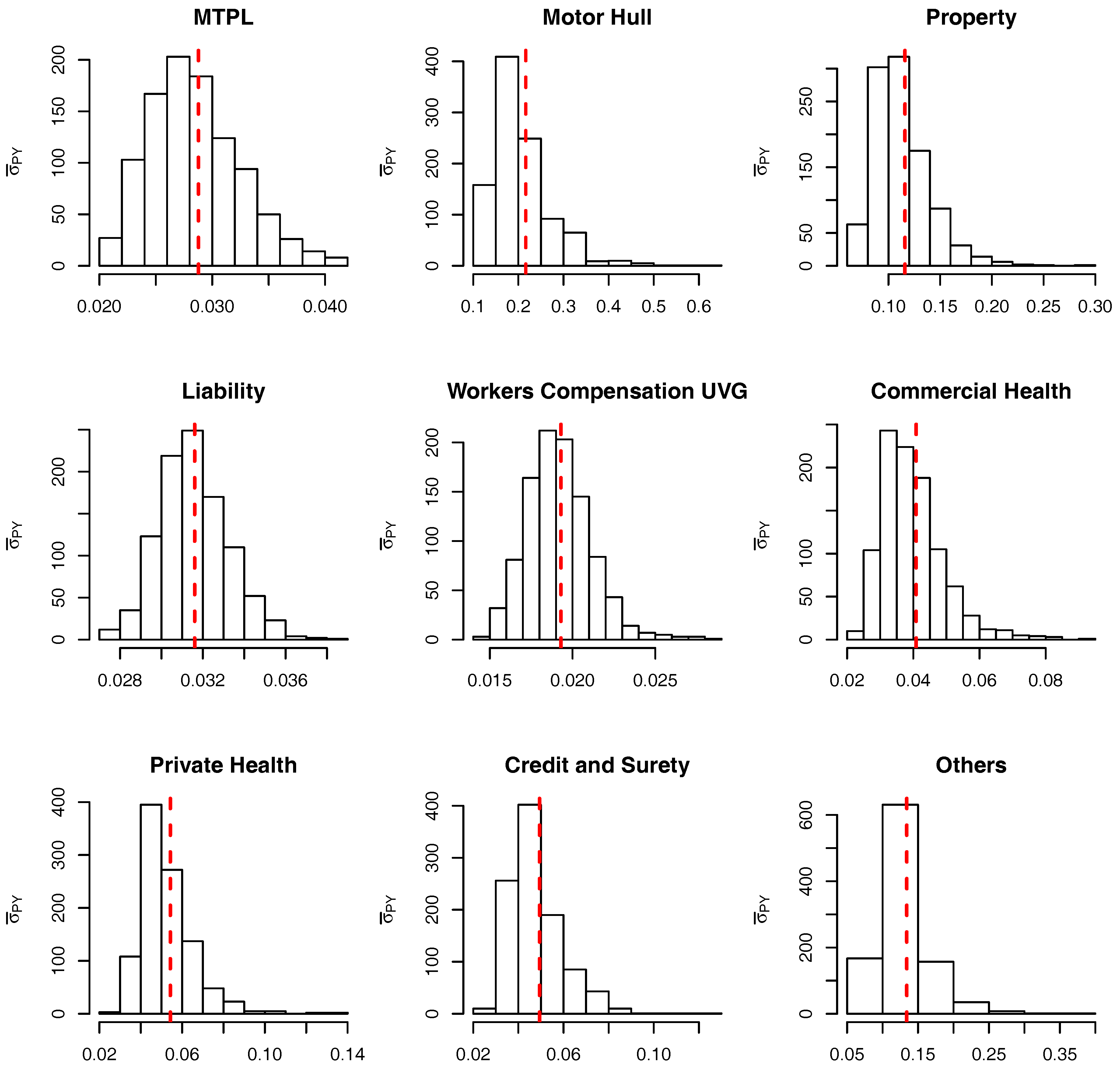
Figure 6.
Histogram of the parameter for the conditional model. Red dashed line: .

Figure 7.
Histograms levels used in the SMC sampler algorithm with in the marginalized model. The red dashed bar represents the true value of the quantile.
Figure 7.
Histograms levels used in the SMC sampler algorithm with in the marginalized model. The red dashed bar represents the true value of the quantile.

Figure 8.
Histograms levels used in the Sequential Monte Carlo (SMC) sampler algorithm with in the conditional model. The red dashed bar represents the true value of the quantile.
Figure 8.
Histograms levels used in the Sequential Monte Carlo (SMC) sampler algorithm with in the conditional model. The red dashed bar represents the true value of the quantile.
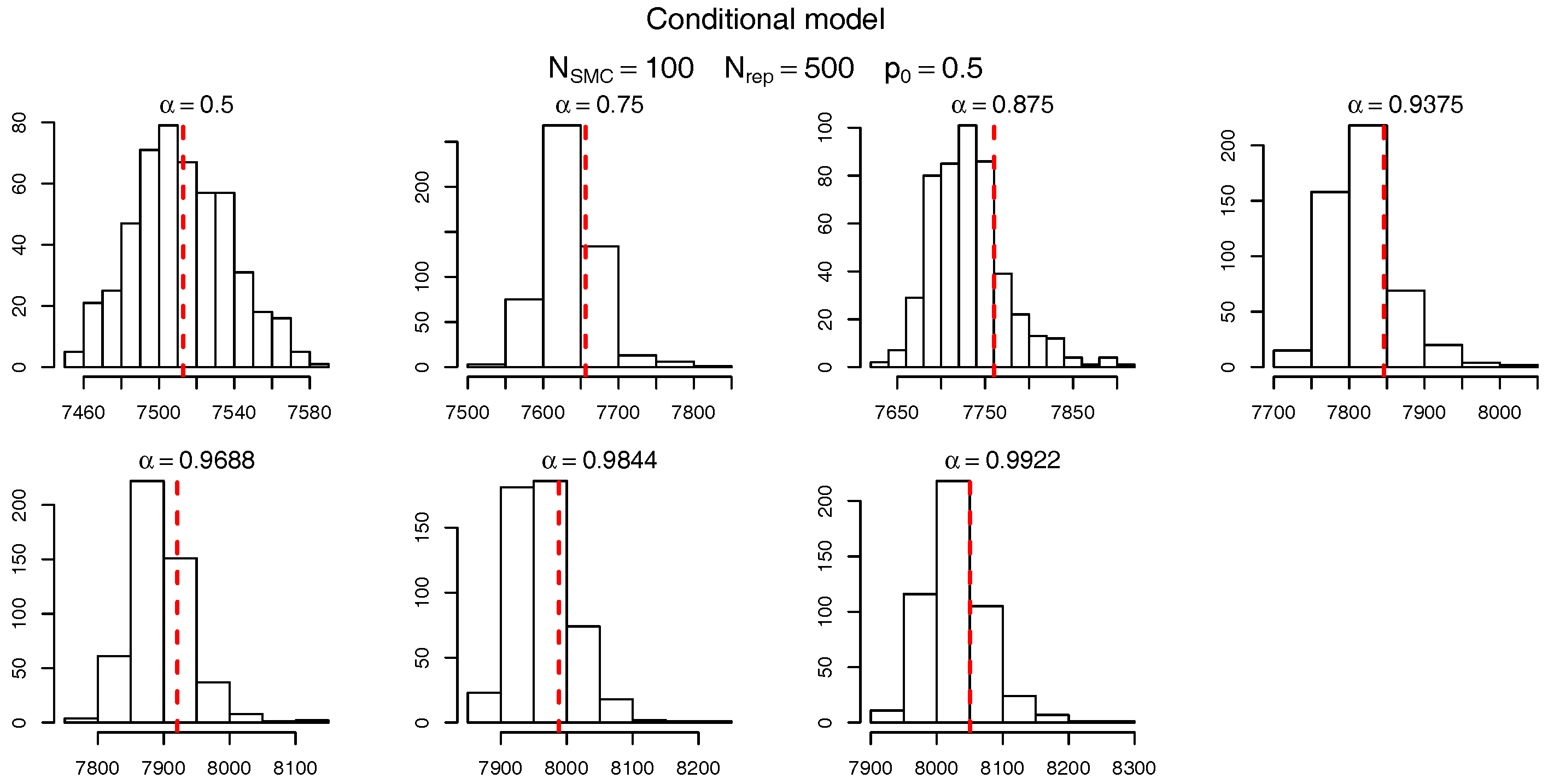
Figure 9.
Bias for the marginalized model. Note that although the bias for some of the CY large claims is around 10% their allocated capital is rather small, as seen in Figure 11 (a).
Figure 9.
Bias for the marginalized model. Note that although the bias for some of the CY large claims is around 10% their allocated capital is rather small, as seen in Figure 11 (a).

Figure 10.
Bias for the conditional model. Note that although the bias for some of the current year (CY) large claims is around 10% their allocated capital is rather small, as seen in Figure 11 (b).
Figure 10.
Bias for the conditional model. Note that although the bias for some of the current year (CY) large claims is around 10% their allocated capital is rather small, as seen in Figure 11 (b).

Figure 11.
Comparison between the “true” allocations (calculated via a large Monte Carlo procedure) and the SMC sampler solution for the (a) marginalized and (b) conditional models.
Figure 11.
Comparison between the “true” allocations (calculated via a large Monte Carlo procedure) and the SMC sampler solution for the (a) marginalized and (b) conditional models.
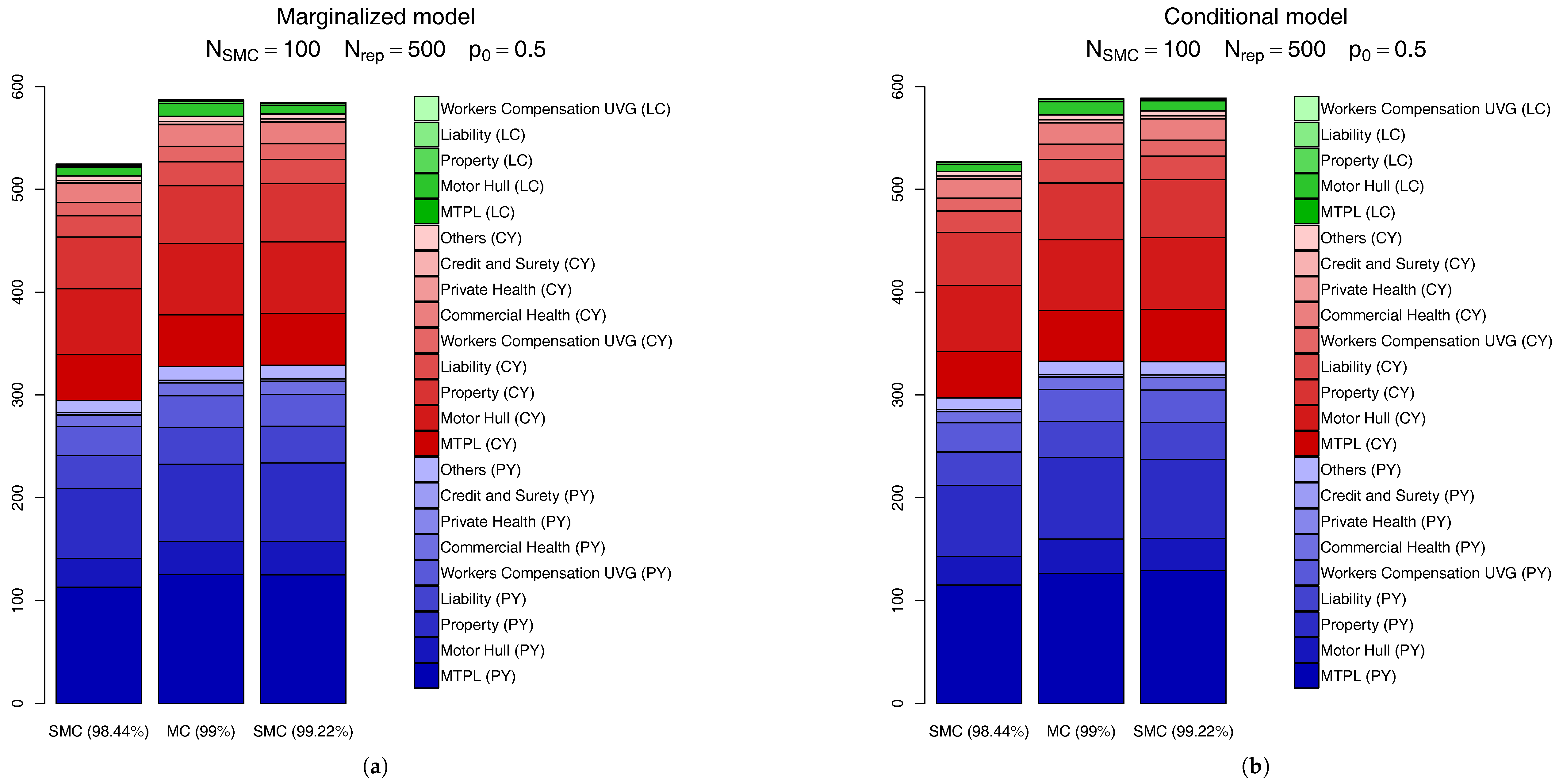
Figure 12.
Variance reduction for the marginalized model.

Figure 13.
Variance reduction for the conditional model.
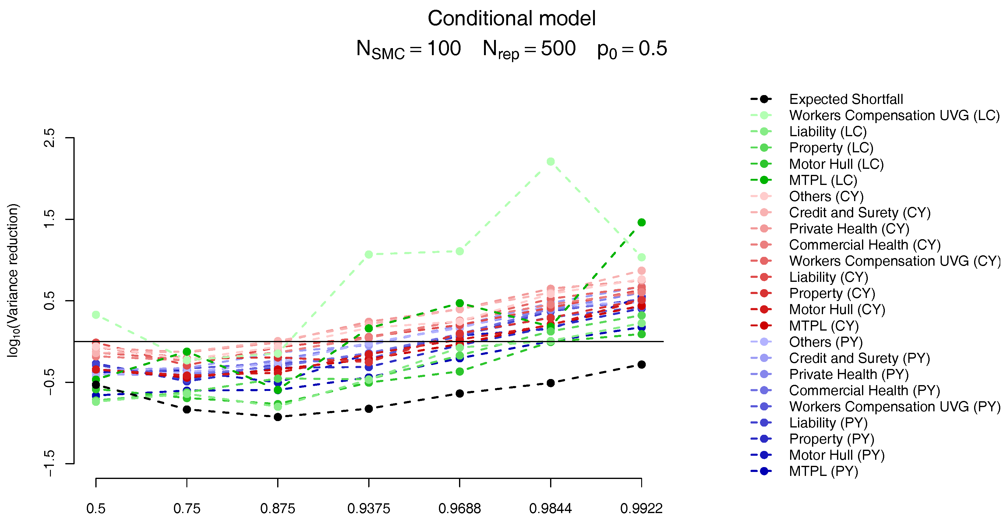
Figure 14.
Relative bias in the marginalized model as a function of (a) the parameter and (b) the sample size in the SMC sampler, .
Figure 14.
Relative bias in the marginalized model as a function of (a) the parameter and (b) the sample size in the SMC sampler, .


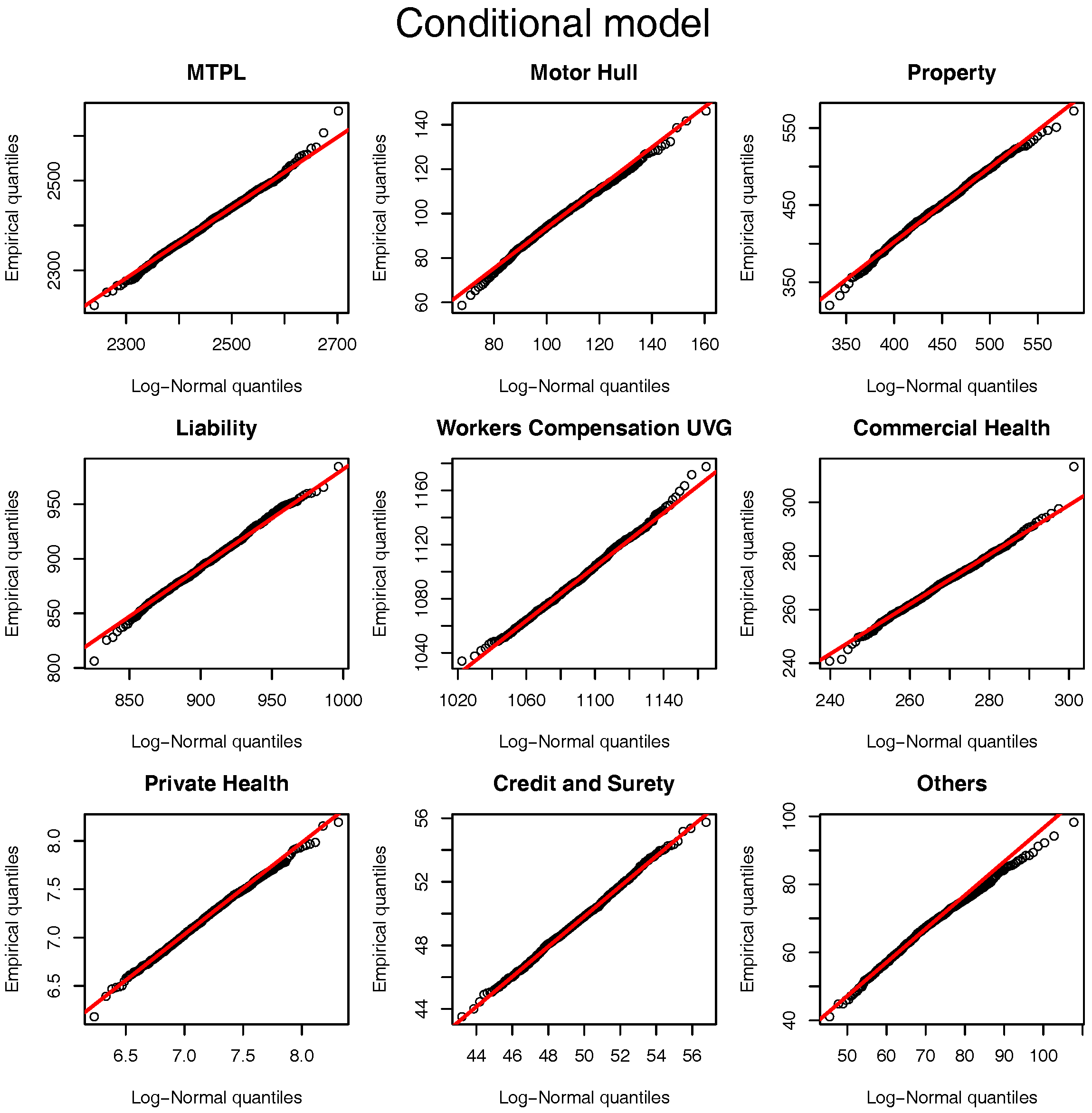
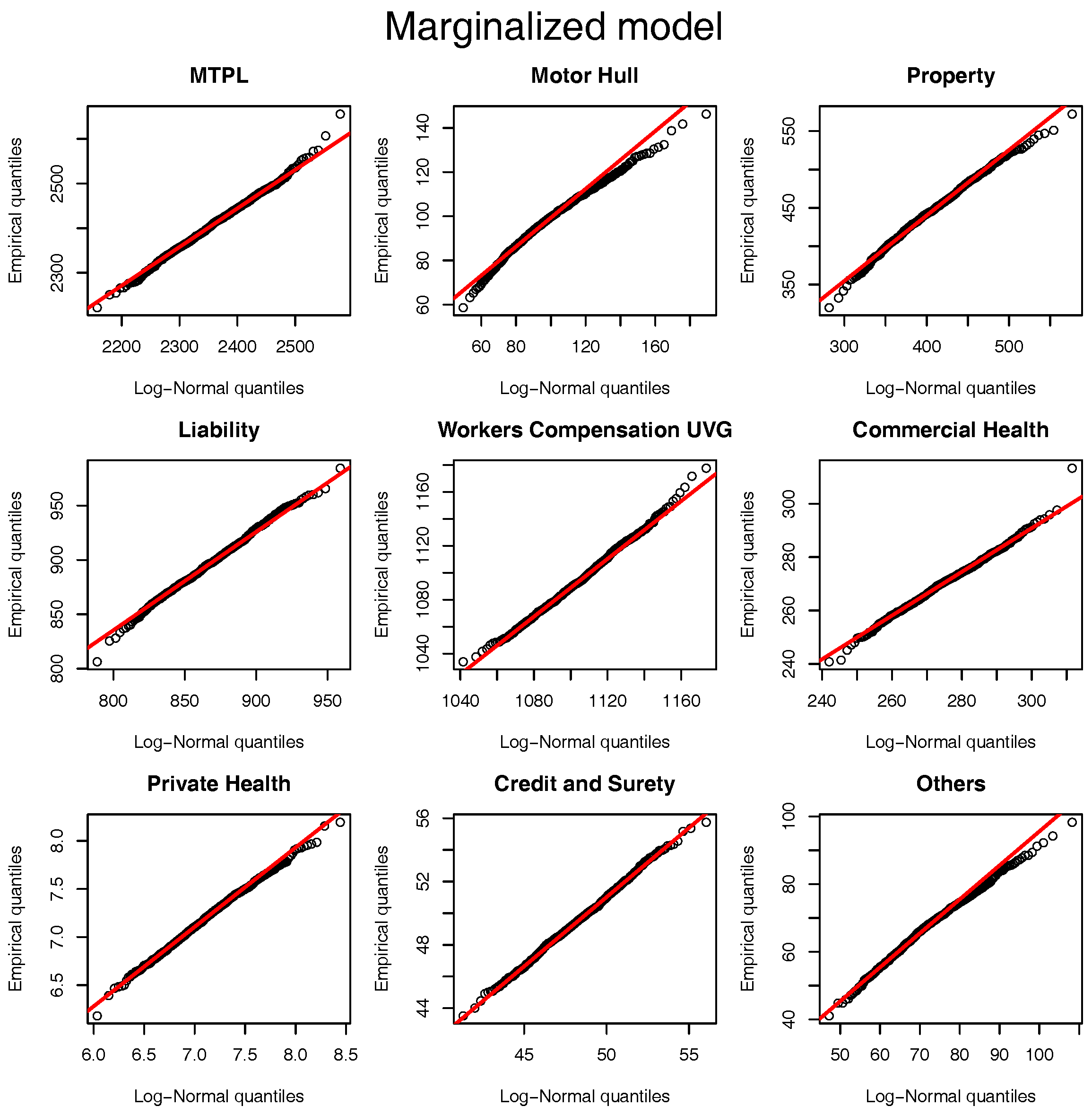
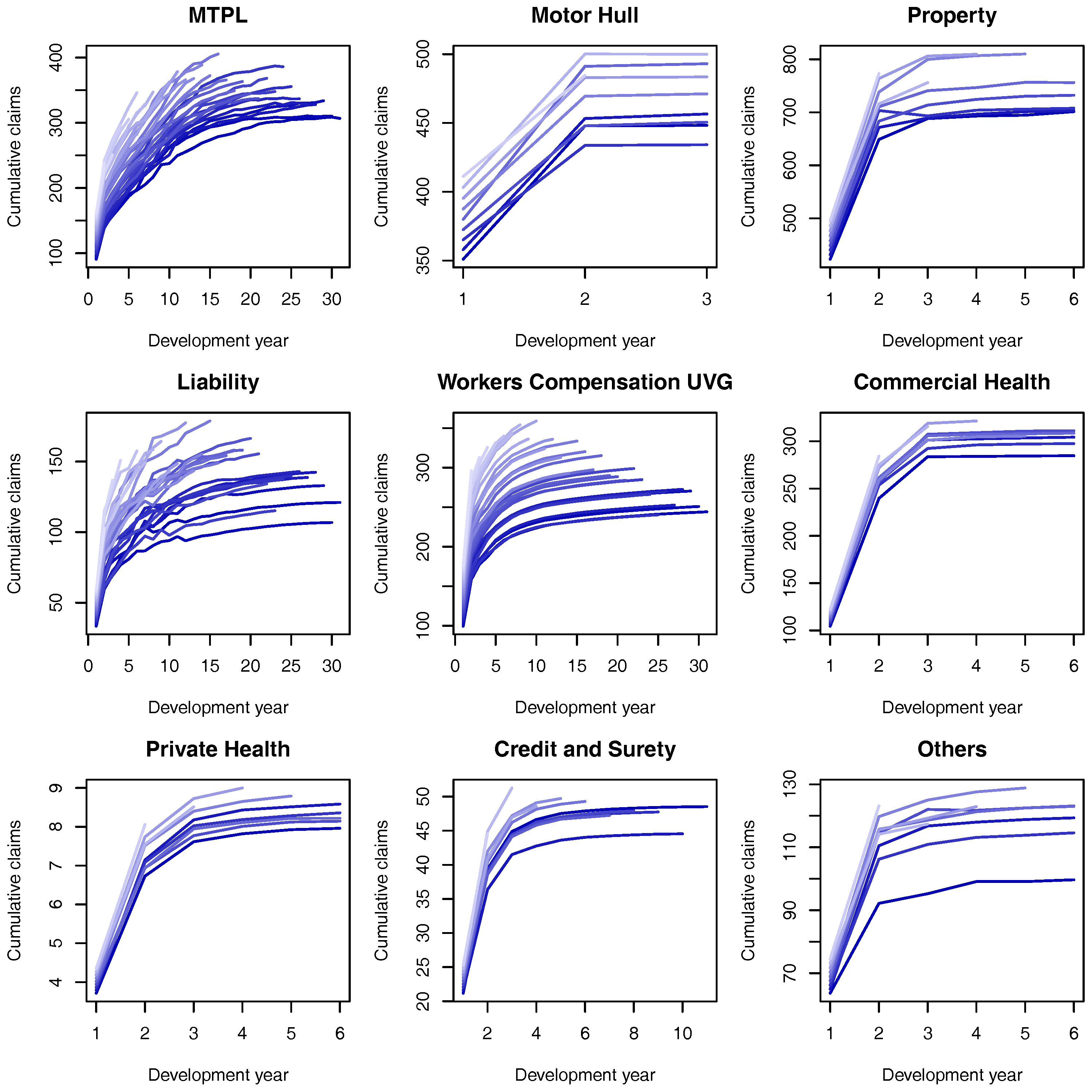
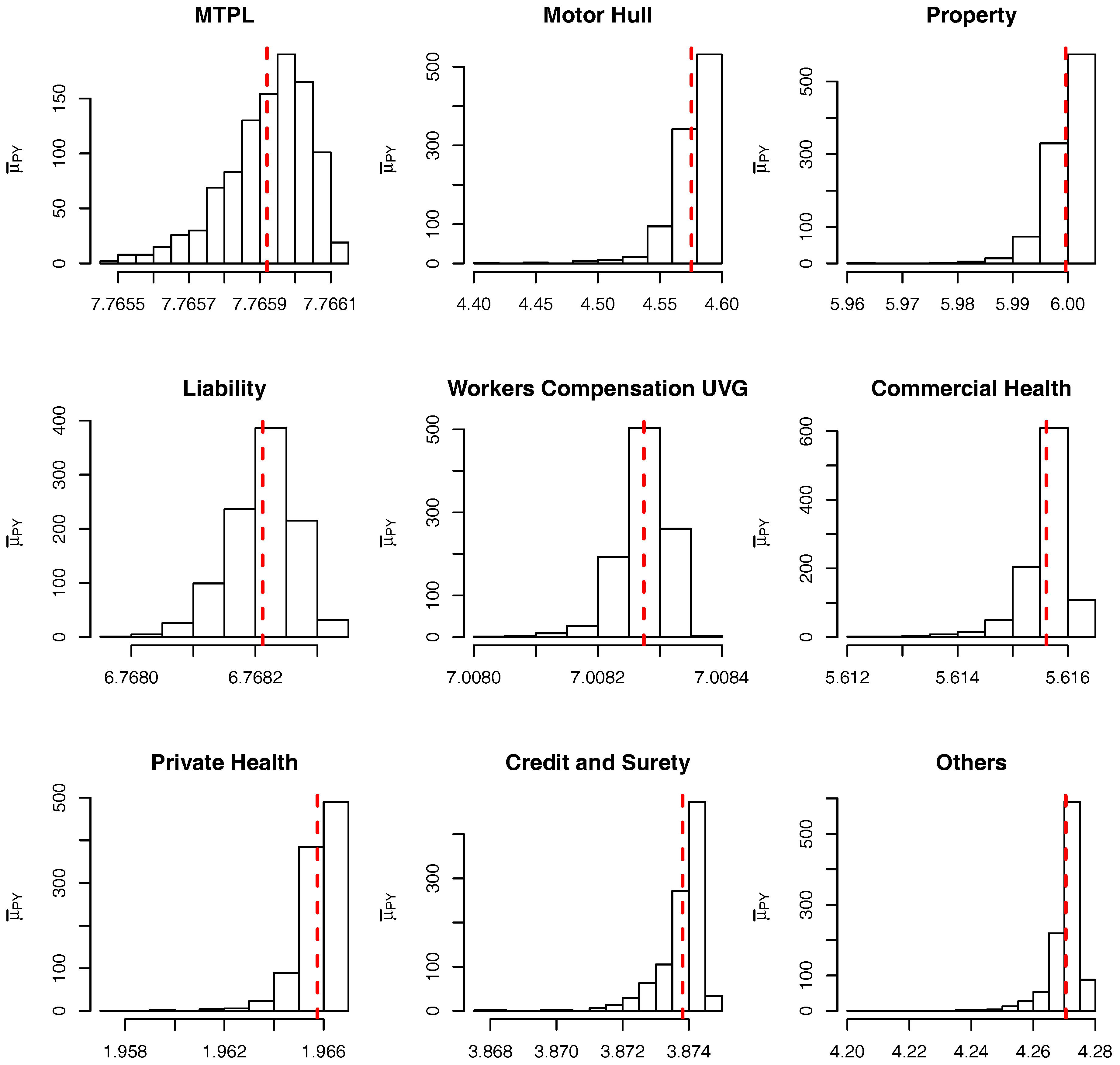
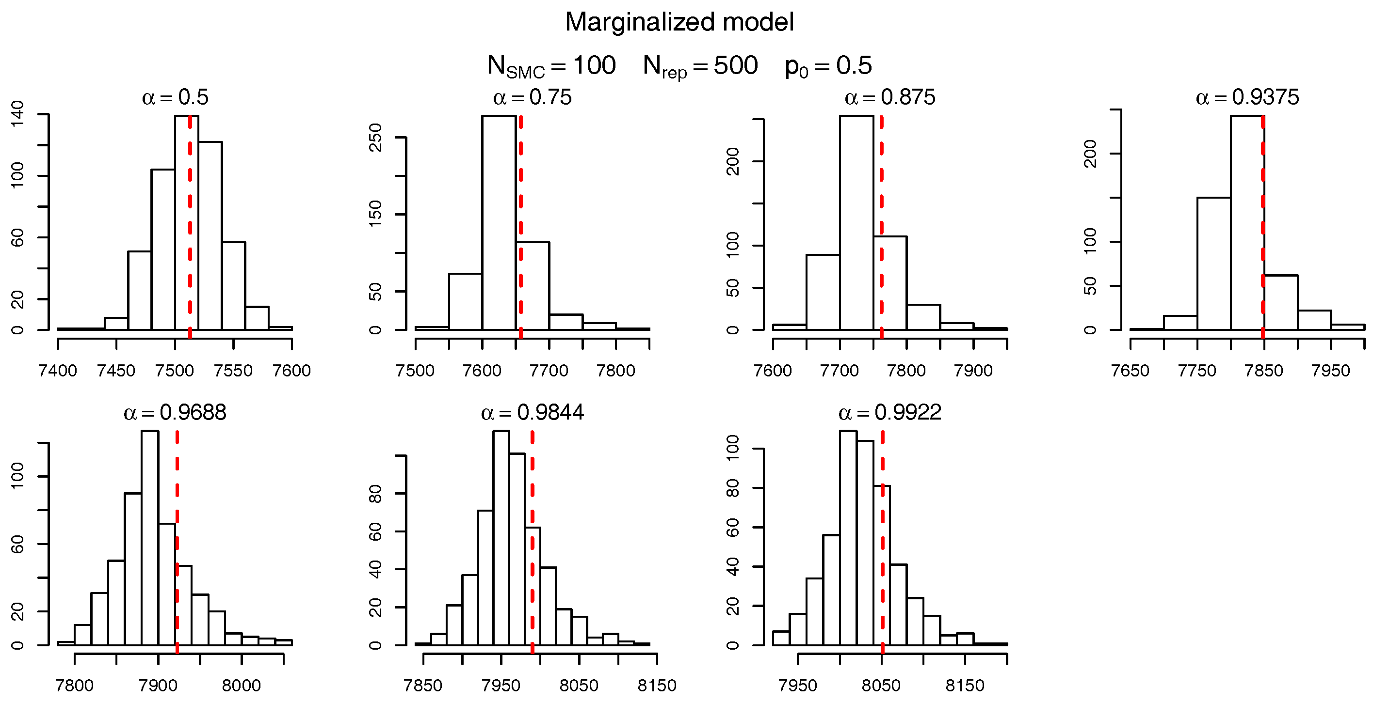
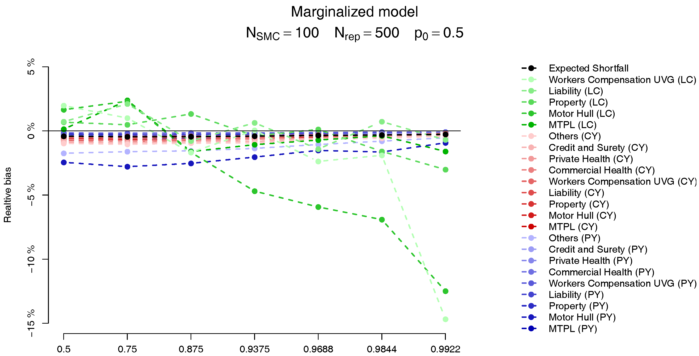
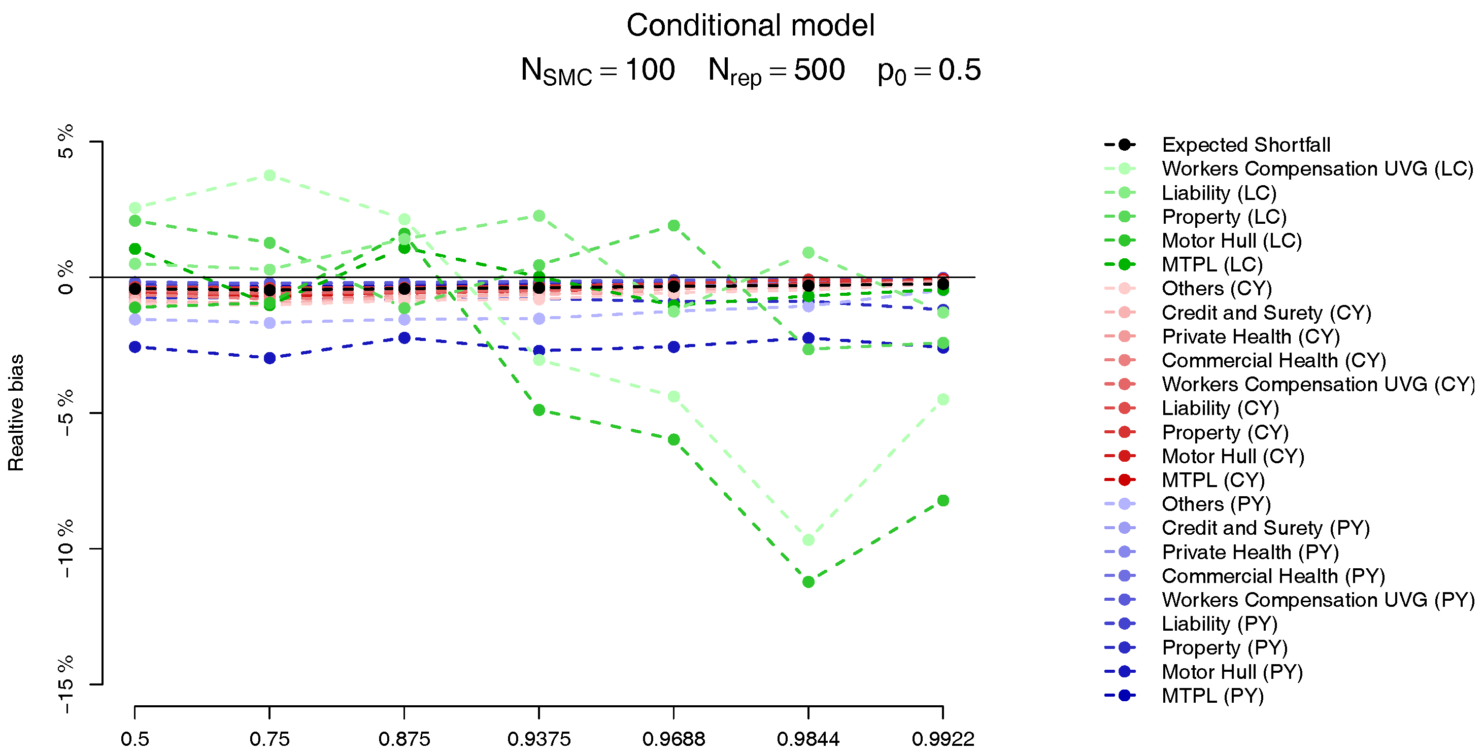
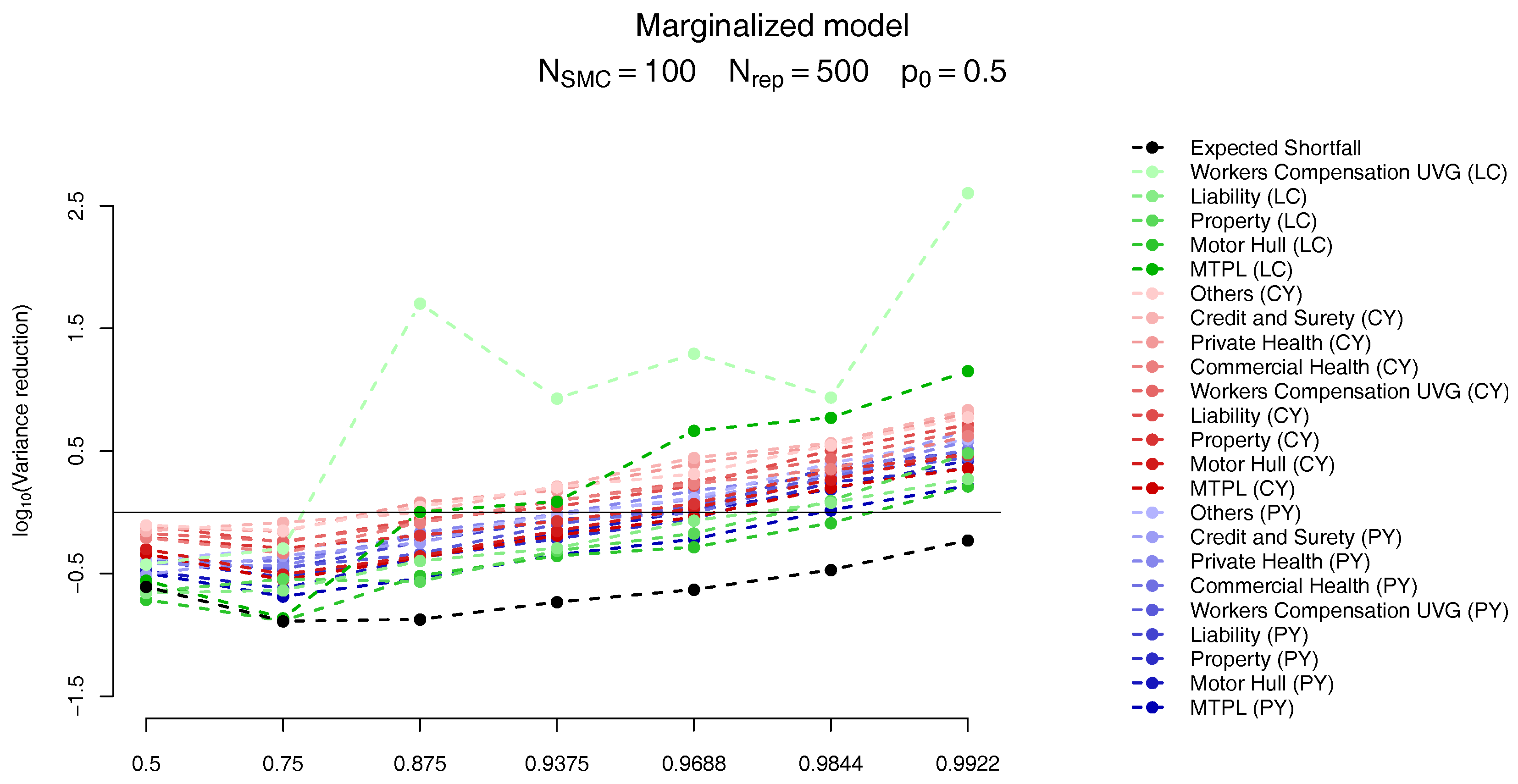
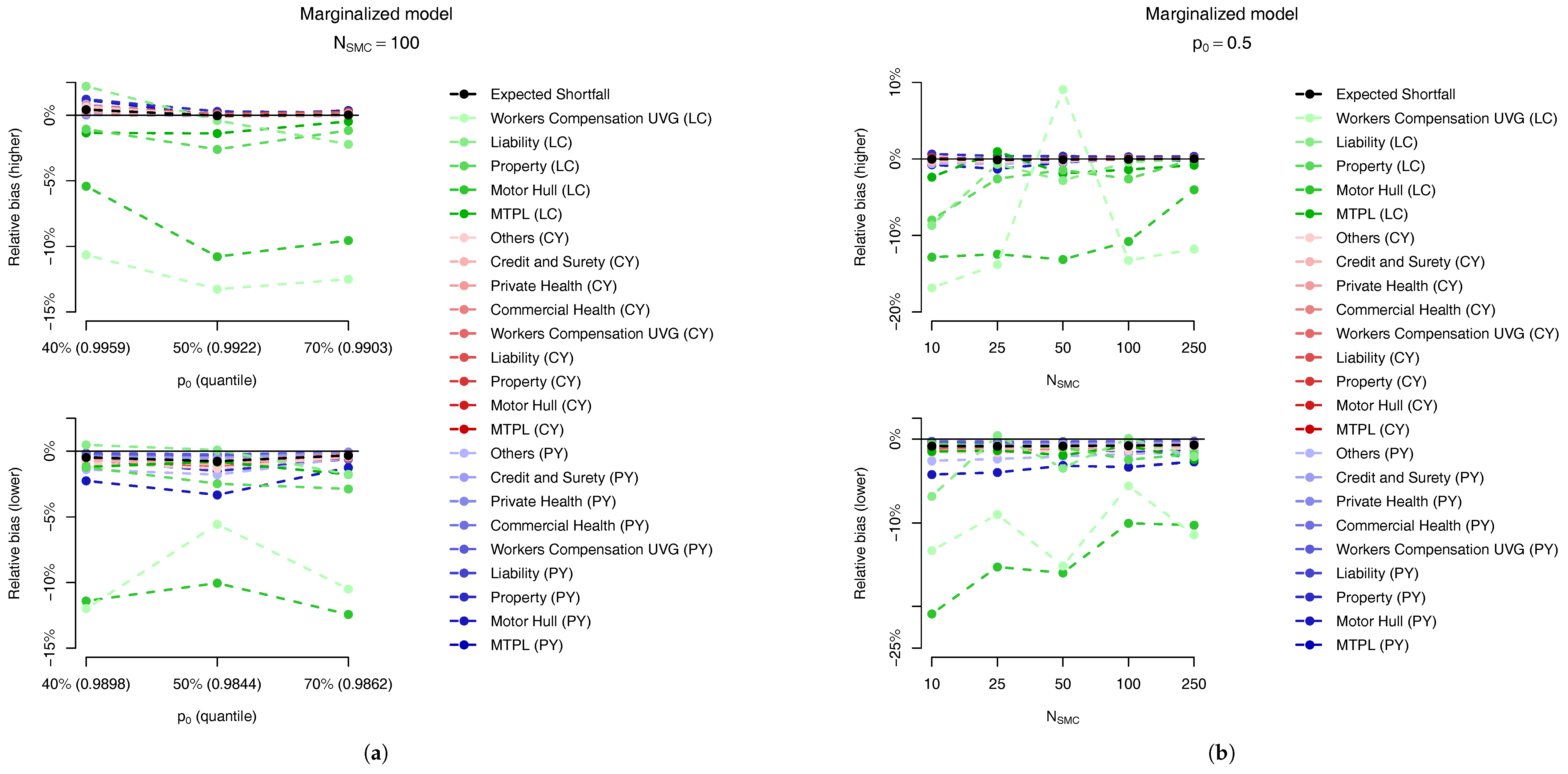
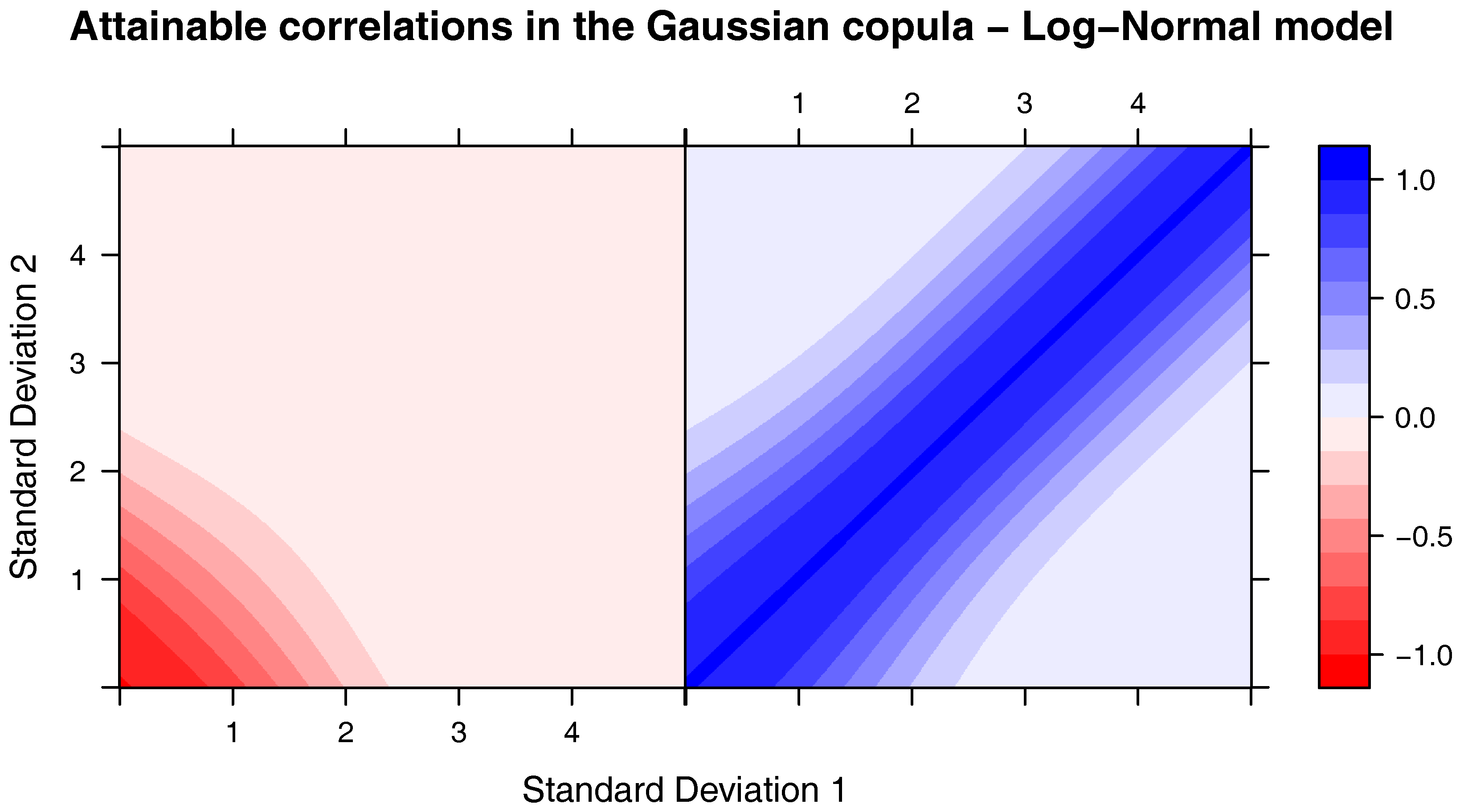
Table 1.
Initial synthetic balance sheet.
| LoB | Reserves | Premium |
|---|---|---|
| 1 MTPL | 2391.64 | 503.14 |
| 2 Motor Hull | 99.08 | 573.26 |
| 3 Property | 449.26 | 748.76 |
| 4 Liability | 870.27 | 299.73 |
| 5 Workers Compensation (UVG) | 1104.66 | 338.63 |
| 6 Commercial Health | 271.54 | 254.21 |
| 7 Private Health | 7.32 | 7.20 |
| 8 Credit and Surety | 49.50 | 34.64 |
| 9 Others | 67.64 | 46.28 |
| Total | 5310.92 | 2805.87 |
Table 2.
Parameters and capital calculations for the marginalized and conditional models.
| LoB | Reserve/ | CoVa | Expectation | Standalone | Marginalized | Conditional | |||||||
| Premium | ES | SCR | ES | SCR | Div. Benefit | ES | SCR | Div. Benefit | |||||
| 1 | 2365.44 | 0.0287 | 7.7659 | 2.87% | 2365.44 | 2546.31 | 180.87 | 2489.85 | 124.41 | 31.22% | 2492.05 | 126.61 | 30.00% |
| 2 | 99.37 | 0.2164 | 4.5755 | 21.90% | 99.37 | 173.23 | 73.86 | 131.73 | 32.36 | 56.19% | 132.59 | 33.21 | 55.03% |
| 3 | 405.99 | 0.1142 | 5.9998 | 11.46% | 405.99 | 547.25 | 141.26 | 479.11 | 73.12 | 48.24% | 485.27 | 79.28 | 43.88% |
| 4 | 870.19 | 0.0315 | 6.7682 | 3.15% | 870.19 | 946.06 | 75.87 | 905.48 | 35.29 | 53.49% | 905.29 | 35.10 | 53.73% |
| 5 | 1105.95 | 0.0193 | 7.0083 | 1.93% | 1105.95 | 1,164.04 | 58.09 | 1137.06 | 31.11 | 46.44% | 1136.88 | 30.93 | 46.76% |
| 6 | 274.91 | 0.0410 | 5.6156 | 4.10% | 274.91 | 306.43 | 31.52 | 287.33 | 12.42 | 60.59% | 286.97 | 12.06 | 61.74% |
| 7 | 7.150 | 0.0547 | 1.9657 | 5.48% | 7.15 | 8.26 | 1.11 | 7.45 | 0.30 | 73.27% | 7.43 | 0.28 | 74.50% |
| 8 | 48.18 | 0.0493 | 3.8738 | 4.93% | 48.18 | 54.89 | 6.71 | 50.51 | 2.32 | 65.36% | 50.43 | 2.25 | 66.44% |
| 9 | 72.20 | 0.1332 | 4.2706 | 13.38% | 72.2 | 102.16 | 29.96 | 85.32 | 13.12 | 56.21% | 85.15 | 12.95 | 56.77% |
| Total PY | 5249.38 | 5249.38 | 5848.63 | 599.25 | 5573.84 | 324.45 | 45.86% | 5582.06 | 332.67 | 44.49% | |||
| 1 | 503.14 | 0.0685 | 6.0958 | 6.86% | 448.94 | 533.07 | 84.13 | 499.16 | 50.21 | 40.32% | 498.37 | 49.43 | 41.25% |
| 2 | 573.26 | 0.0702 | 6.0356 | 7.03% | 402.87 | 504.20 | 101.33 | 472.25 | 69.38 | 31.53% | 471.66 | 68.79 | 32.11% |
| 3 | 748.76 | 0.0683 | 6.3013 | 6.84% | 547.23 | 654.38 | 107.15 | 603.36 | 56.13 | 47.62% | 602.61 | 55.38 | 48.31% |
| 4 | 299.73 | 0.0923 | 5.3596 | 9.25% | 216.70 | 272.05 | 55.35 | 239.69 | 22.99 | 58.47% | 239.57 | 22.87 | 58.69% |
| 5 | 338.63 | 0.0648 | 5.6841 | 6.49% | 303.77 | 349.69 | 45.92 | 319.17 | 15.40 | 66.47% | 318.71 | 14.94 | 67.45% |
| 6 | 254.21 | 0.0804 | 5.4296 | 8.05% | 228.79 | 282.62 | 53.83 | 249.63 | 20.85 | 61.28% | 249.31 | 20.52 | 61.88% |
| 7 | 7.20 | 0.1047 | 1.8628 | 10.5% | 6.48 | 8.52 | 2.04 | 7.01 | 0.53 | 73.84% | 7.01 | 0.53 | 74.06% |
| 8 | 34.64 | 0.0981 | 3.3172 | 9.84% | 27.72 | 35.84 | 8.13 | 30.32 | 2.60 | 67.95% | 30.28 | 2.57 | 68.44% |
| 9 | 46.28 | 0.1004 | 3.6066 | 10.06% | 37.03 | 48.16 | 11.14 | 41.83 | 4.81 | 56.83% | 41.79 | 4.77 | 57.19% |
| Total CY,s | 2805.85 | 2219.53 | 2688.53 | 469.02 | 2462.42 | 242.9 | 48.21% | 2459.31 | 239.8 | 48.87% | |||
| Peril | CoVa | Expectation | Standalone | Marginalized | Conditional | ||||||||
| ES | SCR | ES | SCR | Div. benefit | ES | SCR | Div. benefit | ||||||
| 1 | 2.50 | 2.80 | 3.89 | 20.14 | 16.25 | 4.03 | 0.15 | 99.1% | 4.01 | 0.12 | 99.27% | ||
| 2 | 13.35 | 300 | 1.85 | 27.08 | 191.21 | 164.13 | 39.96 | 12.88 | 92.15% | 39.61 | 12.53 | 92.36% | |
| 3 | 6.28 | 100 | 1.50 | 14.34 | 84.31 | 69.97 | 16.5 | 2.16 | 96.91% | 16.45 | 2.11 | 96.98% | |
| 4 | 3.88 | 100 | 1.80 | 8.10 | 61.34 | 53.24 | 8.94 | 0.84 | 98.42% | 8.91 | 0.81 | 98.48% | |
| 5 | 0.50 | 2.00 | 1.00 | 10.00 | 9.00 | 1.07 | 0.07 | 99.19% | 1.12 | 0.12 | 98.69% | ||
| Total CY,l | 54.41 | 367 | 312.59 | 70.5 | 16.1 | 94.85% | 70.1 | 15.69 | 94.98% | ||||
| Total | 8055.26 | 7523.32 | 8904.18 | 1380.86 | 8106.77 | 583.45 | 57.75% | 8111.5 | 588.18 | 57.40% | |||
Table 3.
Swiss Solvency Test (SST)’s (2015) standard development patterns for claims provision (normalized to have at most 30 development years and rounded to 2 digits).
Table 3.
Swiss Solvency Test (SST)’s (2015) standard development patterns for claims provision (normalized to have at most 30 development years and rounded to 2 digits).
| LoB | Year 0 | Year 1 | Year 2 | Year 3 | Year 4 | Year 5 | Year 6 | Year 7 | Year 8 | Year 9 | Year 10 | Year 11 | Year 12 | Year 13 | Year 14 | Year 15 |
| 1 | 30.18% | 15.63% | 5.78% | 4.94% | 4.43% | 4.34% | 4.09% | 3.92% | 3.66% | 3.50% | 3.08% | 2.64% | 2.16% | 1.86% | 1.50% | 1.30% |
| 2 | 81.08% | 18.67% | 0.24% | 0% | 0% | 0% | 0% | 0% | 0% | 0% | 0% | 0% | 0% | 0% | 0% | 0% |
| 3 | 58.24% | 35.06% | 4.36% | 1.37% | 0.64% | 0.33% | 0% | 0% | 0% | 0% | 0% | 0% | 0% | 0% | 0% | 0% |
| 4 | 26.55% | 23.53% | 8.33% | 6.18% | 4.79% | 4.15% | 3.63% | 3.14% | 2.55% | 2.11% | 1.80% | 1.59% | 1.35% | 1.20% | 1.12% | 1.02% |
| 5 | 40.62% | 24.92% | 7.14% | 4.86% | 4.43% | 3.13% | 2.57% | 1.67% | 1.31% | 1.22% | 1.05% | 0.69% | 0.60% | 0.56% | 0.51% | 0.47% |
| 6 | 36.83% | 47.68% | 14.20% | 0.88% | 0.28% | 0.14% | 0% | 0% | 0% | 0% | 0% | 0% | 0% | 0% | 0% | 0% |
| 7 | 46.26% | 38.05% | 10.78% | 2.94% | 1.27% | 0.69% | 0% | 0% | 0% | 0% | 0% | 0% | 0% | 0% | 0% | 0% |
| 8 | 45.85% | 35.28% | 11.35% | 3.72% | 1.62% | 0.91% | 0.52% | 0.32% | 0.20% | 0.13% | 0.10% | 0% | 0% | 0% | 0% | 0% |
| 9 | 58.24% | 35.06% | 4.36% | 1.37% | 0.64% | 0.33% | 0% | 0% | 0% | 0% | 0% | 0% | 0% | 0% | 0% | 0% |
| LoB | Year 16 | Year 17 | Year 18 | Year 19 | Year 20 | Year 21 | Year 22 | Year 23 | Year 24 | Year 25 | Year 26 | Year 27 | Year 28 | Year 29 | Year 30 | |
| 1 | 1.06% | 0.88% | 0.73% | 0.64% | 0.60% | 0.53% | 0.47% | 0.44% | 0.41% | 0.37% | 0.29% | 0.21% | 0.15% | 0.12% | 0.10% | |
| 2 | 0% | 0% | 0% | 0% | 0% | 0% | 0% | 0% | 0% | 0% | 0% | 0% | 0% | 0% | 0% | |
| 3 | 0% | 0% | 0% | 0% | 0% | 0% | 0% | 0% | 0% | 0% | 0% | 0% | 0% | 0% | 0% | |
| 4 | 0.88% | 0.77% | 0.72% | 0.66% | 0.60% | 0.55% | 0.52% | 0.49% | 0.45% | 0.4% | 0.31% | 0.22% | 0.16% | 0.13% | 0.11% | |
| 5 | 0.43% | 0.40% | 0.37% | 0.35% | 0.33% | 0.31% | 0.29% | 0.27% | 0.26% | 0.24% | 0.23% | 0.22% | 0.20% | 0.19% | 0.18% | |
| 6 | 0% | 0% | 0% | 0% | 0% | 0% | 0% | 0% | 0% | 0% | 0% | 0% | 0% | 0% | 0% | |
| 7 | 0% | 0% | 0% | 0% | 0% | 0% | 0% | 0% | 0% | 0% | 0% | 0% | 0% | 0% | 0% | |
| 8 | 0% | 0% | 0% | 0% | 0% | 0% | 0% | 0% | 0% | 0% | 0% | 0% | 0% | 0% | 0% | |
| 9 | 0% | 0% | 0% | 0% | 0% | 0% | 0% | 0% | 0% | 0% | 0% | 0% | 0% | 0% | 0% |
Table 4.
Mack’s standard deviation parameter estimates, , based on exogenous triangles and for the development lengths given in Table 3.
Table 4.
Mack’s standard deviation parameter estimates, , based on exogenous triangles and for the development lengths given in Table 3.
| LoB | Year 0 | Year 1 | Year 2 | Year 3 | Year 4 | Year 5 | Year 6 | Year 7 | Year 8 | Year 9 | Year 10 | Year 11 | Year 12 | Year 13 | Year 14 |
| 1 | 0.5673 | 0.2280 | 0.1922 | 0.2681 | 0.2683 | 0.3949 | 0.2652 | 0.2641 | 0.2789 | 0.3055 | 0.1458 | 0.1577 | 0.2140 | 0.1001 | 0.1016 |
| 2 | 0.6640 | 0.0659 | |||||||||||||
| 3 | 1.3614 | 0.4921 | 0.3215 | 0.0875 | 0.0666 | ||||||||||
| 4 | 0.8248 | 0.4328 | 0.4021 | 0.3644 | 0.3772 | 0.2729 | 0.5268 | 0.244 | 0.2786 | 0.1559 | 0.2660 | 0.0776 | 0.0757 | 0.1220 | 0.0418 |
| 5 | 0.9914 | 0.3317 | 0.1807 | 0.1072 | 0.0740 | 0.0444 | 0.0359 | 0.0255 | 0.0190 | 0.0106 | 0.0166 | 0.0094 | 0.0040 | 0.0105 | 0.0040 |
| 6 | 0.6069 | 0.2405 | 0.0597 | 0.0371 | 0.0172 | ||||||||||
| 7 | 0.1053 | 0.0450 | 0.0157 | 0.0113 | 0.0091 | ||||||||||
| 8 | 0.3098 | 0.0737 | 0.0310 | 0.0203 | 0.0137 | 0.0051 | 0.0020 | 0.0026 | 0.0020 | 0.0014 | 0.0011 | ||||
| 9 | 0.9163 | 0.1910 | 0.1248 | 0.0340 | 0.0258 | ||||||||||
| LoB | Year 15 | Year 16 | Year 17 | Year 18 | Year 19 | Year 20 | Year 21 | Year 22 | Year 23 | Year 24 | Year 25 | Year 26 | Year 27 | Year 28 | Year 29 |
| 1 | 0.0466 | 0.1097 | 0.1081 | 0.0583 | 0.1353 | 0.0916 | 0.0916 | 0.0916 | 0.0916 | 0.0916 | 0.0916 | 0.0916 | 0.0916 | 0.0916 | 0.0916 |
| 2 | |||||||||||||||
| 3 | |||||||||||||||
| 4 | 0.0272 | 0.0886 | 0.0422 | 0.0190 | 0.0238 | 0.0190 | 0.0152 | 0.0122 | 0.0097 | 0.0078 | 0.0062 | 0.0050 | 0.0040 | 0.0032 | 0.0025 |
| 5 | 0.0040 | 0.0040 | 0.0040 | 0.0040 | 0.0040 | 0.0040 | 0.0040 | 0.0040 | 0.0040 | 0.0040 | 0.0040 | 0.0040 | 0.0040 | 0.0040 | 0.0040 |
| 6 | |||||||||||||||
| 7 | |||||||||||||||
| 8 | |||||||||||||||
| 9 |
Table 5.
Claims ratio, average claim amount (in millions of CHF) and market share.
| LoB | Claims Ratio | Average Claim Amount | Market Share |
|---|---|---|---|
| 1 | 90% | 0.005 | |
| 2 | 75% | 0.003 | 20% |
| 3 | 75% | 0.004 | |
| 4 | 75% | 0.004 | |
| 5 | 90% | 0.004 | 10% |
| 6 | 90% | 0.003 | |
| 7 | 90% | 0.002 | |
| 8 | 80% | 0.003 | |
| 9 | 80% | 0.003 |
Table 6.
Copula correlation matrix from the marginalized model. Correlation block for the marginalized model: (Table 7); (Table 8); (Table 9).
Table 7.
Correlation block for the marginalized model: .
| LoB | 1 | 2 | 3 | 4 | 5 | 6 | 7 | 8 | 9 |
|---|---|---|---|---|---|---|---|---|---|
| 1 | 1 | 0.1517 | 0.1505 | 0.2501 | 0.5001 | 0.2501 | 0.1501 | 0.2502 | 0.2511 |
| 2 | 1 | 0.1520 | 0.1517 | 0.1517 | 0.1517 | 0.1517 | 0.1517 | 0.2532 | |
| 3 | 1 | 0.1505 | 0.1505 | 0.1505 | 0.1505 | 0.1505 | 0.2515 | ||
| 4 | 1 | 0.2501 | 0.1501 | 0.1501 | 0.1501 | 0.2511 | |||
| 5 | 1 | 0.2501 | 0.1501 | 0.2501 | 0.2511 | ||||
| 6 | 1 | 0.1501 | 0.2502 | 0.2511 | |||||
| 7 | 1 | 0.1502 | 0.2511 | ||||||
| 8 | 1 | 0.2511 | |||||||
| 9 | 1 |
Table 8.
Correlation block for the marginalized model: .
| LoB | 1 | 2 | 3 | 4 | 5 | 6 | 7 | 8 | 9 |
|---|---|---|---|---|---|---|---|---|---|
| 1 | 0.5004 | 0.5005 | 0.1502 | 0.2505 | 0.2503 | 0.2504 | 0.1504 | 0.2506 | 0.2506 |
| 2 | 0.5046 | 0.5046 | 0.2528 | 0.1519 | 0.2528 | 0.1518 | 0.1519 | 0.1519 | 0.2529 |
| 3 | 0.1506 | 0.2509 | 0.5013 | 0.2510 | 0.1506 | 0.1506 | 0.1508 | 0.1507 | 0.2511 |
| 4 | 0.2503 | 0.1502 | 0.2503 | 0.5008 | 0.1502 | 0.1503 | 0.1504 | 0.1504 | 0.2506 |
| 5 | 0.2503 | 0.2503 | 0.1502 | 0.1503 | 0.5004 | 0.2504 | 0.1504 | 0.2506 | 0.2506 |
| 6 | 0.2503 | 0.1502 | 0.1502 | 0.1503 | 0.2503 | 0.5006 | 0.2507 | 0.2506 | 0.2506 |
| 7 | 0.1502 | 0.1503 | 0.1502 | 0.1504 | 0.1502 | 0.2505 | 0.5010 | 0.1504 | 0.2506 |
| 8 | 0.2503 | 0.1502 | 0.1502 | 0.1504 | 0.2503 | 0.2504 | 0.1504 | 0.5009 | 0.2506 |
| 9 | 0.2511 | 0.2511 | 0.2511 | 0.2513 | 0.2511 | 0.2512 | 0.2514 | 0.2513 | 0.5018 |
Table 9.
Correlation block for the marginalized model: .
| LoB | 1 | 2 | 3 | 4 | 5 | 6 | 7 | 8 | 9 |
|---|---|---|---|---|---|---|---|---|---|
| 1 | 1 | 0.5006 | 0.1503 | 0.2506 | 0.2504 | 0.1504 | 0.1505 | 0.1505 | 0.2507 |
| 2 | 1 | 0.2505 | 0.1504 | 0.2504 | 0.1504 | 0.1505 | 0.1505 | 0.2507 | |
| 3 | 1 | 0.2506 | 0.1503 | 0.1504 | 0.1505 | 0.1505 | 0.2507 | ||
| 4 | 1 | 0.1504 | 0.1505 | 0.1506 | 0.1506 | 0.2509 | |||
| 5 | 1 | 0.2505 | 0.1505 | 0.2507 | 0.2507 | ||||
| 6 | 1 | 0.2508 | 0.2508 | 0.2508 | |||||
| 7 | 1 | 0.1507 | 0.2510 | ||||||
| 8 | 1 | 0.2509 | |||||||
| 9 | 1 |
Table 10.
Intermediate quantiles for different values of .
| 1 | 2 | 3 | 4 | 5 | 6 | 7 | |
| 0.4 | 0.6 | 0.84 | 0.936 | 0.9744 | 0.9898 | 0.9959 | |
| 0.5 | 0.5 | 0.75 | 0.875 | 0.9375 | 0.9688 | 0.9844 | 0.9922 |
| 0.7 | 0.3 | 0.51 | 0.657 | 0.7599 | 0.8319 | 0.8824 | 0.9176 |
| 8 | 9 | 10 | 11 | 12 | 13 | ||
| 0.4 | |||||||
| 0.5 | |||||||
| 0.7 | 0.9424 | 0.9596 | 0.9718 | 0.9802 | 0.9862 | 0.9903 |
© 2017 by the authors. Licensee MDPI, Basel, Switzerland. This article is an open access article distributed under the terms and conditions of the Creative Commons Attribution (CC BY) license (http://creativecommons.org/licenses/by/4.0/).
Share and Cite
MDPI and ACS Style
Peters, G.W.; Targino, R.S.; Wüthrich, M.V. Bayesian Modelling, Monte Carlo Sampling and Capital Allocation of Insurance Risks. Risks 2017, 5, 53. https://doi.org/10.3390/risks5040053
AMA Style
Peters GW, Targino RS, Wüthrich MV. Bayesian Modelling, Monte Carlo Sampling and Capital Allocation of Insurance Risks. Risks. 2017; 5(4):53. https://doi.org/10.3390/risks5040053
Chicago/Turabian StylePeters, Gareth W., Rodrigo S. Targino, and Mario V. Wüthrich. 2017. "Bayesian Modelling, Monte Carlo Sampling and Capital Allocation of Insurance Risks" Risks 5, no. 4: 53. https://doi.org/10.3390/risks5040053
Note that from the first issue of 2016, this journal uses article numbers instead of page numbers. See further details here.