
Deflation Risk and Implications for Life Insurers

Department of Statistics and Actuarial Science, Simon Fraser University, 8888 University Drive, Burnaby, BC V5A 1S6, Canada
Risks 2016, 4(4), 46; https://doi.org/10.3390/risks4040046
Submission received: 26 August 2016
/
Revised: 25 November 2016
/
Accepted: 28 November 2016
/
Published: 3 December 2016
Abstract
:Life insurers are exposed to deflation risk: falling prices could lead to insufficient investment returns, and inflation-indexed protections could make insurers vulnerable to deflation. In this spirit, this paper proposes a market-based methodology for measuring deflation risk based on a discrete framework: the latter accounts for the real interest rate, the inflation index level, its conditional variance, and the expected inflation rate. US inflation data are then used to estimate the model and show the importance of deflation risk. Specifically, the distribution of a fictitious life insurer’s future payments is investigated. We find that the proposed inflation model yields higher risk measures than the ones obtained using competing models, stressing the need for dynamic and market-consistent inflation modelling in the life insurance industry.
Keywords:
deflation risk; life insurance; risk management; unscented Kalman filter; inflation caps and floorsJEL:
C32; E31; G221. Introduction
Fluctuation in the general price level of goods and services is reflected through the inflation rate. Despite rather small changes in the inflation rate over the past two decades, the last recession created the potential for price instability.
Before the Great Recession, inflation risk was typically associated with high inflation rates. Events such as the Great Inflation of the 1970s are notable for steep inflation rates and could explain, to some extent, the common misconception that links inflation risk to high inflation rates. Yet, lately, inflation risk has become much more symmetric, and a fear that inflation may fall too low has emerged (so-called deflation). For instance, some recent actions undertaken by the Federal Reserve (Fed) in the US have been motivated by this fear of deflation, and an important number of European countries have had deflation issues in the past few years. Deflation is one of the most challenging risks faced by central banks nowadays.
In the long-run, insurance contracts, reserves, investment policies, and pension liabilities are sensitive to unexpected inflation.1 Long-term liabilities could be much worse if the inflation rate suddenly changes (e.g., see Bohnert et al. [1]). In addition, asset returns are tied up to the inflation, meaning that portfolio income could be quite dependent on the prevailing inflation rate.
Life insurers have an uncommonly large vulnerability to deflation risk: falling prices could lead to insufficient investment returns to support the rate credited to policyholders. Deflation is indeed “the worst possible world for a life insurance company” (see Mittelstaedt [2]). Japan is a notable example of how deflation can impact the life insurance business. The historical Japanese inflation rate remained below zero for most of the last twenty years, and this episode of deflation provoked the bankruptcy of at least eight Japanese insurers since 1996.
Life insurers are also vulnerable to embedded optionalities in the design of their products. For instance, inflation-indexed annuities often provide additional protection that increases the paid amount in the case of positive inflation, but does not reduce the amount in the case of deflation. This added protection is similar to an inflation floor, as the annuitant is covered against decreases in the general price level of goods and services.
On a similar note, inflation-indexed defined-benefit pension plans also provide the same kind of protection to their participants: in many instances, a decrease of the Consumer Price Index (CPI) would not reduce the retirement benefit amount.2 As an increasing number of plan sponsors decide to de-risk their financial exposures by buying special annuities, they transfer their interest rate, longevity, and deflation risks to life insurance companies. These life insurers issue pension buy-in and buy-out annuities, similar to portfolios of inflation-indexed annuities, thus exposing themselves to additional deflation risk.
Oddly, inflation is only indirectly measured by insurance companies in general [3], and Solvency II does not directly account for inflation risk. As deflation risk could have a significant impact on life insurers’ portfolios, it should be incorporated into the insurers’ enterprise risk management (ERM) framework consistently. Market-consistency is important, as an ERM framework must be able to capture the changing economic conditions. Further, new solvency regulations force insurance companies to assess their liabilities using “mark-to-market” approaches. As a matter of fact, market-consistency requires the use of models with sufficient degrees of freedom to integrate all relevant market data [4]. In this spirit, this paper presents a market-based methodology for measuring deflation risk based on a discrete framework inspired by Fisher’s [5] equation. The model accounts for the real interest rate, the inflation index level, its conditional variance, and the expected inflation rate. The real interest rate and the expected inflation rate both follow a first-order autoregressive (AR) model. The conditional variance follows the generalized autoregressive conditional heteroskedasticity (GARCH) model of Heston and Nandi [6]. This approach is somewhat different from common practice, as we model both the real interest rate and the expected inflation separately.3 The dynamics used in this paper are in line with the inflation modelling literature. Fleckenstein et al. [7] use a similar model to assess deflation risk, although their continuous-time model does not allow for heteroskedasticity in the index price level. A regime-switching first-order AR model for the expected inflation rate is proposed by Ahlgrim and D’Arcy [8]. The authors’ model is a generalization of Wilkie’s [9] inflation model, as it allows for different parameters, depending on the prevailing regime. Singor et al. [10] consider a Heston [11] type framework to model the inflation index, thus considering a dynamic variance process as is the case in this study. Ang et al. [12] consider, among other things, autoregressive moving-average (ARMA) models and Phillips [13] curve to model the inflation rate.4
As is commonly the case with tail risks, deflation is hard to quantify using classic econometric methods. For instance, Ang et al. [12] use a large number of models based on time series of inflation to assess inflation forecasting, and conclude that these models perform weakly in forecasting the first moment of inflation. In addition, even though they conclude that survey data perform better, these provide little or no evidence of potential deflation risk.
In the light of this issue, assessing deflation risk would require more than just past inflation rate data. Fortunately, a considerable amount of inflation-dependent securities are available, and their prices shall inform us on the likelihood of deflation over a given time horizon. Inflation-indexed bonds are securities that protect the investors’ purchasing-power by adjusting the principal based on changes in an inflation index. Most of the developed countries issue these bonds, yet US Treasury Inflation-Protected Securities (TIPS) are the most liquid ones, with about $500 billion in issuance. Inflation swaps are also available for most developed countries. In the US, they were introduced at the same time as TIPS, in 1997. The notional size of the US inflation swap market is estimated to be hundreds of billions [14]. A parallel market for inflation option exists; it started in 2002 with the introduction of caps and floors on the realized inflation rate. According to Fleckenstein et al. [7], the inflation option market is sufficiently liquid: active quotations are available since 2009 for a broad range of maturities and strikes.
To estimate our model, multiple types of data source are used, since inflation index levels would only capture the average expected inflation rate and not the tails of the index level distribution. Characterizing the entire index level distribution is of paramount importance in this study, because deflation risk is related to the left tail of this distribution. Thus, in addition to inflation index levels, we include nominal risk-free bonds, inflation swaps, and inflation options to the model estimation, as these securities contain relevant information about the tails of the distribution. The four types of data used in this paper are similar to what other inflation studies have utilized. For instance, Ang et al. [12] and Ahlgrim and D’Arcy [8] use time series of realized inflation rates, which is technically the same as using the index level.5 Inflation option market prices were used by Singor et al. [10], and Kitsul and Wright [15]. Fleckenstein et al. [7] employed swap prices and option data, as in this study.
An estimation method based on the unscented Kalman filter (UKF) is considered. All physical and risk-neutral parameters are estimated using likelihood maximization in a unique stage. The proposed method contrasts with other methods used in the literature (i.e., calibration techniques and multi-stage estimations). On one hand, calibration methods such as the one used by Singor et al. [10] select the model parameters based on a given day’s available prices. Even though this methodology can give a set of parameters that is consistent with market prices, it is impossible to know whether these are robust in time. In addition, only risk-neutral parameters can be inferred, since physical parameters are not directly involved in the pricing of derivatives. On the other hand, multi-stage methods, such as the one presented by Fleckenstein et al. [7], can be inadequate to capture the interaction among various model parameters, and also lack formal proofs of their effectiveness.
Another interesting consequence of using the UKF-based approach is that the expected inflation rate is forward-looking, as it is based on the current market prices. The model adapts readily to new market conditions, and the expected inflation rate is then consistent with investors’ expectations.
To estimate the model, US inflation data are used. The unconditional annualized long-term trend of expected inflation is about 1.8%, which is consistent with the Fed desired target range for inflation—between 1.7% and 2.0%. The evolution of the expected inflation is dependent on the current economic conditions: for instance, during the pre-recession era, the average expected inflation was about 3.4%, whereas its average is about 0.8% in the post-recession period. Deflation risk changes over time, with average 1-year deflation probabilities of 4%, 18%, and 29% for the pre-recession, recession, and post-recession eras, respectively.
The effects of deflation risk are assessed in the life insurance industry. In this spirit, the distribution of a fictitious life insurer’s future payments in present value is investigated. On average, the proposed inflation model yields risk measures that are higher than the ones obtained with competing models. The right tail of the future payments distribution is fatter, as low inflation scenarios are taken into consideration, and this is according to the current market conditions. The importance of modelling adequately embedded optionalities is also shown; an inflation-indexed annuity for which the paid amounts do not decrease when the inflation index level declines is used. The results show that deflation could have a notable impact on life insurers when inflation protections are embedded in the product design.
The contributions of this paper are manifold. First, a modelling framework is constructed to capture the desired empirical facts, such as correlation between the real interest rate and the expected inflation, as well as conditional heteroskedasticity. This model allows for derivative prices in closed or semi-closed form solutions. Second, forward-looking and market-consistent assessment regarding deflation can be done using the framework. Option data are useful in capturing the tails of the expected inflation distribution, and the filter-based methodology allows for dynamic risk assessments that are consistent with market participants’ expectations. This is of utmost importance, as new solvency regulations require insurers to assess their risk in a market-consistent way. Finally, our last contribution is to apply various models—full and nested frameworks—to assess, in the context of a life insurer, the importance of the two core components of the nominal interest rate: the real interest rate and the expected inflation. Based on two different exercises, we show that the full framework allows for more flexibility and a better understanding of deflation risk.
The remainder of the paper is organized as follows. Section 2 introduces the inflation framework. The estimation procedure is explained in Section 3. In Section 4, the estimation procedure is applied to US inflation data. Section 5 shows examples of how deflation risk can affect the life insurance industry. Finally, Section 6 concludes.
2. Framework
A discrete-time model for both inflation and real interest rate dynamics is presented in this section. Physical and risk-neutral dynamics are derived. The latter are of utmost importance for valuing derivatives such as bonds, inflation swaps, and inflation options.
2.1. Inflation and Real Interest Rate Dynamics
The Fisher [5] equation links nominal and real interest rates. Basically, the difference between the two interest rates is given by the expected inflation. Let be the nominal risk-free interest rate, defined as:
where is the real risk-free interest rate at time t, and is the expected inflation at time t.
Under the physical measure , the real interest rate dynamics are given by an autoregressive model:
where is a sequence of standardized Gaussian random variables. This model is equivalent to a discretized version of Vasicek [16]. Parameters θ and κ represent the unconditional level of real interest rate and the speed of mean reversion, respectively. The volatility of the real interest rate innovations is given by parameter σ.
There are many possible model formulations for modelling inflation, as explained in the introduction of this study.6 Even though the inflation index does not require an elaborate model per se, trying to fit various sources of information under a simple framework would be futile, as it cannot reflect the complexity of the inflation’s distribution and its evolution in time. Therefore, a flexible model is proposed. The latter allows for heteroskedastic innovations in the inflation index level, as well as stochastic expected inflation rate. Since time series and prices are observed on a discrete basis, the proposed framework is a discrete-time model. This would also come in handy in the estimation procedure explained in the subsequent section.
Let denote the inflation index level at time t. Under the physical measure , the log-inflation index level dynamics are given by
where is the conditional variance at time t. Moreover, and are two sequences of standardized Gaussian random variables. The real interest rate noises are correlated with the ones of the expected inflation rate; i.e., . The other sequences are uncorrelated.
Equation (3) includes a convexity correction term (i.e., ). Indeed, this correction ensures us that the expected log gross change in the inflation index is
the time t expected inflation rate.7
The proposed framework could be interpreted as a generalization of the well-known Black and Scholes [17] dynamics: if and were constant, the inflation index level would be lognormally distributed. As a first generalization, the expected inflation rate is stochastic and follows a first-order AR process, meaning that the expected inflation rate depends linearly on its previous value. It is also mean-reverting and reverts to ν, the long-run trend in expected inflation. Parameter β controls for the speed of the mean reversion. This autoregressive expected inflation rate is similar to Wilkie’s [9] inflation model.
The conditional variance depends on the time t innovation . It is the GARCH process of Heston and Nandi [6]. This type of GARCH is popular, since it allows semi-closed form solutions for option pricing. GARCH models were also used by Kilian and Manganelli [18] in the context of inflation modelling.
The proposed framework is related to the one of Fleckenstein et al. [7]. However, their model does not consider heteroskedasticity in the inflation index level, and is a continuous-time model.8 On the other hand, they include a stochastic long-run trend of expected inflation.9 Bansal and Yaron [19] also propose a similar affine specification to model long-run risk.
Table 1 summarizes the various parameters of the model. The interpretation of the parameters is also available in the table.
2.2. Risk-Neutral Dynamics
To value inflation-dependent securities, it is convenient to rewrite the inflation model under some pricing measure. The market model is incomplete, which implies that there is an infinite number of pricing measures. In this paper, the Girsanov theorem is applied; the details of the measure change are given in Appendix A.
Under the risk-neutral measure , the dynamics of —the real interest rate at time t—are given by
where , is the change of measure parameter associated to , and is a sequence of standardized Gaussian random variables under the risk-neutral measure.
The dynamics of the log-inflation index level are given by
where and is the change of measure parameter associated to . Moreover, and are two sequences of standardized Gaussian random variables under the -measure. Again, . For more details on the derivation of the risk-neutral dynamics, see Appendix A.
2.3. Derivative Valuation
The proposed model—in addition to being flexible—allows for closed and semi-closed form solutions for bonds and inflation-dependent derivatives. These products are used to estimate the model, and should therefore be priced in a timely fashion.
To price a zero-coupon bond, the nominal risk-free interest rate is used. Its price can be expressed in a closed-form expression as
where
are three scalar constants. One can compute these by recursion, starting with , where . Appendix B.1 shows how to obtain the bond pricing formula.
In this study, we also use zero-coupon inflation swaps. These swaps are the most widely used type of inflation swap. It is executed between two counterparties at time zero; at expiry, a single cash flow of is exchanged, where T is the maturity and is the inflation swap price. The price is set at initiation of the contract, and it is equal to , where f is the inflation swap rate.10 Note that the timing and index lag construction of the inflation index are chosen to precisely match the definitions applied to TIPS issues. The inflation swap price can be expressed in a closed-form expression as
where
is a scalar constant. Again, one can compute it by recursion. Appendix B.2 shows the details on how to obtain the swap pricing formula.
As with inflation swaps, zero-coupon inflation options are used in this study. They are the most-actively traded inflation options (along with year-on-year inflation options).11 Let denote the value of a European inflation cap with strike K and maturity of T.12 The payoff of such an option at its expiration date is similar to the one of a European call option: . The value of the cap option at time t is known in a semi-closed form solution. It is given by
where
and . The integral equations are evaluated numerically using the trapezoidal rule. Moreover, is given by
where
are four scalar constants. Again, one can compute these by recursion, starting with where . The proof of this pricing formula is given in Appendix B.3.
3. Estimation Method
In this study, the real interest rate, the expected inflation rate, and the conditional variance of the inflation index level are latent variables.13 It is thus challenging to infer these unobservable variables. Moreover, in presence of latent variables, estimation can be somewhat more complicated. Filtering techniques are useful in these situations.14
It is possible to link the observable quantities to the latent ones through a state space representation. The latter is useful to filter the real interest rate, the expected inflation rate and the conditional variance of the inflation index level by associating them to noisy security prices and the inflation index level. It is then possible to recover state variables’ estimates based on investors’ current expectations. Note that security prices contain forward-looking information, which allows for a better understanding of the three latent variables. Further, both - and -parameters are estimated in a one-stage procedure.
The state propagation equations are given by Equations (2), (4), and (5). These equations explain how the latent variables evolve in time. The measurement equations show how the unobservable variables are linked to observable quantities. The first measurement equation is related to the inflation index level. It is given in Equation (3):
as is observed. Then, the market security prices are incorporated in the measurements to capture the latent variables’ true nature and the wedge between - and -parameters.
The bond measurement equation is
where is the market T-year zero-coupon bond price at time t, and is a centred Gaussian random variable of standard deviation . To maintain positive prices, a logarithmic transformation is applied. Note that this measurement equation is linear in and .
The swap measurement equation is
where is the market T-year inflation swap price at time t and is a centred Gaussian random variable of standard deviation . This measurement equation is also linear in and .
Regarding option data, we would like to minimize the relative implied volatility root mean square error in the spirit of Christoffersen et al. [21] and Ornthanalai [22]. However, since the real interest rate, the expected inflation rate, and the conditional variance are not predictable variables, we cannot use the method directly. Instead, we model the relative implied volatility error as a Gaussian random variable. The option measurement equation is therefore given by
where is the market Black and Scholes implied volatility of a time t cap option of strike price K and maturity T. is the model Black and Scholes implied volatility for a time t cap of price C, strike K, and maturity T. Moreover, is a centred Gaussian random variable of standard deviation where is given by
and , ,and are three parameters to be estimated.15 Homoskedastic normally distributed errors could be restricting. Therefore, we allow for heteroskedasticity in option errors by letting the standard deviation be a function of the data; i.e., the absolute value of the strike K and the maturity of the option T. This formulation is similar to the standard deviation of the option errors proposed in Bardgett et al. [23]. Note that for inflation floor, the rationale is the same: we simply replace cap prices by floor prices.
To estimate the model, we follow a simple filtering approach. The unscented Kalman filter of Julier and Uhlmann [24] is applied, since some measurement equations are nonlinear.16 The UKF handles the non-linearity and approximates the posterior state density using a set of deterministically chosen sample points. These points capture the mean and covariance of the Gaussian state variable, and when propagated through the measurement equations, it captures the posterior mean and covariance of the observations accurately up to the second order. According to Christoffersen et al. [26], the UKF may prove to be a good approach for a number of problems in fixed income pricing with nonlinear relationships between the state vector and the observations. In addition, many researchers used the UKF to infer the latent states in financial applications.17
Note that the filter allows quasi-likelihood function computation in a somewhat direct manner.18 Hence, quasi-maximum likelihood estimation is done by numerical optimization. Overall, the parameters to be estimated are θ, , κ, σ, ν, , β, γ, w, a, b, c, , , , , , , , and . A single set of parameters is obtained by this estimation method.
4. Application to the US Inflation
The four major sources of information used in this study are introduced: inflation index levels, nominal risk-free bonds, inflation swaps, and inflation caps and floors. Then, the estimation results are shown for the full model and the nested specifications. Finally, the deflation probabilities are computed.
4.1. Data
We collect the Consumer Price Index for All Urban Consumers (CPI-U) levels on the Federal Reserve Bank of St. Louis website via Federal Reserve Economic Data (FRED) from April 2004 to March 2016.19 The CPI-U is computed using monthly average prices for each category–area combination. It is published on a monthly basis by the Bureau of Labour Statistics (BLS).
The inflation index level is constructed from the monthly CPI-U series. The underlying value used in the derivative pricing is a three-month lagged linearly interpolated value of the CPI-U. Therefore, the inflation index level used in the model respects the features of the inflation derivative market, and is defined as the three-month lagged linearly interpolated value of the CPI-U. We use Wednesday CPI-U levels. For more details on the different features of this market, see Kerkhof [29].
The top panel of Figure 1 shows the behaviour of the inflation index time series. It is increasing on average. The average increase is about 2% (annualized) over the 2004–2015 period, which is the target inflation rate set by the Fed. Note that the index decreased during the last financial crisis, going from 219.9 on 2 April 2008 to 212.1 on 29 October 2008.
The nominal risk-free bond prices are computed from both London Interbank Offered Rate (LIBOR) rates (for maturities less than 1 year) and swap rates (for maturities greater or equal to 1 year). The LIBOR and interest swap rates are collected via FRED from July 2004 to December 2015.20 Maturities of 1, 2, 3, and 6 months, as well as 1, 2, 3, 4, 5, 7, 10 and 30 years are used.
The middle panel of Figure 1 shows the 1-, 10-, and 30-year nominal risk-free interest rates. Interestingly, the term structure of the risk-free interest rates seems to invert between 2006 and 2008. Panel A of Table 2 shows descriptive statistics for risk-free interest rates. As the maturity increases, the dispersion of the rates decreases, as long-term rates are less uncertain than short-term rates. Additionally, the term structure of risk-free interest rates is upward sloping on average, because the average rates increase as a function of the maturity.
Zero-coupon inflation swap rates are extracted from the Bloomberg system.21 Maturities 1, 2, 3, 4, 5, 6, 7, 8, 9, 10, 12, 15, 20, 25, and 30 are used for the period from July 2004 to December 2015. According to Fleming and Sporn [30], the inflation swap market appears transparent and somewhat liquid, despite the market’s modest activity and its over-the-counter nature. We again use Wednesday data.22 A total of 8895 observations are included in the final swap prices dataset.
The bottom panel of Figure 1 exhibits the evolution of the zero-coupon inflation swap rates for maturities of 1, 10, and 30 years. The inflation swap rates with shorter maturities are quite dependent on the inflation’s current conditions. However, rates with longer maturities are less exposed to current conditions, and are more related to the long-term trends in expected inflation. Panel B of Table 2 shows descriptive statistics for inflation swap rates. As the maturity increases, the dispersion of the swap rates decreases; for instance, the 1-year swap rates have a standard deviation of 1.22, and the 30-year rates have a standard deviation of 0.34. One could argue that long-term swap rates are less affected by current economic conditions. The average swap rates exhibit a different pattern: they increase as a function of the maturity, going from 1.65% for 1-year swaps to 2.82% for 30-year swaps. For shorter maturities, the minimum value was reached during the last recession, when the US economy was in turmoil.
Zero-coupon inflation cap and floor prices are also extracted from the Bloomberg system.23 Maturities 1, 2, 3, 5, 7, 10, 12, 15, 20, and 30 are used for the period from October 2009 to December 2015. Unfortunately, option data before October 2009 are unavailable in the Bloomberg system. Strikes ranging from minus one percent to five percent in increments of 100 basis points are selected. Once more, Wednesday cap and floor prices are kept.
The quality of the dataset is checked by verifying that the selected caps and floors satisfy standard arbitrage conditions.24 Finally, Black and Scholes implied volatilities are computed for each option.
Table 3 exhibits the average implied volatilities for caps and floors. Means are computed for each maturity and strike across time. In general, the average implied volatility increases as a function of the maturity. Moreover, the well-known volatility smile effect is present in the inflation option data. For instance, the average 20-year implied volatilities decrease from to , and then increase, starting at . This is related to deficiencies in the Black and Scholes option pricing model, which assumes constant volatility.
Finally, throughout this study, the sample is divided in three subperiods: pre-recession (from 2004 to December 2007), recession (December 2007 to June 2009), and post-recession (June 2009 to 2015).25
4.2. Estimation Results
The model is estimated using CPI-U levels, nominal risk-free bond prices, inflation swap prices, and option implied volatilities.26 The parameter estimates and their standard errors are given in Table 4. The robust standard errors (in parentheses) are calculated from the outer product of the gradient at the optimum parameter value.
Parameter κ is close to one (i.e., 0.9989) meaning that the effect of the current real interest rate is persistent. The unconditional real interest rate average level θ is under the physical measure, leading to an annualized average of 1.84%. The -measure unconditional real interest rate average level is slightly lower—i.e., —which translates into an annualized average of 1.68%. These numbers are consistent with the low nominal interest and inflation rates observed during the 2004–2015 period. The volatility parameter σ is about . The real rate is not expected to change drastically from one week to another, to some extent explaining the low σ.
Parameter β is close to one (i.e., 0.9925), meaning that the current expected inflation rate is also persistent. This is consistent with the results of Ang et al. [12], who find that inflation is persistent over time. The long-term trend of expected inflation ν is , which translates into an annualized figure of 1.8%. This long-term trend is within the Fed target range for inflation—between 1.7% and 2.0%. Parameter is slightly higher than its physical version ν; i.e., , or 3.66% when annualized. Volatility parameter γ is about . Again, we do not expect the expected inflation rate to vary severely from one week to another. In a similar framework, but using a different estimation technique, Fleckenstein et al. [7] find a slightly larger value for the expected inflation volatility parameter. The varying conditional volatility of the index level used in this study could explain this difference. The correlation coefficient between real interest rate innovations and inflation rate innovations is rather high: 0.708. Real interest and inflation rates tend to evolve in the same direction, as these two quantities are intimately related to the economic conditions of a given country.
Estimated GARCH parameter b is 0.9871 implying a high persistence in the conditional variance. The unconditional level of variance w is about , which translates into an annualized unconditional volatility of 0.69%. Even if parameter a is small in magnitude, it is somewhat substantial when compared to the unconditional variance average level. The positive asymmetry parameter c (i.e., 111.83) implies a negative correlation between the time conditional variance and time t log-CPI level. In other words, when the level of the inflation index decreases, the conditional variance tends to increase.
The parameter related to the error on bond log-prices is about 0.8%. Fitting a large number of bond prices in both time series and cross section could be ambitious, although the model is accommodating different bond prices, leaving little space for mistakes. The standard deviation on swap log-prices’ errors is also small: about 0.2%. Parameter is about 48%, implying some aberrations in the model’s implied volatilities. However, we feel the need to stress that
is multiplied by observed option implied volatilities, leading to small standard deviations for option measurement equation errors. Parameter is rather small, but positive. Therefore, the error on implied volatility is a function of the option’s maturity: for instance, the standard deviation is increased by a factor of 1.2 for a maturity of 30 years. Finally, is about 13.5, implying a positive relationship between and the absolute value of K: the standard deviation of the relative error is raised by a factor of 1.4 when considering a strike of 5%. Mistakes in the prices, the over-the-counter nature of the market, and the long maturities used in this study could explain the implied volatility error terms.
The top and middle panels of Figure 2 show the behaviour of the filtered real risk-free interest rate and the expected inflation rate, respectively. The real interest rate is somehow stable at the beginning of the sample; then, during the last recession, the real interest rate decreased to reach −1.2% when annualized. In the post-recession era, the real interest rate increased briefly, and decreased again in 2012. The behaviour of the expected inflation rate is rather different. It increased from about 2.0% to 4.5% during the pre-recession era. Then, starting in 2008, the expected inflation rate decreased and reached a low of −0.5% in 2010. Since then, the filtered value of is about 0.8% on average in the last four years of the sample. The expected inflation overall average over 2004–2015 is 1.6%, which is close to the Fed target regarding inflation. Yet, a lower average is consistent with the turmoil in the economy and the low realized inflation rates during the period considered.
The bottom panel of Figure 2 exhibits the annualized conditional volatility. As stated earlier, b is close to one, and there is therefore some persistence in the volatility process. The first half of the sample is somehow more volatile, with an average conditional volatility of 0.82%; the second half has an average of 0.57%. The last recession could explain this result, to some extent. Indeed, the conditional volatility jumped from about 0.5% before the recession to 1.54% in 2008.
To test the distribution fitting, the filtered values of are investigated. From a visual inspection of the histogram of the (left panel of Figure 3), we can conclude that the noise terms seem to be normally distributed. A QQ-plot (right panel of Figure 3) reveals the same conclusion. In addition, two statistical tests are used to verify that the are indeed normally distributed: the chi-square and the Jarque–Bera goodness of fit tests fail to reject the null hypothesis, at a significance level of 5%: there is no statistical evidence of non-normality in the inflation index noise terms.27
4.3. Estimation of Nested Models
To compare the performance of the model presented in Section 2, two competing models are now presented. Throughout the rest of the paper, these nested models are used to compare the full model: a discretized version of the Vasicek [16] interest rate model and a generalization of the Wilkie [9] inflation framework.
First, as it is common practice to model the nominal interest rate by using a unique process, we compare our approach to a simple autoregressive model:28
This specification is actually a discretized version of the Vasicek [16] model. It is estimated by using the same UKF-based approach as before, except that we discard data that require inflation modelling (i.e., inflation swaps and options). The estimated parameters are presented in Panel A of Table 5.
The second nested specification is a generalized version of Wilkie’s [9] model. We generalize the latter to account for the fact that the expected and the realized inflation might not be the same:
where w is the variance associated with realized inflation. This specification is nested in our framework: by setting for each t, and by assuming that , we can recover the generalized Wilkie framework for inflation. The UKF-based approach is once again used to estimate the parameters. The time series inflation index level and inflation swaps are used in the estimation.29 Panel B of Table 5 shows the estimated parameters for the generalized Wilkie (GW) model.
The parameters of the two nested specifications seem reasonable. Yet, these models are misspecified: the Jarque–Bera test rejects normality for the two nested cases on and , respectively. The chi-square goodness of fit test rejects the null hypothesis for the first model.
4.4. Deflation Risk through Time
Once the models are estimated, it is possible to compute the probability density functions and the cumulative distributions for the inflation index level , given the filtered values of the real interest rate, the expected inflation rate, and the conditional variance. The latent variables evolve over time (as shown in Section 4.2), and imply changes in the distribution of the inflation. Details on the derivation of the inflation index level distribution are given in Appendix C.
A way of reporting the changing perceptions of deflation risk is by plotting the time series of deflation probabilities for a given time horizon. Deflation is simply defined as an annualized average inflation rate being below zero for a given time horizon τ; i.e., . Probabilities must be computed under the physical measure, since the evolution of the “real world” inflation is of interest here. The model and the estimation procedure employed in this study allow for the computation of such probabilities in a somewhat direct manner. The probabilities are forward-looking and based on current market’s expectations.
The deflation probabilities are shown in Figure 4 for various time horizons and for two specifications of the model: the full version and the generalized Wilkie model. For the full model, the pattern of the different deflation probability time series of Figure 4 are similar across time horizons, even though their magnitudes tend to be larger for shorter maturities. Additionally, the deflation probabilities skyrocketed after the last NBER recession. For instance, on June 9, 2010, the deflation probabilities reached 54%, 47%, 42%, and 35% for 1-, 2-, 3-, and 5-year time horizons, respectively. For the same day, the GW’s deflation probabilities were 1%, 1%, 2%, and 4% for 1-, 2-, 3-, and 5-year time horizons, respectively.
During the pre-recession period, the average 1-year deflation probability for the full model is 4%; it is about 0% for the generalized Wilkie model. The averages were about 18% and 2% during the recession for the full and the GW model, respectively. Lastly, the average 1-year probability for the full model increased to 29% during the post-recession era, while the average for the GW model was about 3%, on average.30
The values obtained from both models are different, and this is not a surprise: the GW model is not able to capture the left tail of the index inflation level distribution. To adequately model the tails, two things are needed: a model that accounts for changes in the level of uncertainty, and data that contains information about the tails. Indeed, option data contain information about the likelihood of extreme events, and are thus of utmost importance in assessing the deflation probabilities.
Other studies computed deflation probabilities using US inflation data. Kitsul and Wright [15] extract high inflation and deflation probabilities over the 2009–2013 period using option data. They find somewhat higher values than what is obtained in this study. However, the authors use an assumption of risk neutrality, and thus derive the probabilities under the -measure. The different measures could explain the differences in the results. In fact, Fleckenstein et al. [7] show that the ratio of risk-neutral to physical probabilities of deflation is often on the order of 1.30.31 The previously mentioned authors also find deflation -probabilities similar to the ones presented in this study for most weeks, even though their model and estimation procedure are somewhat different. Christensen et al. [34] construct probability forecasts using yields on nominal and real US bonds. Their 1-year deflation probabilities are stuck around zero during the 2004–2008 period; this result is indeed somewhat similar to what we have obtained. They estimate the 1-year deflation probability to be close to one at the end of 2008, which is slightly higher than the probabilities of the full model presented in Figure 4. Discrepancies in the datasets and in the models used could explain these differences.
5. Impacts of Deflation on Life Insurance
The risk of deflation is real and could be rather important, as shown in Section 4. In this section, we focus on the implications of deflation risk on a fictitious life insurer. Indeed, deflation risk can have a material impact on the insurance industry. Life insurance is threatened by deflation risk, as negative inflation could have a significant impact on the prevailing nominal interest rates, and could thus increase the present value of the payments to be made in a distant future. Generally, the guaranteed interest rate is fixed for the whole term of the insurance contract. Thus, an inflation rate decline would make the guaranteed rate too high, as it cannot be reduced in general. Life insurers would therefore guarantee more interest than what they can earn. Additionally, inflation-indexed insurance policies and annuities might include implicit floor options. As a matter of fact, this kind of inflation protection would hurt life insurers in the eventuality of deflation.
A good example of the impact of deflation risk on life insurers is Japan: the nominal 10-year Japanese government bond yield dropped from a level of 8% in the early 1990s to less than 2% over the past decade. In addition, its historical inflation rate remained below zero for most of the last two decades. As a consequence of this extreme economic environment, eight Japanese insurers have gone bankrupt since 1996. For an analysis of deflation in the context of Japanese life insurers, see Hoshi and Kashyap [35].
Few papers discuss the role of deflation on life insurers. Ahlgrim and D’Arcy [8] acknowledge that the life insurance industry might be more affected by uninterrupted deflationary pressures, and that deflation makes it difficult to earn promised rates. Additionally, Dorfman et al. [36] find that deflation could have strong negative effects on life insurers while using a simple model for deflation. In their framework, the deflation risk is captured through a flat interest rate term structure that can decrease to lower levels.
5.1. Impacts on the Discount Rate
In this subsection (and the next), the focus is put on annuities. To this end, we consider a simple structure to assess the role of deflation risk on the present value of a life insurer’s future payments. The insurer portfolio is a collection of immediate annuities for which the payments are made at the end of each year until the moment of death.32 Thus, the present value at time t of the life insurer’s future payments is given by
where N is the number of annuities sold, is the time to death of individual i, is the annual amount paid to the ith individual, and is the time s insurer discount rate for this line of business.
To simulate the life insurer portfolio, some additional assumptions are made. We assume that this portfolio contains only females aged 65. The mortality in the portfolio is random, and follows a Gompertz model fitted to US data. The parameters estimated by Pflaumer [37] are used in this study.33 The annual payment is set to , and the number of life insurance sold is . The annualized discount rate used by the life insurance company is assumed to be 2% over the nominal risk-free interest rate .
The purpose of this simple exercise is to assess the implications of deflation on life insurers without having to rely on complex assumptions. Complicated assumptions regarding mortality or the insured population could be easily taken into account, although it is not the purpose of the current study: deflation risk is our main concern.
The nominal interest rate is given by the full model: the nominal interest rate is thus defined as the sum of the real interest rate and the expected inflation rate , as in Equation (1). In addition to the full model, three other models are used to compare the impact of the modelling assumptions on the risk measures of the fictitious life insurer. First, a model with stochastic real interest rate and deterministic inflation rate is used: the so-called anticipated inflation rate (AI) is calculated from the full model. This inflation rate is defined as the conditional expected value of the future inflation given today’s economic conditions. It is therefore deterministic, but consistent with market participants’ expectations. Second, the nominal interest rate (NIR) model presented in Section 4.3 is employed. In this framework, the sum of the real interest rate and the expected inflation rate is modelled directly through a univariate process (instead of a bivariate process, as in the full model). Third, the generalized Wilkie (GW) model described in Section 4.3 is used. As the latter does not model the real interest rate, we assume that the annualized real risk-free interest rate is constant and equal to 0.65%.3435
At this point, it is relevant to stress that the application does not focus on pricing. Instead, it focuses on risk assessment and management.36 We focus our attention at the impact of deflation upon two risk measures: the value-at-risk (VaR) and the conditional tail expectation (CTE). These risk measures are important to set up reserves and understand the risk profile of the insurer’s portfolio. Remember that, in our setting, the nominal interest rate is not known. It is rather a random variable that has an impact on the tails of the future payments distribution. Specifically, decreases in the nominal interest—or in its constituents, the real interest rate and the expected inflation—create scenarios that would increase the present value of the portfolio, thus rising the risk measures.
Figure 5 shows an example of four histograms of the life insurer’s portfolio, in present value (5 February 2014). The four inflation assumptions are used: the full model (top left panel), the anticipated inflation assumption (top right panel), the nominal interest rate model (bottom left panel), and the generalized Wilkie model (bottom right panel). The full model allows for more dispersion than the other cases—especially the AI model and the GW model—leading to a larger VaR and CTE at a confidence level of 95%. The VaR(95%) is 21.9 when the full model is used. It is 17.2, 19.9, and 15.6 for the AI, the NIR, and the GW models, respectively. The right tail of the AI’s distribution is very thin, yielding a CTE(95%) of only 19.3. As AI considers a stochastic real interest rate and a deterministic inflation rate, we can assume that a (market-consistent) deterministic inflation rate is not flexible enough to capture the tail risk adequately in the insurer’s portfolio. The right tail of the GW’s distribution is also thin: a CTE(95%) of 17.2 is associated to this model. Under this framework, the expected inflation is stochastic, but the real interest rate is deterministic. Therefore, to capture the tail behaviour of the insurer’s portfolio, we also need a stochastic real interest rate.
The expected inflation and the real interest rate may be modelled jointly via the nominal interest rate model, as is commonly done in practice. The NIR model yields a higher CTE(95%) than AI and GW. The full model and the nominal interest rate model histograms are also somewhat similar, even though the risk measures of the full model are slightly larger. This shows that modelling the sum of the expected inflation and the real interest rate through a unidimensional process could most probably be enough if one is only interested in the average behaviour of the future changes in the discount rate. Yet, the risk measures are not exactly the same, and separating the real interest rate and the expected inflation can have an impact on the specific behaviour of the risk measures, which depend explicitly on the levels of and . Figure 6 displays risk measures for different levels of real interest rate and expected inflation, and for the four different inflation assumptions. These surfaces show the marginal impact of changes in the real interest rate and in the expected inflation. The AI surfaces’ level is lower than the one of the full model, implying thinner tails for AI (27% and 38% lower on average for the VaR and the CTE, respectively). This observation is consistent with the results of Figure 5. For the generalized Wilkie model, the real interest rate has no marginal impact, as the GW model does not account for this dimension. Overall, the level of the GW surfaces is lower than the one of the full model (20% and 33% lower on average, respectively). On average, the full model VaR and CTE surfaces’ level is about 5% and 6% higher than the one of the NIR model, respectively.
Even though the surfaces associated with the full model and NIR are tilted in the same direction—the risk measures increase when either the real interest rate or the expected inflation decrease—a marginal decrease in each of these two dimensions is not equivalent. Interestingly, for a given level of , the average VaR (CTE) of the full model is similar to the average VaR (CTE) of the NIR model. This implies that decomposing the nominal rate into its core components is important to capture market participants’ expectations with respect to each source of risk. According to Figure 6, a marginal decrease of 1% in the real interest rate has the same impact as a marginal decrease of 1% in the expected inflation rate for the NIR model by construction. For the full model, this is not the case: a marginal decrease of 1% in is different when compared to a marginal decrease of 1% in .
Figure 7 shows the time series evolution of the VaR(95%) and the CTE(95%), computed using the four modelling assumptions. The four models are able to capture the dynamic nature of the risk, especially during the last NBER recession: there was an increase in both the VaR and the CTE during 2009. The full model yields risk measures that are larger than the other three models. Indeed, for AI and GW, this is not a surprise: these frameworks do not adequately capture the future evolution of the nominal interest rate, as one core component—either the real inflation rate or the expected inflation—is not modelled through a stochastic process. Even if the values used in the computation are market-consistent, a deterministic assumption is unable to capture the risk associated with low nominal rates. The NIR model does a better job; yet, the risk measure estimates using NIR are lower than the ones of the full model. A couple of reasons could explain these differences. First, the tails of the expected inflation distribution are better captured by the full model, as inflation caps and floors are used in the estimation of this model. Second, the separation of the real interest rate and the expected inflation brings a better understanding of the core constituents of the nominal rate, as these two components do not have the same marginal impact on the risk of the insurer’s portfolio.
In summary, the nominal interest rate needs to be fully stochastic to adequately capture the right tail of the insurer’s future payments distribution. For instance, AI and the GW model are not adequate, as an essential component of the discount rate is not modelled explicitly. Modelling the sum of the real interest rate and the expected inflation—instead of each component individually—captures the average behaviour of the risk in the right tail. Yet, the individual impact of each component does not seem to be symmetric, as shown in the top panels of Figure 6. Accounting for the real interest rate and the expected inflation separately allows for a better understanding of the portfolio’s risk.
5.2. Impacts of Embedded Optionalities
Life insurers are exposed to deflationary pressures, as falling prices could lead to insufficient investment returns to support the rate credited to policyholders. Yet, this is not the only channel of transmission for deflation risk. Inflation-indexed protections could also make insurers vulnerable to deflation. This kind of insurance policy is constructed to cope with the risk of purchasing-power erosion. In practice, the paid amounts of inflation-indexed products follow some inflation index, such as the CPI.
Inflation-indexed annuities often provide additional protection that increases the paid amount in the case of positive inflation, but does not reduce the amount in the case of deflation. This added protection—similar to an inflation floor—covers the annuitant against decreases in the CPI level.37 This kind of protection—which is common in practice—is risky for life insurers, as deflationary pressures would increase the value of the embedded inflation floors.
Even though these inflation-indexed products are available, they are far less popular than equity-indexed products in the general population [38]. Yet, there is still demand for similar inflation-indexed products through reinsurance channels. For example, an increasing number of defined-benefit pension plan sponsors decide to de-risk their financial exposures by buying pension buy-in and buy-out annuities. These special annuities transfer the risks borne by pension funds to life insurers. In the case of inflation-indexed pension benefits, the life insurer is exposed to the dependence between the inflation index level and the nominal interest rate. As most of these inflation-indexed pension plans do not reduce the retirement benefit amount in case of deflation, the life insurer thus bears additional deflation risk in a similar fashion to the indexed annuities described above—a consequence of the embedded inflation floor option.
The focus in this exercise is still on annuities. The portfolio is a collection of annuities for which the indexed paid amount is made at the end of each year until the moment of death. The insurer increases the paid amount using the inflation index when it is favourable for the annuitant. Thus, the present value at time t of the life insurer’s future payments is given by
The term is a combination of the protection, , and the embedded inflation floor paying the maximum between and zero.
The only model that can be used to compare the full model is the generalized Wilkie model, as it is the only one modelling the inflation index as a full-fledged variable.38 Figure 8 shows the time series evolution of the VaR and the CTE for both models.39 To some extent, the full model as well as the GW model are able to capture the changes in the risk as economic conditions unfold. Yet, the risk measures of the full model capture the increased deflation probabilities in the post-recession era, whereas the GW’s risk measures are much more stable in time. The GW model is not able to capture deflation risk in the post-recession era, as the risk measures are back to their pre-recession levels.
The risk measures computed with the full model are higher than the ones of the GW model. As seen in Section 4.4, the deflation probabilities are not well captured by the GW model. Three main reasons might explain this: (1) the use of option in the model estimation; (2) the conditional heteroskedasticity of the inflation index noise terms; and (3) a fully stochastic nominal interest rate.40
By using information coming from nominal bonds and inflation derivatives, we are thus able to break down the contributions of each component of the nominal interest rate and understand their specific impact. This is of utmost importance, as the future payments of life insurers depend on both the inflation index level and the nominal inflation rate.
The approach used in this study is different from the common practice that combines both the real interest rate and the expected inflation by modelling the nominal rate directly. Dividing these two effects allows for more flexibility and permits a better understanding of the underlying economic risk factors. It is also the only alternative to account for embedded inflation options such as the floors depicted in this exercise.
6. Concluding Remarks
For the past 20 years, inflation remained virtually constant. However, the recent recession unveiled the potential for unexpected changes in the price level.
The longstanding nature of insurance activities exposes insurers to deflation risk. Dynamic and market-consistent estimates of insurers’ risk profile is of paramount importance to capture the changing economic conditions. To this end, a market-based methodology for assessing deflation risk is presented in this study. The proposed model accounts for the real interest rate, the inflation index level, its conditional variance, and the expected inflation rate. Pricing formulas for nominal bonds, inflation swaps, and inflation options are available in closed or semi-closed form expressions.
An estimation method based on the UKF was adopted. It captures the dynamics of the three latent variables. Multiple types of data source were utilized in the estimation: the use of inflation options—along with nominal risk-free bonds, inflation index levels, and inflation swaps—allows us to characterize the tails of the inflation index level distribution more appropriately. Additionally, the methodology incorporates the information as it becomes available in the market, leading to a market-consistent forward-looking assessment of deflation risk. This is important for proper estimation of deflation risk and its time-varying nature.
Then, we used US inflation data to estimate the framework. The evolution of the three latent variables is quite dependent on the market conditions. For instance, the filtered expected inflation rate decreased during and after the last recession, implying increased probabilities of deflation. Overall, the average 1-year deflation probabilities for the full model are estimated to be 18% and 29% for recession and post-recession eras, respectively.
The effects of deflation risk are analyzed in the context of life insurance. In general, the full model yields larger risk measures than the ones of the three nested models. We show that the nominal interest rate needs to be fully stochastic to capture the right tail of the insurer’s future payments distribution. Additionally, modelling the core components of the nominal interest rate separately—in opposition to the common practice of modelling the nominal interest rate directly—allows for a better understanding of the portfolio’s risk profile. By directly modelling the nominal interest rate, one cannot capture the asymmetric marginal impact of changes in both the real interest rate and the expected inflation, as shown in Figure 6, for instance.
Some life insurance products rely on the complex dependence structure between the inflation index level and the nominal interest rate. In these cases, modelling the core components of the nominal interest rate separately is the only alternative. For instance, the inflation-indexed annuities are impacted by both the inflation index level and the nominal interest rate, as investigated in this study.
Market-consistency links the likelihood of deflation scenarios to current market expectations. This study shows how deflation impacts the risk measures of a fictitious life insurer: the increases shown in the last section stress the need to include deflation in risk modelling and management—especially nowadays as deflation risk is more uncertain than during the last two decades.
Acknowledgments
The author would like to thank Mathieu Boudreault and two anonymous referees for their insightful comments. He would also like to acknowledge the financial support of the National Science and Engineering Research Council of Canada, HEC Montréal, the Society of Actuaries, and the Montréal Exchange.
Conflicts of Interest
The author declares no conflict of interest.
Appendix A. Model Under the Risk-Neutral Measure
Let be a sequence of Gaussian random variables that is independent of the other sequences. Therefore, can be written as
The market being incomplete, there are infinitely many equivalent measures. For the remainder, we restrict the choices to those admitting the following conditional Radon–Nikodym derivative:
where and are equivalent measure coefficients that capture the wedge between both measures. This Radon–Nikodym derivative is motivated by the use of the Esscher [39] transform and the Girsanov theorem. The Radon–Nikodym derivative implies that both the real interest rate and the expected inflation rate can have different dynamics under both measures.
It is thus possible to derive the moment generating function of , under the -measure:
which is the moment generating function of a Gaussian random variable of mean and variance 1. To get a noise term centred at zero, we define
Consequently, and . Moreover, . We can also find that
if and if .
Assume that and . Then, the risk-neutral dynamics for the real interest rate is given by:
if . In addition, since , we know that
where .
Note that the inflation is not a tradable asset; thus, there is no martingale condition on the drift under the risk-neutral measure.
Appendix B. Derivative Valuation
Appendix B.1. Zero-Coupon Bonds
Zero-coupon bonds pay a single cash flow of 1 at maturity T. Let B be the price of a zero-coupon bond, such that
First, we conjecture that the solution of has the following exponential affine form:
where , and are scalar coefficients.
We pose that
meaning that . By induction,
where
Hence,
Appendix B.2. Inflation Swaps
Inflation swaps pay a single cash flow of at maturity T, where F is the inflation swap price. It is set at initiation of the contract, and it is equal to , where f is the inflation swap rate.
At initiation, the value of the inflation swap should be zero:
where , and is independent of . Therefore,
First, we conjecture that the solution of has the following exponential affine form:
where and are scalar coefficients.
We know that
meaning that . By induction,
where
Hence,
However, since ,
and the inflation swap price does not depend explicitly on .
Appendix B.3. Cap and Floor Options
The payoff of a European inflation cap or call option with expiration T and strike price K is
The present value of this cash flow can be expressed as
if is the price of the inflation cap and .
The T-forward measure is defined through the following Radon–Nikodym derivative:
Hence,
One way to solve this expectation is by inverting the moment generating function. The inversion used in this study is closely related to the one of Gil-Pelaez [40] (as in Heston and Nandi [6] for instance). The only thing missing is the moment generating function of under the -measure:
if .
Again, we conjecture that the solution of has the following exponential affine form:
where , , and are scalar coefficients.
We pose that
meaning that . By induction,
where
Hence,
Finally, following Kendall and Stuart [41] and Heston and Nandi [6],
where
and . The integral equations are evaluated numerically using the trapezoidal rule. This yields accurate prices in a decent amount of time. Moreover, to price European inflation floor—or put options—we simply use put–call parity.
Appendix C. Distribution of the Inflation Index Level
One way of getting the inflation index level distribution is by again inverting the moment generating function. The only thing missing is the moment generating function of under the measure. Using Appendix B.3’s method, we find that the cumulative distribution function of is
where
and
References
- A. Bohnert, N. Gatzert, and A. Kolb. “Assessing inflation risk in non-life insurance.” Insur. Math. Econ. 66 (2016): 86–96. [Google Scholar] [CrossRef]
- M. Mittelstaedt. “Deflation ’Worst Possible World’ for Life Insurers.” 2010. Available online: http://www. theglobeandmail.com/globe-investor/investment-ideas/deflation-worst-possible-world-for-life-insurers/ article1320807/ (accessed on 14 July 2016).
- E. Dimitriou, and B. Ahmedov. “Insurance and Inflation Risk: Under the Radar? ” 2014. Available online: http://www.pimco.co.uk/insights/viewpoints/viewpoints/insurance-and-inflation-risk-under-the-radar (accessed on 14 July 2016).
- A. Koursaris, and V. Knava. “Insurance: Market-consistency and ESGs.” 2010. Available online: http://www.theactuary.com/archive/old-articles/part-3/insurance-3A-market-consistency-and-esgs/ (accessed on 14 July 2016).
- I. Fisher. The Theory of Interest. New York, NY, USA: The Macmillan Co., 1930. [Google Scholar]
- S. Heston, and S. Nandi. “A closed-form GARCH option valuation model.” Rev. Financ. Stud. 13 (2000): 585–625. [Google Scholar] [CrossRef]
- M. Fleckenstein, F.A. Longstaff, and H. Lustig. “Deflation Risk.” Working Paper. Unpulished work. 2014. [Google Scholar]
- K.C. Ahlgrim, and S.P. D’Arcy. “The Effect of Deflation or High Inflation on the Insurance Industry.” Working Paper. Unpulished work. 2012. [Google Scholar]
- A. Wilkie. “Stochastic investment models: Theory and applications.” Insur. Math. Econ. 6 (1987): 65–83. [Google Scholar] [CrossRef]
- S.N. Singor, L.A. Grzelak, D.D. Van Bragt, and C.W. Oosterlee. “Pricing inflation products with stochastic volatility and stochastic interest rates.” Insur. Math. Econ. 52 (2013): 286–299. [Google Scholar] [CrossRef]
- S.L. Heston. “A closed-form solution for options with stochastic volatility with applications to bond and currency options.” Rev. Financ. Stud. 6 (1993): 327–343. [Google Scholar] [CrossRef]
- A. Ang, G. Bekaert, and M. Wei. “Do macro variables, asset markets, or surveys forecast inflation better? ” J. Monet. Econ. 54 (2007): 1163–1212. [Google Scholar] [CrossRef]
- A.W. Phillips. “The relation between unemployment and the rate of change of money wage rates in the United Kingdom, 1861–1957.” Economica 25 (1958): 283–299. [Google Scholar] [CrossRef]
- M. Pond, and C. Mirani. “Market Strategy Americas.” Technical Report. Barclays Capital, 2011. [Google Scholar]
- Y. Kitsul, and J.H. Wright. “The economics of options-implied inflation probability density functions.” J. Financ. Econ. 110 (2013): 696–711. [Google Scholar] [CrossRef]
- O. Vasicek. “An equilibrium characterization of the term structure.” J. Financ. Econ. 5 (1977): 177–188. [Google Scholar] [CrossRef]
- F. Black, and M. Scholes. “The pricing of options and corporate liabilities.” J. Political Econ. 81 (1973): 637–654. [Google Scholar] [CrossRef]
- L. Kilian, and S. Manganelli. “Quantifying the risk of deflation.” J. Money Credit Bank. 39 (2007): 561–590. [Google Scholar] [CrossRef]
- R. Bansal, and A. Yaron. “Risks for the long run: A potential resolution of asset pricing puzzles.” J. Financ. 59 (2004): 1481–1509. [Google Scholar] [CrossRef]
- D. Creal. “A survey of sequential Monte Carlo methods for economics and finance.” Econom. Rev. 31 (2012): 245–296. [Google Scholar] [CrossRef]
- P. Christoffersen, K. Jacobs, and C. Ornthanalai. “Dynamic jump intensities and risk premiums: Evidence from S&P500 returns and options.” J. Financ. Econ. 106 (2012): 447–472. [Google Scholar]
- C. Ornthanalai. “Levy jump risk: Evidence from options and returns.” J. Financ. Econ. 112 (2014): 69–90. [Google Scholar] [CrossRef]
- C. Bardgett, E. Gourier, and M. Leippold. “Inferring Volatility Dynamics and Risk Premia from the S&P 500 and VIX Markets.” Working Paper. Unpulished work. 2015. [Google Scholar]
- S. Julier, and J. Uhlmann. “A New Extension of the Kalman Filter to Nonlinear Systems.” In Proceedings of the AeroSence: 11th International Symposium Aerospace/Defense Sensing, Simulation and Controls, Orlando, FL, USA, 20–25 April 1997; pp. 182–193.
- E.A. Wan, and R. Van Der Merwe. “The unscented Kalman filter for nonlinear estimation.” In Proceedings of the IEEE 2000 Adaptive Systems for Signal Processing, Communications, and Control Symposium, Lake Louise, AB, Canada, 4 October 2000; pp. 153–158.
- P. Christoffersen, C. Dorion, K. Jacobs, and L. Karoui. “Nonlinear Kalman filtering in affine term structure models.” Manag. Sci. 60 (2014): 2248–2268. [Google Scholar] [CrossRef]
- P. Carr, and L. Wu. “Stock options and credit default swaps: A joint framework for valuation and estimation.” J. Financ. Econom. 8 (2010): 409–449. [Google Scholar] [CrossRef]
- M. Boudreault, G. Gauthier, and T. Thomassin. “Recovery rate risk and credit spreads in a hybrid credit risk model.” J. Credit Risk 9 (2013): 3–39. [Google Scholar] [CrossRef]
- J. Kerkhof. “Inflation derivatives explained.” In Fixed Income Quantitative Research. New York, NY, USA: Lehman Brothers, 2005, pp. 1–80. [Google Scholar]
- M.J. Fleming, and J. Sporn. “Trading activity and price transparency in the inflation swap market.” Econ. Policy Rev. 19 (2013): 49–62. [Google Scholar] [CrossRef]
- B. Dumas, J. Fleming, and R.E. Whaley. “Implied volatility functions: Empirical tests.” J. Financ. 53 (1998): 2059–2106. [Google Scholar] [CrossRef]
- The National Bureau of Economic Research (NBER). “US Business Cycle Expansions and Contraction.” 2016. Available online: http://www.nber.org/cycles.html/ (accessed on 15 July 2016).
- B. Rémillard. Statistical Methods for Financial Engineering. London, UK: Chapman & Hall, 2013. [Google Scholar]
- J.H. Christensen, J.A. Lopez, and G.D. Rudebusch. “Do central bank liquidity facilities affect interbank lending rates? ” J. Bus. Econ. Stat. 32 (2014): 136–151. [Google Scholar] [CrossRef]
- T. Hoshi, and A.K. Kashyap. “Japan’s financial crisis and economic stagnation.” J. Econ. Perspect. 18 (2004): 3–26. [Google Scholar] [CrossRef]
- M. Dorfman, A. Kling, and J. Russ. “The Impact of Deflation on Insurance Companies Offering Participating Life Insurance.” Working Paper. Unpulished work. 2006. [Google Scholar]
- P. Pflaumer. “Methods for estimating selected life table parameters using the Gompertz Distribution.” In Proceedings of the Joint Statistical Meetings, Social Statistics Section, Miami Beach, FL, USA, 30 July 2011–4 August 2011; pp. 733–747.
- J.R. Brown, O.S. Mitchell, and J.M. Poterba. “Mortality Risk, Inflation Risk, and Annuity Products.” Working Paper. Unpulished work. 2000. [Google Scholar]
- F. Esscher. “On the probability function in the collective theory of risk.” Skandinavisk Aktuarietidskrift 15 (1932): 175–195. [Google Scholar]
- J. Gil-Pelaez. “Note on the inversion theorem.” Biometrika 38 (1951): 481–482. [Google Scholar] [CrossRef]
- M. Kendall, and A. Stuart. The Advanced Theory of Statistics. New York, NY, USA: Macmillan Publishing Co., 1977, Volume 1. [Google Scholar]
- 1.In this study, inflation risk refers to both the risks of deflation (inflation rates being too low) and high inflation (too high).
- 2.For instance, US Social Security benefits do not decrease if the cost-of-living adjustment is negative, as prescribed by the Social Security Act. It is the same in Canada: the Canada Pension Plan payments do not decrease in case of deflation. Note that other private and public pension plans may provide similar protections.
- 3.Generally, the nominal interest rate is modelled directly, without special emphasis on the dynamics of underlying economic quantities. Modelling the real interest rate and the expected inflation rate separately allows for more flexibility, and has the advantage of capturing the risk associated specifically to these two factors.
- 4.Phillips curve models of inflation link the expected inflation to some measure of the output gap.
- 5.Time series of realized inflation rates is obtained by a simple transformation of inflation index levels.
- 7.Over a short period of time, it is known from a first-order Taylor expansion that .
- 8.In an earlier version of their paper, Fleckenstein et al. [7] do have stochastic volatility. However, the variance could be negative in the model, which is inconsistent with the definition of this quantity.
- 9.In an unreported study, we find that the addition of the long-run trend only has a marginal impact on the model fit, as this latent variable is quite steady in time.
- 10.If the inflation swap rate is 1.25% and the maturity is 5 years, then a cash flow of will be exchanged at maturity.
- 11.Year-on-year inflation options are caps and floors that make payments on an annual basis. The payment is the difference between some strike rate and the annual inflation. In contrast, zero-coupon inflation options make only one payment as it is the case with zero-coupon inflation swaps. This payment is based on the cumulative inflation from inception up to the maturity date.
- 12.The European inflation cap case is done without any loss of generality since one could simply use put-call parity to price European inflation floor or put options.
- 13.Since is latent, there is no way to recover as in a typical GARCH framework.
- 14.For a review of recent developments in filtering methods for economics and finance applications, see Creal [20].
- 15.The standard deviation of the error is proportional to the size of the observed implied volatility. This is consistent with the assumption that relative error on implied volatility should be approximately Gaussian.
- 16.The parameters of the UKF technique have been assumed to be , , and , as proposed in Wan and Van Der Merwe [25].
- 18.Quasi-likelihood means here that the first two moments of the posterior distribution have a second order precision, and a posterior Gaussian distribution has to be assumed.
- 19.Series ID: CPIAUCNS.
- 20.Series ID: USD1MTD156N to USD6MTD156N and DSWP1 to DSWP30.
- 21.Series ID: USSWIT1 to USSWIT30.
- 22.We focus on Wednesday data because it is the least likely day to be a holiday, and it is least likely to be affected by weekend effects. For more details on the advantages of using Wednesday data, see Dumas et al. [31].
- 23.Series IDs starting with USIZF and USIZC are chosen.
- 24.For caps, we verify that their prices are greater than or equal to . For floors, .
- 25.In this study, we use the recessions as defined by the National Bureau of Economic Research [32].
- 26.Note that at the beginning of the sample, only index levels, nominal bond prices, and swap prices are available. Then, starting in October 2009, option implied volatilities were available and were used in the estimation as measurements.
- 27.The p-values associated to the chi-square and the Jarque–Bera goodness of fit tests are 0.116 and 0.114, respectively.
- 28.From a statistical perspective, this is the equivalent of setting for each t, and assuming that . Therefore, by assuming an expected inflation rate of zero, the real interest is therefore equal to the nominal interest rate.
- 29.As inflation caps and floors depend on the real interest rate, we cannot use the option dataset in the model estimation. See Equation (6) for more details.
- 30.For the full model, the filtered expected inflation rate decreased during the post-recession era, as seen in Figure 2, and this could to some extent explain the high 1-year deflation probabilities during that period.
- 31.Typically, the ratio of risk-neutral to physical probabilities are generally higher than one for tail risk. For a discussion on this, see Fleckenstein et al. [7].
- 32.Note that our results are robust to other types of life insurance products, such as deferred annuities.
- 33.The Gompertz survivor function is approximated by , where and . These parameters are estimated by Pflaumer [37] while using the 2006 National Vital Statistics Reports life table for females in the US.
- 34.It is the average 5-year real rate over the 2004–2014 period, as given by the US Department of the Treasury.
- 35.Time of death and other relevant rates are sampled through a Monte Carlo simulation engine. The number of paths is set to .
- 36.Indeed, the expected value of the portfolio value should be approximately the same across the various models. Therefore, comparing the pricing performance is futile, as only the average behaviour of the discount rate is important in calculating the expected future payments.
- 37.Commonly, decreases in the inflation index level make future payments smaller. However, the added protection does not reduce the paid amount in the case of deflation.
- 38.The NIR model cannot separate the respective effects of the real interest rate and the expected inflation.
- 39.In a robustness test, life insurance policies have been used instead of annuities. The results were qualitatively the same, meaning that risk measures obtained with the full model were higher than the ones of the GW model.
- 40.As explained in previous sections, options contain critical information about the tails of the inflation index distribution. Additionally, flexible modelling assumptions are of paramount importance to capture the evolution of market-consistent risk measures.
Figure 1.
Evolution of the inflation index level I, the risk-free interest rate for maturities of 1, 10, and 30 years in percentages, and the zero-coupon inflation swap rate for maturities of 1, 10, and 30 years in percentages. The inflation index level is defined as the three-month lagged linearly interpolated value of the Consumer Price Index for All Urban Consumers (CPI-U). The CPI-U level is collected via Federal Reserve Economic Data (FRED) from April 2004 to March 2016. The risk-free interest rate is proxied by both London Interbank Offered Rate (LIBOR) rates (for maturities less than 1 year) and swap rates (for maturities greater or equal to 1 year). The LIBOR and interest swap rates are collected via FRED from July 2004 to December 2015. The zero-coupon inflation swap rate is defined as , where F is the swap price and T is the maturity in years. The inflation swap rates are collected via the Bloomberg system from July 2004 to December 2015. The grey-shaded region highlights the National Bureau of Economic Research (NBER)-dated recession.

Figure 2.
Evolution of the latent variables (annualized, in percentage) using CPI-U levels, nominal bond prices, inflation swap prices, and option implied volatilities. Real risk-free short rate , expected inflation rate , and conditional variance are filtered using the UKF with CPI-U levels, nominal bond prices, and inflation swap prices from July 2004 to December 2015, as well as option implied volatilities from October 2009 to December 2015. Parameters of Table 4 are used. Values are annualized (i.e., and is multiplied by 52; conditional volatility is ). The grey-shaded region highlights the NBER-dated recession.

Figure 3.
Histogram and QQ-plot of inflation index noise terms . The inflation index noise terms are extracted from the UKF using the parameters of Table 4.
Figure 3.
Histogram and QQ-plot of inflation index noise terms . The inflation index noise terms are extracted from the UKF using the parameters of Table 4.
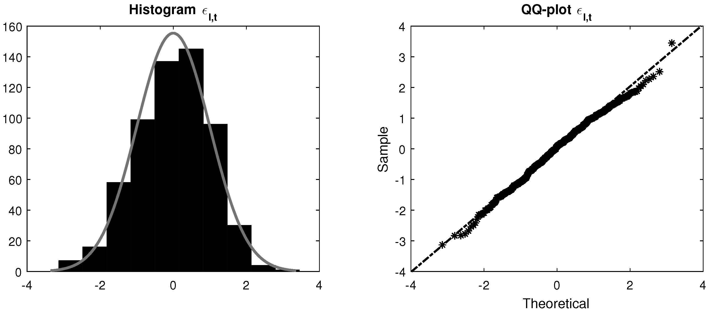
Figure 4.
Probability of deflation for 1-, 2-, 3-, and 5-year horizons. Parameters of Table 4 and Panel C of Table 5 were used to filter the real inflation rate, the expected inflation rate, and the conditional variance. Then, the latent variables were utilized to compute time series of probabilities. Deflation corresponds to an annualized average inflation that is less than 0% for a given time horizon, under the physical measure . The grey-shaded region highlights the NBER-dated recession.
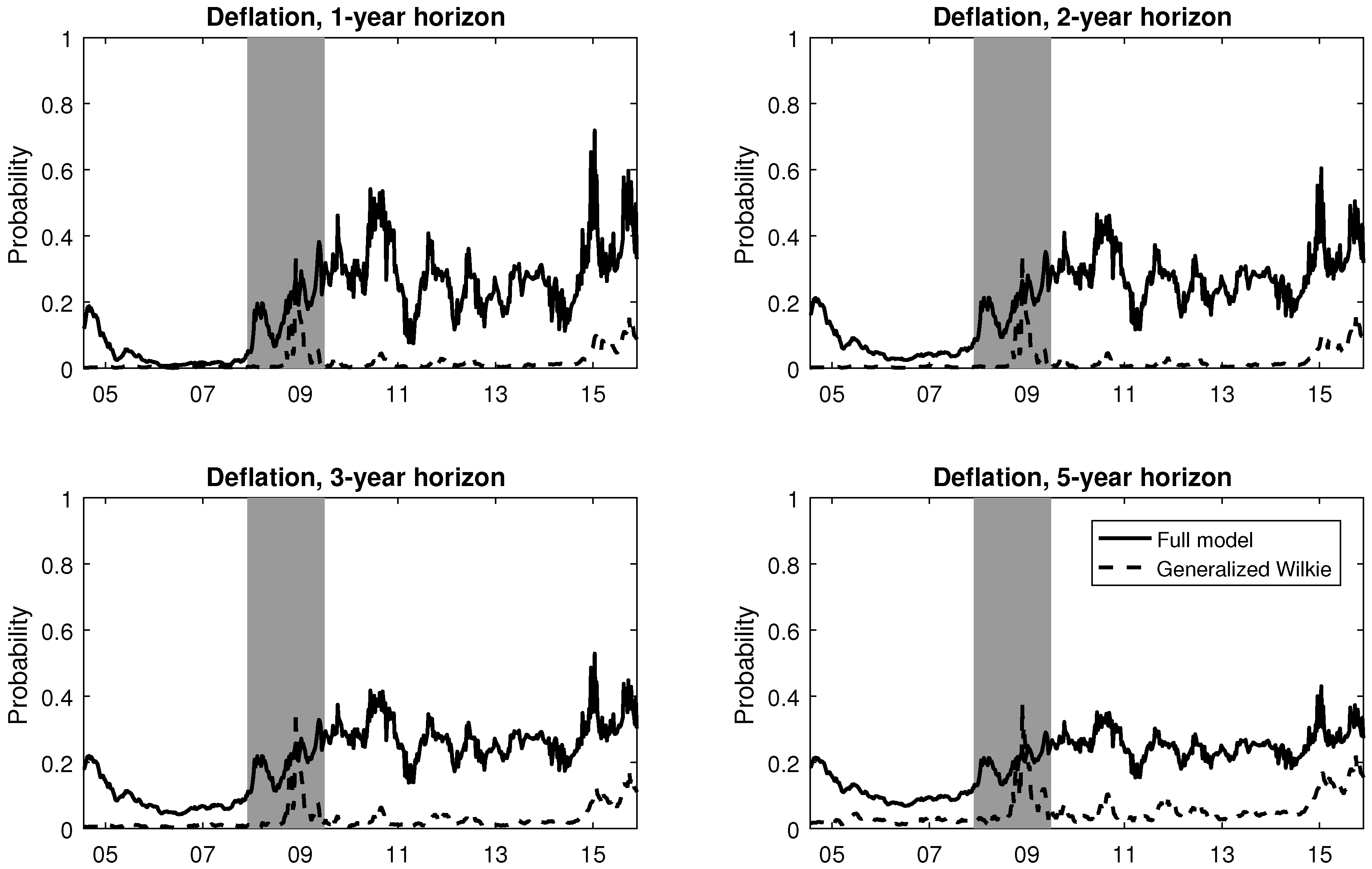
Figure 5.
Histograms of life insurer’s future payments on 5 February 2014, in present value. Portfolio present values are simulated using the method presented in Section 5 for four different inflation assumptions: full inflation (top left panel), anticipated inflation (top right panel), nominal interest rate (bottom left panel), and generalized Wilkie model (bottom right panel). Then, histograms are plotted and risk-measures are calculated. Values are reported in millions. CTE refers to the conditional tail expectation and VaR means value-at-risk.

Figure 6.
Risk-measures for the life insurer’s future payments, in present value. Values-at-risk and conditional tail expectations are computed under four inflation assumptions: full model, anticipated inflation, nominal interest rate, and the generalized Wilkie model. The confidence level is set at 95%. Values are reported in millions. Computations are done using the parameters of Table 4 and Table 5. Real interest rate () and expected inflation rates () displayed in the figure are in percentages (annualized). The conditional variance is set to its unconditional average w (i.e., ). Monte Carlo simulations are used to compute the risk measures. A sample of observations are generated to compute each measure.

Figure 7.
Time series of risk measures for the life insurer’s future payments, in present value. Values-at-risk and conditional tail expectations were computed under four inflation assumptions: full model, anticipated inflation, nominal interest rate, and the generalized Wilkie model. The confidence level is set at 95%. Values are reported in millions. Computations were done using the parameters of Table 4 and Table 5. Monte Carlo simulations were used to compute the risk measures. A sample of observations were generated to compute each measure. The grey-shaded region highlights the NBER-dated recession.

Figure 8.
Time series of risk-measures for the life insurer’s future payments, in present value. Values-at-risk and conditional tail expectations were computed under two inflation assumptions: the full model and the generalized Wilkie model. The confidence level is set at 95%. Values are reported in millions. Computations were done using the parameters of Table 4 and Table 5. Monte Carlo simulations were used to compute the risk measures. A sample of observations were generated to compute each measure. The grey-shaded region highlights the NBER-dated recession.


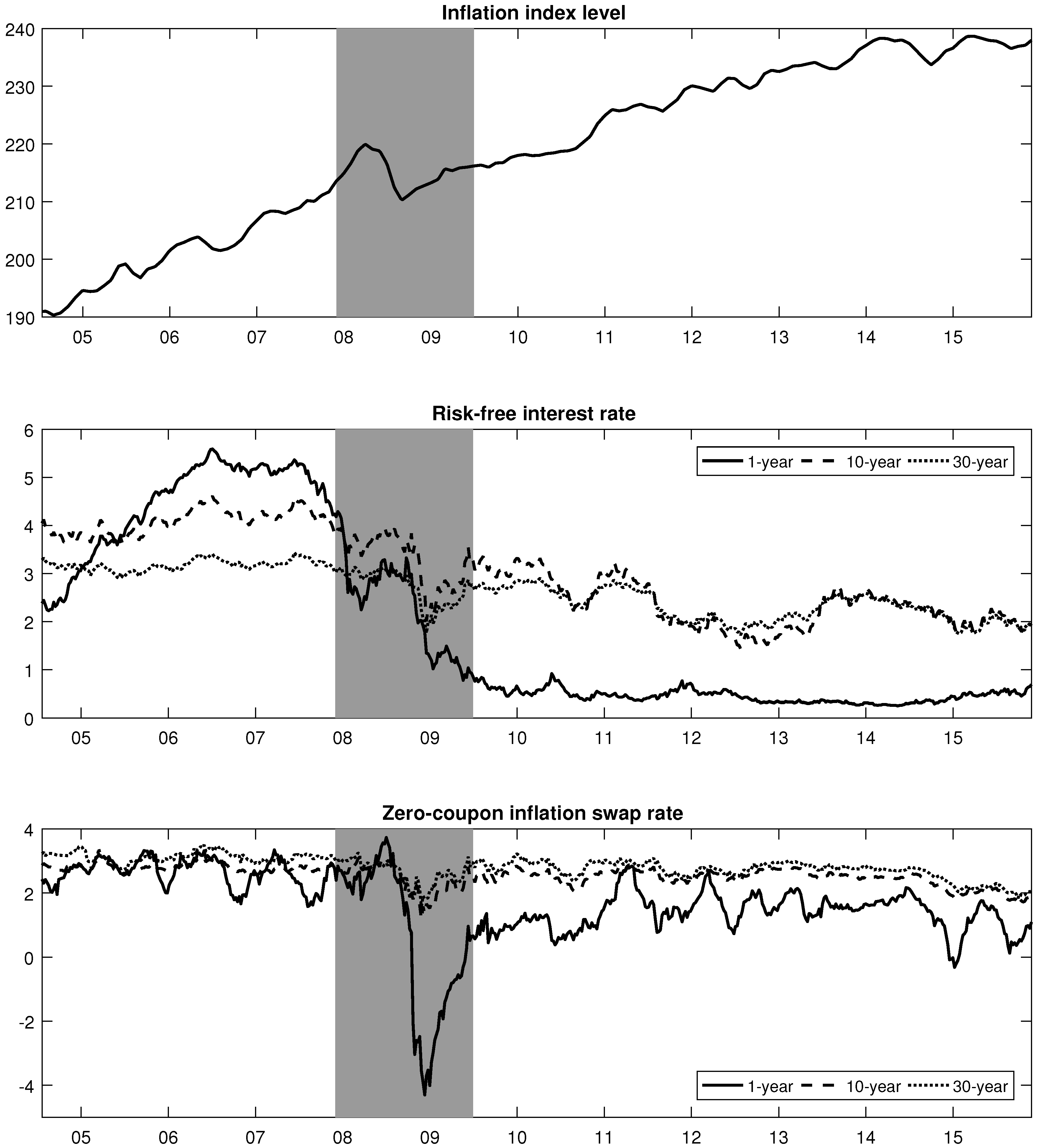
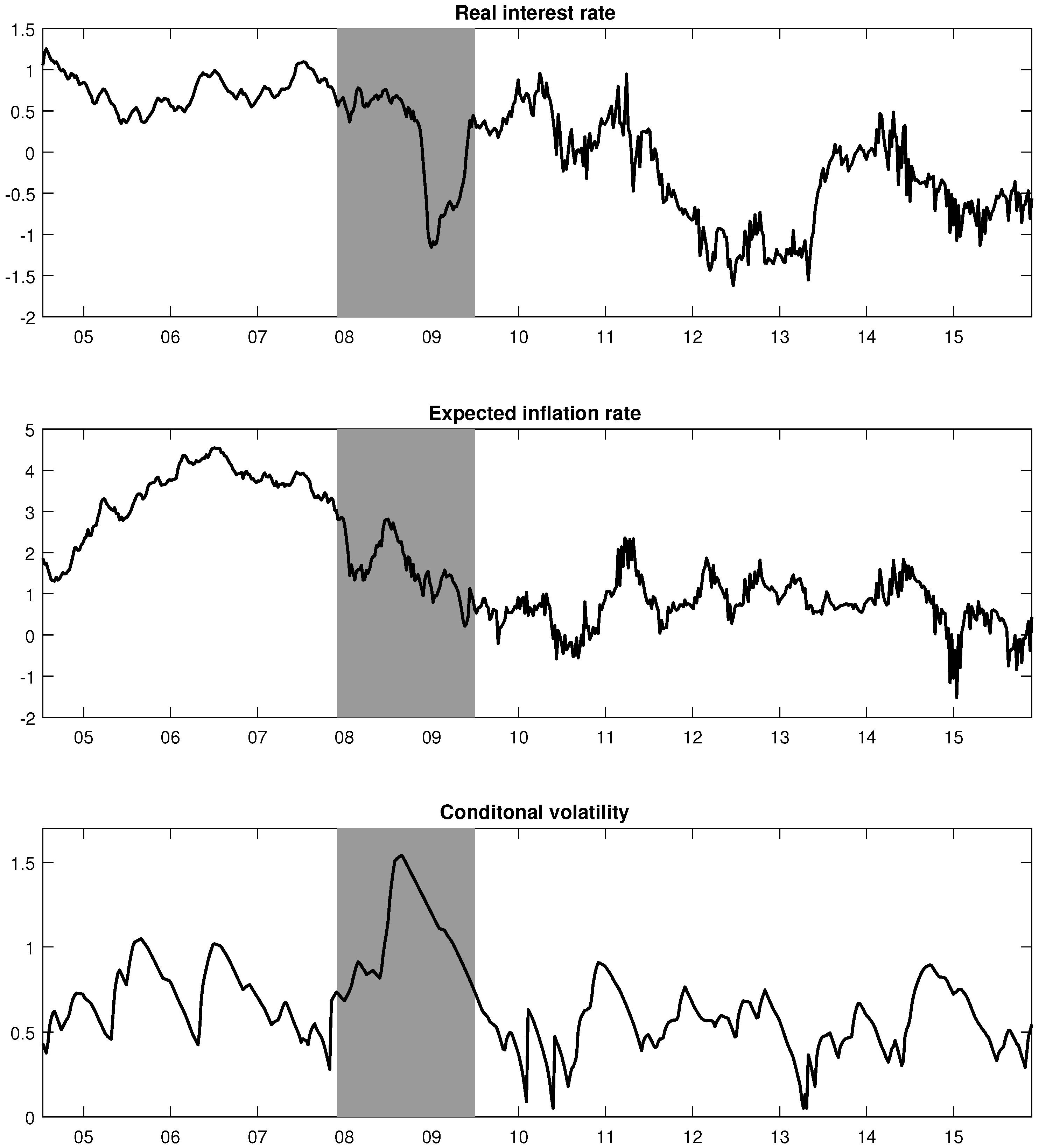
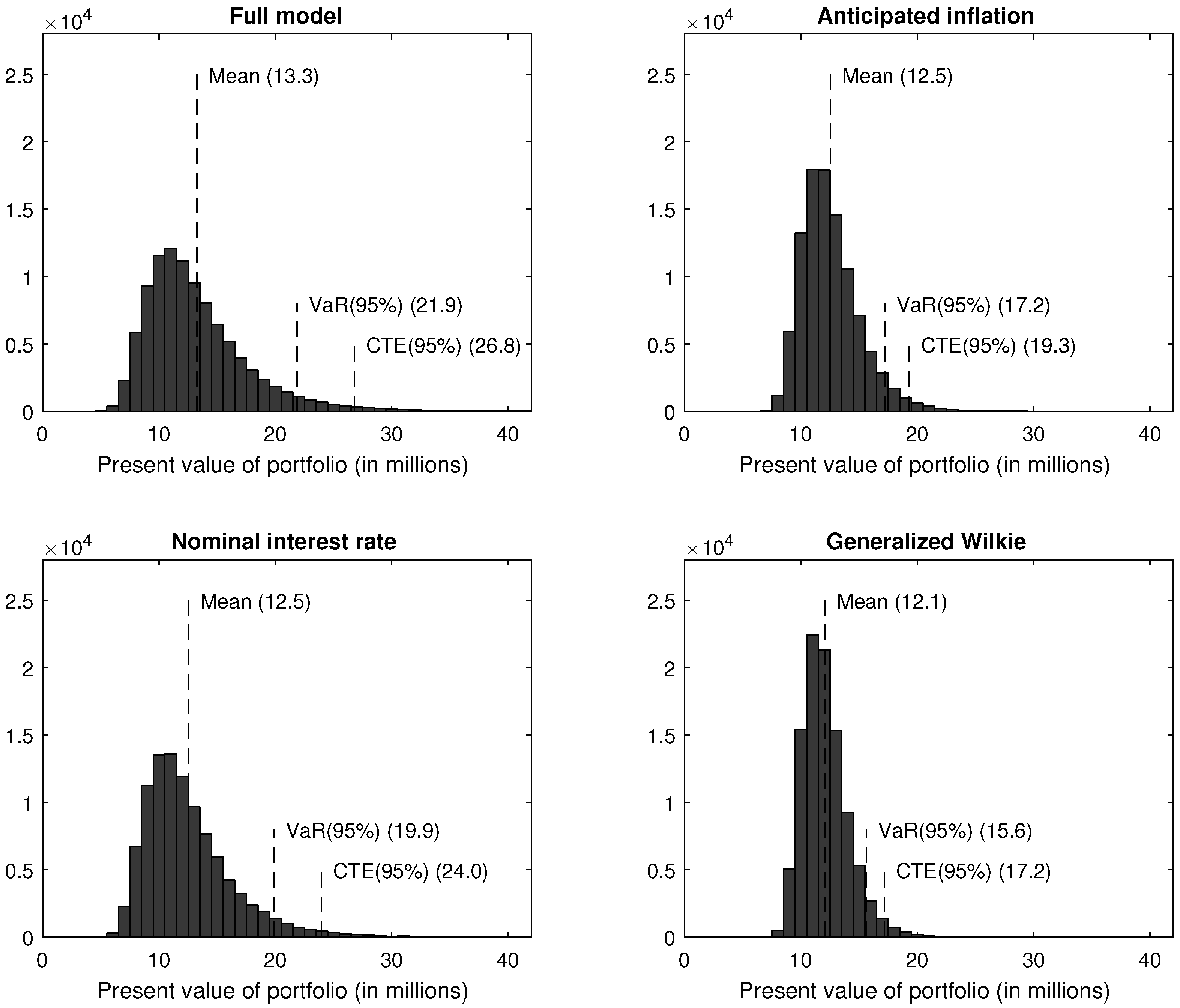
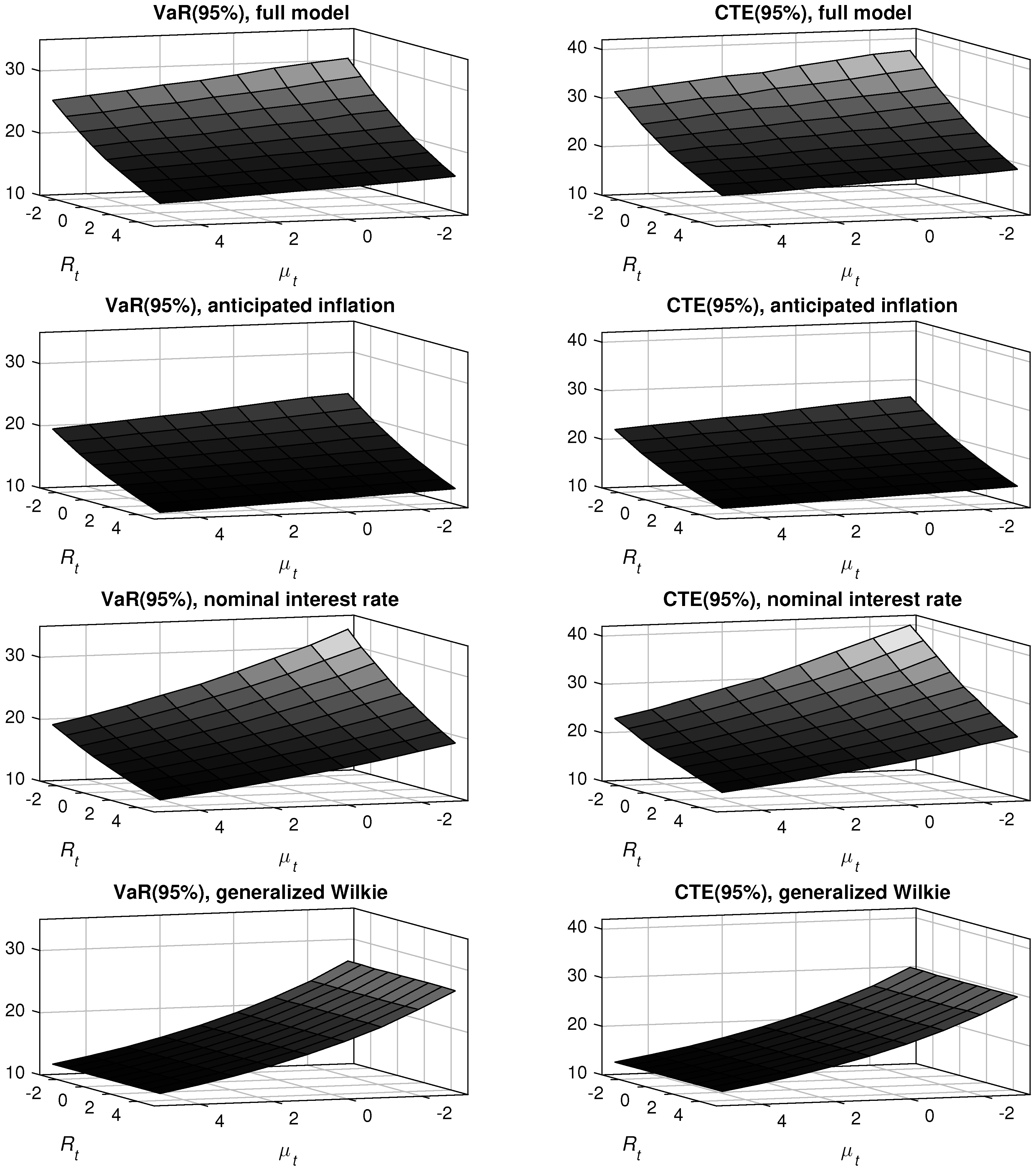
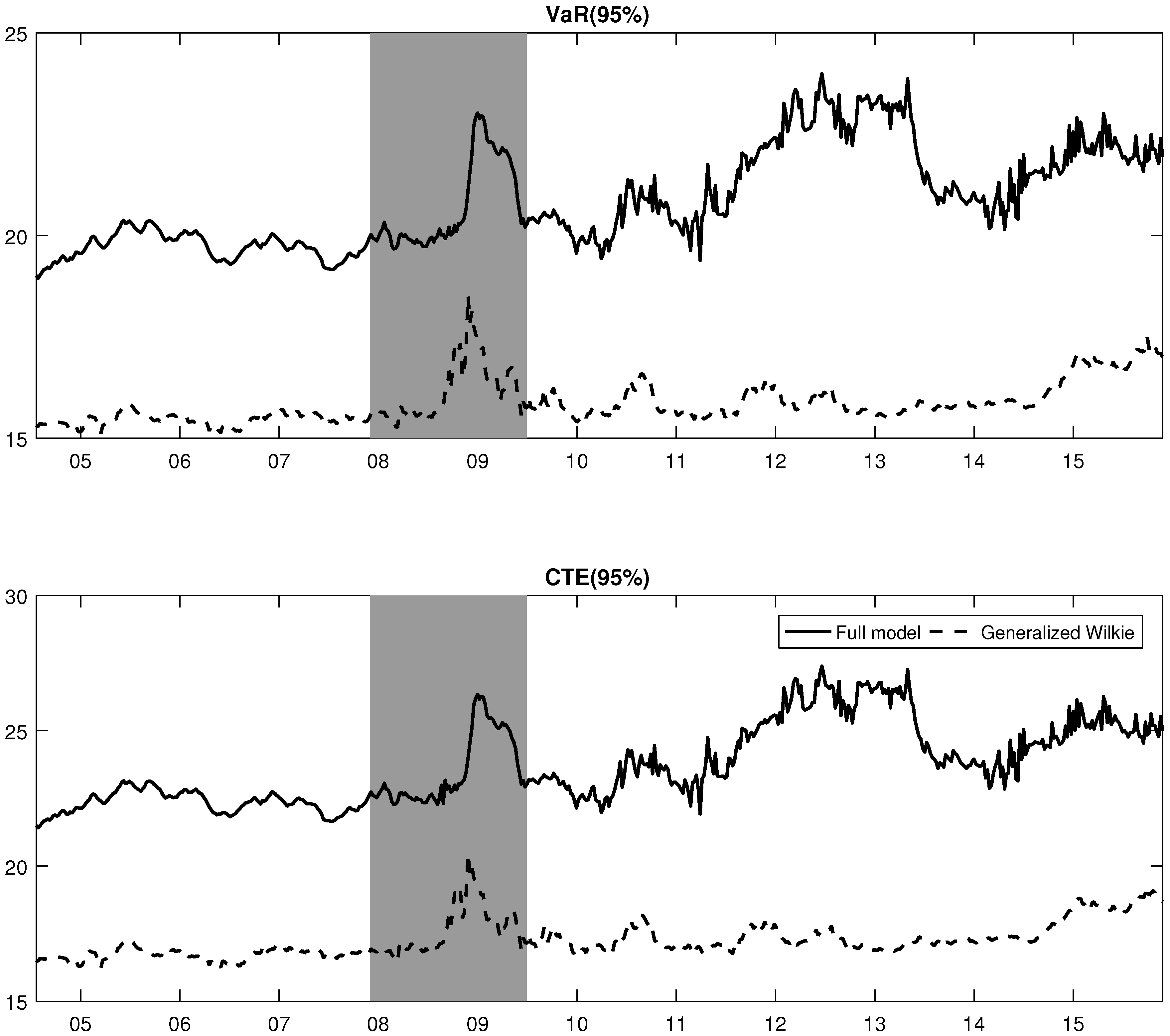
| Dynamics | Parameter | Interpretation |
|---|---|---|
| Real interest rate | θ | Unconditional level of real interest rate under |
| Unconditional level of real interest rate under | ||
| κ | Speed of mean reversion | |
| σ | Volatility of the real interest rate innovations | |
| Initial real interest rate | ||
| ρ | Correlation coefficient between real interest rate and | |
| expected inflation innovations | ||
| Expected inflation | ν | Unconditional level of expected inflation under |
| Unconditional level of expected inflation under | ||
| β | Speed of mean reversion | |
| γ | Volatility of the expected inflation innovations | |
| Initial expected inflation rate | ||
| Conditional variance | w | Unconditional level of variance |
| a | ARCH parameter | |
| b | GARCH parameter (i.e., persistence) | |
| c | Asymmetry parameter | |
| Initial variance level | ||
| Error standard deviations | Standard deviation of bonds | |
| Standard deviation of swaps | ||
| Homoskedastic standard deviation of implied volatilities | ||
| Adjustment parameter for option maturity | ||
| Adjustment parameter for option strike |
ARCH means autoregressive conditional heteroskedasticity. GARCH stands for generalized autoregressive conditional heteroskedasticity.
| Panel A: Risk-Free Interest Rates | ||||||||
| Maturity | Mean | SD | Min | Median | Max | |||
| 1/12 | 1.655 | 1.965 | 0.148 | 0.202 | 0.263 | 3.114 | 5.805 | 593 |
| 1/6 | 1.731 | 1.955 | 0.189 | 0.242 | 0.348 | 3.172 | 5.723 | 593 |
| 1/4 | 1.793 | 1.943 | 0.223 | 0.279 | 0.468 | 3.231 | 5.679 | 593 |
| 1/6 | 1.948 | 1.874 | 0.320 | 0.443 | 0.734 | 3.388 | 5.540 | 593 |
| 1 | 1.886 | 1.873 | 0.250 | 0.419 | 0.618 | 3.573 | 5.591 | 593 |
| 2 | 2.048 | 1.709 | 0.339 | 0.624 | 1.117 | 3.669 | 5.425 | 593 |
| 3 | 2.255 | 1.563 | 0.427 | 0.937 | 1.639 | 3.807 | 5.279 | 593 |
| 4 | 2.450 | 1.426 | 0.554 | 1.265 | 1.998 | 3.824 | 5.167 | 593 |
| 5 | 2.615 | 1.300 | 0.717 | 1.546 | 2.284 | 3.862 | 5.062 | 593 |
| 7 | 2.843 | 1.097 | 1.088 | 1.907 | 2.665 | 3.862 | 4.868 | 593 |
| 10 | 2.989 | 0.899 | 1.432 | 2.165 | 2.927 | 3.832 | 4.606 | 593 |
| 30 | 2.620 | 0.481 | 1.719 | 2.166 | 2.660 | 3.090 | 3.436 | 593 |
| Panel B: Inflation Swap Rates | ||||||||
| Maturity | Mean | SD | Min | Median | Max | |||
| 1 | 1.652 | 1.217 | −4.301 | 1.170 | 1.740 | 2.520 | 3.732 | 593 |
| 2 | 1.856 | 0.962 | −3.605 | 1.449 | 1.878 | 2.536 | 3.460 | 593 |
| 3 | 2.018 | 0.757 | −2.047 | 1.672 | 2.033 | 2.583 | 3.335 | 593 |
| 4 | 2.145 | 0.620 | −1.112 | 1.811 | 2.157 | 2.605 | 3.280 | 593 |
| 5 | 2.249 | 0.535 | −0.478 | 1.946 | 2.295 | 2.640 | 3.271 | 593 |
| 6 | 2.329 | 0.467 | 0.218 | 2.092 | 2.396 | 2.651 | 3.249 | 593 |
| 7 | 2.397 | 0.417 | 0.504 | 2.207 | 2.474 | 2.687 | 3.160 | 593 |
| 8 | 2.454 | 0.381 | 0.768 | 2.306 | 2.537 | 2.713 | 3.195 | 593 |
| 9 | 2.503 | 0.347 | 0.988 | 2.364 | 2.575 | 2.733 | 3.096 | 593 |
| 10 | 2.549 | 0.321 | 1.173 | 2.429 | 2.621 | 2.760 | 3.110 | 593 |
| 12 | 2.606 | 0.308 | 1.346 | 2.488 | 2.673 | 2.811 | 3.130 | 593 |
| 15 | 2.674 | 0.310 | 1.336 | 2.540 | 2.742 | 2.883 | 3.300 | 593 |
| 20 | 2.733 | 0.321 | 1.267 | 2.595 | 2.808 | 2.950 | 3.360 | 593 |
| 25 | 2.773 | 0.333 | 1.414 | 2.637 | 2.845 | 2.991 | 3.390 | 593 |
| 30 | 2.815 | 0.342 | 1.573 | 2.677 | 2.877 | 3.035 | 3.500 | 593 |
Inflation swap rates are expressed in percentage and maturities in years. Zero-coupon inflation swap rates are extracted from the Bloomberg system from July 2004 to December 2015. The risk-free interest rate is proxied by both LIBOR rates (for maturities less than 1 year) and swap rates (for maturities more than or equal to 1 year). The LIBOR and interest swap rates are collected via FRED from July 2004 to December 2015. The mean, standard deviation (SD), the minimum (Min), the first quartile (), the median, the third quartile (), the maximum (Max), and the number of observations (N) are computed across time for each tenor.
| Maturity | Mean | N | |||||||
|---|---|---|---|---|---|---|---|---|---|
| 1 | 1.775 | 1.586 | 1.361 | 1.299 | 1.382 | 1.695 | 2.028 | 1.589 | 2868 |
| 2 | 2.616 | 2.289 | 1.896 | 1.804 | 1.949 | 2.326 | 2.617 | 2.214 | 2916 |
| 3 | 3.166 | 2.766 | 2.236 | 2.102 | 2.251 | 2.723 | 3.192 | 2.633 | 2862 |
| 5 | 4.043 | 3.505 | 2.757 | 2.584 | 2.745 | 3.325 | 3.882 | 3.263 | 2465 |
| 7 | 4.811 | 4.192 | 3.263 | 2.920 | 3.072 | 3.863 | 4.515 | 3.805 | 2212 |
| 10 | 5.727 | 5.059 | 4.249 | 3.225 | 3.451 | 4.459 | 5.250 | 4.489 | 2085 |
| 15 | 6.682 | 5.852 | 4.954 | 3.667 | 3.422 | 4.913 | 5.863 | 5.050 | 1856 |
| 20 | 7.453 | 6.416 | 5.312 | 3.787 | 3.170 | 5.145 | 6.349 | 5.376 | 1807 |
| 30 | 8.656 | 7.290 | 5.860 | 3.990 | 3.005 | 5.525 | 7.108 | 5.919 | 1626 |
Inflation option implied volatilities and strikes are expressed in percentage, and maturities in years. The zero-coupon inflation cap and floor prices are collected via the Bloomberg system from October 2009 to December 2015. The inflation cap and floor implied volatility are computed by inverting Black and Scholes’ pricing formula. The average implied volatilities and the number of observations (N) are computed across time and strikes for each maturity.
Table 4.
Parameter estimates and standard errors for the full model when using CPI-U levels, nominal risk-free bond prices, inflation swap prices, and option implied volatilities.
| Real Interest Rate | Expected Inflation | Conditional Variance | Error Standard Deviations | ||||
|---|---|---|---|---|---|---|---|
| θ | 3.54 | ν | 3.48 | w | 9.13 | 8.36 | |
| (4.34) | (1.98) | (1.26) | (2.32) | ||||
| 3.24 | 7.05 | a | 6.43 | 1.89 | |||
| (8.70) | (9.45) | (1.91) | (5.00) | ||||
| κ | 9.99 | β | 9.92 | b | 9.87 | 4.78 | |
| (1.44) | (7.56) | (3.22) | (2.99) | ||||
| σ | 3.64 | γ | 7.55 | c | 1.12 | 1.25 | |
| (9.04) | (5.20) | (2.72) | (3.68) | ||||
| 2.03 | 3.58 | 3.61 | 1.35 | ||||
| (2.24) | (7.53) | (1.69) | (3.14) | ||||
| ρ | 7.08 | ||||||
| (1.14) | |||||||
Parameters are estimated using the UKF with CPI-U levels, nominal risk-free bond prices and inflation swap prices only from July 2004 to December 2015, as well as option implied volatilities from October 2009 to December 2015. The log-likelihood function is maximized using multiple simplex search method optimizations (fminsearch in Matlab). Robust standard errors (in parentheses) are calculated from the outer product of the gradient at the optimum parameter value. For more details on this technique, see Appendix B.5 of Rémillard [33].
| Panel A: Nominal Interest Rate Model | |||||||
| Nominal Interest Rate | Expected Inflation | Conditional Variance | Error Standard Deviations | ||||
| θ | 7.85 | ν | - | w | - | 1.48 | |
| (1.81) | - | - | (2.53) | ||||
| 1.02 | - | a | - | - | |||
| (6.22) | - | - | - | ||||
| κ | 9.98 | β | - | b | - | - | |
| (2.27) | - | - | - | ||||
| σ | 6.42 | γ | - | c | - | - | |
| (6.06) | - | - | - | ||||
| 7.60 | - | - | - | ||||
| (1.60) | - | - | - | ||||
| ρ | - | ||||||
| - | |||||||
| Panel B: Generalized Wilkie’s [9] (GW) Model | |||||||
| Real Interest Rate | Expected Inflation | Conditional Variance | Error Standard Deviations | ||||
| θ | - | ν | 1.26 | w | 9.32 | - | |
| - | (2.33) | (1.41) | - | ||||
| - | 1.40 | a | - | 1.56 | |||
| - | (7.57) | - | (2.44) | ||||
| κ | - | β | 1.00 | b | - | - | |
| - | (6.33) | - | - | ||||
| σ | - | γ | 2.34 | c | - | - | |
| - | (3.90) | - | - | ||||
| - | 5.04 | - | - | ||||
| - | (2.60) | - | - | ||||
| ρ | - | ||||||
| - | |||||||
Parameters of Panel A (Nominal interest rate model) are estimated using the UKF with nominal risk-free bond prices from July 2004 to December 2015. Parameters of Panel B (Generalized Wilkie) are estimated using the UKF with CPI-U levels and inflation swap prices from July 2004 to December 2015. The log-likelihood function is maximized using multiple simplex search method optimizations (fminsearch in Matlab). Robust standard errors (in parentheses) are calculated from the outer product of the gradient at the optimum parameter value. For more details on this technique, see Appendix B.5 of Rémillard [33].
© 2016 by the author; licensee MDPI, Basel, Switzerland. This article is an open access article distributed under the terms and conditions of the Creative Commons Attribution (CC-BY) license (http://creativecommons.org/licenses/by/4.0/).
Share and Cite
MDPI and ACS Style
Bégin, J.-F. Deflation Risk and Implications for Life Insurers. Risks 2016, 4, 46. https://doi.org/10.3390/risks4040046
AMA Style
Bégin J-F. Deflation Risk and Implications for Life Insurers. Risks. 2016; 4(4):46. https://doi.org/10.3390/risks4040046
Chicago/Turabian StyleBégin, Jean-François. 2016. "Deflation Risk and Implications for Life Insurers" Risks 4, no. 4: 46. https://doi.org/10.3390/risks4040046
Note that from the first issue of 2016, this journal uses article numbers instead of page numbers. See further details here.