Risk Minimization for Insurance Products via F-Doubly Stochastic Markov Chains

Abstract

We study risk-minimization for a large class of insurance contracts. Given that the individual progress in time of visiting an insurance policy’s states follows an $\mathbb{F}$-doubly stochastic Markov chain, we describe different state-dependent types of insurance benefits. These cover single payments at maturity, annuity-type payments and payments at the time of a transition. Based on the intensity of the $\mathbb{F}$-doubly stochastic Markov chain, we provide the Galtchouk-Kunita-Watanabe decomposition for a general insurance contract and specify risk-minimizing strategies in a Brownian financial market setting. The results are further illustrated explicitly within an affine structure for the intensity.

1. Introduction

The management of an insurance portfolio’s risk is one of the core challenges in actuarial science. While the classic form of risk mitigation is based on reinsurance contracts, in some cases it is also possible to hedge claim payments by appropriately trading in different assets. This particularly applies if the assets are correlated to the insurance contract’s benefits or their (conditional) probability of occurrence. Practical examples in this direction are unit-linked life insurance products, where benefits depend on the performance of the assets, or unemployment insurance products, where the occurrence of a claim payment may depend to some extend on economic and financial conditions of the markets. Moreover, there is an ongoing discussion about the introduction of so called longevity bonds which would establish the possibility for life insurance companies and pension funds to hedge parts of their longevity risk, see [1,2] or [3]. Due to their unsystematic risk part, most insurance claims are not hedgeable completely through a self-financing trading strategy which particularly means that a hybrid market, consisting among others of financial and insurance markets, is incomplete. A reasonable method for optimally choosing an investment strategy is then important to cover at least parts of the risk.

In the present paper we choose the risk-minimization approach and determine hedging strategies in the sense of this criterion for insurance contracts in a very general setting. This quadratic hedging approach bases on the results in [4] for European type payments and to [5] for payment processes. In most cases, the risk-minimizing strategies can be derived from the well known Galtchouk-Kunita-Watanabe (GKW-) decomposition, see [6] or [7].

Similar to the works of [5,8] or [9,10,11], we describe an insured person’s progress of sojourning different states of an insurance policy as a right continuous stochastic process with finite state space $\mathcal{K}=\{1,...,N\}$, 1 being a.s. the initial state. More specifically, we adopt the class of $\mathbb{F}$-doubly stochastic Markov chains as introduced in [12], see Appendix A and the comments therein. This family of processes has several properties which make them very suitable for applications in credit risk and insurance market modeling. Being a sub-class of $\mathbb{F}$-conditional Markov chains, they extend the classic notion of Markov chains by including a reference filtration $\mathbb{F}$ which in our case represents additional market information. In this way we are able to take in consideration the influence of external risk factors and economic and financial conditions on transition probabilities of an insured person’s progress. In particular, $\mathbb{F}$-doubly stochastic Markov chains behave like time inhomogeneous Markov chains, if we know all the information concerning the underlying risk factors. This corresponds to the intuition that the transition probabilities would be completely specified, if we would dispose of full knowledge on the underlying economic and financial situation.

Another important feature is that, if we specify the information as given by the filtration $\mathbb{G}:={\mathbb{F}}^X\vee \mathbb{F}$, where ${\mathbb{F}}^X$ is the natural filtration of the $\mathbb{F}$-doubly stochastic Markov chain X, then we have that predictable representation theorems and the so-called hypothesis (H) 1, or immersion property, hold. These properties play a fundamental role in order to compute the optimal strategy for insurance contracts according to the risk-minimization method.

Furthermore, $\mathbb{F}$-doubly stochastic Markov chains may admit matrix-valued stochastic intensity processes. This allows to investigate more flexible models compared to the results e.g., in Møller [5] where a (classical) Markov chain with deterministic intensity matrix function is considered. One further advantage is that $\mathbb{F}$-doubly stochastic Markov chains with intensity are fully characterized by some martingale properties, which can be used for the estimation of the underlying intensity processes, see Biagini et al. [13].

Well known examples of $\mathbb{F}$-doubly stochastic Markov chains are reduced form or intensity based models in the case that hypothesis (H) is satisfied. Here, the state space consists of two states with the second state being absorbing such that there can only occur one transition in time. There exist many works on quadratic hedging for these models particularly in the context of credit risk or life insurance theory, see e.g., [1,2,14,15,16,17,18,19] or [20]. In particular, the present paper extends these works to a multi-state framework where several subsequent transitions, driven by $\mathbb{F}$-adapted stochastic intensity processes, are considered. This general setting allows to investigate a larger class of insurance contracts, e.g., income protection insurance contracts with the states “healthy”, “sick” and “deceased”, and to include the influence of market conditions and external risk factors on the insured person’s progress.

Given an $\mathbb{F}$-doubly stochastic Markov chain, we propose a general insurance contract, defined by three different types of insurance benefits: state-dependent payments at maturity, state-dependent annuity-type payments, and (transition-dependent) payments at the time of a transition from one state to another. This definition covers a large set of currently adopted insurance policies. In particular, we illustrate the definitions for pure endowment, term insurance, general life annuity and payment protection insurance contracts. Similar to the results in [21], who applied $\mathbb{F}$-doubly stochastic Markov chains in the context of hedging rating-sensitive financial claims, we obtain the GKW-decomposition for the payment process of general insurance contracts with respect to a particular $\mathbb{F}$-martingale. In this context, we generalize and complement the proofs in [21] in order to adapt the results for the risk-minimization approach which is not investigated there.

Given that the reference information $\mathbb{F}$ is generated by an N-dimensional Brownian motion $\mathbf{W}$, we then introduce a financial market model, driven by $\mathbf{W}$. In this setting we infer risk-minimizing hedging strategies for insurance contracts with deterministic payment structure with respect to the assets on the financial market. Similarly to the work in [2] we then assume a general affine structure for the intensity of the underlying $\mathbb{F}$-doubly stochastic Markov chain and obtain explicit formulas for the strategies and their residual risk processes. We apply these results in the specific example of an income protection insurance, where we assume that the intensities follow a (multi-dimensional) Ornstein-Uhlenbeck process. We discuss the resulting expected cumulative payment, which may be considered as a fair premium in the interpretation of [22,23], as a function of the time horizon, the payment amounts and the underlying interest rates.

The paper is organized as follows. In Section 2 we introduce the notion of general insurance contracts and discuss several examples. In Section 3 we prove our main results for the risk minimization of this kind of contracts in full generality. The risk minimizing strategies are then further illustrated within a general affine specification for the intensities and in a numerical example in an Ornstein-Uhlenbeck framework. We conclude the paper with Appendix A and Appendix B, where we summarize important results and concepts of risk-minimization and $\mathbb{F}$-doubly stochastic Markov chains for the reader’s convenience.

2. General Insurance Contracts

We now introduce the notion of general insurance contracts and provide some well known examples of actuarial practice.

In the same notation as in Appendix A, let $(\mathsf{\Omega },\mathcal{G},\mathbb{G},\mathbb{P})$ be a filtered probability space with $\mathbb{G}={\mathbb{F}}^X\vee \mathbb{F}$ for some $\mathbb{F}$-doubly stochastic Markov chain X with state space $\mathcal{K}=\{1,...,N\}$. We assume $\mathbb{P}(X_0=1)=1$. The following definition of general insurance contracts is based on the definitions for payment processes on rating sensitive claims as given e.g., in [21] or [20]. The definition also covers the concepts of insurance contracts as given in [5] or [9].

Definition 1.

A general insurance contract is given by the quadruple $(X;\mathit{A};\mathit{Y};\mathit{Z})$, where $X={\left(X_t\right)}_{t\in [0,T]}$ is an $\mathbb{F}$-doubly stochastic Markov chain, $\mathit{A}={(A_t^1,...,A_t^N)}_{t\in [0,T]}$ is an $\mathbb{F}$-adapted, N-dimensional process of finite variation, $\mathit{Y}=(Y^1,...,Y^N)$ is an ${\mathcal{F}}_T$-measurable, N-dimensional random vector, and $\mathit{Z}={\left({\mathit{Z}}_t\right)}_{t\in [0,T]}$ with ${\mathbf{Z}}_t={\left[Z_t^{j,k}\right]}_{j,k\in \mathcal{K}}$ is an $\mathbb{F}$-adapted, $N\times N$-dimensional process with zeros on the diagonal.

The different elements of a general insurance product’s quadruple are interpreted as follows. The process X is the insured person’s progress in time of sojourning in the states $j\in \mathcal{K}$, considered by the insurance policy. The N-dimensional process $\mathbf{A}$ characterizes the cumulative state-dependent payment streams which are continuously paid up to maturity. For example, one can take ${\mathbf{A}}_t={\mathbf{C}}_t-{\mathbf{P}}_t$, $t\in [0,T]$ with ${\mathbf{C}}_t={(C_t^1,...C_t^N)}^{⊺}$ representing the cumulative state-dependent claim payments (e.g., annuities) and ${\mathbf{P}}_t=(P_t^1,...,P_t^N)$ the cumulative state-dependent insurance premiums up to maturity. Both processes, $\mathbf{P}$ and $\mathbf{C}$ are then taken to be $\mathbb{F}$-adapted, càdlàg and increasing. The vector $\mathbf{Y}$ characterizes state-dependent “extra” claim payments at maturity T and the process $\mathbf{Z}$ the “immediate” claim payments at the transition times from one state to another.

For every general insurance contract $(X;\mathbf{A};\mathbf{Y};\mathbf{Z})$ the cumulative payment process $D={\left(D_t\right)}_{t\in [0,T]}$ is given by

$$\begin{array}{ccc}{D}_t:\hfill & =\hfill & {\mathbf{Y}}^{⊺}{\mathbf{H}}_T{\mathbb{1}}_{\{t=T\}}+{\int }_{[0,t]}{\mathbf{H}}_s^{⊺}d{\mathbf{A}}_s+{\int }_{]0,t]}{\left({\mathbf{Z}}_s^{⊺}{\mathbf{H}}_{s-}\right)}^{⊺}d{\mathbf{H}}_s\hfill \\ & =\hfill & {\sum }_{j=1}^N\left(Y^j{H}_T^j{\mathbb{1}}_{\{t=T\}}+{\int }_{[0,t]}{H}_s^{j}d{A}_s^j+{\sum }_{\begin{array}{c}k=1\\ k\ne j\end{array}}^N{\int }_{]0,t]}{Z}_s^{j,k}d{N}_s^{jk}\right)\hfill \end{array}$$

(1)

with $H_t^j,j\in \mathcal{K},$ as defined in Equation (A7) and counting processes $N_t^{jk}$ from Equation (A8). Note that D is of finite variation. We now provide some well known examples of insurance contracts.

Example 1.

A pure endowment is an insurance contract which guarantees to the insured person some fixed payment if she is alive at maturity. For the sake of simplicity, we only consider the payment to be equal to 1.

We set $\mathcal{K}=\{1,2\}$ with 1 being the state “alive” and 2 the absorbing state “deceased”. A pure endowment contract is then given as the quadruple $(X;0;{(1,0)}^{⊺};0)$ or $(X;-\mathit{P};{(0,1)}^{⊺};0)$ if premium payments are considered, respectively.

Example 2.

A term insurance is an insurance contract which guarantees the heirs of an insured person some fixed payment at the time of decease. For the sake of simplicity, we only consider the payment to be equal to 1.

Again, we set $\mathcal{K}=\{1,2\}$ with 1 being the state “alive” and 2 the absorbing state “deceased”. Then a term insurance contract is given as the quadruple $(X;0;0;\mathit{Z})$ or $(X;-\mathit{P};0;\mathit{Z})$ if premium payments are considered, respectively, with $\mathit{Z}:=\left(\begin{array}{cc}0& 1\\ 0& 0\end{array}\right)$.

Example 3.

A general annuity as defined in [2] is an insurance contract which guarantees the insured person an $\mathbb{F}$-progressively measurable, non-negative continuous rate payment ${\left(c_t\right)}_{t\in [0,T]}$ as long as she is alive. The state space is again $\mathcal{K}=\{1,2\}$ with 1 being the state “alive” and 2 the absorbing state “deceased”. Then a general annuity contract is given as the quadruple $(X;{\left({\int }_{]0,t]}{c}_{s}ds,0\right)}_{t\in [0,T]}^{⊺};0;0)$ or $(X;{\left({\int }_{]0,t]}{c}_{s}ds,0\right)}_{t\in [0,T]}^{⊺}-\mathit{P};0;0)$ if premium payments are considered, respectively.

Example 4.

A payment protection insurance (PPI) is an insurance contract which is usually offered as an add-on product to some payment obligations, e.g., a loan. In the case of an insured event, the insurance company takes over the respective instalments of the payment obligation for the insured person or her heirs. Generally, the insured events are “disability”, “unemployment” and “decease”. Hence, the state space for PPI products is given as $\mathcal{K}=\{1,2,3,4\}$ with “2” being the state “disabled”, “3” the state “unemployed”, “4” the absorbing state “deceased” and “1” the state where no insured event is present.

Then a PPI contract is given as the quadruple $(X;{(0,C_t^2,C_t^3,C_t^4)}_{t\in [0,T]}^{⊺};{(0,Y,Y,Y)}^{⊺};0)$ or $(X;{(0,C_t^2,C_t^3,C_t^4)}_{t\in [0,T]}^{⊺}-\mathit{P};{(0,Y,Y,Y)}^{⊺};0)$ if premium payments are considered, respectively.

As the underlying payment obligation usually stipulates fixed instalments $c_1,...,c_K$ at some given payment dates $0<T_1<...<T_K=T$, the processes $C_t^i$, $i=2,3,4$, are generally given as $C_t^i={\sum }_{j=1}^K{c}_j{\mathbb{1}}_{\{T_j\le t\}}$.

Moreover, some payment obligations also contain a so-called balloon rate B at the end of the contract, which has to be paid on top of the usual instalment. If there exists a balloon rate and it is insured, then we set $Y=B$, if there exists no balloon rate or it is not insured, then we set $Y=0$.

Remark 1.

(1) 

The extra claim payment could also be included in the continuous claim payments. For the reader’s convenience, however, we explicitly separate continuous and extra claim payments.

(2) 

The main concepts of premium payment are

-

a single premium P, where the complete price for the insurance contract is paid at its beginning. In this case, the vector $\mathit{P}$ would be given as $\mathit{P}={\left(P{\mathbb{1}}_{\{t\ge 0\}},P{\mathbb{1}}_{\{t\ge 0\}},...,P{\mathbb{1}}_{\{t\ge 0\}}\right)}_{t\in [0,T]}^{⊺}$.

-

periodically paid premiums. Here, the insurance price is paid according to periodically paid premiums $p_i$ at a priori specified dates $0=T_0<T_1<...<T_L\le T$. Moreover, some insurance policies consider premium freedoms which allow the insured person to intermit premium payments while sojourning (some) insured states. In this case, we have for each vector entry $P^i$, $i\in \{1,...,N\}$, of $\mathit{P}$

$$\begin{array}{c}\hfill P_t^i=\left\{\begin{array}{c}\sum _{j=1}^L{p}_j{\mathbb{1}}_{\{T_j\le t\}}\hfill \\ 0\hfill \end{array}\right.\end{array}$$

depending on whether state i is guarantees premium freedom or not.

3. Risk-Minimization for General Insurance Contracts

Aim of this paper is to provide the risk minimizing strategy for a general insurance contract by applying the approach presented in Appendix B. Risk minimization provides hedging strategies which perfectly replicate the claim. Since the market is incomplete, these strategies may not be self-financing and a readjustment (or cost) is needed to achieve perfect replication. According to this method we choose then the optimal strategy, i.e., the strategy with minimal cost.

For this sake, we first consider a general setting and then focus on a deterministic payment structure and an underlying market which is driven by some N-dimensional Brownian motion. These results are then further specified within a general affine setting for the different entries of the matrix-valued intensity.

3.1. Martingale Decomposition for Payment Processes of General Insurance Claims

We consider the payment process D in Equation (1). Let $S^0$ denote the market’s discounting factor, which will be further specified in Section 3.2. If ${\int }_{]0,T]}\frac{1}{S_u^0}d{\left|D\right|}_u<\infty$, we get by Equation (B1) that the discounted cumulative payment stream $\widehat{D}={\left({\widehat{D}}_t\right)}_{t\in [0,T]}$ is given as

$$\begin{array}{cc}{\widehat{D}}_t\hfill & =\frac{{\mathbf{Y}}^{⊺}{\mathbf{H}}_T}{S_T^0}{\mathbb{1}}_{\{t=T\}}+{\int }_{[0,t]}\frac{1}{S_s^0}{\mathbf{H}}_s^{⊺}d{\mathbf{A}}_s+{\int }_{]0,t]}\frac{1}{S_s^0}{\left({\mathbf{Z}}_s^{⊺}{\mathbf{H}}_{s-}\right)}^{⊺}d{\mathbf{H}}_s\hfill \\ & ={\sum }_{j=1}^N\left(\frac{Y^j{H}_T^j}{S_T^0}{\mathbb{1}}_{\{t=T\}}+{\int }_{[0,t]}\frac{1}{S_s^0}{H}_s^{j}d{A}_s^j+{\sum }_{\begin{array}{c}k=1\\ k\ne j\end{array}}^N{\int }_{]0,t]}\frac{1}{S_s^0}{Z}_s^{j,k}d{N}_s^{jk}\right)\hfill \end{array}$$

(2)

We further assume the underlying $\mathbb{F}$-doubly stochastic Markov chain X to admit an intensity $\mathsf{\Psi }={({[{\psi }_t^{j,k}]}_{j,k\in \mathcal{K}})}_{t\in [0,T]}$, as introduced in Definition A.5.

Assumption 2.

For every general insurance contract $(X;\mathit{A};\mathit{Y};\mathit{Z})$, let

$$\begin{array}{cc}& \mathbb{E}\left[{\left(\frac{Y^j}{S_T^0}\right)}^2\right]<\infty ,j\in \mathcal{K}\hfill \end{array}$$

(3)

$$\begin{array}{cc}& \underset{s\in [0,T]}{sup}\mathbb{E}\left[{\left({\int }_{[0,s]}\frac{1}{S_u^0}d{A}_u^j\right)}^2\right]<\infty ,j\in \mathcal{K}\hfill \end{array}$$

(4)

$$\begin{array}{cc}& \mathbb{E}\left[{\int }_{]0,T]}{\left({\int }_{[0,u]}\frac{1}{S_v^0}d{A}_v^j\right)}^2\left|{\psi }_{X_u,j}\right|du\right]<\infty ,j\in \mathcal{K}\hfill \end{array}$$

(5)

$$\begin{array}{cc}& \mathbb{E}\left[{\int }_{]0,T]}{\left(\frac{Z_u^{j,k}}{S_u^0}\right)}^2{\psi }_{j,k}\left(u\right)du\right]<\infty ,j,k\in \mathcal{K},j\ne k\hfill \end{array}$$

(6)

$$\begin{array}{cc}& \mathbb{E}\left[{\left({\int }_{]0,T]}\frac{Z_u^{j,k}}{S_u^0}{\psi }_{j,k}\left(u\right)du\right)}^2\right]<\infty ,j,k\in \mathcal{K},j\ne k\hfill \end{array}$$

(7)

where $H_t^j$, $t\in [0,T]$ is defined in Equation (A7).

Note that Equations (3), (4), (6) and (7) ensure that the discounted payment stream $\widehat{D}$ generated by the general insurance contract $(X;\mathbf{A};\mathbf{Y};\mathbf{Z})$ is square integrable.

We remark that the following Lemma is given similarly in [21] (Theorem $16.38$) under the assumption the local martingale $\mathbf{M}$, defined in Equation (A9), is square integrable and the processes $\mathbf{A}$ and $\mathbf{Z}$ are bounded. Here, we generalize their proof to the case where $\mathbf{A}$ and $\mathbf{Z}$ satisfy the conditions of Assumption 2.

For notational convenience, we introduce the process $\mathbf{G}={\left({\mathbf{G}}_t\right)}_{t\in [0,T]}={\left(G_t^1,...,G_t^N\right)}^{⊺}$ with

$$\begin{array}{c}\hfill G_t^j:={\left[{\mathbf{Z}}_t{\mathsf{\Psi }}_t^{⊺}\right]}_{j,j}=\sum _{\begin{array}{c}k=1\\ k\ne j\end{array}}^N{Z}_t^{j,k}{\psi }_{j,k}\left(t\right),j\in \mathcal{K},t\in [0,T]\end{array}$$

(8)

Lemma 3.

Let $(X;\mathit{A};\mathit{Y};\mathit{Z})$ be a general insurance contract, satisfying Assumption 2, then

$$\begin{array}{c}\mathbb{E}\left[\left.{\widehat{D}}_T-{\widehat{D}}_t\right|{\mathcal{G}}_t\right]=\sum _{j=1}^N\mathbb{E}\left[\frac{Y^j{H}_T^j}{S_T^0}+{\int }_{]t,T]}\frac{1}{S_u^0}{H}_u^{j}d{A}_u^j+\sum _{\begin{array}{c}k=1\\ k\ne j\end{array}}^N{\int }_{]t,T]}\frac{Z_u^{j,k}}{S_u^0}d{N}_u^{jk}|{\mathcal{G}}_t\right]\hfill \\ =\sum _{i=1}^N{H}_t^i\sum _{j=1}^N\mathbb{E}\left[\frac{Y^j{p}_{i,j}(t,T)}{S_T^0}+{\int }_{]t,T]}\frac{1}{S_u^0}{p}_{i,j}(t,u)d{A}_u^j+\sum _{\begin{array}{c}k=1\\ k\ne j\end{array}}^N{\int }_{]t,T]}\frac{Z_u^{j,k}}{S_u^0}{p}_{i,j}(t,u){\psi }_{j,k}\left(u\right)du|{\mathcal{F}}_t\right]\hfill \\ =\mathbb{E}{\left[\frac{\mathit{P}(t,T)\mathit{Y}}{S_T^0}+{\int }_{]t,T]}\frac{\mathit{P}(t,u)}{S_u^0}d{\mathit{A}}_u+{\int }_{]t,T]}\frac{\mathit{P}(t,u)}{S_u^0}{\mathit{G}}_{u}du|{\mathcal{F}}_t\right]}^{⊺}{\mathit{H}}_t\hfill \end{array}$$

(9)

where the conditional transition probability process $\mathit{P}=\mathit{P}(s,t)={\left[p_{i,j}(s,t)\right]}_{i,j\in \mathcal{K}}$, $0\le s\le t\le T$ is defined in Definition A.1.

Proof. 

We proove the theorem by investigating the different conditional expectations separately.

First note that because $\mathbf{Y}$ is taken to be ${\mathcal{F}}_T$-measurable and $S^0$ to be $\mathbb{F}$-adapted, by Equation (A3) we get for every $j\in \mathcal{K}$

$$\begin{array}{cc}\hfill \mathbb{E}\left[\frac{Y^j{H}_T^j}{S_T^0}|{\mathcal{G}}_t\right]& =\mathbb{E}\left[\frac{Y^j}{S_T^0}\sum _{i=1}^N{H}_t^i\mathbb{E}\left[H_T^j|{\tilde{\mathcal{G}}}_t\right]|{\mathcal{G}}_t\right]=\mathbb{E}\left[\frac{Y^j}{S_T^0}\sum _{i=1}^N{H}_t^i{p}_{i,j}(t,T)|{\mathcal{G}}_t\right]\hfill \\ & =\sum _{i=1}^N{H}_t^i\mathbb{E}\left[\frac{Y^j}{S_T^0}{p}_{i,j}(t,T)|{\mathcal{F}}_t\right]\hfill \end{array}$$

where $\widetilde{{\mathcal{G}}_t}:={\mathcal{F}}_T\vee {\mathcal{F}}_t^X$.

Next, by Equation (A10) of Theorem A.7, we get for $j,k\in \mathcal{K}$, $j\ne k$ that

$$\begin{array}{c}\hfill {\int }_{]t,T]}\frac{Z_u^{j,k}}{S_u^0}d{N}_u^{j,k}={\int }_{]t,T]}\frac{Z_u^{j,k}}{S_u^0}d{M}_u^{j,k}+{\int }_{]t,T]}\frac{Z_u^{j,k}}{S_u^0}{H}_u^j{\psi }_{j,k}\left(u\right)du\end{array}$$

Note that because of Equations (A15) and (6), the integral-process with respect to $M^{jk}$ is a square integrable $\mathbb{G}$-martingale. Hence, for every $j,k\in \mathcal{K}$, $j\ne k$, we have

$$\begin{array}{cc}\hfill \mathbb{E}\left[{\int }_{]t,T]}\frac{Z_u^{jk}}{S_u^0}d{N}_u^{jk}|{\mathcal{G}}_t\right]& =\mathbb{E}\left[{\int }_{]t,T]}\frac{Z_u^{jk}}{S_u^0}{H}_u^j{\psi }_{j,k}\left(u\right)du|{\mathcal{G}}_t\right]\hfill \\ & ={\int }_{]t,T]}\mathbb{E}\left[\frac{Z_u^{jk}}{S_u^0}{H}_u^j{\psi }_{j,k}\left(u\right)|{\mathcal{G}}_t\right]du\hfill \\ & ={\int }_{]t,T]}\mathbb{E}\left[\mathbb{E}\left[\frac{Z_u^{jk}}{S_u^0}{H}_u^j{\psi }_{j,k}\left(u\right)|{\tilde{\mathcal{G}}}_t\right]|{\mathcal{G}}_t\right]du\hfill \\ & ={\int }_{]t,T]}\mathbb{E}\left[\frac{Z_u^{jk}}{S_u^0}{\psi }_{j,k}\left(u\right)\left(\sum _{i=1}^N{H}_t^i{p}_{i,j}(t,u)\right)|{\mathcal{G}}_t\right]du\hfill \\ & =\sum _{i=1}^N{H}_t^i{\int }_{]t,T]}\mathbb{E}\left[\frac{Z_u^{jk}}{S_u^0}{p}_{i,j}(t,u){\psi }_{j,k}\left(u\right)|{\mathcal{F}}_t\right]du\hfill \\ & =\sum _{i=1}^N{H}_t^i\mathbb{E}\left[{\int }_{]t,T]}\frac{Z_u^{jk}}{S_u^0}{p}_{i,j}(t,u){\psi }_{j,k}\left(u\right)du|{\mathcal{F}}_t\right]\hfill \end{array}$$

by the conditional version of Fubini’s theorem, the definition of $\mathbb{F}$-doubly stochastic Markov chains and hypothesis (H).

Finally, for every $j\in \mathcal{K}$ and for fixed $t\in [0,T]$ we define ${\tilde{A}}_u^j:={\int }_{]t,u]}\frac{1}{S_v^0}d{A}_v^j$, $u\in [t,T]$. By Proposition A.9 we get

$$\begin{array}{cc}\hfill \mathbb{E}\left[{\int }_{]t,T]}{H}_u^j\frac{1}{S_u^0}d{A}_u^j|{\mathcal{G}}_t\right]& =\mathbb{E}\left[{\int }_{]t,T]}{H}_u^{j}d{\tilde{A}}_u^j|{\mathcal{G}}_t\right]\hfill \\ & =\mathbb{E}\left[{\tilde{A}}_T^j{H}_T^j-{\tilde{A}}_t^j{H}_t^j-{\int }_{]t,T]}{\tilde{A}}_{u-}^{j}d{H}_u^j|{\mathcal{G}}_t\right]\hfill \\ & =\mathbb{E}\left[{\tilde{A}}_T^j{H}_T^j-{\int }_{]t,T]}{\tilde{A}}_{u-}^{j}d{H}_u^j|{\mathcal{G}}_t\right]=I_1-I_2\hfill \end{array}$$

with

$$\begin{array}{c}\hfill I_1:=\mathbb{E}[{\tilde{A}}_T^j{H}_T^j|{\mathcal{G}}_t],I_2:=\mathbb{E}\left[{\int }_{]t,T]}{\tilde{A}}_{u-}^{j}d{H}_u^j|{\mathcal{G}}_t\right]\end{array}$$

Since ${\tilde{A}}_T$ is ${\mathcal{F}}_T$-measurable, it follows by the hypothesis (H) that

$$\begin{array}{c}\hfill I_1=\mathbb{E}\left[{\tilde{A}}_T^j\mathbb{E}\left[H_T^j|{\tilde{\mathcal{G}}}_t\right]|{\mathcal{G}}_t\right]=\sum _{i=1}^K{H}_t^i\mathbb{E}\left[{\tilde{A}}_T^j{p}_{i,j}(t,v)|{\mathcal{F}}_t\right]\end{array}$$

Again by the conditional version of Fubini’s theorem, hypothesis (H) and with the Kolmogorov forward Equation (A6) it follows that

$$\begin{array}{cc}\hfill I_2& =\mathbb{E}\left[{\int }_{]t,T]}{\tilde{A}}_{u-}^{j}d{H}_u^j|{\mathcal{G}}_t\right]=\mathbb{E}\left[{\int }_{]t,T]}{\tilde{A}}_{u-}^{j}d{M}_u^j+{\int }_{]t,T]}{\tilde{A}}_{u-}^j{\psi }_{X_u,j}\left(u\right)du|{\mathcal{G}}_t\right]\hfill \\ & =\mathbb{E}\left[{\int }_{]t,T]}{\tilde{A}}_{u-}^j\sum _{k=1}^K{H}_u^k{\psi }_{k,j}\left(u\right)du|{\mathcal{G}}_t\right]={\int }_{]t,T]}\mathbb{E}\left[{\tilde{A}}_{u-}^j\sum _{k=1}^K{H}_u^k{\psi }_{k,j}\left(u\right)|{\mathcal{G}}_t\right]du\hfill \\ & ={\int }_{]t,T]}\mathbb{E}\left[{\tilde{A}}_{u-}^j\sum _{k=1}^K\mathbb{E}\left[H_u^k|{\tilde{G}}_t\right]{\psi }_{k,j}\left(u\right)|{\mathcal{G}}_t\right]du\hfill \\ & =\sum _{i=1}^K{H}_t^i{\int }_{]t,T]}\mathbb{E}\left[{\tilde{A}}_{u-}^j\left(\sum _{k=1}^K{p}_{i,k}(t,u){\psi }_{k,j}\left(u\right)\right)|{\mathcal{F}}_t\right]du\hfill \\ & =\sum _{i=1}^K{H}_t^i\mathbb{E}\left[{\int }_{]t,T]}{\tilde{A}}_{u-}^j\left(\sum _{k=1}^K{p}_{i,k}(t,u){\psi }_{k,j}\left(u\right)\right)du|{\mathcal{F}}_t\right]\hfill \\ & =\sum _{i=1}^K{H}_t^i\mathbb{E}\left[{\int }_{]t,T]}{\tilde{A}}_{u-}^{j}d{p}_{i,j}(t,u)|{\mathcal{F}}_t\right]\hfill \end{array}$$

Hence, by integration by parts and since $p(t,·)$ is continuous, we get

$$\begin{array}{cc}\hfill I_1-I_2& =\sum _{i=1}^K{H}_t^i\mathbb{E}\left[{\tilde{A}}_T{p}_{i,j}(t,T)-{\int }_{]t,T]}{\tilde{A}}_{u-}^{j}d{p}_{i,j}(t,u)|{\mathcal{F}}_t\right]\hfill \\ & =\sum _{i=1}^K{H}_t^i\mathbb{E}\left[{\tilde{A}}_t{p}_{i,j}(t,t)+{\int }_{]t,T]}{p}_{i,j}(t,u)d{\tilde{A}}_u^j|{\mathcal{F}}_t\right]\hfill \\ & =\sum _{i=1}^K{H}_t^i\mathbb{E}\left[{\int }_{]t,T]}{p}_{i,j}(t,u)d{A}_u^j|{\mathcal{F}}_t\right]\hfill \end{array}$$

This completes the proof.  ☐

Now we are ready to provide the Galtchouk-Kunita-Watanabe decomposition for payment processes of general insurance contracts.

Theorem 4.

Let $(X,\mathit{A},\mathit{Y},\mathit{Z})$ be a general insurance contract, satisfying Assumption 2, with discounted payment process $\widehat{D}$, defined in Equation (2). Then the GKW-decomposition of the square-integrable discounted value process ${\widehat{U}}^D={({\widehat{U}}_t^D)}_{t\in [0,T]}$ with ${\widehat{U}}_t^D=\mathbb{E}\left[{\widehat{D}}_T|{\mathcal{G}}_t\right]$ is given as

$$\begin{array}{c}\hfill {\widehat{U}}_t^D={\widehat{U}}_0^D+{\int }_{]0,t]}{\mathit{\alpha }}_u^{⊺}d{\mathbf{m}}_u+{\int }_{]0,t]}{\mathit{\beta }}_u^{⊺}d{\mathit{M}}_u\end{array}$$

(10)

where $\mathit{M}$ is given by Equation (A9), $\mathit{m}={\left({\mathit{m}}_t\right)}_{t\in [0,T]}$ is a square-integrable $\mathbb{F}$-martingale, given by

$$\begin{array}{c}\hfill {\mathit{m}}_t:=\mathbb{E}\left[\frac{\mathit{P}(0,T)\mathit{Y}}{S_T^0}+{\int }_{[0,T]}\frac{\mathit{P}(0,u)}{S_u^0}d{\mathit{A}}_u+{\int }_{]0,T]}\frac{\mathit{P}(0,u)}{S_u^0}{\mathit{G}}_{u}du|{\mathcal{F}}_t\right]\end{array}$$

(11)

and $\mathit{\alpha },\mathit{\beta }$ are $\mathbb{G}$-predictable ${\mathbb{R}}^N$-valued processes defined by

$$\begin{array}{c}\hfill {\mathit{\alpha }}_t={\mathit{L}}_{t-}={\mathit{Q}}^{⊺}(0,t){\mathit{H}}_{t-},{\mathit{\beta }}_t=\frac{\mathit{F}(t-,T)+{\mathit{Z}}^{⊺}{\mathit{H}}_{t-}}{S_t^0}\end{array}$$

(12)

with ${\mathit{H}}_t=(H_t^1,...,H_t^N)$, $t\in [0,T]$, defined by Equation (A7), $\mathbf{Q}(0,t)$, $t\in [0,T]$, defined in Equation (A11), $\mathit{F}(t,T)$, $t\in [0,T]$, defined by

$$\begin{array}{c}\hfill \mathit{F}(t,T):=S_t^0\mathbb{E}\left[\frac{\mathit{P}(t,T)\mathit{Y}}{S_T^0}+{\int }_{]t,T]}\frac{\mathit{P}(t,u)}{S_u^0}d{\mathit{A}}_u+{\int }_{]t,T]}\frac{\mathit{P}(t,u)}{S_u^0}{\mathbf{G}}_{u}du|{\mathcal{F}}_t\right]\end{array}$$

(13)

and ${\widehat{U}}_0^D=\mathbb{E}[{\widehat{D}}_T]={\mathit{m}}_0^{⊺}{\mathit{H}}_0$.

Proof. 

The statement and the proof of this theorem can be found in [21] (Theorem 16.62). The authors there, however, prove Decomposition 10 only for $t\in [0,T)$. Because the integrals on the r.h.s. are not all continuous, it is a priori not clear if the decomposition also holds for ${\widehat{U}}_T^D$. Here we refer to [24] (Theorem 4.2.3) for an extension of the proof of [21] to the case $t=T$. ☐

3.2. Risk Minimization for General Insurance Contracts with Deterministic Payment Structure

In this section we focus on a more specific setting, where we specify the underlying financial market and derive risk-minimizing hedging strategies for insurance contracts with deterministic payment structures.

We start by specifying the underlying market. First of all, we assume the reference filtration $\mathbb{F}={\mathbb{F}}^W$ to be the augmented filtration, generated by some N-dimensional Brownian motion $\mathbf{W}$. For computational reasons, particularly in the affine setting of the next section, we set the dimension N of the Brownian motion equal to the number of states under consideration.

Consider then a financial market consisting of $(d+1)$ traded assets $\mathbf{S}={(S_t^0,...,S_t^d)}_{t\in [0,T]}^{⊺}$, assumed to be $\mathbb{F}$-adapted, non-negative stochastic processes. Let $\widehat{\mathbf{S}}={({\widehat{S}}_t^1,...,{\widehat{S}}_t^d)}_{t\in [0,T]}^{⊺}$ denote the ${\mathbb{R}}^d$-valued stochastic process of the primary assets $S^1,...,S^d$, discounted with the asset $S^0$, i.e., ${\widehat{S}}_t^i=S_t^i/S_t^0$, $i=1,...,d$. Here $S^0$ is taken to be continuous with $S_t^0>0$ for all $t\in [0,T]$ and shall generally represent the value of a self-financing portfolio on the primary assets. In the sequel, we assume $\widehat{\mathbf{S}}$ to be a local $(\mathbb{F},\mathbb{P})$-martingale, which particularly implies that the market model is arbitrage-free.

Remark 2.

The requirement that $\widehat{\mathit{S}}$ is a local martingale may appear restrictive. However it is always satisfied if we choose $S^0$ to be the numéraire portfolio defined in [25], since we assume the underlying financial market to contain only continuous asset price processes.

We could also start with a general situation where the discounted asset price processes are given by semimartingales. In this case one has to assume some technical conditions to guarantee the existence of the optimal strategy, see [26,27].

Here we prefer to avoid technical complications since our aim is to compute explicitly the risk-minimizing strategy when it exists.

By the representation theorem with respect to Brownian motion it follows that there exists a measurable map $\tilde{\mathit{\sigma }}:[0,T]\times {\mathbb{R}}^N\to {\mathbb{R}}^{d\times N}$, such that

$$\begin{array}{c}\hfill {\widehat{\mathbf{S}}}_t={\widehat{\mathbf{S}}}_0+{\int }_{]0,t]}\tilde{\mathit{\sigma }}(s,{\mathbf{S}}_s)d{\mathbf{W}}_s\end{array}$$

Assumption 5.

We assume that $\tilde{\mathit{\sigma }}(t,{\mathit{S}}_t)$ is a.s. left-invertible, i.e., that for almost every $(\omega ,t)\in \mathsf{\Omega }\times [0,T]$ there exists an ${\mathbb{F}}^W$-adapted $N\times d$-valued matrix ${\mathbf{\Gamma }}_t\left(\omega \right)$ such that ${\mathbf{\Gamma }}_t\tilde{\mathit{\sigma }}(t,{\mathit{S}}_t)={\mathbb{I}}_N$. This particularly implies $N\ge d$.

From now on we focus on discount factors and insurance contracts with deterministic payment structure.

Assumption 6.

(1) 

$\mathit{Y}$ is a deterministic vector in ${\mathbb{R}}^N$.

(2) 

The payment $\mathit{A}={\left({\mathit{A}}_t\right)}_{t\in [0,T]}$ is of the form ${\mathit{A}}_t={\int }_0^t\mathit{\nu }\left(s\right)ds$ for some bounded deterministic function $\mathit{\nu }:[0,T]\to {\mathbb{R}}^N$.

(3) 

$\mathit{Z}:[0,T]\to {\mathbb{R}}^{N\times N}$ is a bounded deterministic matrix-valued function.

(4) 

$S^0:[0,T]\to \mathbb{R}$ is a deterministic continuous function.

(5) 

For every $j,k\in \mathcal{K}$, $j\ne k$, $C:={sup}_{u\in [0,T]}\mathbb{E}\left[{\left({\psi }_u^{j,k}\right)}^2\right]<\infty$.

Assumption 6 particularly implies that the integrability conditions of Assumption 2 hold. Note also that the insurance contracts, given in Examples 1, 2 and 4 all satisfy $\left(1\right)$, $\left(2\right)$ and $\left(3\right)$ of Assumption 6. The assumption on $S^0$ being deterministic is applied very frequently in the literature, e.g if $\mathbb{P}$ is assumed to be some risk-neutral probability measure and $S_t^0=e^{rt}$ for some constant $r>0$.

Remark 3.

Here we assume constant interest rates for the sake of simplicity, since the focus of this paper is primarily to evaluate the role of a multi-state progression of the insured person on the risk-minimizing strategy. The following computations can be easily extended to the case of stochastic interest rates if $S^0$ is assumed to be independent of X. In more general models, the investigation of dependency structures will become inevitable. This goes beyond the scope of the paper and is left to further research.

Due to the representation theorem with respect to Brownian motion, for every $u\in [0,T]$ and every $i,j\in \mathcal{K}$, there exists some ${\mathit{\xi }}^{i,j}(u,·)\in L^2\left(\mathit{W}\right)$ such that

$$\begin{array}{c}\hfill \mathbb{E}\left[p_{i,j}(0,u)|{\mathcal{F}}_t\right]=\mathbb{E}\left[p_{i,j}(0,u)\right]+{\int }_{]0,t]}{\mathbb{1}}_{]0,u]}\left(s\right){\mathit{\xi }}^{i,j}(u,s)d{\mathbf{W}}_s\end{array}$$

(14)

Similarly, because of Assumption 6 $\left(5\right)$, for every $u\in [0,T]$ and every $i,j,k\in \mathcal{K}$, $j\ne k$, there exists some ${\mathit{\theta }}^{i,j,k}(u,·)\in L^2\left(\mathbf{W}\right)$ such that

$$\begin{array}{c}\hfill \mathbb{E}\left[p_{i,j}(0,u){\psi }_u^{j,k}|{\mathcal{F}}_t\right]=\mathbb{E}\left[p_{i,j}(0,u){\psi }_u^{j,k}\right]+{\int }_{]0,t]}{\mathbb{1}}_{]0,u]}\left(s\right){\mathit{\theta }}^{i,j,k}(u,s)d{\mathbf{W}}_s\end{array}$$

(15)

Theorem 7.

Given Assumptions 5 and 6, the unique risk-minimizing hedging strategy $\mathbf{\xi }={\left({\mathbf{\xi }}_t\right)}_{t\in [0,T]}$, characterized in Theorem B.5 for a general insurance claim $(X;\mathit{A};\mathit{Y};\mathit{Z})$, satisfying Assumption 6, is given as

$$\begin{array}{cc}& {\mathbf{\xi }}_t=\sum _{i=1}^N{L}_t^i\sum _{j=1}^N{\int }_{]0,t]}\left(\frac{Y_T^j}{S_T^0}{\mathbf{\xi }}^{i,j}(T,t)+{\int }_{[t,T]}\frac{1}{S_u^0}{\mathbf{\xi }}^{i,j}(u,t){\nu }_u^{j}du+\sum _{\begin{array}{c}k=1\\ k\ne j\end{array}}^N{\int }_{[t,T]}\frac{Z_u^{j,k}}{S_u^0}{\mathit{\theta }}^{i,j,k}(u,t)du\right){\mathbf{\Gamma }}_t\hfill \end{array}$$

(16)

$$\begin{array}{cc}& {\mathbf{\xi }}_t^0={\widehat{U}}_t^D-{\widehat{D}}_t-{\mathit{\xi }}_t^{⊺}{\widehat{\mathbf{S}}}_t\hfill \end{array}$$

(17)

where ${\mathrm{\Gamma }}_t$ is the left-inverse of the volatility matrix $\tilde{\mathit{\sigma }}(t,{\mathbf{S}}_t)$ and ${\widehat{U}}^D={\left({\widehat{U}}_t^D\right)}_{t\in [0,T]}$ is the discounted value process of the cumulative payment process D.

Proof. 

Because of Assumption 6, the i-th component $m^i$ of the martingale $\mathbf{m}$ in Equation (11) is given as

$$\begin{array}{cc}\hfill m_t^i=& \sum _{j=1}^N(\frac{Y_T^j}{S_T^0}\mathbb{E}\left[p_{i,j}(0,T)|{\mathcal{F}}_t\right]+{\int }_{[0,T]}\frac{1}{S_u^0}\mathbb{E}\left[p_{i,j}(0,u)|{\mathcal{F}}_t\right]{\nu }_u^{j}du\hfill \\ & +\sum _{\begin{array}{c}k=1\\ k\ne j\end{array}}^N{\int }_{]0,T]}\frac{Z_u^{j,k}}{S_u^0}\mathbb{E}\left[p_{i,j}(0,u){\psi }_u^{j,k}|{\mathcal{F}}_t\right]du)\hfill \\ \hfill =& \sum _{j=1}^N\left(\frac{Y_T^j}{S_T^0}\mathbb{E}\left[p_{i,j}(0,T)\right]+{\int }_{[0,T]}\frac{1}{S_u^0}\mathbb{E}\left[p_{i,j}(0,u)\right]{\nu }_u^{j}du+\sum _{\begin{array}{c}k=1\\ k\ne j\end{array}}^N{\int }_{]0,T]}\frac{Z_u^{j,k}}{S_u^0}\mathbb{E}\left[p_{i,j}(0,u){\psi }_u^{j,k}\right]du\right)\hfill \\ & +\sum _{j=1}^N(\frac{Y_T^j}{S_T^0}{\int }_{]0,t]}{\mathit{\xi }}^{i,j}(T,s)d{\mathbf{W}}_s+{\int }_{[0,T]}\frac{1}{S_u^0}{\int }_{]0,t]}{\mathbb{1}}_{]0,u]}\left(s\right){\mathit{\xi }}^{i,j}(u,s)d{\mathbf{W}}_s{\nu }_u^{j}du\hfill \\ & +\sum _{\begin{array}{c}k=1\\ k\ne j\end{array}}^N{\int }_{]0,T]}\frac{Z_u^{j,k}}{S_u^0}{\int }_{]0,t]}{\mathbb{1}}_{]0,u]}\left(s\right){\mathit{\theta }}^{i,j,k}(u,s)d{\mathbf{W}}_{s}du)\hfill \end{array}$$

By Assumption 6, Fubini’s theorem and the Itô isometry it then follows for every $i,j\in \mathcal{K}$ that

$$\begin{array}{cc}& \mathbb{E}\left[{\int }_{]0,T]}{\int }_{]0,T]}{\left(\frac{1}{S_u^0}{\mathbb{1}}_{]0,u]}\left(s\right)\parallel {\mathit{\xi }}^{i,j}(u,s)\parallel {\nu }_u^j\right)}^{2}duds\right]\le K_1^2{\int }_{]0,T]}\mathbb{E}\left[{\int }_{]0,T]}{\parallel {\mathit{\xi }}^{i,j}(u,s)\parallel }^{2}ds\right]du\hfill \\ & =K_1^2{\int }_{]0,T]}\mathbb{E}\left[{\left({\int }_{]0,T]}{\mathit{\xi }}^{i,j}(u,s)d{\mathbf{W}}_s\right)}^2\right]du\hfill \\ & =K_1^2{\int }_{]0,T]}\mathbb{E}\left[{\left(\mathbb{E}\left[p_{i,j}(0,u)|{\mathcal{F}}_T\right]-\mathbb{E}\left[p_{i,j}(0,u)\right]\right)}^2\right]du\hfill \\ & \le K_1^{2}T<\infty \hfill \end{array}$$

for some constant $K_1>0$.

Due to Assumption 6 $\left(5\right)$, we similarly have for every $i,j,k\in \mathcal{K}$, $j\ne k$ that

$$\begin{array}{cc}& \mathbb{E}\left[{\int }_{]0,T]}{\int }_{]0,T]}{\left(\frac{Z_u^{j,k}}{S_u^0}{\mathbb{1}}_{]0,u]}\left(s\right)\parallel {\mathit{\theta }}^{i,j,k}(u,s)\parallel \right)}^{2}duds\right]\le K_2^2{\int }_{]0,T]}\mathbb{E}\left[{\int }_{]0,T]}{\parallel {\mathit{\theta }}^{i,j,k}(u,s)\parallel }^{2}ds\right]du\hfill \\ & =K_2^2{\int }_{]0,T]}\mathbb{E}\left[{\left({\int }_{]0,T]}{\mathit{\theta }}^{i,j,k}(u,s)d{\mathbf{W}}_s\right)}^2\right]du\hfill \\ & =K_2^2{\int }_{]0,T]}\mathbb{E}\left[{\left(\mathbb{E}\left[p_{i,j}(0,u){\psi }_u^{j,k}|{\mathcal{F}}_T\right]-\mathbb{E}\left[p_{i,j}(0,u)\right]\right)}^2\right]du\hfill \\ & \le K_2^2{\int }_{]0,T]}\mathbb{E}\left[{({\psi }_u^{j,k})}^2\right]du\hfill \\ & \le K_2^{2}CT<\infty \hfill \end{array}$$

for some constant $K_2>0$.

Therefore, we can apply the stochastic version of Fubini’s theorem, see [28], and obtain

$$\begin{array}{cc}\hfill m_t^i=& \sum _{j=1}^N\left(\frac{Y_T^j}{S_T^0}\mathbb{E}\left[p_{i,j}(0,T)\right]+{\int }_{[0,T]}\frac{1}{S_u^0}\mathbb{E}\left[p_{i,j}(0,u)\right]{\nu }_u^{j}du+\sum _{\begin{array}{c}k=1\\ k\ne j\end{array}}^N{\int }_{]0,T]}\frac{Z_u^{j,k}}{S_u^0}\mathbb{E}\left[p_{i,j}(0,u){\psi }_u^{j,k}\right]du\right)\hfill \\ \hfill +& \sum _{j=1}^N{\int }_{]0,t]}\left(\frac{Y_T^j}{S_T^0}{\mathit{\xi }}^{i,j}(T,s)+{\int }_{[s,T]}\frac{1}{S_u^0}{\mathit{\xi }}^{i,j}(u,s){\nu }_u^{j}du+\sum _{\begin{array}{c}k=1\\ k\ne j\end{array}}^N{\int }_{[s,T]}\frac{Z_u^{j,k}}{S_u^0}{\mathit{\theta }}^{i,j,k}(u,s)du\right)d{\mathbf{W}}_s\hfill \end{array}$$

This finally implies

$$\begin{array}{c}\hfill d{m}_t^i=\sum _{j=1}^N\left(\frac{Y_T^j}{S_T^0}{\mathit{\xi }}^{i,j}(T,t)+{\int }_{[t,T]}\frac{1}{S_u^0}{\mathit{\xi }}^{i,j}(u,t){\nu }_u^{j}du+\sum _{\begin{array}{c}k=1\\ k\ne j\end{array}}^N{\int }_{[t,T]}\frac{Z_u^{j,k}}{S_u^0}{\mathit{\theta }}^{i,j,k}(u,t)du\right){\mathbf{\Gamma }}_{t}d{\widehat{\mathbf{S}}}_t\end{array}$$

The result then follows immediately with Theorem A.7 and the results of Theorem B.5. ☐

3.3. Risk Minimization for General Insurance Contracts with Deterministic Payment Structure under an Affine Specification for the Intensities

In the same setting as in Section 3.2, we now specify the risk-minimizing hedging strategies, computed in Theorem 7 within a general affine setting for the intensities. In addition to Assumption 2 we also consider

Assumption 8.

(1) 

For every $0\le t\le u\le T$ and every $j,k\in \mathcal{K}$, $j\ne k$, we assume the entries $p_{j,k}(t,u)$ of the transition matrix $\mathit{P}(t,u)$ are of the form

$$\begin{array}{c}\hfill p_{j,k}(t,u)=1-e^{-{\int }_t^u{\psi }_v^{j,k}dv}\end{array}$$

(18)

where ${\psi }^{j,k}$ are the respective entries of the intensity matrix Ψ.

(2) 

For every $u\in [0,T]$ and every $j,k\in \mathcal{K}$, $j\ne k$, ${\psi }_u^{j,k}$ is of the form

$$\begin{array}{c}\hfill {\psi }_u^{j,k}={\left({\mathit{b}}^{j,k}\right)}^{⊺}{\mathit{\mu }}_u+c^{j,k}\end{array}$$

(19)

where ${\mathit{b}}^{j,k}\in {\mathbb{R}}^N$, $c^{j,k}\in \mathbb{R}$ and $\mathit{\mu }={\left({\mathit{\mu }}_t\right)}_{t\in [0,T]}$ an ${\mathbb{R}}^N$-valued affine process as specified e.g., in [29] (Section 3 and Appendix A) or [30]. Here, μ is a Markov process with respect to ${\mathbb{F}}^W$, given as the strong solution to the SDE

$$\begin{array}{c}\hfill d{\mathit{\mu }}_t=\mathit{\delta }(t,{\mathit{\mu }}_t)dt+\mathit{\sigma }(t,{\mathit{\mu }}_t)d{\mathit{W}}_t\end{array}$$

(20)

where for $t\in [0,T]$, $\mathbf{x}\in {\mathbb{R}}^N$ and $i,j\in \{1,...,N\}$

$$\begin{array}{cc}& \mathit{\delta }(t,\mathit{x})={\mathit{d}}^0\left(t\right)+{\left({\mathit{d}}^1\left(t\right)\right)}^{⊺}\mathit{x}\hfill \end{array}$$

(21)

$$\begin{array}{cc}& {\left[\mathit{\sigma }(t,\mathit{x})\mathit{\sigma }{(t,\mathit{x})}^{⊺}\right]}_{i,j}={\left[{\mathit{V}}^0\left(t\right)\right]}_{i,j}+{\left({\mathit{V}}^1\left(t\right)\right)}_{i,j}^{⊺}\mathit{x}\hfill \end{array}$$

(22)

with coefficient functions ${\mathit{d}}^0,{\mathit{d}}^1,{\mathit{V}}^0$ and ${\mathit{V}}^1$, taking values in ${\mathbb{R}}^N,{\mathbb{R}}^{N\times N},{\mathbb{R}}^{N\times N}$ and ${\mathbb{R}}^{N\times N\times N}$, respectively.

(3) 

The process μ is such that

$$\begin{array}{c}\hfill C:=\underset{u\in [0,T]}{sup}\mathbb{E}[\parallel {\mathit{\mu }}_u{\parallel }^2]<\infty \end{array}$$

(23)

This particularly implies that for every $j,k\in \mathcal{K}$, $j\ne k$, we have

$$\begin{array}{c}\hfill \underset{u\in [0,T]}{sup}\mathbb{E}[{({\psi }_u^{j,k})}^2]<\infty \end{array}$$

(24)

With these assumptions and under some technical conditions, presented in [30], we obtain for every $0\le t\le u\le T$ and every $i,j\in \mathcal{K}$ with $i\ne j$ that

$$\begin{array}{c}\mathbb{E}\left[p_{i,j}(t,u)|{\mathcal{F}}_t\right]=\mathbb{E}[1-e^{-{\int }_t^u{\psi }_v^{i,j}dv}|{\mathcal{F}}_t]=1-e^{{\alpha }_u^{i,j}\left(t\right)+{\left({\mathit{\beta }}_u^{i,j}\left(t\right)\right)}^{⊺}{\mathit{\mu }}_t}\hfill \end{array}$$

(25)

$$\begin{array}{cc}\mathbb{E}\left[p_{i,i}(t,u)|{\mathcal{F}}_t\right]\hfill & =\mathbb{E}[1-\sum _{\begin{array}{c}j=1\\ j\ne i\end{array}}^N{p}_{i,j}(t,u)|{\mathcal{F}}_t]=1-\sum _{\begin{array}{c}j=1\\ j\ne i\end{array}}^N\mathbb{E}[1-e^{-{\int }_t^u{\psi }_v^{i,j}dv}|{\mathcal{F}}_t]\hfill \\ & =2-N+\sum _{\begin{array}{c}j=1\\ j\ne i\end{array}}^N{e}^{{\alpha }_u^{i,j}\left(t\right)+{\left({\mathit{\beta }}_u^{i,j}\left(t\right)\right)}^{⊺}{\mathit{\mu }}_t}\hfill \end{array}$$

(26)

Similarly, we obtain for every $0\le t\le u\le T$ and every $i,j,k\in \mathcal{K}$ with $i\ne j$, $j\ne k$

$$\begin{array}{ccc}\mathbb{E}\left[p_{i,j}(t,u){\psi }_u^{j,k}|{\mathcal{F}}_t\right]\hfill & =\hfill & \mathbb{E}\left[(1-e^{-{\int }_t^u{\psi }_u^{i,j}du}){\psi }_u^{j,k}|{\mathcal{F}}_t\right]=\mathbb{E}\left[{\psi }_u^{j,k}|{\mathcal{F}}_t\right]-\mathbb{E}\left[e^{-{\int }_t^u{\psi }_u^{i,j}du}{\psi }_u^{j,k}|{\mathcal{F}}_t\right]\hfill \\ & =\hfill & e^{{\tilde{\alpha }}_u\left(t\right)+{\left({\tilde{\mathit{\beta }}}_u\left(t\right)\right)}^{⊺}{\mathit{\mu }}_t}({\tilde{\alpha }}_u^{j,k}\left(t\right)+{({\tilde{\mathit{\beta }}}_u^{j,k}\left(t\right))}^{⊺}{\mathit{\mu }}_t)\hfill \\ & & -e^{{\alpha }_u^{i,j}\left(t\right)+{\left({\mathit{\beta }}_u^{i,j}\left(t\right)\right)}^{⊺}{\mathit{\mu }}_t}({\widehat{\alpha }}_u^{j,k}\left(t\right)+{({\widehat{\mathit{\beta }}}_u^{j,k}\left(t\right))}^{⊺}{\mathit{\mu }}_t)\hfill \end{array}$$

(27)

$$\begin{array}{ccc}\mathbb{E}\left[p_{j,j}(t,u){\psi }_u^{j,k}|{\mathcal{F}}_t\right]\hfill & =\hfill & (2-N)\mathbb{E}\left[{\psi }_u^{j,k}|{\mathcal{F}}_t\right]+\sum _{\begin{array}{c}l=1\\ l\ne j\end{array}}^N\mathbb{E}\left[e^{-{\int }_t^u{\psi }_u^{j,l}du}{\psi }_u^{j,k}|{\mathcal{F}}_t\right]\hfill \\ & =\hfill & (2-N)e^{{\tilde{\alpha }}_u\left(t\right)+{\left({\tilde{\mathit{\beta }}}_u\left(t\right)\right)}^{⊺}{\mathit{\mu }}_t}({\tilde{\alpha }}_u^{j,k}\left(t\right)+{({\tilde{\mathit{\beta }}}_u^{j,k}\left(t\right))}^{⊺}{\mathit{\mu }}_t)\hfill \\ & & +\sum _{\begin{array}{c}l=1\\ l\ne j\end{array}}^N{e}^{{\alpha }_u^{j,l}\left(t\right)+{\left({\mathit{\beta }}_u^{j,l}\left(t\right)\right)}^{⊺}{\mathit{\mu }}_t}({\widehat{\alpha }}_u^{j,k}\left(t\right)+{({\widehat{\mathit{\beta }}}_u^{j,k}\left(t\right))}^{⊺}{\mathit{\mu }}_t)\hfill \end{array}$$

(28)

For every $0\le t\le u\le T$ and every combination of $i,j,k,l\in \mathcal{K}$, considered in Equations (25)–(28), the functions ${\alpha }_u^{i,j}$, ${\mathit{\beta }}_u^{i,j}$ solve the ODEs

$$\begin{array}{cc}& \frac{d{\mathit{\beta }}_u^{i,j}}{dt}\left(t\right)={\mathbf{b}}^{i,j}-{\mathbf{d}}^1{\left(t\right)}^{⊺}{\mathit{\beta }}_u^{i,j}\left(t\right)-\frac{1}{2}{\left({\mathit{\beta }}_u^{i,j}\left(t\right)\right)}^{⊺}{\mathbf{V}}^1\left(t\right){\mathit{\beta }}_u^{i,j}\left(t\right)\hfill \end{array}$$

(29)

$$\begin{array}{cc}& \frac{d{\alpha }_u^{i,j}}{dt}\left(t\right)=c^{i,j}-{\mathbf{d}}^0{\left(t\right)}^{⊺}{\mathit{\beta }}_u^{i,j}\left(t\right)-\frac{1}{2}{\left({\mathit{\beta }}_u^{i,j}\left(t\right)\right)}^{⊺}{\mathbf{V}}^0\left(t\right){\mathit{\beta }}_u^{i,j}\left(t\right)\hfill \end{array}$$

(30)

with terminal conditions ${\alpha }_u^{i,j}\left(u\right)=0$ and ${\mathit{\beta }}_u^{i,j}\left(u\right)=0$, whereas the functions ${\tilde{\alpha }}_u$, ${\tilde{\mathit{\beta }}}_u$ solve the ODEs

$$\begin{array}{cc}& \frac{d{\tilde{\mathit{\beta }}}_u}{dt}\left(t\right)=-{\mathbf{d}}^1{\left(t\right)}^{⊺}{\tilde{\mathit{\beta }}}_u\left(t\right)-\frac{1}{2}{\left({\tilde{\mathit{\beta }}}_u\left(t\right)\right)}^{⊺}{\mathbf{V}}^1\left(t\right){\tilde{\mathit{\beta }}}_u\left(t\right)\hfill \end{array}$$

(31)

$$\begin{array}{cc}& \frac{d{\tilde{\alpha }}_u}{dt}\left(t\right)=-{\mathbf{d}}^0{\left(t\right)}^{⊺}{\tilde{\mathit{\beta }}}_u\left(t\right)-\frac{1}{2}{\left({\tilde{\mathit{\beta }}}_u\left(t\right)\right)}^{⊺}{\mathbf{V}}^0\left(t\right){\tilde{\mathit{\beta }}}_u\left(t\right)\hfill \end{array}$$

(32)

with terminal conditions ${\tilde{\alpha }}_u\left(u\right)=0$ and ${\tilde{\mathit{\beta }}}_u\left(u\right)=0$.

The functions ${\tilde{\alpha }}_u^{k,l}$, ${\tilde{\mathit{\beta }}}_u^{k,l}$, ${\widehat{\alpha }}_u^{k,l}$ and ${\widehat{\mathit{\beta }}}_u^{k,l}$, $k,l\in \mathcal{K}$, corresponding to ${\tilde{\alpha }}_u$ and ${\tilde{\mathit{\beta }}}_u$ or to ${\alpha }_u^{i,j}$ and ${\mathit{\beta }}_u^{i,j}$ for $i,j\in \mathcal{K}$ as considered in Equations (25)–(28), then solve the ODEs

$$\begin{array}{cc}& \frac{d{\tilde{\mathit{\beta }}}_u^{k,l}}{dt}\left(t\right)=-{\mathbf{d}}^1{\left(t\right)}^{⊺}{\tilde{\mathit{\beta }}}_u^{k,l}\left(t\right)-{({\tilde{\mathit{\beta }}}_u\left(t\right))}^{⊺}{\mathbf{V}}^1\left(t\right){\tilde{\mathit{\beta }}}_u^{k,l}\left(t\right)\hfill \end{array}$$

(33)

$$\begin{array}{cc}& \frac{d{\tilde{\alpha }}_u^{k,l}}{dt}\left(t\right)=-{\mathbf{d}}^0{\left(t\right)}^{⊺}{\tilde{\mathit{\beta }}}_u^{k,l}\left(t\right)-{({\tilde{\mathit{\beta }}}_u\left(t\right))}^{⊺}{\mathbf{V}}^0\left(t\right){\tilde{\mathit{\beta }}}_u^{k,l}\left(t\right)\hfill \end{array}$$

(34)

with terminal conditions ${\tilde{\alpha }}_u^{k,l}\left(u\right)=c^{k,l}$, ${\tilde{\mathit{\beta }}}_u^{k,l}\left(u\right)={\mathbf{b}}^{k,l}$ and

$$\begin{array}{cc}& \frac{d{\widehat{\mathit{\beta }}}_u^{k,l}}{dt}\left(t\right)=-{\mathbf{d}}^1{\left(t\right)}^{⊺}{\widehat{\mathit{\beta }}}_u^{k,l}\left(t\right)-{\left({\mathit{\beta }}_u^{i,j}\left(t\right)\right)}^{⊺}{\mathbf{V}}^1\left(t\right){\widehat{\mathit{\beta }}}_u^{k,l}\left(t\right)\hfill \end{array}$$

(35)

$$\begin{array}{cc}& \frac{d{\widehat{\alpha }}_u^{k,l}}{dt}\left(t\right)=-{\mathbf{d}}^0{\left(t\right)}^{⊺}{\widehat{\mathit{\beta }}}_u^{k,l}\left(t\right)-{\left({\mathit{\beta }}_u^{i,j}\left(t\right)\right)}^{⊺}{\mathbf{V}}^0\left(t\right){\widehat{\mathit{\beta }}}_u^{k,l}\left(t\right)\hfill \end{array}$$

(36)

with terminal conditions ${\widehat{\alpha }}_u^{k,l}\left(u\right)=c^{k,l}$, ${\widehat{\mathit{\beta }}}_u^{k,l}\left(u\right)={\mathbf{b}}^{k,l}$.

Note that with these specifications, we obtain by Equation (20) that for every $0\le t<u\le T$ and every $i,j\in \mathcal{K}$, $i\ne j$

$$\begin{array}{cc}& \mathbb{E}\left[p_{i,j}(0,u)|{\mathcal{F}}_t\right]=1-e^{-{\int }_0^t{\psi }_v^{i,j}dv}\mathbb{E}\left[e^{-{\int }_t^u{\psi }_v^{i,j}dv}|{\mathcal{F}}_t\right]=1-e^{-{\int }_0^t{\psi }_v^{i,j}dv}{e}^{{\alpha }_u^{i,j}\left(t\right)+{\left({\mathit{\beta }}_u^{i,j}\left(t\right)\right)}^{⊺}{\mathit{\mu }}_t}\hfill \\ \hfill =& 1-e^{{\alpha }_u^{i,j}\left(0\right)+{\left({\mathit{\beta }}_u^{i,j}\left(0\right)\right)}^{⊺}{\mathit{\mu }}_0}-{\int }_0^t{e}^{-{\int }_0^s{\psi }_v^{i,j}dv}{e}^{{\alpha }_u^{i,j}\left(s\right)+{\left({\mathit{\beta }}_u^{i,j}\left(s\right)\right)}^{⊺}{\mathit{\mu }}_s}{\left(\mathit{\sigma }(s,{\mathit{\mu }}_s)\right)}^{⊺}{\mathit{\beta }}_u^{i,j}\left(s\right)d{\mathbf{W}}_s\hfill \end{array}$$

and

$$\begin{array}{cc}& \mathbb{E}\left[p_{i,i}(0,u)|{\mathcal{F}}_t\right]=1-\sum _{\begin{array}{c}j=1\\ j\ne i\end{array}}^N\mathbb{E}[1-e^{-{\int }_t^u{\psi }_v^{i,j}dv}|{\mathcal{F}}_t]=2-N+\sum _{\begin{array}{c}j=1\\ j\ne i\end{array}}^N{e}^{-{\int }_0^t{\psi }_v^{i,j}dv}{e}^{{\alpha }_u^{i,j}\left(t\right)+{\left({\mathit{\beta }}_u^{i,j}\left(t\right)\right)}^{⊺}{\mathit{\mu }}_t}\hfill \\ \hfill =& 2-N+\sum _{\begin{array}{c}j=1\\ j\ne i\end{array}}^N\left(e^{{\alpha }_u^{i,j}\left(0\right)+{\left({\mathit{\beta }}_u^{i,j}\left(0\right)\right)}^{⊺}{\mathit{\mu }}_0}+{\int }_0^t{e}^{-{\int }_0^s{\psi }_v^{i,j}dv}{e}^{{\alpha }_u^{i,j}\left(s\right)+{\left({\mathit{\beta }}_u^{i,j}\left(s\right)\right)}^{⊺}{\mathit{\mu }}_s}{\left(\mathit{\sigma }(s,{\mathit{\mu }}_s)\right)}^{⊺}{\mathit{\beta }}_u^{i,j}\left(s\right)d{\mathbf{W}}_s\right)\hfill \end{array}$$

Moreover, as every martingale with respect to the Brownian filtration ${\mathbb{F}}^W$ is continuous, we have for $0\le u\le t\le T$ that

$$\begin{array}{cc}& \mathbb{E}\left[p_{i,j}(0,u)|{\mathcal{F}}_t\right]=p_{i,j}(0,u)=\underset{w\nearrow u}{lim}\mathbb{E}\left[p_{i,j}(0,u)|{\mathcal{F}}_w\right]\hfill \\ \hfill =& \underset{w\nearrow u}{lim}\left(1-e^{{\alpha }_u^{i,j}\left(0\right)+{\left({\mathit{\beta }}_u^{i,j}\left(0\right)\right)}^{⊺}{\mathit{\mu }}_0}-{\int }_0^w{e}^{-{\int }_0^s{\psi }_v^{i,j}dv}{e}^{{\alpha }_u^{i,j}\left(s\right)+{\left({\mathit{\beta }}_u^{i,j}\left(s\right)\right)}^{⊺}{\mathit{\mu }}_s}{\left(\mathit{\sigma }(s,{\mathit{\mu }}_s)\right)}^{⊺}{\mathit{\beta }}_u^{i,j}\left(s\right)d{\mathbf{W}}_s\right)\hfill \\ \hfill =& 1-e^{{\alpha }_u^{i,j}\left(0\right)+{\left({\mathit{\beta }}_u^{i,j}\left(0\right)\right)}^{⊺}{\mathit{\mu }}_0}-{\int }_0^u{e}^{-{\int }_0^s{\psi }_v^{i,j}dv}{e}^{{\alpha }_u^{i,j}\left(s\right)+{\left({\mathit{\beta }}_u^{i,j}\left(s\right)\right)}^{⊺}{\mathit{\mu }}_s}{\left(\mathit{\sigma }(s,{\mathit{\mu }}_s)\right)}^{⊺}{\mathit{\beta }}_u^{i,j}\left(s\right)d{\mathbf{W}}_s\hfill \end{array}$$

and

$$\begin{array}{cc}& \mathbb{E}\left[p_{i,i}(0,u)|{\mathcal{F}}_t\right]=p_{i,i}(0,u)=\underset{w\nearrow u}{lim}\mathbb{E}\left[p_{i,i}(0,u)|{\mathcal{F}}_w\right]\hfill \\ \hfill =& 2-N+\sum _{\begin{array}{c}j=1\\ j\ne i\end{array}}^N\left(e^{{\alpha }_u^{i,j}\left(0\right)+{\left({\mathit{\beta }}_u^{i,j}\left(0\right)\right)}^{⊺}{\mathit{\mu }}_0}+{\int }_0^u{e}^{-{\int }_0^s{\psi }_v^{i,j}dv}{e}^{{\alpha }_u^{i,j}\left(s\right)+{\left({\mathit{\beta }}_u^{i,j}\left(s\right)\right)}^{⊺}{\mathit{\mu }}_s}{\left(\mathit{\sigma }(s,{\mathit{\mu }}_s)\right)}^{⊺}{\mathit{\beta }}_u^{i,j}\left(s\right)d{\mathbf{W}}_s\right)\hfill \end{array}$$

Hence, for arbitrary $u,t\in [0,T]$, we obtain

$$\begin{array}{cc}& \mathbb{E}\left[p_{i,j}(0,u)|{\mathcal{F}}_t\right]=c_1^{i,j}\left(u\right)+{\int }_0^t{\vartheta }_1^{i,j}(s,u){\mathbb{1}}_{[0,u]}\left(s\right)d{\mathbf{W}}_s\hfill \end{array}$$

(37)

$$\begin{array}{cc}& \mathbb{E}\left[p_{i,i}(0,u)|{\mathcal{F}}_t\right]=c_2^i\left(u\right)+{\int }_0^t{\vartheta }_2^i(s,u){\mathbb{1}}_{[0,u]}\left(s\right)d{\mathbf{W}}_s\hfill \end{array}$$

(38)

where for $u,s\in [0,T]$ and every $i,j\in \mathcal{K}$, $i\ne j$

$$\begin{array}{cc}& c_1^{i,j}\left(u\right):=1-e^{{\alpha }_u^{i,j}\left(0\right)+{\left({\mathit{\beta }}_u^{i,j}\left(0\right)\right)}^{⊺}{\mathit{\mu }}_0}\hfill \\ & {\vartheta }_1^{i,j}(s,u):=-e^{-{\int }_0^s{\psi }_v^{i,j}dv}{e}^{{\alpha }_u^{i,j}\left(s\right)+{\left({\mathit{\beta }}_u^{i,j}\left(s\right)\right)}^{⊺}{\mathit{\mu }}_s}{\left(\mathit{\sigma }(s,{\mathit{\mu }}_s)\right)}^{⊺}{\mathit{\beta }}_u^{i,j}\left(s\right)\hfill \\ & c_2^i\left(u\right):=2-N+\sum _{\begin{array}{c}j=1\\ j\ne i\end{array}}^N{e}^{{\alpha }_u^{i,j}\left(0\right)+{\left({\mathit{\beta }}_u^{i,j}\left(0\right)\right)}^{⊺}{\mathit{\mu }}_0}\hfill \\ & {\vartheta }_2^i(s,u):=\sum _{\begin{array}{c}j=1\\ j\ne i\end{array}}^N{e}^{-{\int }_0^s{\psi }_v^{i,j}dv}{e}^{{\alpha }_u^{i,j}\left(s\right)+{\left({\mathit{\beta }}_u^{i,j}\left(s\right)\right)}^{⊺}{\mathit{\mu }}_s}{\left(\mathit{\sigma }(s,{\mathit{\mu }}_s)\right)}^{⊺}{\mathit{\beta }}_u^{i,j}\left(s\right)\hfill \end{array}$$

Similarly we get for $0\le t<u\le T$ and every $i,j,k\in \mathcal{K}$ with $i\ne j$, $j\ne k$ that

$$\begin{array}{cc}& \mathbb{E}\left[p_{i,j}(0,u){\psi }_u^{j,k}|{\mathcal{F}}_t\right]=\mathbb{E}\left[{\psi }_u^{j,k}|{\mathcal{F}}_t\right]-e^{-{\int }_0^t{\psi }_v^{i,j}dv}\mathbb{E}\left[e^{-{\int }_t^u{\psi }_v^{i,j}dv}{\psi }_u^{j,k}|{\mathcal{F}}_t\right]\hfill \\ & =e^{{\tilde{\alpha }}_u\left(t\right)+{\left({\tilde{\mathit{\beta }}}_u\left(t\right)\right)}^{⊺}{\mathit{\mu }}_t}({\tilde{\alpha }}_u^{j,k}\left(t\right)+{({\tilde{\mathit{\beta }}}_u^{j,k}\left(t\right))}^{⊺}{\mathit{\mu }}_t)-e^{-{\int }_0^t{\psi }_v^{i,j}dv}{e}^{{\alpha }_u^{i,j}\left(t\right)+{\left({\mathit{\beta }}_u^{i,j}\left(t\right)\right)}^{⊺}{\mathit{\mu }}_t}({\widehat{\alpha }}_u^{j,k}\left(t\right)+{({\widehat{\mathit{\beta }}}_u^{j,k}\left(t\right))}^{⊺}{\mathit{\mu }}_t)\hfill \\ & =e^{{\tilde{\alpha }}_u\left(0\right)+{\left({\tilde{\mathit{\beta }}}_u\left(0\right)\right)}^{⊺}{\mathit{\mu }}_0}({\tilde{\alpha }}_u^{j,k}\left(0\right)+{({\tilde{\mathit{\beta }}}_u^{j,k}\left(0\right))}^{⊺}{\mathit{\mu }}_0)-e^{{\alpha }_u^{i,j}\left(0\right)+{\left({\mathit{\beta }}_u^{i,j}\left(0\right)\right)}^{⊺}{\mathit{\mu }}_0}({\widehat{\alpha }}_u^{j,k}\left(0\right)+{({\widehat{\mathit{\beta }}}_u^{j,k}\left(0\right))}^{⊺}{\mathit{\mu }}_0)\hfill \\ & +{\int }_0^t\{e^{{\tilde{\alpha }}_u\left(s\right)+{\left({\tilde{\mathit{\beta }}}_u\left(s\right)\right)}^{⊺}{\mathit{\mu }}_s}{\left(\mathit{\sigma }(s,{\mathit{\mu }}_s)\right)}^{⊺}(({\tilde{\alpha }}_u^{j,k}\left(s\right)+{({\tilde{\mathit{\beta }}}_u^{j,k}\left(s\right))}^{⊺}{\mathit{\mu }}_s){\tilde{\mathit{\beta }}}_u\left(s\right)+{\tilde{\mathit{\beta }}}_u^{j,k}\left(s\right))\hfill \\ & +e^{-{\int }_0^s{\psi }_v^{j,k}dv}{e}^{{\alpha }_u^{i,j}\left(s\right)+{\left({\mathit{\beta }}_u^{i,j}\left(s\right)\right)}^{⊺}{\mathit{\mu }}_s}({\widehat{\alpha }}_u^{j,k}\left(s\right)+{({\widehat{\mathit{\beta }}}_u^{j,k}\left(s\right))}^{⊺}{\mathit{\mu }}_s){\left(\mathit{\sigma }(s,{\mathit{\mu }}_s)\right)}^{⊺}{\mathit{\beta }}_u^{i,j}\left(s\right)\hfill \\ & +e^{-{\int }_0^s{\psi }_v^{j,k}dv}{e}^{{\alpha }_u^{i,j}\left(s\right)+{\left({\mathit{\beta }}_u^{i,j}\left(s\right)\right)}^{⊺}{\mathit{\mu }}_s}{\left(\mathit{\sigma }(s,{\mathit{\mu }}_s)\right)}^{⊺}{\widehat{\mathit{\beta }}}_u^{j,k}\left(s\right)\}d{\mathbf{W}}_s\hfill \end{array}$$

and

$$\begin{array}{cc}& \mathbb{E}\left[p_{j,j}(0,u){\psi }_u^{j,k}|{\mathcal{F}}_t\right]=(2-N)\mathbb{E}\left[{\psi }_u^{j,k}|{\mathcal{F}}_t\right]+\sum _{\begin{array}{c}l=1\\ l\ne j\end{array}}^N{e}^{-{\int }_0^t{\psi }_v^{j,l}dv}\mathbb{E}\left[e^{-{\int }_t^u{\psi }_v^{j,l}dv}{\psi }_u^{j,k}|{\mathcal{F}}_t\right]\hfill \\ & =(2-N)e^{{\tilde{\alpha }}_u\left(0\right)+{\left({\tilde{\mathit{\beta }}}_u\left(0\right)\right)}^{⊺}{\mathit{\mu }}_0}({\tilde{\alpha }}_u^{j,k}\left(0\right)+{({\tilde{\mathit{\beta }}}_u^{j,k}\left(0\right))}^{⊺}{\mathit{\mu }}_0)+\sum _{\begin{array}{c}l=1\\ l\ne j\end{array}}^N{e}^{{\alpha }_u^{j,l}\left(0\right)+{\left({\mathit{\beta }}_u^{j,l}\left(0\right)\right)}^{⊺}{\mathit{\mu }}_0}({\widehat{\alpha }}_u^{j,k}\left(0\right)+{({\widehat{\mathit{\beta }}}_u^{j,k}\left(0\right))}^{⊺}{\mathit{\mu }}_0)\hfill \\ & +{\int }_0^t(2-N)\{e^{{\tilde{\alpha }}_u\left(s\right)+{\left({\tilde{\mathit{\beta }}}_u\left(s\right)\right)}^{⊺}{\mathit{\mu }}_s}{\left(\mathit{\sigma }(s,{\mathit{\mu }}_s)\right)}^{⊺}(({\tilde{\alpha }}_u^{j,k}\left(s\right)+{({\tilde{\mathit{\beta }}}_u^{j,k}\left(s\right))}^{⊺}{\mathit{\mu }}_s){\tilde{\mathit{\beta }}}_u\left(s\right)+{\tilde{\mathit{\beta }}}_u^{j,k}\left(s\right))\hfill \\ & +\sum _{\begin{array}{c}l=1\\ l\ne j\end{array}}^N{e}^{-{\int }_0^s{\psi }_v^{j,l}dv}{e}^{{\alpha }_u^{j,l}\left(s\right)+{\left({\mathit{\beta }}_u^{j,l}\left(s\right)\right)}^{⊺}{\mathit{\mu }}_s}({\widehat{\alpha }}_u^{j,k}\left(s\right)+{({\widehat{\mathit{\beta }}}_u^{j,k}\left(s\right))}^{⊺}{\mathit{\mu }}_s){\left(\mathit{\sigma }(s,{\mathit{\mu }}_s)\right)}^{⊺}{\mathit{\beta }}_u^{j,l}\left(s\right)\hfill \\ & +e^{-{\int }_0^s{\psi }_v^{j,l}dv}{e}^{{\alpha }_u^{j,l}\left(s\right)+{\left({\mathit{\beta }}_u^{j,l}\left(s\right)\right)}^{⊺}{\mathit{\mu }}_s}{\left(\mathit{\sigma }(s,{\mathit{\mu }}_s)\right)}^{⊺}{\widehat{\mathit{\beta }}}_u^{j,k}\left(s\right))\}d{\mathbf{W}}_s\hfill \end{array}$$

Note that by Jensen’s inequality and Assumption 8 $\left(4\right)$, we get for every $0\le t<u\le T$ and every $i,j,k\in \mathcal{K}$ with $j\ne k$ that

$$\begin{array}{c}\hfill \mathbb{E}[\mathbb{E}{[p_{i,j}(0,u){\psi }_u^{j,k}|{\mathcal{F}}_t]}^2]\le \mathbb{E}[\mathbb{E}[p_{i,j}{(0,u)}^2{({\psi }_u^{j,k})}^2|{\mathcal{F}}_t]]\le \mathbb{E}[{({\psi }_u^{j,k})}^2]\le C\end{array}$$

Finally, with the same limit-arguments as above, we obtain for arbitrary $u,t\in [0,T]$ and every $i,j,k\in \mathcal{K}$ with $i\ne j$, $j\ne k$ that

$$\begin{array}{cc}& \mathbb{E}\left[p_{i,j}(0,u){\psi }_u^{j,k}|{\mathcal{F}}_t\right]=c_3\left(u\right)+{\int }_0^t{\vartheta }_3^{i,j,k}(s,u){\mathbb{1}}_{[0,u]}\left(s\right)d{\mathbf{W}}_s\hfill \end{array}$$

(39)

$$\begin{array}{cc}& \mathbb{E}\left[p_{j,j}(0,u){\psi }_u^{j,k}|{\mathcal{F}}_t\right]=c_4\left(u\right)+{\int }_0^t{\vartheta }_4^{j,k}(s,u){\mathbb{1}}_{[0,u]}\left(s\right)d{\mathbf{W}}_s\hfill \end{array}$$

(40)

where for $u,s\in [0,T]$, $i,j,k\in \mathcal{K}$ with $i\ne j$, $j\ne k$

$$\begin{array}{cc}& c_3\left(u\right):=e^{{\tilde{\alpha }}_u\left(0\right)+{\left({\tilde{\mathit{\beta }}}_u\left(0\right)\right)}^{⊺}{\mathit{\mu }}_0}({\tilde{\alpha }}_u^{j,k}\left(0\right)+{({\tilde{\mathit{\beta }}}_u^{j,k}\left(0\right))}^{⊺}{\mathit{\mu }}_0)-e^{{\alpha }_u^{i,j}\left(0\right)+{\left({\mathit{\beta }}_u^{i,j}\left(0\right)\right)}^{⊺}{\mathit{\mu }}_0}({\widehat{\alpha }}_u^{j,k}\left(0\right)+{({\widehat{\mathit{\beta }}}_u^{j,k}\left(0\right))}^{⊺}{\mathit{\mu }}_0)\hfill \\ & {\vartheta }_3^{i,j,k}(u,s):=\{e^{{\tilde{\alpha }}_u\left(s\right)+{\left({\tilde{\mathit{\beta }}}_u\left(s\right)\right)}^{⊺}{\mathit{\mu }}_s}{\left(\mathit{\sigma }(s,{\mathit{\mu }}_s)\right)}^{⊺}(({\tilde{\alpha }}_u^{j,k}\left(s\right)+{({\tilde{\mathit{\beta }}}_u^{j,k}\left(s\right))}^{⊺}{\mathit{\mu }}_s){\tilde{\mathit{\beta }}}_u(s)+{\tilde{\mathit{\beta }}}_u^{j,k}\left(s\right))\hfill \\ & +e^{-{\int }_0^s{\psi }_v^{j,k}dv}{e}^{{\alpha }_u^{i,j}\left(s\right)+{\left({\mathit{\beta }}_u^{i,j}\left(s\right)\right)}^{⊺}{\mathit{\mu }}_s}{\left(\mathit{\sigma }(s,{\mathit{\mu }}_s)\right)}^{⊺}(({\widehat{\alpha }}_u^{j,k}\left(s\right)+{({\widehat{\mathit{\beta }}}_u^{j,k}\left(s\right))}^{⊺}{\mathit{\mu }}_s){\mathit{\beta }}_u^{i,j}\left(s\right)+{\widehat{\mathit{\beta }}}_u^{j,k}\left(s\right))\}\hfill \\ & c_4\left(u\right):=(2-N)e^{{\tilde{\alpha }}_u\left(0\right)+{\left({\tilde{\mathit{\beta }}}_u\left(0\right)\right)}^{⊺}{\mathit{\mu }}_0}({\tilde{\alpha }}_u^{j,k}\left(0\right)+{({\tilde{\mathit{\beta }}}_u^{j,k}\left(0\right))}^{⊺}{\mathit{\mu }}_0)\hfill \\ & +\sum _{\begin{array}{c}l=1\\ l\ne j\end{array}}^N{e}^{{\alpha }_u^{j,l}\left(0\right)+{\left({\mathit{\beta }}_u^{j,l}\left(0\right)\right)}^{⊺}{\mathit{\mu }}_0}({\widehat{\alpha }}_u^{j,k}\left(0\right)+{({\widehat{\mathit{\beta }}}_u^{j,k}\left(0\right))}^{⊺}{\mathit{\mu }}_0)\hfill \\ & {\vartheta }_4^{j,k}(u,s):=\left\{(2-N)e^{{\tilde{\alpha }}_u\left(s\right)+{\left({\tilde{\mathit{\beta }}}_u\left(s\right)\right)}^{⊺}{\mathit{\mu }}_s}{\left(\mathit{\sigma }(s,{\mathit{\mu }}_s)\right)}^{⊺}\right(({\tilde{\alpha }}_u^{j,k}\left(s\right)+{({\tilde{\mathit{\beta }}}_u^{j,k}\left(s\right))}^{⊺}{\mathit{\mu }}_s){\tilde{\mathit{\beta }}}_u\left(s\right)+{\tilde{\mathit{\beta }}}_u^{j,k}\left(s\right))\hfill \\ & +\sum _{\begin{array}{c}l=1\\ l\ne j\end{array}}^N{e}^{-{\int }_0^s{\psi }_v^{j,l}dv}{e}^{{\alpha }_u^{j,l}\left(s\right)+{\left({\mathit{\beta }}_u^{j,l}\left(s\right)\right)}^{⊺}{\mathit{\mu }}_s}{\left(\mathit{\sigma }(s,{\mathit{\mu }}_s)\right)}^{⊺}(({\widehat{\alpha }}_u^{j,k}\left(s\right)+{({\widehat{\mathit{\beta }}}_u^{j,k}\left(s\right))}^{⊺}{\mathit{\mu }}_s){\mathit{\beta }}_u^{j,l}\left(s\right)+{\widehat{\mathit{\beta }}}_u^{j,k}\left(s\right))\}\hfill \end{array}$$

We can now apply these results to compute explicitly the risk minimizing strategy as given in Theorem 4 and more specifically by Theorem 7 in the Brownian setting in consideration. From Equations (37)–(40) it follows immediately that the processes ${\mathit{\xi }}^{i,j}(u,·)$ and ${\theta }^{i,j,k}(u,·)$, $i,j,k\in \mathcal{K}$, $j\ne k$, of Equations (14) and (15) are given as

$$\begin{array}{cc}& {\xi }^{i,j}(u,t)={\vartheta }_1^{i,j}(u,t),{\xi }^{i,i}(u,t)={\vartheta }_2^i(u,t)\hfill \\ & {\theta }^{i,j,k}(u,t)={\vartheta }_3^{i,j,k}(u,t),{\theta }^{j,j,k}(u,t)={\vartheta }_4^{j,k}(u,t)\hfill \end{array}$$

Moreover, with Equations (25)–(28) the i-th component $F^i(t,T)$, $i\in \mathcal{K}$, of $\mathbf{F}(t,T)$ in Equation (13) is given as

$$\begin{array}{ccc}{F}^i(t,T)\hfill & =\hfill & \frac{S^0\left(t\right)}{S^0\left(T\right)}{Y}^i\mathbb{E}\left[p_{i,i}(t,T)|{\mathcal{F}}_t\right]+\sum _{\begin{array}{c}j=1\\ j\ne i\end{array}}^N\frac{S^0\left(t\right)}{S^0\left(T\right)}{Y}^j\mathbb{E}\left[p_{i,j}(t,T)|{\mathcal{F}}_t\right]\hfill \\ & & +{\int }_t^T\frac{S^0\left(t\right)}{S^0\left(u\right)}\mathbb{E}\left[p_{i,i}(t,u)|{\mathcal{F}}_t\right]{\nu }^i\left(u\right)du+\sum _{\begin{array}{c}j=1\\ j\ne i\end{array}}^N{\int }_t^T\frac{S^0\left(t\right)}{S^0\left(u\right)}\mathbb{E}\left[p_{i,j}(t,u)|{\mathcal{F}}_t\right]{\nu }^j\left(u\right)du\hfill \\ & & +\sum _{\begin{array}{c}k=1\\ k\ne i\end{array}}^N{\int }_t^T\frac{S^0\left(t\right)}{S^0\left(u\right)}{Z}^{i,k}\left(u\right)\mathbb{E}\left[p_{i,i}(t,u){\psi }^{i,k}\left(u\right)|{\mathcal{F}}_t\right]du\hfill \\ & & +\sum _{\begin{array}{c}j=1\\ j\ne i\end{array}}^N\sum _{\begin{array}{c}k=1\\ k\ne j\end{array}}^N{\int }_t^T\frac{S^0\left(t\right)}{S^0\left(u\right)}{Z}^{j,k}\left(u\right)\mathbb{E}\left[p_{i,j}(t,u){\psi }^{j,k}\left(u\right)|{\mathcal{F}}_t\right]du\hfill \\ & =\hfill & \frac{S^0\left(t\right)}{S^0\left(T\right)}{Y}^i(2-N+\sum _{\begin{array}{c}j=1\\ j\ne i\end{array}}^N{e}^{{\alpha }^{i,j}(t,T)+{\mathit{\beta }}^{i,j}(t,T)·{\mathit{\mu }}_t})+\sum _{\begin{array}{c}j=1\\ j\ne i\end{array}}^N\frac{S^0\left(t\right)}{S^0\left(T\right)}{Y}^j(1-e^{{\alpha }^{i,j}(t,T)+{\mathit{\beta }}^{i,j}(t,T)·{\mathit{\mu }}_t})\hfill \\ & & +{\int }_t^T\frac{S^0\left(t\right)}{S^0\left(u\right)}(2-N+\sum _{\begin{array}{c}j=1\\ j\ne i\end{array}}^N{e}^{{\alpha }^{i,j}(t,u)+{\mathit{\beta }}^{i,j}(t,u)·{\mathit{\mu }}_t}){\nu }^i\left(u\right)du\hfill \\ & & +\sum _{\begin{array}{c}j=1\\ j\ne i\end{array}}^N{\int }_t^T\frac{S^0\left(t\right)}{S^0\left(u\right)}\left(1-e^{{\alpha }_t^{i,j}\left(u\right)+{\mathit{\beta }}_t^{i,j}\left(u\right)·{\mathit{\mu }}_u}\right){\nu }^j\left(u\right)du\hfill \\ & & +\sum _{\begin{array}{c}k=1\\ k\ne i\end{array}}^N{\int }_t^T\frac{S^0\left(t\right)}{S^0\left(u\right)}{Z}^{i,k}\left(u\right)\{(2-N)e^{\tilde{\alpha }(t,u)+\tilde{\mathit{\beta }}(t,u)·{\mathit{\mu }}_t}({\tilde{\alpha }}^{i,k}(t,u)+{\tilde{\mathit{\beta }}}^{i,k}(t,u)·{\mathit{\mu }}_t)\hfill \\ & & +\sum _{\begin{array}{c}l=1\\ l\ne i\end{array}}^N{e}^{{\alpha }^{i,l}(t,u)+{\mathit{\beta }}^{i,l}(t,u)·{\mathit{\mu }}_t}({\widehat{\alpha }}^{i,k}(t,u)+{\widehat{\mathit{\beta }}}^{i,k}(t,u)·{\mathit{\mu }}_t)\}du\hfill \\ & & +\sum _{\begin{array}{c}j=1\\ j\ne i\end{array}}^N\sum _{\begin{array}{c}k=1\\ k\ne j\end{array}}^N{\int }_t^T\frac{S^0\left(t\right)}{S^0\left(u\right)}{Z}^{j,k}\left(u\right)\{e^{\tilde{\alpha }(t,u)+\tilde{\mathit{\beta }}(t,u)·{\mathit{\mu }}_t}({\tilde{\alpha }}^{j,k}(t,u)+{\tilde{\mathit{\beta }}}^{j,k}(t,u)·{\mathit{\mu }}_t)\hfill \\ & & -e^{{\alpha }^{i,j}(t,u)+{\mathit{\beta }}^{i,j}(t,u)·{\mathit{\mu }}_t}({\widehat{\alpha }}^{j,k}(t,u)+{\widehat{\mathit{\beta }}}^{j,k}(t,u)·{\mathit{\mu }}_t)\}du\hfill \end{array}$$

(41)

and can hence be expressed explicitly in terms of μ.

3.4. Application: The Expected Cumulative Payment in an Ornstein-Uhlenbeck Framework

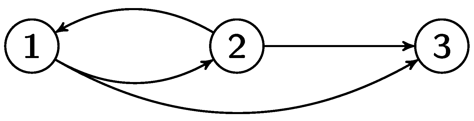
In this section, we illustrate in a specific example how the expected (discounted) cumulative payment $\mathbb{E}[{\widehat{D}}_T]$ from Lemma 3 can be calculated by using the explicit expression of the components $F^i(t,T)$ from the previous section and the connection established through Equation (9). In the following, we regard a specific insurance product, namely an income protection insurance, and for simplicity we assume that the corresponding process X of the insured person can only take the three states $\mathcal{K}=\{1=healthy,2=\mathit{\text{sick/unfit}}\mathit{\text{for}}\mathit{\text{work}},3=death\}$, where state 3 is absorbing. The corresponding transitions are illustrated in Figure 1.

Hence, for ${\mathbf{b}}^{j,k}\in {\mathbb{R}}^3$, $c^{j,k}\in \mathbb{R}$ from Equation (19) we set ${\mathbf{b}}^{j,k}=\mathbf{0}$ and $c^{j,k}=0$ for $(j,k)\notin \mathcal{I}:=\left\{\right(1,2),(2,1),(1,3),(2,3\left)\right\}$.

In the following, we assume a specific form for the Markov process μ from Equation (19), namely a simple, 3-dimensional Ornstein-Uhlenbeck (OU) process with corresponding SDE

$$d{\mathit{\mu }}_t=\mathbf{a}{\mathit{\mu }}_{t}dt+\mathit{\sigma }d{\mathbf{W}}_t,{\mathit{\mu }}_0=\mathit{\xi }\in {\mathbb{R}}^3$$

Note that for the OU process it is well-known that Condition (23) for the expectation is fulfilled. A major drawback, though, of choosing this process for the intensity is the undesirable feature that it can become negative with positive probability. However, [31] provide calibrated parameters for which the probability of negative values for μ turns out to be negligible. For this reason, we choose similar parameter values and set

$$\mathbf{a}={(0.07,0.11,0.09)}^{⊺},\mathit{\sigma }=\left(\begin{array}{ccc}0.0003& 0& 0\\ 0& 0.0007& 0\\ 0& 0& 0.0005\end{array}\right)\text{and}\mathit{\xi }={(0.1,0.1,0.1)}^{⊺}$$

Hence, Equations (21) and (22) simplify and yield to

$$\begin{array}{cc}& \mathit{\delta }(t,\mathbf{x})={\left({\mathbf{d}}^1\right)}^{⊺}\mathbf{x}\hfill \\ & {\left[\mathit{\sigma }(t,\mathbf{x})\mathit{\sigma }{(t,\mathbf{x})}^{⊺}\right]}_{i,j}={\left[{\mathbf{V}}^0\right]}_{i,j}\hfill \end{array}$$

with

$${\mathbf{d}}^1=\left(\begin{array}{ccc}{a}_1& 0& 0\\ 0& a_2& 0\\ 0& 0& a_3\end{array}\right)\text{and}{\mathbf{V}}^0=\left(\begin{array}{ccc}{\mathit{\sigma }}_{11}^2& 0& 0\\ 0& {\mathit{\sigma }}_{22}^2& 0\\ 0& 0& {\mathit{\sigma }}_{33}^2\end{array}\right)$$

As a consequence of these assumptions, the ODEs Equations (29)–(36) substantially simplify and can be explicitly solved, see e.g., [32]. For example, for every $0\le t\le u\le T$ and every choice of $(i,j)\in \mathcal{I}$, the ODEs Equations (29) and (30) now are given by

$$\begin{array}{cc}& \frac{d{\mathit{\beta }}_u^{i,j}}{dt}\left(t\right)={\mathbf{b}}^{i,j}-{\mathbf{d}}^1{\mathit{\beta }}_u^{i,j}\left(t\right)\hfill \\ & \frac{d{\alpha }_u^{i,j}}{dt}\left(t\right)=c^{i,j}-\frac{1}{2}{\left({\mathit{\beta }}_u^{i,j}\left(t\right)\right)}^{⊺}{\mathbf{V}}^0{\mathit{\beta }}_u^{i,j}\left(t\right)\hfill \end{array}$$

with terminal conditions ${\alpha }_u^{i,j}\left(u\right)=0$ and ${\mathit{\beta }}_u^{i,j}\left(u\right)=0$. For the k-th components of ${\mathit{\beta }}_u^{i,j}\left(t\right)$, i.e., ${}^{\left(k\right)}{\beta }_u^{i,j}\left(t\right)$, one obtains the explicit solutions

$${}^{\left(k\right)}{\beta }_u^{i,j}\left(t\right)=\frac{b_k^{i,j}}{d_{kk}^1}(1-exp(d_{kk}^1(u-t)),k\in \{1,2,3\}$$

and

$$\begin{array}{cc}\hfill {\alpha }_u^{i,j}\left(t\right)=& -c^{i,j}(u-t)+\frac{1}{2}\sum _{k=1}^3\frac{{\sigma }_k^2{\left(b_k^{i,j}\right)}^2}{{\left(d_{kk}^1\right)}^2}\left[(u-t)-\frac{2}{d_{kk}^1}(1-exp(d_{kk}^1(u-t))\right.\hfill \\ & \left.+\frac{1}{2d_{kk}^1}(1-exp(2d_{kk}^1(u-t))\right]\hfill \end{array}$$

Similarly, the ODEs of the remaining Equations (31)–(36) can be derived.

Next, we need to specify all remaining parameters, i.e., ${\mathbf{b}}^{j,k},c^{j,k}$ for $(j,k)\in \mathcal{I}$, the components $\mathbf{A},$ $\mathbf{Y},\mathbf{Z}$ of the quadruple $(X;\mathbf{A};\mathbf{Y};\mathbf{Z})$ and the discounting factor $S_0$. For simplicity, we set $S_0=e^{-rt}$ with a constant interest rate r and choose

$${\mathbf{b}}^{1,2}={\mathbf{b}}^{2,1}=\left(\begin{array}{c}3\\ 3\\ 3\end{array}\right),{\mathbf{b}}^{1,3}=\left(\begin{array}{c}1\\ 1\\ 1\end{array}\right),{\mathbf{b}}^{2,3}=\left(\begin{array}{c}2\\ 2\\ 2\end{array}\right),c^{1,2}=c^{2,1}=1,c^{1,3}=0.1,c^{2,3}=0.2$$

We have chosen the components of ${\mathbf{b}}^{j,k}$ to be equal in order to emphasize the general dependence of the process ${\psi }_t^{j,k}$ in Equation (19) on ${\mathit{\mu }}_t$ and not on the specific linear combination.

Furthermore, similar to Example 2, we set

$$\mathbf{Z}:=\left(\begin{array}{ccc}0& 0& z\\ 0& 0& z\\ 0& 0& 0\end{array}\right),\mathbf{Y}\equiv 0,\text{and}{\mathbf{A}}_t={\mathbf{C}}_t-{\mathbf{P}}_t,t\in [0,T]$$

with ${\mathbf{C}}_t$ and ${\mathbf{P}}_t$ representing the cumulative state-dependent claim payments (e.g., annuities) and insurance premiums up to maturity, respectively, and z the “immediate” claim payment if the insured person dies. More precisely, we assume monthly equal insurance premiums and claim payments equal to 1, if the insured person is in the states 1 (healthy) or 2 (sick/unfit for work), respectively, and which are paid at the end of each month in a proportional way. Let the payment dates $0<T_1<T_2<\dots$ denote the final day of each month, i.e., $T_i=\frac{i}{12}$, then we set

$$\mathit{\nu }\left(t\right)=\left(\begin{array}{c}1/\Delta t\\ -1/\Delta t\\ 0\end{array}\right)$$

with $\Delta t=1/12$ and ${\mathbf{A}}_t={\int }_0^t\mathit{\nu }\left(s\right)ds$.

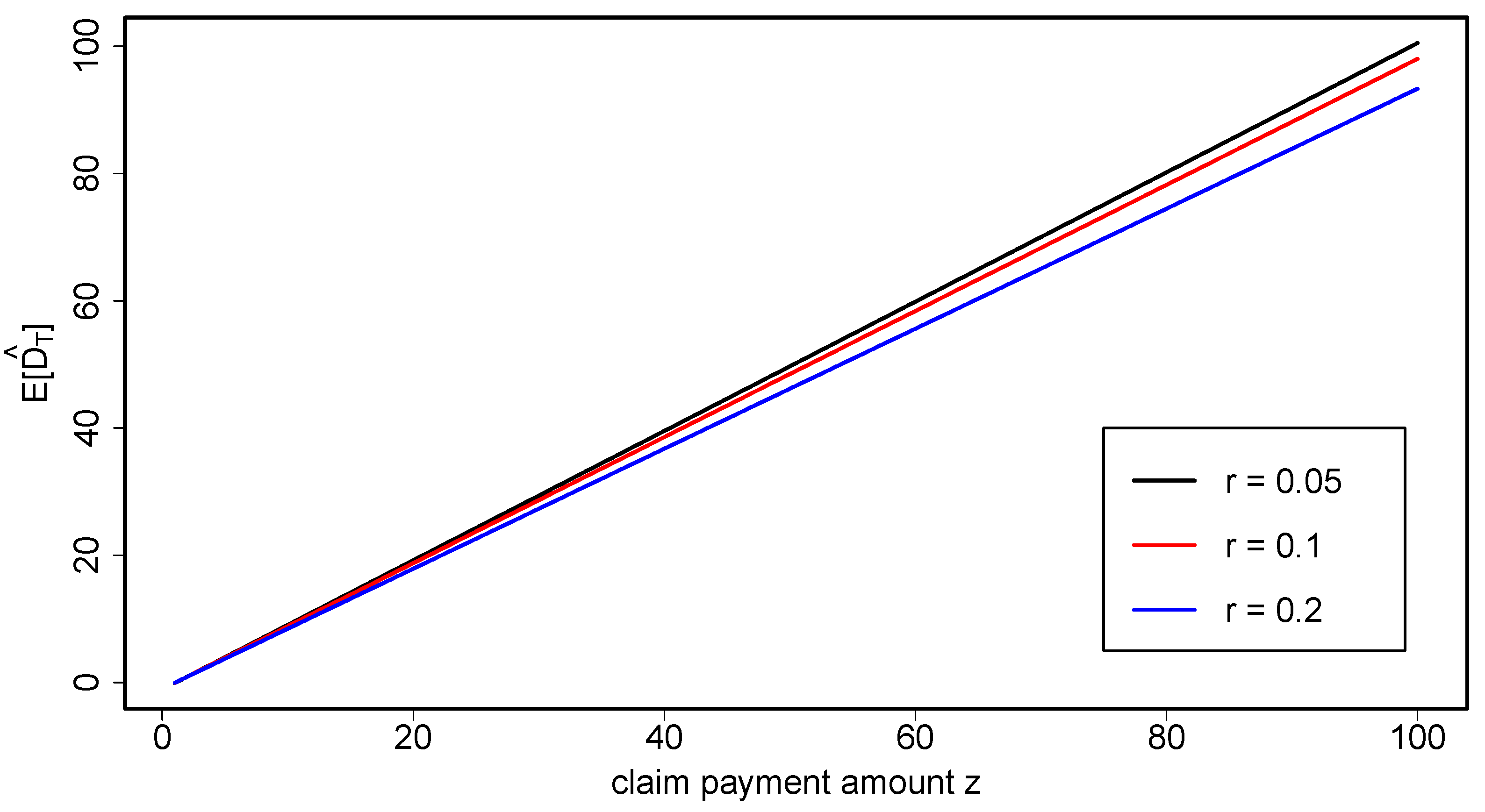
Clearly, with these specifications Assumption 6 is fulfilled. Finally, assuming that the insured persons process X starts in the state 1 (healthy) at $t=0$, one obtains ${\mathbf{H}}_0^{⊺}=(1,0,0)$. Based on the explicit result for $F^i(0,T)$ from Equation (41), now we are able to calculate the expected (discounted) cumulative payment $\mathbb{E}[{\widehat{D}}_T]$ from Lemma 3 in $t=0$, depending on the claim payment amount z, which is payed when the insured person dies, and on the constant interest rate r. The corresponding integrals involved in Equation (41) are approximated using the integrate function in the statistical software program R ([33]).

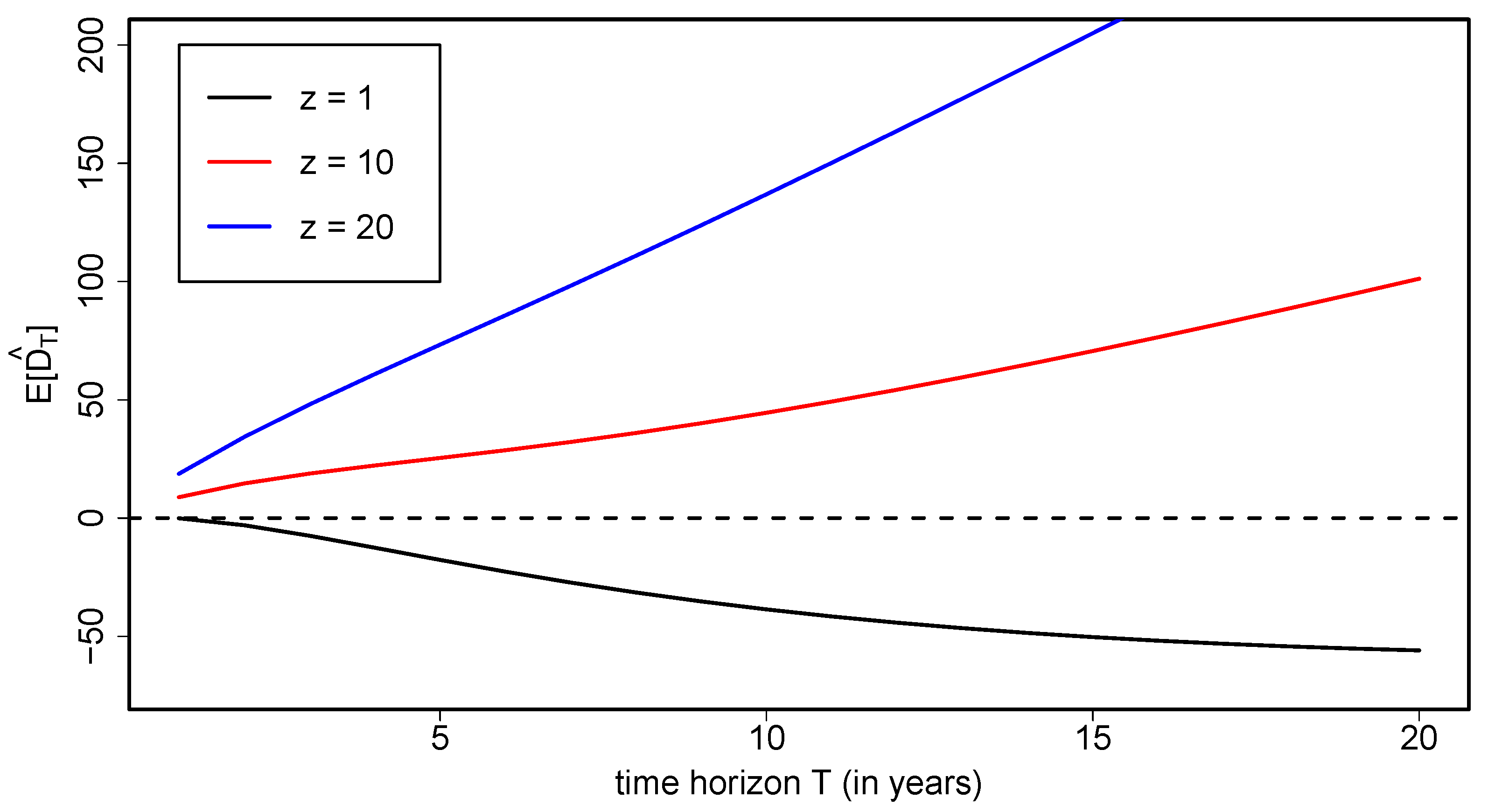
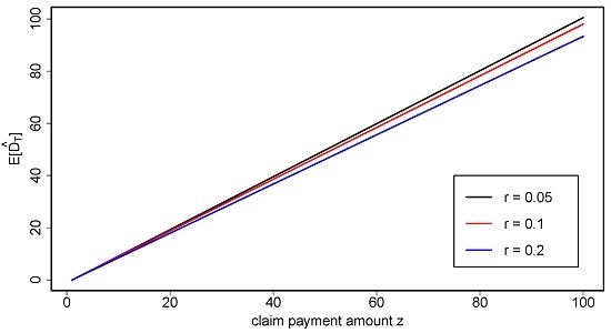
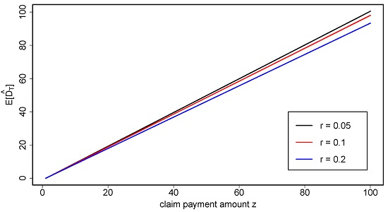
Figure 2 illustrates the expected cumulative payment $\mathbb{E}[{\widehat{D}}_T]$ as a function of the claim payment amount z, a time horizon of one year ($T=1$) and three different values of the constant interest rate r. In Figure 3, the expected cumulative payment $\mathbb{E}[{\widehat{D}}_T]$ are displayed against the time horizon T, for three different values of the claim payment amount z and for a constant interest rate $r=0.1$.

4. Conclusions

In this paper, we consider pricing and hedging of general insurance contracts by means of risk minimization. We model the individual progress in time of visiting an insurance policy’s states by using $\mathbb{F}$-doubly stochastic Markov chains. In this way we are able to consider a multi-state setting to describe different types of insurance benefits and to include the influence of market conditions and external risk factors on the evolution of the insured person among the policy’s states as well as on the insurance benefits, when they are linked to some financial performance. We explicitly provide the risk-minimizing strategy for an insurance contract in a Brownian financial market setting and specify it within an affine structure for the intensity. The results are illustrated by a numerical example, which shows how this technical setting can actually be easily implemented.

References

F. Biagini, and I. Schreiber. “Risk minimization for life insurance liabilities.” SIAM J. Financ. Math. 4 (2013): 243–264. [Google Scholar] [CrossRef]
F. Biagini, T. Rheinländer, and J. Widenmann. “Hedging mortality claims with longevity bonds.” ASTIN Bull. 43 (2013): 123–157. [Google Scholar] [CrossRef]
D. Blake, A.J.G. Cairns, and K. Dowd. “The birth of the life market.” Asia-Pac. J. Risk Insur. 3 (2008): 6–36. [Google Scholar] [CrossRef]
H. Föllmer, and D. Sondermann. “Hedging of non-redundant contingent claims.” In Contributions to Mathematical Economics. Edited by A. Mas-Colell and W. Hildenbrand. Haarlem, The Netherlands: North Holland, 1986, pp. 205–223. [Google Scholar]
T. Møller. “Risk-Minimizing Hedging Strategies for Insurance Payment Processes.” Finance Stoch. 5 (2001): 419–446. [Google Scholar] [CrossRef]
J.P. Ansel, and C. Stricker. “Décomposition de Kunita-Watanabe.” In Séminaire de Probabilités XXVII. Lecture Notes in Mathematics Volume 1557; Berlin, Germany: Springer, 1993. [Google Scholar]
H. Kunita, and S. Watanabe. “On square integrable martingales.” Nagoya Math. J. 30 (1967): 209–245. [Google Scholar]
J. Hoem. “Markov Chain Models in Life Insurance.” In Blätter der Deutschen Gesellschaft für Versicherungs- und Finanzmathematik. Berlin, Germany: Springer, 1969, Volume 9, pp. 91–107. [Google Scholar]
R. Norberg. “Hattendorff’s theorem and Thiele’s differential equation generalized.” Scand. Actuar. J. 1 (1992): 2–14. [Google Scholar] [CrossRef]
R. Norberg. “A Theory of Bonus in Life Insurance.” Finance Stoch. 3 (1999): 373–390. [Google Scholar] [CrossRef]
R. Norberg. “Optimal hedging of demographic risk in life insurance.” Finance Stoch. 17 (2013): 197–222. [Google Scholar] [CrossRef]
J. Jakubowski, and M. Niewęgłowski. “A class of F-doubly stochastic Markov chains.” Electron. J. Probab. 15 (2010): 1743–1771. [Google Scholar] [CrossRef]
F. Biagini, A. Groll, and J. Widenmann. “Intensity-based premium evaluation for unemployment insurance products.” Insur.: Math. Econ. 53 (2013): 302–316. [Google Scholar] [CrossRef]
J. Barbarin. “Heath-Jarrow-Morton modelling of longevity bonds and the risk minimization of life insurance portfolios.” Insur.: Math. Econ. 43 (2008): 41–55. [Google Scholar] [CrossRef]
F. Biagini, and A. Cretarola. “Quadratic Hedging Methods for Defaultable Claims.” Appl. Math. Optim. 56 (2007): 425–443. [Google Scholar] [CrossRef]
F. Biagini, and A. Cretarola. “Local Risk-Minimization for Defaultable Markets.” Math. Financ. 19 (2009): 669–689. [Google Scholar] [CrossRef]
F. Biagini, and A. Cretarola. “Local Risk-Minimization for defaultable claims with recovery process.” Appl. Math. Optim. 65 (2012): 293–314. [Google Scholar] [CrossRef]
F. Biagini, T. Rheinländer, and I. Schreiber. “Risk-minimization for life insurance liabilities with basis risk.” Math. Financ. Econ. 10 (2016): 151–178. [Google Scholar] [CrossRef]
F. Biagini, C. Botero, and I. Schreiber. “Risk-minimization for life insurance liabilities with dependent mortality risk.” Math. Finance, 2015. [Google Scholar] [CrossRef]
T.R. Bielecki, M. Jeanblanc, and M. Rutkowski. “Pricing and trading credit default swaps in a hazard process model.” Ann. Appl. Probab. 18 (2008): 2495–2529. [Google Scholar] [CrossRef]
J. Jakubowski, and M. Niewęgłowski. “Pricing and Hedging of Rating-Sensitive Claims Modeled by -doubly stochastic Markov chains.” In Advanced Mathematical Methods for Finance. Edited by G. DiNunno and B.O. Ksendal. Berlin, Germany: Springer, 2011, pp. 417–454. [Google Scholar]
F. Biagini, A. Cretarola, and E. Platen. “Local risk-minimization under the benchmark approach.” Math. Financ. Econ. 8 (2014): 109–134. [Google Scholar] [CrossRef]
F. Biagini. “Evaluating hybrid products: The interplay between financial and insurance markets.” In Seminar on Stochastic Analysis, Random Fields and Applications VII, Centro Stefano Franscini, Ascona, May 2011. Edited by R. Dalang, M. Dozzi and F. Russo. Basel, Switzerland: Springer & Birkhäuser, 2013, pp. 285–304. [Google Scholar]
J. Widenmann. “Pricing and Hedging Insurance Contracts in Hybrid Markets.” Ph.D. Thesis, Ludwig Maximilians University Munich, Munich, Germany, 2013. [Google Scholar]
E. Platen, and D. Heath. A Benchmark Approach to Quantitative Finance. Berlin, Germany: Springer, 2007. [Google Scholar]
M. Schweizer. “A guided tour through quadratic hedging approaches.” In Option Pricing, Interest Rates and Risk Management. Edited by E. Jouini, J. Cvitanic and M. Musiela. Cambridge, UK: Cambridge University Press, 2001, pp. 538–574. [Google Scholar]
L.F.B. Henriksen, and T. Møller. “Local risk-minimization with survivor bonds.” Appl. Stoch. Models Bus. Ind. 31 (2015): 241–263. [Google Scholar] [CrossRef]
P.E. Protter. Stochastic Integration and Differential Equations, 2nd ed. New York, NY, USA: Springer, 2005. [Google Scholar]
E. Biffis. “Affine processes for dynamic mortality and actuarial valuation.” Insur.: Math. Econ. 37 (2005): 443–468. [Google Scholar] [CrossRef]
D. Duffie, J. Pan, and K. Singleton. “Transform analysis and asset pricing for affine jump-diffusions.” Econometrica 68 (2000): 1343–1376. [Google Scholar] [CrossRef]
E. Luciano, and E. Vigna. “Mortality Risk via affine stochastic intensities: Calibration and empirical relevance.” Belg. Actuar. Bull. 8 (2008): 5–16. [Google Scholar]
D. Filipović. Term-Structure Models. Berlin, Germany: Springer, 2009. [Google Scholar]
R.C. Team. R: A Language and Environment for Statistical Computing. Vienna, Austria: R Foundation for Statistical Computing, 2015. [Google Scholar]
D. Lando. “On Cox processes and credit risk securities.” Rev. Deriv. Res. 2 (1998): 99–120. [Google Scholar] [CrossRef]
T. Bielecki, and M. Rutkowski. Credit Risk: Modelling, Valuation and Hedging, 2nd ed. Berlin, Germany: Springer-Finance, Springer, 2004. [Google Scholar]
M. Schweizer. “Local Risk-Minimization for Multidimensional Assets and Payment Streams.” Warszawa, Poland: Banach Center Publications, 2008, Volume 83, pp. 213–229. [Google Scholar]
J. Barbarin. “Valuation, Hedging and the Risk Management of Insurance Contracts.” Ph.D. Thesis, Université Catholique de Louvain, Louvain, Belgium, 2008. [Google Scholar]
Figure 1.
Possible transitions for an insured person’s process in an income protection insurance with the three states with absorbing state 3.
Figure 2.
Expected (discounted) cumulative payments as a function of the claim payment amount z and for three different constant interest rate values r for a time horizon of one year, i.e., .
Figure 3.
Expected (discounted) cumulative payments as a function of the time horizon T (in years) and three different claim payment amounts z and for a constant interest rate .
Biagini, F.; Groll, A.; Widenmann, J.