1. Introduction
Traditional participating (i.e., non-linked) life insurance products have come under significant pressure in the current environment with low interest rates and capital requirements based on risk-based solvency frameworks such as Solvency II or the Swiss Solvency Test (SST). This is due to the fact that these products usually come with very long-term and year-by-year (cliquet-style) guarantees which make them rather risky (and hence capital intensive) from an insurer’s perspective. For this reason, participating products that come with alternative forms of guarantees have been developed in several countries and are currently discussed intensively.
Different aspects like the financial risk and the fair valuation of interest rate guarantees in participating life insurance products have been analyzed, e.g., in Briys and de Varenne [
1], Grosen and Jørgensen [
2], Grosen
et al. [
3], Grosen and Jørgensen [
4], Mitersen and Persson [
5], Bauer
et al. [
6], Kling
et al. [
7], Kling
et al. [
8], Barbarin and Devolder [
9], Gatzert and Kling [
10], Gatzert [
11] and Graf
et al. [
12]. For more details on this literature, see e.g., the literature overview in Reuß
et al. [
13].
Some authors analyze participating life insurance contracts also from a policyholder’s perspective. Bohnert and Gatzert [
14] examine the impact of three typical surplus distribution schemes on the insurer’s shortfall risk and the policyholder’s net present value. They conclude that, even though the amount of surplus is always calculated the same way, the surplus distribution scheme has a substantial impact. Gatzert
et al. [
15] compare the different perspectives of policyholders and insurers concerning the value of a contract. They identify contracts that maximize customer value under certain risk preferences while keeping the contract value for the insurer fixed.
Finally, Reuß
et al. [
13] introduce participating products with alternative forms of guarantees. They analyze the impact of alternative guarantees on the capital requirement under risk-based solvency frameworks and introduce the concept of Capital Efficiency which relates profits to capital requirements.
Introducing such alternative guarantees primarily attempts to reduce the insurer’s risk. Typically, this would
ceteris paribus make such contracts less attractive from a policyholder’s perspective. Since in the current market environment some insurers find it rather difficult to continue offering contracts with guarantees at all (and some have already stopped new business in participating contracts or switched to products with a lower protection level),
1 products with somewhat weaker forms of guarantees might be a way to at least continue offering some products that are attractive to risk-averse policyholders seeking guarantees. In this paper, we therefore analyze how participating products can be modified in terms of surplus participation and asset allocation with the objective of balancing the interests of policyholders and the insurer. We particularly take into account that policyholders may demand some kind of “compensation” for the modified guarantees since these may lead to lower benefits than the traditional product in certain adverse scenarios.
The remainder of this paper provides a possible approach for this objective. In
Section 2, we present the three considered contract designs from Reuß
et al. [
13] that all come with the same level of guaranteed maturity benefit but with different types of guarantee. As a reference, we consider a traditional contract with a cliquet-style guarantee based on a guaranteed interest rate >0%. The first alternative product has the same guaranteed maturity benefit which is, however, valid only at maturity; additionally, there is a 0% year-to-year guarantee on the account value, meaning that the account value cannot decrease from one year to the next. The second alternative product finally only has the (same) guaranteed maturity benefit. But in this product there is no year-to-year guarantee on the account value at all, meaning that the account value may decrease in some years. On top of the different types of guarantees, all three products include a surplus participation depending on the insurer’s realized investment return.
In
Section 3, we introduce our stochastic model for the stock market return and the short-rate process. We then describe how the evolution of the insurance portfolio and the insurer’s balance sheet are projected in our asset-liability model. The considered asset allocation consists of bonds with different maturities and an equity investment. The model also incorporates management rules as well as typical intertemporal risk-sharing mechanisms (e.g., building and dissolving unrealized gains and losses), which are an integral part of participating contracts in many countries and should therefore not be neglected.
In
Section 4, we present the results of our analyses. First, for all considered product types, we determine combinations of asset allocation and surplus participation rate that all come with the same expected profit from the insurer’s perspective (“iso-profit” products). Hence, from a policyholder’s view, the risk-neutral values of all these contracts are also identical,
i.e., all these products would be considered equally fair in a fair value framework. Then, we have a closer look at those iso-profit product designs with alternative guarantees that come with the same asset allocation as the traditional product.
2 We find that for the alternative products, the insurer’s risk measured by the Solvency II capital requirement is significantly reduced. Unfortunately, they might appear less attractive from the policyholder’s perspective. Therefore, we also consider iso-profit products with alternative guarantees that come with a higher equity ratio. For this set of product designs, the insurer’s risk can lie anywhere between the reduced risk and the risk of the traditional product.
3 We then analyze the real-world risk-return distribution of products from the policyholder’s perspective and find that products can be designed which only slightly increase the policyholder’s risk (although they significantly reduce the insurer’s capital requirement) and significantly increase the policyholder’s real-world expected return (although the insurer’s risk-neutral expected profit remains unchanged). We therefore conclude that carefully designed participating products with modified guarantees might be suitable for reconciling the insurer’s and policyholders’ interests.
Section 5 concludes and provides an outlook on further research.
2. Considered Products
The three product designs that will be analyzed are the same as in Reuß
et al. [
13]. We therefore only briefly describe the most important product features and refer to that paper for more details.
All three considered products provide a guaranteed benefit at maturity based on regular (annual) premium payments . The prospective actuarial reserves for the guaranteed benefit that the insurer has to set up at time t is given by . Furthermore, denotes the client’s account value at time consisting of the sum of the actuarial reserve and any surplus (explained below) that has already been credited to the policyholder. At maturity, is paid out as maturity benefit.
We do not assume one single “technical interest rate”, but rather define three different interest rates: a pricing interest rate
that determines the ratio between the annual premium
and the guaranteed maturity benefit
, a reserving interest rate
, that is used for the calculation of the actuarial reserve
, and a year-to-year guaranteed interest rate
, which corresponds to the minimum return that the client has to receive each year on the account value
.
4With annual charges
, the actuarial principle of equivalence
5 yields
Based on the reserving rate
, the actuarial reserve
at time
t is given by
As in Reuß
et al. [
13], we assume that in case of death or surrender in year
, the current account value
is paid at the end of year
.
6 Therefore, mortality rates are not relevant in the formulae above.
Annual surplus is typically credited to such policies according to country-specific regulation. In Germany, at least of the (local GAAP book value) investment income on the insurer’s assets (but not less than defined below) has to be credited to the policyholders’ accounts.
In previous years, in many countries so-called cliquet-style guarantees prevailed, where all three interest rates introduced above coincide and this single rate is referred to as guaranteed rate or technical rate. In such products, typically, any surplus credited to the contract leads to an increase of the guaranteed maturity benefit and this increase is also calculated based on the same technical rate. Our more general setting includes this product as the special case .
Note that the regulatory requirements regarding reserving and minimum surplus participation limit the potential for diversification over time.
7The “required yield” on the account value in year
t is given by
This definition makes sure that the account value remains non-negative, never falls below the actuarial reserve, and earns at least the year-by-year guaranteed interest rate. With
denoting the annual surplus, the account value evolves according to
If the pricing rate exceeds the year-by-year guaranteed interest rate, the required yield decreases if surplus (which is included in ) has been credited in previous years. Hence, for such products (contrary to the traditional product), distributing surplus to the client decreases the insurer’s risk in future years.
We consider three concrete product designs that all come with the same level of the maturity guarantee (based on a pricing rate of 1.75%) but with a different type of guarantee.
8- -
Traditional, cliquet-style product:
- -
Alternative 1 product with a 0% year-by-year guarantee: ,
- -
Alternative 2 product without any year-by-year guarantee: ,
Although all three products come with the same guaranteed maturity benefit, they come with a different risk for the policyholder in the sense that for the alternative products it is more likely that the actual maturity benefit will be at or close to the guaranteed value. To illustrate this, consider the simplified example of a contract with two years term to maturity and a maturity guarantee based on an interest rate of 1.75%. Now, assume that the asset return to be credited to the policyholder’s account (i.e., of the book value return as described above) would be 6% in year one and 0% in year two. In the traditional design, the policyholder would receive 6% in year one and still the year-by-year guaranteed rate of 1.75% in year two. In the alternative designs, the policyholder would receive 6% in year one. The required yield would then drop to zero and the policyholder would receive 0% in year two.
In our numerical analyses, we assume that all policyholders are 40 years old at inception of the respective contract, that the considered pool of policies decreases due to mortality, which is based on the German standard mortality table (DAV 2008 T), and that no surrender occurs. Furthermore, we assume annual administration charges
throughout the contract’s lifetime, and acquisition charges
which are equally distributed over the first five years of the contract. Hence,
. Furthermore, we assume that expenses coincide with the charges. The product parameters are given in
Table 1.
3. Stochastic Modeling and Assumptions
The framework for the financial market model and for the projection of the insurer’s balance sheet and cash flows, including management rules and surplus distribution (which is based on local GAAP book values), is taken from Reuß
et al. [
13]. We therefore keep the following subsections brief and refer to that paper for more details.
3.1. The Financial Market Model
We assume that assets are invested in coupon bonds and equity. Cash flows arising between annual re-allocation dates are invested in a riskless bank account. Since we will perform analyses in both a risk-neutral and a real-world framework, we specify dynamics under both measures. We let the short rate process
follow a Vasicek
9 model, and the equity index
follow a geometric Brownian motion and get the following risk-neutral dynamics:
where
and
are independent Wiener processes on some probability space
with a risk-neutral measure
and the natural filtration
. Assuming a constant market price of interest rate risk
, the corresponding real-world dynamics are given by:
where
,
includes an equity risk premium and
,
are independent Wiener processes under a real-world measure
.
The parameters
,
and
are deterministic and constant. For the purpose of performing Monte Carlo simulations, the above equations can be solved to
in the risk-neutral case. It can be shown that the four integrals in the formulae above follow a joint normal distribution.
10 Monte Carlo paths are calculated using random realizations of this multidimensional distribution. Similarly, we obtain
for the real-world approach. In both settings, the initial value of the equity index
and the initial short rate
are deterministic parameters.
The bank account is given by
and the discretely compounded yield curve at time
by
11
for any time
and term
. Based on the yield curve, we can calculate the par-yield that determines the coupon rate of the considered coupon bond.
In our numerical analyses, we use market parameters shown in
Table 2. The parameters
,
,
and
are directly adopted from Graf
et al. [
12]. The choice of the parameters
,
and
reflects lower interest rate and equity risk premium levels.
3.2. The Asset-Liability Model
The insurer’s simplified balance sheet at time
is given by
Table 3 (the rather simple structure is justified in Reuß
et al. [
13]).
The liability side of the balance sheet consists of the account value
(defined in
Section 2) and the shareholders’ profit or loss
in year
t.
12On the asset side, we have the book value of bonds , which coincides with the nominal amount under German GAAP since we assume that bonds are considered as held to maturity. For the book value of the equity investment the insurer has more discretion. We assume that the insurer wants to create rather stable book value returns (and hence surplus distributions) in order to signal stability to the market. Therefore, a ratio of the unrealized gains or losses (UGL) of equity is realized annually if (i.e., in case of unrealized gains) and a ratio of the UGL is realized annually if . In particular, has to be chosen in a legal framework, where unrealized losses on equity investments are not possible.
At the end of the year, the following rebalancing is implemented: market values of all assets (including the bank account) are derived and a constant ratio is invested in equity. The remainder is invested in bonds.
For new bond investments, coupon bonds yielding at par with a given term are used until all insurance contracts’ remaining terms are less than years. Then, we invest in bonds with a term that coincides with the longest remaining insurance contracts. If bonds need to be sold, they are sold proportionally to the market values of the different bonds in the existing portfolio.
Finally, the book value return on assets is calculated for each year in each simulation path as the sum of coupon payments from bonds, interest payments on the bank account, and the realization of UGL. The split between policyholders and shareholders is driven by the participation rate
introduced in
Section 2. If the policyholders’ share is not sufficient to pay the required yields to all policyholders, there is then no surplus for the policyholders, and all policies receive exactly the respective required yield
. Otherwise, surplus is credited which amounts to the difference between the policyholders’ share of the asset return and the cumulative required yield. Following the typical practice, as, e.g., in Germany, we assume that this surplus is distributed among the policyholders such that all policyholders receive the same client’s yield (defined by the required yield plus surplus rate), if possible.
13The insurer’s profit/loss
results as the difference between the total investment income and the amount credited to all policyholder accounts. We assume that
leads to a corresponding cash flow to or from the shareholders at the beginning of the next year; that means, particularly, that a loss is compensated by the insurer’s shareholders.
14In our numerical analyses we let years, , and
3.3. The Projection Setup
We use a deterministic projection for the past (
i.e., until
) to build up a portfolio of policies for the analysis. This portfolio consists of 1000 policies that had been sold each year in the past 20 years. Hence, at
, we have a portfolio with remaining times to maturity between one year and 19 years.
15 Therefore the time horizon for the stochastic projection starting at
amounts to
years. In the deterministic projection before
, we use a flat yield curve of 3.0% (consistent with the mean reversion parameter
of the stochastic model after
), and management rules described above.
Then, starting at , stochastic projections are performed for this portfolio. In line with the valuation approach under Solvency II and MCEV, we do not consider new business after for the calculation of the insurer’s profitability and risk. We do, however, consider new business when calculating the risk-return characteristics from the policyholder’s perspective.
We assume that the book value of the asset portfolio at coincides with the book value of liabilities. The initial amount of UGL is derived from a base case projection of the traditional product with an equity ratio of and a participation rate of . This value is used as the initial UGL (before solvency stresses or sensitivities) for the projections of all products. The coupon bond portfolio at consists of bonds with a uniform coupon of 3.0%, where the time to maturity is equally split between one year and years.
For all projections, the number of scenarios is
. Further analyses showed that this allows for stable results.
16 4. Results
In Reuß
et al. [
13], it was shown that a modification of the products reduces the insurer’s risk and increases the insurer’s profitability. Obviously, such products are less attractive for the policyholder since they pay lower benefits at least in some possible scenarios. Therefore, it is currently intensively discussed among practitioners how policyholders can be compensated for this fact and whether the resulting products are then still attractive for the insurer.
17 In this section, we show how products can be designed that “give back” some or all of the increased profitability and the reduced risk to the policyholder.
4.1. Analysis of the Insurer’s Profit
In a first step, we consider alternative products that achieve the same profitability (“iso-profit”) as the traditional product by using suitable combinations of the equity ratio and the profit participation rate .
To measure the insurer’s profitability in a market-consistent framework we use the expected present value of future profits (PVFP) under the risk-neutral measure
.
18The Monte Carlo estimate for the PVFP is calculated by
where
is the number of scenarios,
denotes the insurer’s profit/loss in year
in scenario
,
is the value of the bank account after
years in scenario
, and hence
is the present value of future profits in scenario
.
The PVFP for the traditional product in our base case scenario is given by 3.62% (as a percentage of the present value of future premium income) using
(which is the minimum profit participation rate required under German regulation) and an equity ratio of
.
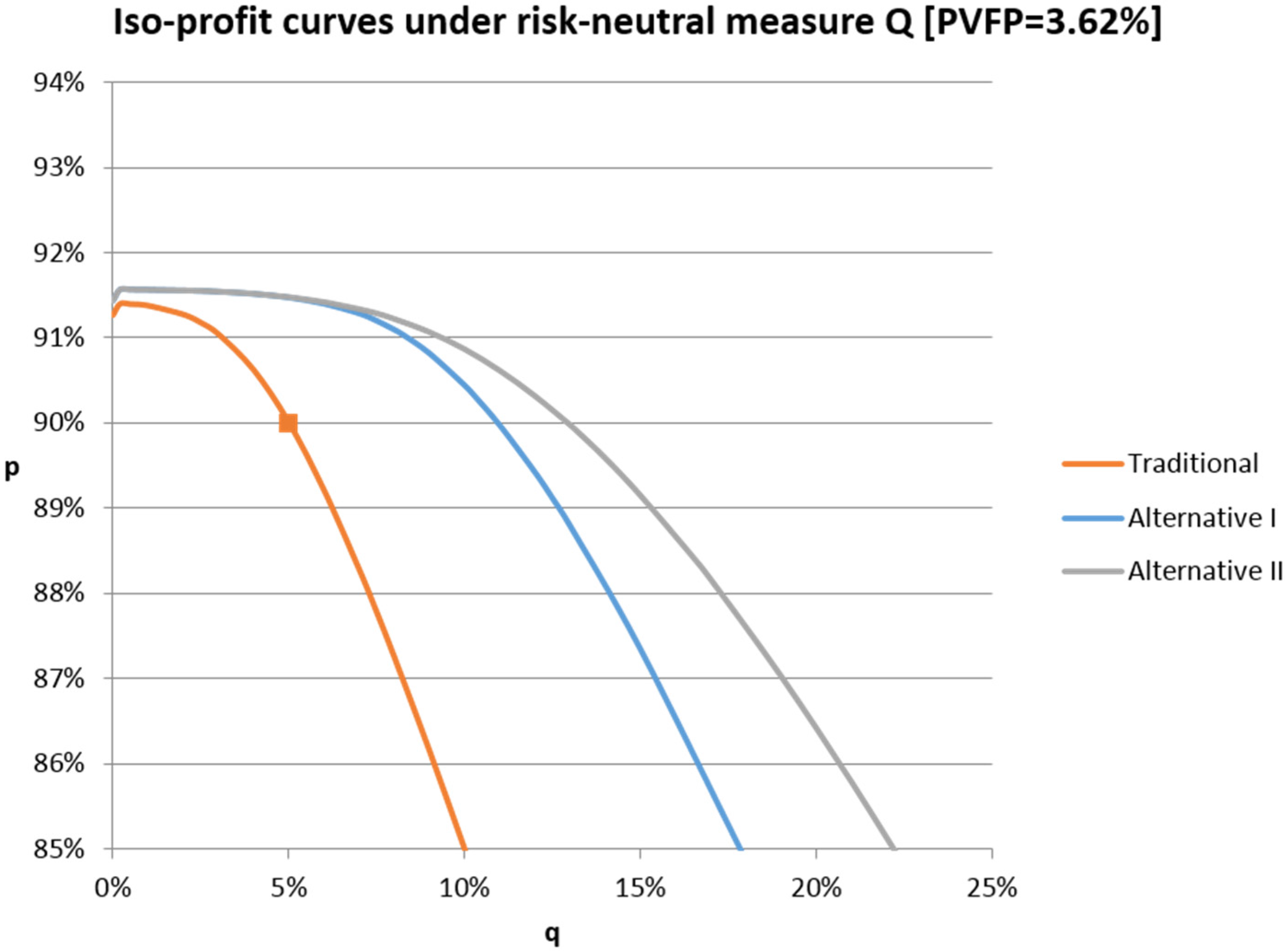
Figure 1 shows combinations of
and
that lead to the same PVFP for all three considered products.
Obviously, for all products, the insurer’s risk resulting from an increased equity ratio has to be compensated by a reduced participation rate in order to keep the PVFP unchanged. Only for very low equity ratios (below 0.5%), we observe the opposite effect. This is caused by the missing diversification effects between bonds and stocks which leads to an increase in risk if the equity ratio is further reduced.
We find that for a given participation rate, the alternative products allow for a significantly higher equity ratio if the insurer wants to keep the PVFP unchanged. As expected, the effect is stronger for the Alternative 2 product. Note that the difference between Alternative 1 and 2 is negligible for equity ratios below 7% since for low equity ratios the probability for a year with negative client’s yield in the Alternative 2 product (which is the only situation where the two alternative products differ) is very low.
If the insurer intends to keep the participation rate at the legally required minimum of 90%, the equity ratio could be increased from 5% to roughly
19 10.75% for the Alternative 1 product and to 12.75% for the Alternative 2 product. This would increase the policyholder’s expected return without affecting the insurer’s expected profit.
Conversely, if the equity ratio remains unchanged at 5%, the participation rate could be increased to 91.48%, with unchanged PVFP.
Note that, in our setting, products with identical PVFP from the insurer’s perspective automatically have the same fair value (in a risk-neutral framework) from the policyholder’s perspective. Therefore, if a fair value approach is taken to analyze products from the policyholder’s perspective, all “iso-profit” products are equally fair. However, following, e.g., Graf
et al. [
29], we will also analyze the products’ risk-return characteristics in a real-world framework in
Section 4.3.
4.2. Analysis of the Insurer’s Risk
Of course, the products from the previous subsection, which all come with the same expected profit from the insurer’s perspective, differ in terms of risk for the insurer. Therefore, we now analyze the insurer‘s risk resulting from these “iso-profit” products. We use the insurer‘s Solvency Capital Requirement for market risk (
) as a measure for risk and consider only interest rate and equity risk as part of the market risk
20. To determine
, we calculate the PVFP under an interest rate stress of 100 bps
,
i.e., using
and
. Furthermore, we calculate the PVFP under a stress of the initial market value of equities (
), using a reduction of 39% according to the Solvency II standard formula
21. Then, the Solvency Capital Requirement for interest rate risk is determined by
and the Solvency Capital Requirement for equity risk is determined by
. According to the standard formula of the Solvency II framework, the aggregated SCR for market risk is then calculated by
with a correlation of
between the interest rate and equity risk.
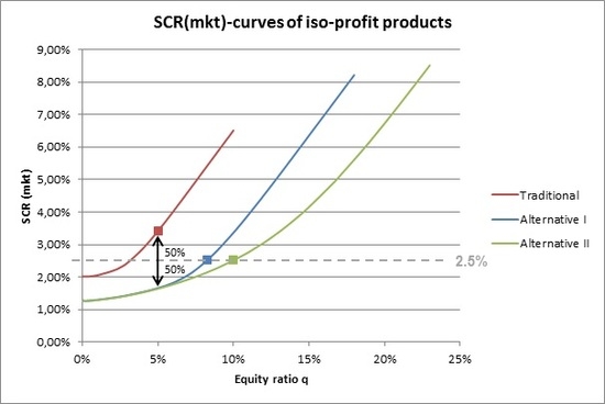
Figure 2 shows
for the iso-profit products from
Figure 1. Note that the
x-axis here only shows the equity ratio
. As explained in the previous subsection, this value
also defines the value of
for the corresponding iso-profit products. Therefore, for a given value of
, the corresponding value of
is different for the three products. We can observe that all three products require more solvency capital with an increasing equity ratio.
If we intend to design products with the same profitability and the same equity ratio, the alternative products will significantly reduce the insurer’s risk. For instance, if we keep the expected profit unchanged at 3.62% and we keep the equity ratio unchanged at 5%, the risk (measured by
) is reduced from 3.41% (for the traditional product) to 1.66% or 1.64% for Alternatives 1 or 2, respectively. Note that in this case, the alternative products come with a higher participation rate (91.48%) than the traditional product (as explained in the previous subsection and
Figure 1). We would like to stress again that these alternative products—when compared to the traditional product—come with the same profitability for the insurer and hence have the same fair value (and the same maturity guarantee) from the policyholder’s perspective. Still, they significantly reduce the insurer’s capital requirement. Of course, products without guarantees at all or with a lower guaranteed benefit at maturity could further reduce the insurer’s risk (measured by
). However, such products would not be attractive to the (large) share of risk averse policyholders that typically seek a certain level of protection. Therefore, we do not consider such products in this paper.
We can also see from
Figure 2 that the alternative products allow for a significantly higher equity ratio if we consider products with identical profitability and identical risk.
4.3. Analysis of Policyholder’s Risk-Return Profiles
Now, we compare the different product designs from a policyholder‘s perspective using risk-return profiles,
22 cf. Graf
et al. [
29]. For this, we perform projections under the real-world measure
(including annual new business of 1000 new policies per year) and analyze the policyholder‘s risk and return on the policies taken out in the first year.
Following typical practice in the German market,
23 the policyholders‘ return is measured by the internal rate of return (IRR) and the policyholders‘ risk is measured by the conditional tail expectation of the return on the lowest 20% of scenarios (CTE20).
As a reference point, we again use the traditional product with and . From an insurer’s perspective, this product has an expected profit of 3.62% and a Solvency Capital Requirement for market risk of about 3.4%.
As in the previous subsection, we first consider alternative products with the same insurer’s profitability and the same asset allocation (which significantly reduce the insurer’s risk, as stated before). The risk-return characteristics from the policyholder’s perspective are shown in
Table 4 (in row “Same asset allocation”). While the expected return barely changes (2.49% for the traditional and 2.47/2.48% for the two alternative products), the CTE20 is reduced from 1.96% to 1.83%. So, from the policyholder’s perspective, such alternative products appear less attractive than the traditional product: they come with a slightly lower return and a moderately increased risk.
24Since iso-profit products that strongly reduce the insurer’s risk do not seem very attractive from the policyholder’s perspective, we now consider iso-profit products that have the same risk from the insurer’s perspective as the traditional product. Such products are identified by the dashed horizontal line in
Figure 2. With Alternative 1 and 2 products, the equity ratio
can be increased to 10.0% and 13.0%, respectively. The corresponding values for
are 90.45% and 89.98%, respectively.
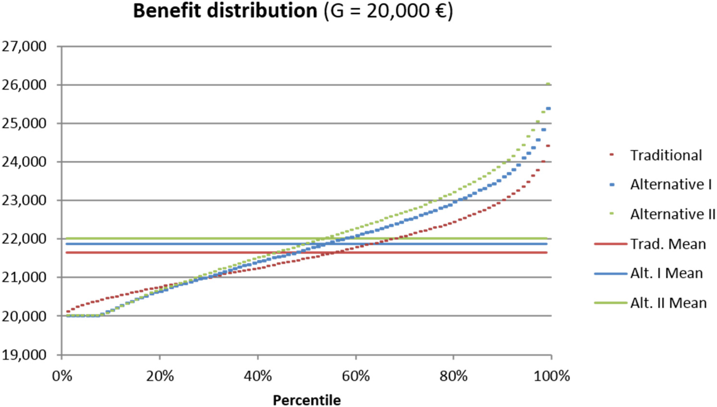
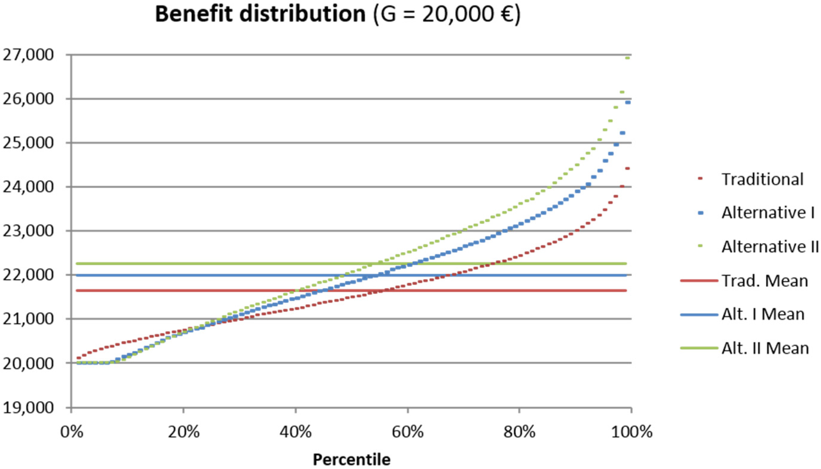
Figure 3 shows the probability distribution of the policyholder’s terminal benefit of these products. We can see that, roughly up to the 25th percentile, the traditional product yields higher benefits than the alternative products. This results from the fact that in adverse years, the traditional product provides higher returns due to the year-by-year cliquet-style guarantees. Moreover, there are some scenarios where the alternative products only pay the guaranteed benefit, which is essentially impossible for the traditional product. For instance, in the fifth percentile, the alternative products pay only the guaranteed benefit of 20,000 €, whereas the traditional product pays 20,314 €. On the other hand, the alternative products provide a higher return in most scenarios. For instance, in the 50th percentile, the payoff of the traditional product is 21,490 € whereas it amounts to 21,848 € or 22,060 € for the alternative products, respectively. In the 95th percentile, the alternative products even pay 1,120 € or 1,817 € more than the traditional product. Also, the mean payoff is higher for the alternative products.
The risk-return characteristics of these products are summarized in
Table 4 (in row “Same risk level”). It demonstrates that the traditional product comes with a lower risk for the policyholder (CTE20 is larger), but the alternative products provide significantly higher expected returns. The increase in risk appears rather small when compared to the increase in expected return by 16 and 26 bps, respectively. This could be due to the fact that a policyholder of an alternative product only receives less than a policyholder of the traditional product if one or several “bad” years occur. On the other hand, such bad years are the key driver for the insurer’s solvency capital requirement. The pure possibility to give less to the policyholder in such bad years reduces the capital requirement, even if no such years occur.
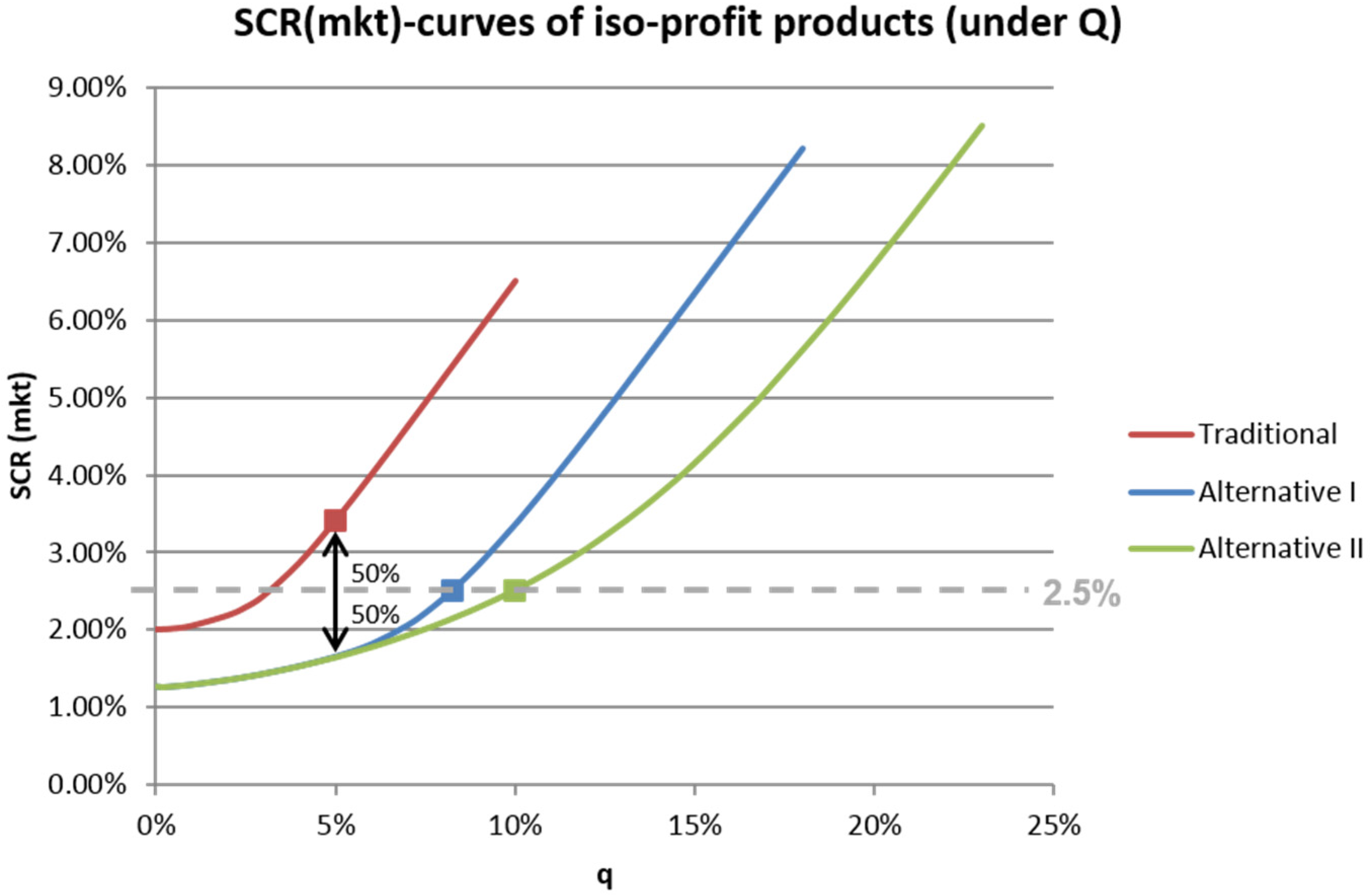
We have now analyzed alternative products that appear very attractive for the insurer but might not appeal to policyholders, and also alternative products that come with interesting risk-return characteristics from the policyholder’s perspective but do not reduce the insurer’s risk. Since the insurer’s primary incentive to develop alternative guarantees is de-risking, the latter would not be appealing to the insurer. We therefore consider alternative product designs that lie between these extremes. We still assume that the insurer designs the products such that the expected profitability (and hence the fair value from the policyholder’s perspective) remains unchanged. However, only 50% of the reduction in risk that would result from a pure modification of guarantees (with unchanged asset allocation) is “given back” to the client in the form of a higher equity ratio and hence more upside potential. This is illustrated on
Figure 4. The alternative products with unchanged profitability and unchanged equity ratio would reduce the
from 3.4% to about 1.65%. Now, we increase the equity ratio such that the resulting products come with 50% of this reduction,
i.e., an
of about 2.5%. The corresponding equity ratios are 8.25% or 10.0%, for Alternative 1 and 2 products, respectively.
Figure 5 shows the benefit distribution of the resulting products from the policyholder’s perspective. We can see that these products, which leave the insurer’s profitability unchanged and provide a significant reduction of the insurer’s risk, provide higher benefits for the policyholder in most scenarios. Again, the alternative products’ benefits are below the traditional product’s benefit only up to the 25th to 28th percentile. Due to the guaranteed maturity benefit that is the same for all three products, however, the difference is limited.
Compared to the previous case where the insurer’s risk was the same for all products, naturally, the expected returns of the alternative products are smaller here (see last row of
Table 4). Compared to the traditional product however, they are still remarkably larger by 10 and 17 bps, respectively. The CTE20 of the alternative products does not change significantly between the two latter risk levels.
25 Therefore, these products might be attractive to both the insurer and the policyholder.
Of course, we cannot conclude that the alternative products would be more beneficial for both the policyholder and the insurer under every measure. Our results are possible since insurers and policyholders focus on different risk measures. Solvency regulation makes insurers focus on market consistent valuation and corresponding risk-based capital requirements whilst regulation with respect to product information disclosure for the policyholder highlights a CTE-measure of the real-world benefit distribution.
4.4. Sensitivity Analyses
In the remainder of this section, we will explain the results of several sensitivity analyses.
4.4.1. Asset Allocation
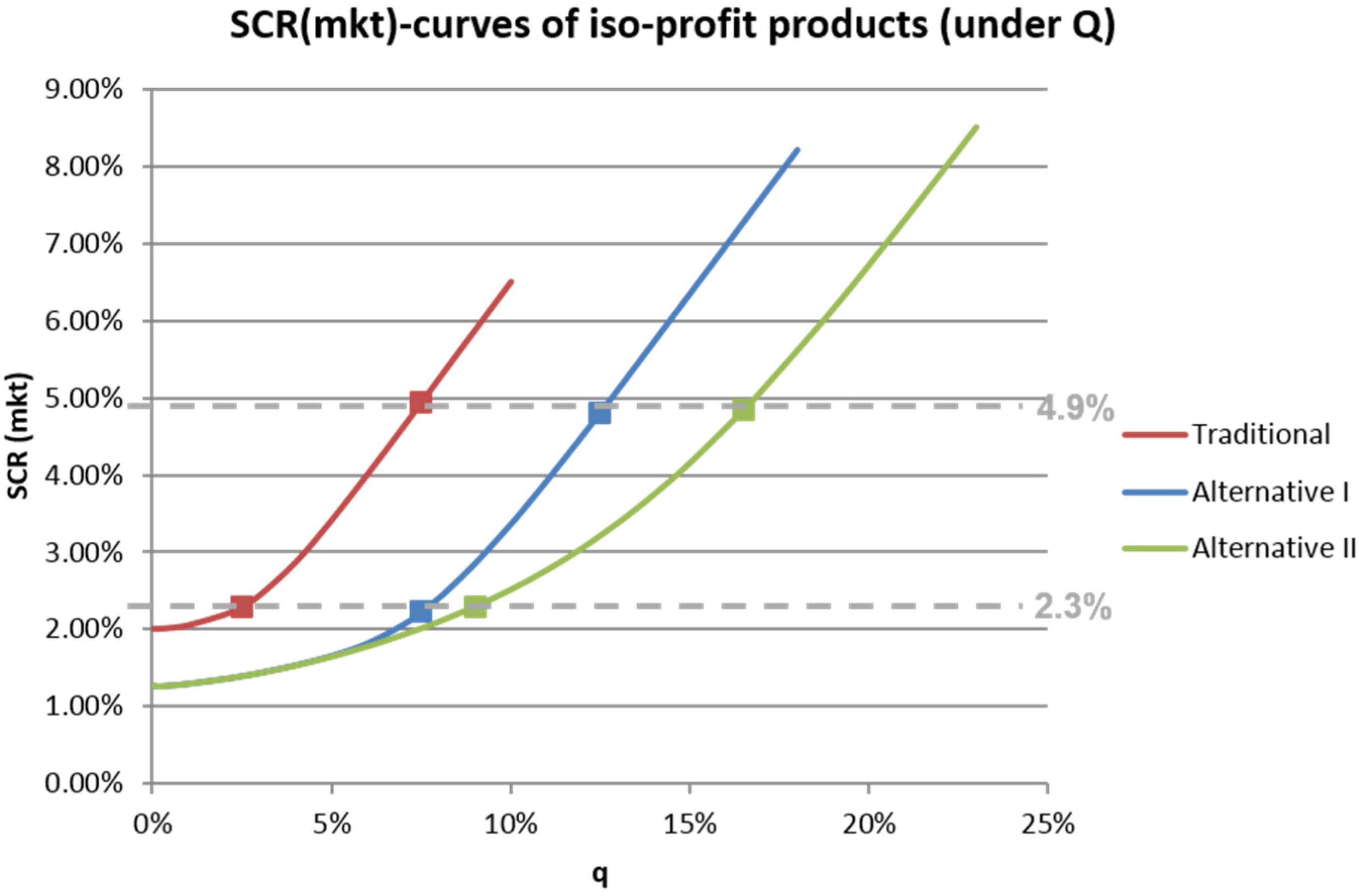
We first perform our analyses for product designs with different asset allocations. We still keep the profitability fixed at a PVFP of 3.62%. For this, we compare traditional products with
(resulting in a
of 2.3%), as well as with
(which implies a
of 4.9%) with alternative products with the same profit and risk level.
Figure 6 shows that in the case of
, the equity ratios can be increased from 2.5% to 7.5% or 9.5% for Alternative 1 and 2, respectively; in the case of
, they increase from 7.5% to 12.5% or 16.5%, respectively.
The values marked “Same risk level” in
Table 5 show the risk-return characteristics of these products from the policyholder’s perspective. We can observe that a higher equity ratio (and thus higher risk for the insurer) leads to a higher expected return from a policyholder perspective and
vice versa. However, the alternative products always provide a significant additional expected return. For all three considered asset allocation levels (base case and sensitivities), the additional expected return is approximately 15 bps for Alternative 1, and between 21 and 30 bps for Alternative 2. Hence, as one would expect, Alternative 2 is more sensitive with respect to the equity ratio level.
It is worth noting that the CTE20 of the traditional product increases significantly with a larger equity ratio, while there is no difference for Alternative 2 and only a slight difference for Alternative 1.
We also performed the analyses for the case that only 50% of the risk reduction is “given back” to the policyholder which in the “less equity” sensitivity leads to an
of 1.8% for the alternative products. They come with equity ratios of 6.0% and 6.25%, respectively. In the “more equity” case,
amounts to 3.5%, and equity ratios increase to 10.25% or 13.25%, respectively. The resulting risk-return profiles (
cf. rows marked “Reduced risk for Alternatives 1/2” in
Table 5) are consistent with the previous observations: As expected, the expected return is lower than in the “Same risk level” case, but still significantly higher than for the traditional product (by approximately 10 bps for Alternative 1, and between 11 and 20 bps for Alternative 2).
4.4.2. Capital Market Assumptions
We now perform analyses for different interest rate levels and expected returns on equity investment: the parameters
,
and
(as defined in
Section 3) are simultaneously reduced or increased by 50 bps. As a reference point, we again use the traditional product with
and
.
In the case of lower capital market returns, the PVFP amounts to 2.48% and comes with an
of 4.71%. If the insurer intends to keep the same profit and the same risk for Alternatives 1 and 2, the equity ratio can be increased to 10.75% or 13.5%, respectively. If the insurer intends to keep the same profit, but to reduce the risk to 3.6% (again by “giving back” 50% of the risk reduction), the equity ratio can be increased to 8.5% or 10.25%, respectively. The resulting risk-return profiles for the policyholder are summarized in
Table 6.
Given the same risk for the insurer, the expected returns of the Alternative 1 and 2 products are 14 or 23 bps higher than for the traditional product. In case of a reduced , the increase is still 7 or 13 bps. The CTE20 is always 9 bps lower.
In the case of higher capital market returns, the starting point corresponds to a PVFP of 4.43% and an of 2.65%. For unchanged risk level, the resulting equity ratios for Alternatives 1 and 2 are 9.5% and 12.5%, respectively. Assuming a reduced of 2.0% (again according to the method outlined above), the equity ratios are 8.0% or 9.75%. The risk-return profiles show additional expected returns for the alternative products of between 11 and 27 bps. Overall, the results for different capital market assumptions prove to be consistent with the base case.
5. Conclusions and Outlook
In this paper, we have discussed profitability and risk of participating products with alternative guarantees, both from the policyholder’s and the insurer’s perspectives. We have considered three different product designs: a traditional product with year-to-year cliquet-style guarantees which is common in Continental Europe, and two products with alternative guarantees. In Reuß
et al. [
13], it has already been shown that such modified guarantees significantly improve the insurer’s profitability while reducing solvency capital requirements. However, in order to keep the alternative products attractive in a market where traditional products continue to be offered, it is expected that the policyholder would demand an additional benefit as a compensation for the somewhat weaker alternative guarantees.
In our analyses we have shown that surplus participation rate and asset allocation of the different products can be adjusted such that all products result in the same profitability from the insurer’s perspective (and hence in the same fair value from the policyholder’s perspective). Even on the same profitability level, the alternative products are significantly less risky from the insurer’s perspective (if the insurer’s asset allocation is not changed) and hence require less solvency capital. If we allow for a change of the asset allocation, products can be designed where the insurer’s risk lies anywhere between this reduced risk and the risk of the traditional product—still without changing the insurer’s profitability or the fair value from the policyholder’s perspective. Nevertheless, the products differ significantly with respect to the risk-return profiles from the policyholder’s perspective.
Since the primary incentive for the insurer to develop products with alternative guarantees is de-risking, products with the same profitability and the same risk are probably not desired. On the other hand, products with alternative guarantees that come with the same profitability and the same asset allocation are significantly less risky from the insurer’s perspective, but appear to be less attractive from the policyholder’s perspective. Therefore, we have focused on product designs that lie between these two cases. If, e.g., 50% of the reduction in risk that would result from a pure modification of guarantees is “given back” to the policyholder by increasing the equity ratio, the policyholder has a significantly higher expected return than with the traditional product design, whereas the policyholder’s risk is only moderately increased. Sensitivity analyses show that similar effects can be achieved also in different capital market environments.
So far, we have separately analyzed portfolios of the traditional or the alternative products. For further research, it would be particularly interesting to see how such products interact when they are combined in an insurer’s book of business: e.g., it might be interesting to investigate the effects on the profitability and risk of an insurer that has sold the traditional product in the past and starts selling alternative products now.
26 Furthermore, we have focused on risk-return profiles to assess the policyholders’ view in this paper. An extension to utility-based analyses also seems worthwhile. Here, at least two questions seem interesting: Which product design (fulfilling certain restrictions defined by the insurer) maximizes utility for a certain type of policyholder?
27 To which type of policyholder (characterized by a utility function and parameters) would a certain product be most appealing? Finally, it would be interesting to analyze how alternative guarantees can be integrated in the annuity payout phase.
In conclusion, products with alternative guarantees allow for a large variety of product designs that might be suitable for reconciling policyholder’s and insurer’s interests, in particular, in a market environment with low interest rates. Hence, when designed properly, participating products with modified guarantees could be of interest to all market participants.


