Ruin Analysis of a Discrete-Time Dependent Sparre Andersen Model with External Financial Activities and Randomized Dividends

Abstract

We consider a discrete-time dependent Sparre Andersen risk model which incorporates multiple threshold levels characterizing an insurer’s minimal capital requirement, dividend paying situations, and external financial activities. We focus on the development of a recursive computational procedure to calculate the finite-time ruin probabilities and expected total discounted dividends paid prior to ruin associated with this model. We investigate several numerical examples and make some observations concerning the impact our threshold levels have on the finite-time ruin probabilities and expected total discounted dividends paid prior to ruin.

1. Introduction

The classical Cramér–Lundberg model is a foundational mathematical representation of an insurer’s surplus process in risk theory. Despite its tractability, however, the model has limitations in terms of applications. Certainly, more complex models are desirable in modern industrial settings. This paper strives to contribute to the ever-growing literature on insurance risk models that reflect more general and realistic modelling approaches to ruin theory.

Bruno de Finetti [1] first introduced the notion of a dividend strategy and the idea of finding an optimal dividend payment strategy for the insurance risk model. This was followed by numerous other researchers who further explored the problem in a variety of contexts (for reviews of the area, the interested reader is directed to Albrecher and Thonhauser [2] and Avanzi [3]). In particular, Drekic and Mera [4] considered the ruin analysis of a threshold-based dividend payment strategy in a discrete-time Sparre Andersen model. Their analysis was an extension of the work by Alfa and Drekic [5], in which a Sparre Andersen insurance risk model in discrete time was analyzed as a doubly-infinite Markov chain to establish a computational procedure for calculating the joint probability distribution of the time of ruin, the surplus immediately prior to ruin, and the deficit at ruin.

In this paper, we focus on the development of a recursive computational procedure to calculate the finite-time ruin probabilities and expected total discounted dividends paid prior to ruin associated with a model which generalizes the single threshold-based risk model introduced by Drekic and Mera [4]. In actual fact, three additional threshold levels are introduced to depict a minimum surplus level control strategy and external financial activities related to both investment and loan undertakings. Readers are referred to, for example, Cai and Dickson [6] and Li [7] for other general investment strategies found in insurance risk models, where the latter paper examined an insurance risk model with risky investments under the assumption that the risky assets follow a Wiener process, and the former paper considered a Markov chain based interest rate model. Korn and Wiese [8] studied optimal investment strategies in an insurance risk model where they also assumed that the risky assets follow a Wiener process.

The remainder of the paper is organized as follows. In Section 2, we introduce notation and specify the fundamental components underlying our threshold-based risk model. Section 3 details the derivation of a recursive formula (namely, Equation (9)) for the finite-time ruin probability associated with our proposed risk model and demonstrates the simplification of the result to that of Drekic and Mera [4]. Section 4 presents the derivation of a similar recursive formula (namely, Equation (13)) to compute the expected total discounted dividends paid prior to ruin and likewise demonstrates the simplification of the result to that of Drekic and Mera [4]. Finally, Section 5 discusses some numerical examples and related findings.

2. Model Description and Assumptions

For $t\in \mathbb{N}$ (with $\mathbb{N}$ being the set of non-negative integers), we define $U_t$ as the insurer’s amount of surplus at time t (measured in discrete monetary units) and $F_t$ as the amount of funds present at time t in the external fund of the insurer, a separate monetary account the insurer holds to better manage its reserve through both investment activities and loan undertakings. In actual fact, $U_t$ represents the surplus level at the end of the time interval $(t-1,t]$, $t\in {\mathbb{Z}}^{+}$ (with ${\mathbb{Z}}^{+}$ being the set of positive integers), at which point any premiums, deposits, claims, or withdrawals corresponding to this time interval have been received/paid out. We adopt the convention that premiums are received at ${(t-1)}^{+}$ and any claims are applied at $t^{-}$.

In what follows, we assume that it is the insurer’s policy to pay out all the outstanding debt before resuming investment activities, and that the insurer first utilizes its investment assets to make any adjustments to its surplus level before engaging in loan activities. To differentiate between investment activities and loan activities with respect to the external fund, we split the support set of $\{F_t,t\in \mathbb{N}\}$ into two disjoint sets, namely $F_t\in (0,\infty )$ and $F_t\in [\beta ,0]$, where β is a non-positive integer representing the minimum support value of $\{F_t,t\in \mathbb{N}\}$. In fact, β is one of four threshold levels we feature in our model with the understanding that $-\beta$ represents the borrowing limit of the insurer. When $F_t>0$, $F_t$ represents the insurer’s investment activities in which interest is assumed to be earned at a constant rate of ${\kappa }_1>0$ per period. Conversely, when $\beta \le F_t\le 0$, $F_t$ represents the insurer’s loan activities and interest expense accumulates at a constant rate of ${\kappa }_2>0$ per period.

We next introduce the remaining three threshold levels (to be denoted by ${\ell }_1$, ${\ell }_2$, and ${\ell }_3$) and explain how they, along with β, define our risk model. To aid in the understanding, let $U_{t^{-}}$ and $F_{t^{-}}$ represent the surplus and external fund levels, respectively, immediately after a claim instance but before a withdrawal instance. Herein, withdrawal refers to any cash inflow from the external fund to the surplus process (whereas deposit refers to any cash outflow from the surplus process to the external fund). Firstly, the threshold ${\ell }_1$ represents the insurer’s minimum acceptable surplus level, and if $U_{t^{-}}$ (corresponding to the time interval $(t-1,t]$) is below ${\ell }_1$ due to a claim, we withdraw or borrow from $F_{t^{-}}$ to bring $U_{t^{-}}$ up to level ${\ell }_1$. However, if $F_{t^{-}}=\beta$, then we can neither withdraw nor borrow more from $F_{t^{-}}$ even if $U_{t^{-}}$ is below ${\ell }_1$. In addition, if $F_{t^{-}}$ (corresponding to the time interval $(t-1,t]$) drifts below β due to interest expense accumulation, we use $U_{t^{-}}$ to pay back the difference at $t^{-}$ as a form of deposit so that $F_t$ is at least kept at its minimum support value of β.

On the other hand, ${\ell }_2$ is a trigger point for investment activities. If $U_t\ge {\ell }_2$, a constant deposit of size d is paid to the external fund at $t^{+}$. Note that the deposit and withdrawal amounts are also stochastic in the sense that they are dependent on the surplus process, and that a deposit can be made at both the left and right limits of a time interval. We denote the left limit deposit amount corresponding to the time interval $(t,t+1]$ to be $D_{1,t}$, the right limit deposit amount corresponding to the time interval $(t-1,t]$ to be $D_{2,t}$, and the withdrawal amount corresponding to the time interval $(t-1,t]$ to be ${\mathcal{W}}_t$.

Lastly, as in Drekic and Mera [4], if $U_t\ge {\ell }_3$, a random dividend is paid out to shareholders at $t^{+}$. We denote the random dividend paid at time t by ${\mathcal{D}}_t$ and assume that $\{{\mathcal{D}}_t,t\in \mathbb{N}\}$ is a conditionally independent and identically distributed (iid) sequence of random variables given $\{U_t,t\in \mathbb{N}\}$. As a final requirement, we assume that ${\ell }_1\le {\ell }_2\le {\ell }_3$.

To sum up, premiums and left limit deposits corresponding to the time interval $(t,t+1]$, $t\in \mathbb{N}$, are collected and paid out at $t^{+}$ according to the following respective (random) rates:

$$P_t=\left\{\begin{array}{cc}c\hfill & \text{if} U_t<{\ell }_3,\hfill \\ X_t\hfill & \text{if} U_t\ge {\ell }_3,\hfill \end{array}\right.$$

and

$$D_{1,t}=\left\{\begin{array}{cc}0\hfill & \text{if} U_t<{\ell }_2,\hfill \\ d\hfill & \text{if} U_t\ge {\ell }_2,\hfill \end{array}\right.$$

where $X_t=c-{\mathcal{D}}_t$ and $b_i=Pr\{X_t=i\}$, $i=c_1,c_1+1,\dots ,c_2$, denotes the probability mass function (pmf) of $X_t$. We refer to $c\in {\mathbb{Z}}^{+}$ as the pure (constant) premium and assume that $c_1,c_2\in \{d,d+1,\dots ,c\}$ where $d\le c$, $c_1\le c_2$, and ${\sum }_{i=c_1}^{c_2}{b}_i=1$. Clearly, $c_1$ and $c_2$ are the respective lower and upper support values of the distribution of the random premium amount $X_t$. Note that, by assumption, the probability distribution of $X_t$ is identical for all values of $t\in \mathbb{N}$. Let $\mu =E\left\{X_0\right\}$ denote the common mean.

Withdrawals and right limit deposits corresponding to the time interval $(t-1,t]$, $t\in {\mathbb{Z}}^{+}$, are made at $t^{-}$ according to the following respective (random) rates:

$${\mathcal{W}}_t=\left\{\begin{array}{cc}0\hfill & \text{if} U_{t^{-}}\ge {\ell }_1,\hfill \\ \text{min}\{{\ell }_1-U_{t^{-}},\text{max}\{0,F_{t^{-}}-\beta \}\}\hfill & \text{if} U_{t^{-}}<{\ell }_1,\hfill \end{array}\right.$$

and

$$D_{2,t}=\text{max}\{0,\beta -F_{t^{-}}\}.$$

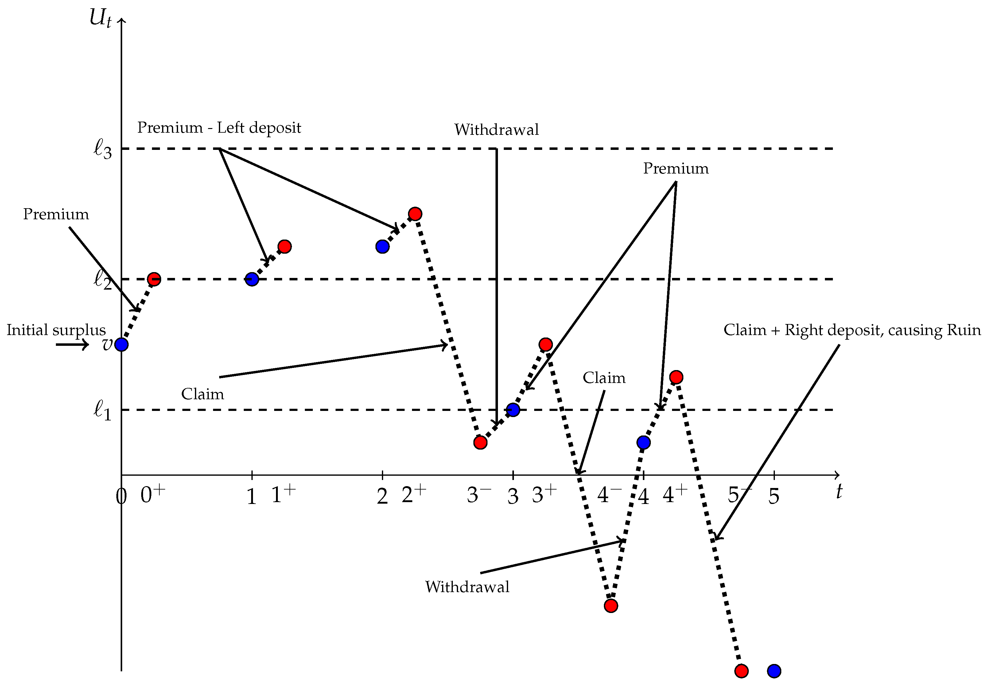
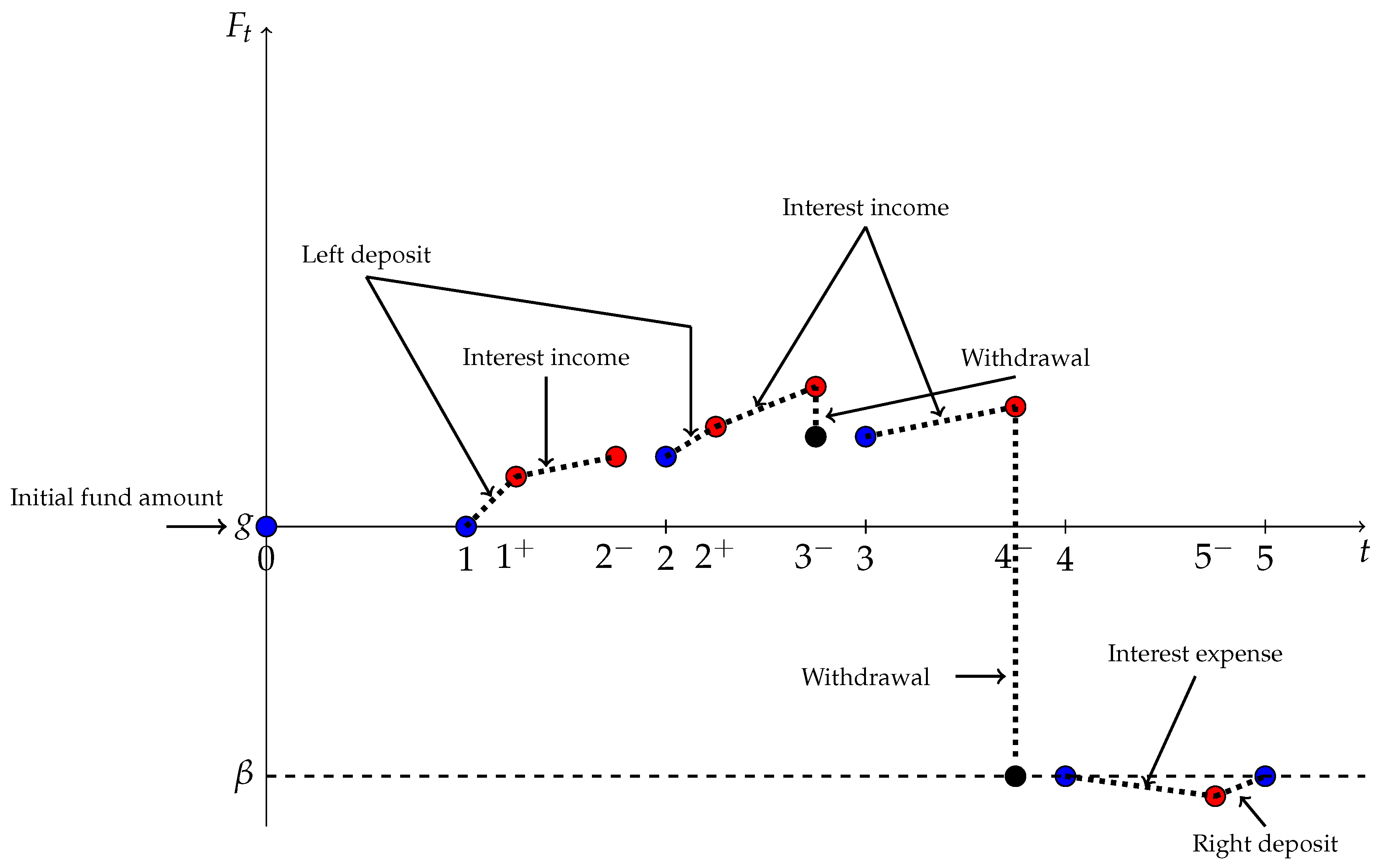
For illustrative purposes, Figure 1 and Figure 2 depict an example of the simultaneous evolution of both the surplus process and that of the external fund.

Figure 1. Sample evolution of the surplus process $\{U_t,t\in \mathbb{N}\}$.

Figure 1. Sample evolution of the surplus process $\{U_t,t\in \mathbb{N}\}$.

Figure 2. Sample evolution of the external fund process $\{F_t,t\in \mathbb{N}\}$.

Figure 2. Sample evolution of the external fund process $\{F_t,t\in \mathbb{N}\}$.

Beginning at time 0 with an initial surplus level of $v\in \{{\ell }_1,{\ell }_1+1,\dots \}$ and an initial external fund amount of $g\in \mathbb{N}$, the insurer’s amount of surplus at time t is expressible as

$$\begin{array}{c}\hfill U_t=v+\sum _{i=0}^{t-1}{P}_i-\sum _{i=0}^{t-1}{D}_{1,i}+\sum _{i=1}^t{\mathcal{W}}_i-\sum _{i=1}^t{D}_{2,i}-\sum _{i=1}^{N_t}{Y}_i,t\in \mathbb{N},\end{array}$$

(1)

where $N_t$ is the number of claims occurring by time t and individual claim sizes $\{Y_i,i\in {\mathbb{Z}}^{+}\}$ are assumed to form an iid sequence of positive, integer-valued random variables. We assume that the number of claims process is a discrete-time renewal process with independent, positive, integer-valued interclaim times $\{W_i,i\in {\mathbb{Z}}^{+}\}$, where $W_i$ is the time between the $(i-1)$-th and i-th claims (with the understanding that the 0-th claim occurs at time 0). In particular, $\{W_i,i\in {\mathbb{Z}}^{+}\}$ forms an iid sequence of positive random variables with common pmf $a_k=Pr\{W_i=k\}$, $k=1,2,\dots ,n_a$ where $n_a\in {\mathbb{Z}}^{+}$, and corresponding survival function $A_k=Pr\{W_i>k\}=1-{\sum }_{j=1}^k{a}_j$. Furthermore, we assume that the pairs $\{(W_i,Y_i),i\in {\mathbb{Z}}^{+}\}$ are iid, so that the joint pmf of $(W_i,Y_i)$ is given by

$$Pr\{W_i=k,Y_i=j\}=a_k{\alpha }_j\left(k\right),$$

where ${\alpha }_j\left(k\right)=Pr\{Y_i=j|W_i=k\}$ denotes the conditional pmf of $Y_i$ given $W_i$. Such a structurization allows for possible dependence between interclaim times and claim sizes in Sparre Andersen models (e.g., see Cheung et al. [9]).

3. Calculation of Finite-Time Ruin Probabilities

We begin by examining the finite-time ruin probabilities associated with the risk model defined by Equation (1). To start with, ruin occurs if and only if $U_t<0$ for some $t\in {\mathbb{Z}}^{+}$ and we denote T to be the time of ruin. In other words, $T=\text{min}\{t\in {\mathbb{Z}}^{+}|U_t<0\}$ with $T=\infty$ if $U_t\ge 0$∀$t\in {\mathbb{Z}}^{+}$.

In what follows, we are interested in computing the quantity

$$\begin{array}{c}\hfill \Psi (v,g,n)=Pr\{T\le n|U_0=v,F_0=g\}=1-Pr\{T>n|U_0=v,F_0=g\},n\in \mathbb{N},\end{array}$$

which we refer to as the finite-time ruin probability. To aid in the computation of this quantity, we introduce the following related function:

$$\begin{array}{c}\hfill \sigma (u,f,n,m)=Pr\{T>n|U_0=u,F_0=f,M_0=m\},n\in \mathbb{N},u\in \mathbb{Z},f\in \{\beta ,\beta +1,\cdots \},\end{array}$$

where $\mathbb{Z}$ denotes the set of all integers and $M_t$, referred to as the elapsed waiting time counter, represents the elapsed time at time t since the most recent claim occurrence and its values lie in the set $\{0,1,\dots ,n_a-1\}$. With the introduction of this function, we remark that $\Psi (v,g,n)=1-\sigma (v,g,n,0)$.

First of all, assuming the occurrence of no claims and no right limit deposits, we need to identify when $U_t\ge {\ell }_2$ and $U_t\ge {\ell }_3$ for the first time. We introduce two functions to denote these time points, namely:

$$z_{t,u}=\left\{\begin{array}{cc}0\hfill & \text{if} u\ge {\ell }_2,\hfill \\ \text{min}\{\lfloor \frac{{\ell }_2-u-1}{c}\rfloor +1,t\}\hfill & \text{if} u<{\ell }_2,\hfill \end{array}\right.$$

and

$$z_{t,u}^{\prime }=\left\{\begin{array}{cc}0\hfill & \text{if} u\ge {\ell }_3,\hfill \\ \text{min}\{\lfloor \frac{{\ell }_3-u-c{z}_{t,u}-1}{c-d}\rfloor +z_{t,u}+1,t\}\hfill & \text{if} u<{\ell }_3,\hfill \end{array}\right.$$

where $\lfloor x\rfloor$, referred to as the floor function of x, yields the largest integer less than or equal to x.

To aid us in obtaining a mathematical expression for $\sigma (u,f,n,m)$, we have to examine how the process $\{F_t,t\in \mathbb{N}\}$ evolves over time. Let us first assume that there are no claims or withdrawals to consider. Clearly, $F_t$ is a non-decreasing function of t if $f\in \mathbb{N}$. On the other hand, if $f\notin \mathbb{N}$, $F_t$ could either be a strictly decreasing function of t or perhaps a convex function depending on the values of f, ${\kappa }_2$ and d. Consequently, if $F_t$ drifts below β, a deposit is forced to be made and this may cause ruin. Thus, in this model, ruin can occur due to either a claim or a deposit. This certainly adds more complexity in deriving a formula for $\sigma (u,f,n,m)$, and as a result, we have to introduce a few more functions. One such function is denoted by $o_{t,u,f}$, representing the time point $s\in \{1,2,\dots ,t\}$ at which $F_s$ is set to become greater than or equal to 0 for the first time. Obtaining this value is not difficult since, assuming the occurrence of no claims and that $F_s\ge \beta$ $\forall s\le o_{t,u,f}$, $F_s$ becomes non-stochastic, the form of which we denote by:

$${\tilde{F}}_{s,u,f}=\left\{\begin{array}{cc}f{(1+{\kappa }_2)}^s+d_{z_{s,u},s}^{{\kappa }_2}\hfill & \text{if} f<0,\hfill \\ f{(1+{\kappa }_1)}^s+d_{z_{s,u},s}^{{\kappa }_1}\hfill & \text{if} f\ge 0,\hfill \end{array}\right.$$

where $d_{k,l}^{{\kappa }_i}$, $k,l\in \mathbb{N}$, represents the future value of deposits made at times $k^{+},{(k+1)}^{+},\dots ,{(l-1)}^{+}$ with respect to interest rate ${\kappa }_i$ per period, $i=1,2$. Clearly, we have $d_{k,l}^{{\kappa }_i}=0$ for $l\le k$ and

$$\begin{array}{c}\hfill d_{k,l}^{{\kappa }_i}=d{(1+{\kappa }_i)}^{l-k}+d{(1+{\kappa }_i)}^{l-k-1}+\cdots +d(1+{\kappa }_i)=\frac{d(1+{\kappa }_i)[{(1+{\kappa }_i)}^{l-k}-1]}{{\kappa }_i},l>k.\end{array}$$

It subsequently follows that

$$o_{t,u,f}=\left\{\begin{array}{cc}t\hfill & \text{if} {\tilde{F}}_{i+1,u,f}<0\forall i\in \{0,1,\dots ,t\},\hfill \\ \text{min}\{i\in \{0,1,\dots ,t\}|{\tilde{F}}_{i+1,u,f}\ge 0\}\hfill & \text{otherwise}.\hfill \end{array}\right.$$

In defining $o_{t,u,f}$ above, we utilize the value of ${\tilde{F}}_{i+1,u,f}$ instead of ${\tilde{F}}_{i,u,f}$. This is because for $f<0$, the function ${\tilde{F}}_{t,u,f},t\in \mathbb{N}$, up-crosses level 0 only if a positive amount of deposit is made to the external fund. We stated earlier that left deposits are made at the left limit point of a discrete-time interval. Thus, ${\tilde{F}}_{i+1,u,f}\ge 0$ for the first time implies that at time $i^{+}$, there was a left deposit made to the external fund.

With the introduction of $o_{t,u,f}$, we henceforth express the non-stochastic form of $F_t$ as

$$\begin{array}{c}\hfill {\widehat{F}}_{t,u,f}=\lfloor (f{(1+{\kappa }_2)}^{o_{t,u,f}}+d_{z_{o_{t,u,f},u},o_{t,u,f}}^{{\kappa }_2}){(1+{\kappa }_1)}^{t-o_{t,u,f}}+d_{\text{max}\{z_{t,u},o_{t,u,f}\},t}^{{\kappa }_1}\rfloor ,t\in \mathbb{N}.\end{array}$$

(2)

Note that Equation (2) involves the use of the floor function to calculate the (non-stochastic) value of the external fund at time t. Such an assumption can be viewed as conservative in nature, since any non-integer value of the external fund (which can arise due to interest accumulation) is essentially rounded down.

There is another important function we introduce next, as it represents the earliest time point when $F_t$ falls below β (again assuming the occurrence of no claims) due to interest expense accumulation. We denote this time point by $c_{t,m,u,f}$ and refer to it as a calling point. It is given by

$$\begin{array}{c}\hfill c_{t,m,u,f}=\left\{\begin{array}{c}\text{min}\{n_a-m,t\}\text{if} {\widehat{F}}_{i,u,f}\ge \beta \forall i\in \{1,2,\dots ,\text{min}\{n_a-m,t\}\},\hfill \\ \text{min}\{i\in \{1,2,\dots ,\text{min}\{n_a-m,t\}\}|{\widehat{F}}_{i,u,f}<\beta \}\text{otherwise}.\hfill \end{array}\right.\end{array}$$

Note that the above function depends on both t and m. As introduced earlier in this section, m represents the elapsed time at time 0 since the most recent claim occurrence.

With these preliminaries in place, we adopt the principle of conditioning on the first claim time as in Cossette et al. [10] or Drekic and Mera [4]. Measured from our initial time point (which we label as time 0), the lower limit of the time until the first claim occurs is 1, but its pmf is now conditional on the value of m. Morever, in evaluating $\sigma (u,f,n,m)$, we condition on first claim times ranging from 1 up to $c_{n,m,u,f}$, and on the event that the time until the first claim occurs is greater than $c_{n,m,u,f}$. For first claim time instances which take place at or before the calling point, the recursive process used is very similar to that of Drekic and Mera [4]. However, in the event that the time until the first claim occurs is greater than $c_{n,m,u,f}$, the recursive process is performed differently. By doing so, we are essentially denoting $c_{n,m,u,f}$ to be the “new” initial time point, updating the parameters of the function σ, and proceeding with the recursive process. We further explain this situation after introducing some necessary boundary conditions for $\sigma (u,f,n,m)$, namely:

$$\sigma (u,f,n,m)=\left\{\begin{array}{cc}0\hfill & \text{if} u\in {\mathbb{Z}}^{-} \text{or} m=n_a,\hfill \\ 1\hfill & \text{if} u\in \mathbb{N},n=0, \text{and} m=0,1,\dots ,n_a-1,\hfill \end{array}\right.$$

(3)

where ${\mathbb{Z}}^{-}$ in Equation (3) denotes the set of negative integers. By conditioning on the events outlined above, we get

$$\begin{array}{cc}\hfill \sigma (u,f,n,m)=& \sum _{k=1}^{c_{n,m,u,f}}\frac{a_{k+m}}{A_m}Pr\{T>n|U_0=u,F_0=f,M_0=m,W_1\left(m\right)=k\}\hfill \\ & +\frac{A_{c_{n,m,u,f}+m}}{A_m}Pr\{T>n|U_0=u,F_0=f,M_0=m,W_1\left(m\right)>c_{n,m,u,f}\},\hfill \end{array}$$

where $W_1\left(m\right)$ is the duration from our initial time point until the first claim occurs given that the elapsed waiting time at time 0 since the most recent claim is m.

At time $k\in \{1,2,\dots ,c_{n,m,u,f}\}$, the elapsed waiting time counter is reset to 0 for the next recursion, n is reduced by k, and the “new” initial surplus and external fund amounts are determined by the size of the incurred claim and the premiums received up to time k. Specifically, we obtain

$$\begin{array}{cc}& Pr\{T>n|U_0=u,F_0=f,M_0=m,W_1\left(m\right)=k\}\hfill \\ \hfill =& \sum _{l=(k-z_{k,u}^{\prime })c_1}^{(k-z_{k,u}^{\prime })c_2}{b}_{l,k-z_{k,u}^{\prime }}\sum _{j=1}^{u+c{z}_{k,u}^{\prime }-d(k-z_{k,u})+l+{\widehat{F}}_{k,u,f}-\beta }{\alpha }_j(k+m)\sigma (u^{*},f^{*},n-k,0),\hfill \end{array}$$

where

$$\begin{array}{cc}\hfill u^{*}=& u+c{z}_{k,u}^{\prime }-d(k-z_{k,u})+l-j\hfill \\ & +\text{min}\{{\widehat{F}}_{k,u,f}-\beta ,\text{max}\{0,j-[u+c{z}_{k,u}^{\prime }-d(k-z_{k,u})+l-{\ell }_1]\}\},\hfill \end{array}$$

(4)

$$\begin{array}{c}\hfill f^{*}=\text{max}\{\beta ,\text{min}\{{\widehat{F}}_{k,u,f},{\widehat{F}}_{k,u,f}-j+[u+c{z}_{k,u}^{\prime }-d(k-z_{k,u})+l-{\ell }_1]\}\},\end{array}$$

(5)

and l denotes the value of the sum of the random premiums received up to time k, with corresponding pmf $b_{l,k-z_{k,u}^{\prime }}$ representing the $(k-z_{k,u}^{\prime })$-fold convolution of $b_l$ with itself. To evaluate the pmf $b_{l,r}$, $r\in \mathbb{N}$, we define $b_{l,0}={\delta }_{l,0}$ (where ${\delta }_{i,j}$, in general, denotes the Kronecker delta function of i and j),

$$\begin{array}{c}\hfill b_{l,1}=\left\{\begin{array}{cc}{b}_l\hfill & \text{if} l=c_1,c_1+1,\dots ,c_2,\hfill \\ 0\hfill & \text{otherwise},\hfill \end{array}\right.\end{array}$$

and for $r=2,3,\dots$,

$$\begin{array}{c}\hfill b_{l,r}=\left\{\begin{array}{cc}\sum _{j=c_1}^{c_2}{b}_{j,1}{b}_{l-j,r-1}\hfill & \text{if} l=r{c}_1,r{c}_1+1,\dots ,r{c}_2,\hfill \\ 0\hfill & \text{otherwise}.\hfill \end{array}\right.\end{array}$$

The reasoning behind the definitions of the above parameters is that we first consider whether the claim size is substantial enough for the surplus process to fall below its minimum support level ${\ell }_1$. If so, then $j-[u+c{z}_{k,u}^{\prime }-d(k-z_{k,u})+l-{\ell }_1]$ is a positive quantity and we consider whether the external fund is able to support the surplus process. We do this by comparing ${\widehat{F}}_{k,u,f}-\beta$ and $j-[u+c{z}_{k,u}^{\prime }-d(k-z_{k,u})+l-{\ell }_1]$, and choosing the minimum of the two quantities to ensure that the external fund does not fall below the maximum level of external funding allowed, β. If $j-[u+c{z}_{k,u}^{\prime }-d(k-z_{k,u})+l-{\ell }_1]$ is a non-positive quantity, then the surplus process is greater than or equal to ${\ell }_1$ after the claim, in which case, we only need to consider whether ${\widehat{F}}_{k,u,f}$ is below β. If so, ${\widehat{F}}_{k,u,f}-\beta$ is less than 0, and we would subtract $|{\widehat{F}}_{k,u,f}-\beta |$ from the surplus process and add it to the external fund to bring it up to β.

In situations when $W_1\left(m\right)>c_{n,m,u,f}$, we perform a recursion at $c_{n,m,u,f}$ to similarly acquire

$$\begin{array}{cc}\hfill & {\displaystyle Pr\{T>n|U_0=u,F_0=f,M_0=m,W_1\left(m\right)>c_{n,m,u,f}\}}\hfill \\ \hfill =& \sum _{l=(c_{n,m,u,f}-z_{c_{n,m,u,f},u}^{\prime })c_1}^{(c_{n,m,u,f}-z_{c_{n,m,u,f},u,f}^{\prime })c_2}{b}_{l,c_{n,m,u,f}-z_{c_{n,m,u,f},u,f}^{\prime }}\sigma (u^{\prime },f^{\prime },n-c_{n,m,u,f},c_{n,m,u,f}+m),\hfill \end{array}$$

(6)

where

$$\begin{array}{c}\hfill u^{\prime }=u+c{z}_{c_{n,m,u,f},u}^{\prime }-d(c_{n,m,u,f}-z_{c_{n,m,u,f},u})+l+\text{min}\{0,{\widehat{F}}_{c_{n,m,u,f},u,f}-\beta \}\end{array}$$

(7)

and

$$\begin{array}{c}\hfill f^{\prime }=\text{max}\{{\widehat{F}}_{c_{n,m,u,f},u,f},\beta \}.\end{array}$$

(8)

We remark that when $W_1\left(m\right)>c_{n,m,u,f}$, there is no claim size to consider at time $c_{n,m,u,f}$. Thus, all we need to account for is whether ${\widehat{F}}_{c_{n,m,u,f},u,f}$ falls below β. In this case, just enough funds would be withdrawn from the surplus process and added to the external fund to bring it up to β. However, note that ${\widehat{F}}_{c_{n,m,u,f},u,f}$ may not necessarily be below β. If ${\widehat{F}}_{c_{n,m,u,f},u,f}\ge \beta$, then $c_{n,m,u,f}=\text{min}\{n_a-m,n\}$ and this implies that either $n-c_{n,m,u,f}=0$ or $c_{n,m,u,f}+m=n_a$ in Equation (6). This yields an interesting outcome. Given that $W_1\left(m\right)\ge c_{n,m,u,f}$ and ${\widehat{F}}_{c_{n,m,u,f},u,f}\ge \beta$, it must be that $u^{\prime }\ge 0$ at time $c_{n,m,u,f}$. However, if $c_{n,m,u,f}+m=n_a$, then $\sigma (u^{\prime },f^{\prime },n-c_{n,m,u,f},n_a)$ is set equal to 0 via Equation (3). On the other hand, if $n<n_a-m$ so that $c_{n,m,u,f}=n$, then $\sigma (u^{\prime },f^{\prime },0,c_{n,m,u,f}+m)=1$ from Equation (3). Putting it altogether, we establish the following final formula for $\sigma (u,f,n,m)$:

$$\begin{array}{cc}\hfill & \sigma (u,f,n,m)\hfill \\ \hfill =& \sum _{k=1}^{c_{n,m,u,f}}\frac{a_{k+m}}{A_m}\sum _{l=(k-z_{k,u}^{\prime })c_1}^{(k-z_{k,u}^{\prime })c_2}{b}_{l,k-z_{k,u}^{\prime }}\sum _{j=1}^{u+c{z}_{k,u}^{\prime }-d(k-z_{k,u})+l+{\widehat{F}}_{k,u,f}-\beta }{\alpha }_j(k+m)\sigma (u^{*},f^{*},n-k,0)\hfill \\ \hfill +& \frac{A_{c_{n,m,u,f}+m}}{A_m}\sum _{l=(c_{n,m,u,f}-z_{c_{n,m,u,f},u}^{\prime })c_1}^{(c_{n,m,u,f}-z_{c_{n,m,u,f},u}^{\prime })c_2}{b}_{l,c_{n,m,u,f}-z_{c_{n,m,u,f},u}^{\prime }}\sigma (u^{\prime },f^{\prime },n-c_{n,m,u,f},c_{n,m,u,f}+m).\hfill \end{array}$$

(9)

Note that the determination of $\sigma (u,f,n,m)$ via Equation (9) requires a double recursion in both n and m, with boundary conditions given by Equation (3) serving as the starting point. Moreover, if we assume that $f=0,d=0,{\ell }_1=0,\beta =0$, $m=0$, and ${\alpha }_j\left(k\right)=Pr\{Y_i=j|W_i=k\}=Pr\{Y_i=j\}={\alpha }_j$ (i.e., $Y_i$ is independent of $W_i$ $\forall i\in {\mathbb{Z}}^{+}$), then the model under consideration is equivalent to the independent Sparre Andersen model studied by Drekic and Mera [4]. To verify this, we first observe that $c_{n,0,u,0}=\text{min}\{n,n_a\}\forall n\in {\mathbb{Z}}^{+}$. If $n<n_a$, then $\sigma (u^{\prime },f^{\prime },0,n)=1$ and

$$\frac{A_n}{A_0}Pr(T>n|U_0=u,F_0=0,M_0=0,W_1\left(0\right)>n)=A_n\sum _{l=(n-z_{n,u}^{\prime })c_1}^{(n-z_{n,u}^{\prime })c_2}{b}_{l,n-z_{n,u}^{\prime }}=A_n.$$

Conversely, if $n\ge n_a$, then $\sigma (u^{\prime },f^{\prime },n-n_a,n_a)=0$ and

$$\frac{A_{n_a}}{A_0}Pr(T>n|U_0=u,F_0=0,M_0=0,W_1\left(0\right)>n_a)=A_{n_a}\times 0=0.$$

Thus, Equation (9) simplifies to become

$$\sigma (u,0,n,0)=A_n+\sum _{k=1}^{\text{min}\{n,n_a\}}{a}_k\sum _{l=(k-z_{k,u}^{\prime })c_1}^{(k-z_{k,u}^{\prime })c_2}{b}_{l,k-z_{k,u}^{\prime }}\sum _{j=1}^{u+c{z}_{k,u}^{\prime }+l}{\alpha }_j\sigma (u+c{z}_{k,u}^{\prime }+l-j,0,n-k,0),$$

which is consistent with the result in Drekic and Mera [4], p. 744.

4. Calculation of Expected Total Discounted Dividend Payments

Our next objective is to derive a corresponding recursive formula to compute the expected total discounted dividend payments made prior to ruin. The approach we employ essentially borrows from that of Dickson and Waters [11], Section 5. Let $E\left\{{\mathcal{D}}_{v,g}\right\}$ denote the expected total discounted (i.e., to time 0 according to discount factor $\nu \in (0,1)$ per unit of time) dividends paid prior to ruin, where the random variable ${\mathcal{D}}_{v,g}$ represents the total discounted dividends paid before ruin starting from an initial surplus of v and an initial level of g in the external fund. Moreover, we also introduce the analogous quantity $E\left\{{\mathcal{D}}_{v,g,n}\right\}$ as the expected total discounted dividends paid before ruin occurs or strictly before time $n\in {\mathbb{Z}}^{+}$, whichever happens first.

In order to calculate $E\left\{{\mathcal{D}}_{v,g}\right\}$, we develop a computational procedure for calculating $E\left\{{\mathcal{D}}_{v,g,n}\right\}$ and then use the fact that $E\left\{{\mathcal{D}}_{v,g,n}\right\}\to E\left\{{\mathcal{D}}_{v,g}\right\}$ as $n\to \infty$. To aid in the computation of $E\left\{{\mathcal{D}}_{v,g,n}\right\}$, we introduce a function (similar in nature to σ from the previous section) defined by

$$\begin{array}{c}\hfill V(u,f,n,m)=E\left\{{\mathcal{D}}_{u,f,n}\right|M_0=m\},n\in {\mathbb{Z}}^{+},u\in \mathbb{Z},f\in \{\beta ,\beta +1,\dots \},m\in \{0,1,\dots ,n_a-1\}.\end{array}$$

Clearly, $E\left\{{\mathcal{D}}_{v,g,n}\right\}=V(v,g,n,0)$. As with the function σ in the previous section, the function $V(u,f,n,m)$ also has its own set of boundary conditions, namely:

$$V(u,f,n,m)=\left\{\begin{array}{cc}0\hfill & \text{if} u\in {\mathbb{Z}}^{-} \text{or} m=n_a,\hfill \\ 0\hfill & \text{if} 0\le u<{\ell }_3 \text{and} n=1,\hfill \\ c-\mu \hfill & \text{if} u\ge {\ell }_3 \text{and} n=1.\hfill \end{array}\right.$$

(10)

We employ a similar approach as in the previous section by conditioning on values of $W_1\left(m\right)$ ranging from 1 up to $c_{n-1,m,u,f}$, as well as the case when $W_1\left(m\right)>c_{n-1,m,u,f}$. By conditioning on these events, we immediately obtain

$$\begin{array}{cc}\hfill & V(u,f,n,m)\hfill \\ \hfill =& \sum _{k=1}^{c_{n-1,m,u,f}}\frac{a_{k+m}}{A_m}E\left\{{\mathcal{D}}_{u,f,n,m}\right|W_1\left(m\right)=k\}+\frac{A_{c_{n-1,m,u,f}+m}}{A_m}E\left\{{\mathcal{D}}_{u,f,n,m}\right|W_1\left(m\right)>c_{n-1,m,u,f}\}.\hfill \end{array}$$

For $k\in \{1,2,\dots ,c_{n-1,m,u,f}\}$, an expected dividend payment of amount $c-\mu$ would occur at times $z_{k,u}^{\prime +},{(z_{k,u}^{\prime }+1)}^{+},\dots ,{(k-1)}^{+}$, followed by possible future dividend payments (starting from time k) once the initial claim is applied. Applying the appropriate conditioning arguments ultimately leads to

$$\begin{array}{cc}\hfill & E\left\{{\mathcal{D}}_{u,f,n,m}\right|W_1\left(m\right)=k\}\hfill \\ \hfill =& \sum _{i=z_{k,u}^{\prime }}^{k-1}{\nu }^i(c-\mu )+{\nu }^k\sum _{l=(k-z_{k,u}^{\prime })c_1}^{(k-z_{k,u}^{\prime })c_2}{b}_{l,k-z_{k,u}^{\prime }}\sum _{j=1}^{u+c{z}_{k,u}^{\prime }-d(k-z_{k,u})+l+{\widehat{F}}_{k,u,f}-\beta }{\alpha }_j(k+m)V(u^{*},f^{*},n-k,0),\hfill \end{array}$$

(11)

where $u^{*}$ and $f^{*}$ are given by Equations (4) and (5), respectively. For $W_1\left(m\right)>c_{n-1,m,u,f}$, however, we need to reset the parameters of the function V as we did in our treatment of the finite-time ruin probabilities and base the recursion at $c_{n-1,m,u,f}$. We also need to account for the expected dividend payments received at times $z_{c_{n-1,m,u,f},u}^{\prime +},{(z_{c_{n-1,m,u,f},u}^{\prime }+1)}^{+},\dots ,{(c_{n-1,m,u,f}-1)}^{+}$. Thus, we eventually obtain

$$\begin{array}{cc}\hfill & {\displaystyle E\left\{{\mathcal{D}}_{u,f,n,m}\right|W_1\left(m\right)>c_{n-1,m,u,f}\}}\hfill \\ \hfill =& \sum _{i=z_{c_{n-1,m,u,f}}^{\prime }}^{c_{n-1,m,u,f}-1}{\nu }^i(c-\mu )+{\nu }^{c_{n-1,m,u,f}}\hfill \\ & \times \sum _{l=(c_{n-1,m,u,f}-z_{c_{n-1,m,u,f},u}^{\prime })c_1}^{(c_{n-1,m,u,f}-z_{c_{n-1,m,u,f},u}^{\prime })c_2}{b}_{l,c_{n-1,m,u,f}-z_{c_{n-1,m,u,f},u}^{\prime }}V(\widehat{u},\widehat{f},n-c_{n-1,m,u,f},c_{n-1,m,u,f}+m),\hfill \end{array}$$

(12)

where

$$\begin{array}{c}\hfill \widehat{u}=u+c{z}_{c_{n-1,m,u,f},u}^{\prime }-d(c_{n-1,m,u,f}-z_{c_{n-1,m,u,f},u})+l+\text{min}\{0,{\widehat{F}}_{c_{n-1,m,u,f},u,f}-\beta \},\end{array}$$

and

$$\begin{array}{c}\hfill \widehat{f}=\text{max}\{{\widehat{F}}_{c_{n-1,m,u,f},u,f},\beta \}.\end{array}$$

Note that $\widehat{u}$ and $\widehat{f}$ are identical in form to Equations (7) and (8), respectively, with n simply replaced by $n-1$. Combining Equations (11) and (12) eventually yields the final overall formula

$$\begin{array}{cc}\hfill & {\displaystyle V(u,f,n,m)}\hfill \\ \hfill =& \sum _{k=1}^{c_{n-1,m,u,f}}\frac{a_{k+m}}{A_m}[(c-\mu )\frac{{\nu }^{z_{k,u}^{\prime }}-{\nu }^k}{1-\nu }\hfill \\ \hfill & +{\nu }^k\sum _{l=(k-z_{k,u}^{\prime })c_1}^{(k-z_{k,u}^{\prime })c_2}{b}_{l,k-z_{k,u}^{\prime }}\sum _{j=1}^{u+c{z}_{k,u}^{\prime }-d(k-z_{k,u})+l+{\widehat{F}}_{k,u}-\beta }{\alpha }_j(k+m)V(u^{*},f^{*},n-k,0)]\hfill \\ \hfill & +\frac{A_{c_{n-1,m,u,f}+m}}{A_m}[(c-\mu )\frac{{\nu }^{z_{c_{n-1,m,u,f},u}^{\prime }}-{\nu }^{c_{n-1,m,u,f}}}{1-\nu }+{\nu }^{c_{n-1,m,u,f}}\hfill \\ & \times \sum _{l=(c_{n-1,m,u,f}-z_{c_{n-1,m,u,f},u}^{\prime })c_1}^{(c_{n-1,m,u,f}-z_{c_{n-1,m,u,f},u}^{\prime })c_2}{b}_{l,c_{n-1,m,u,f}-z_{c_{n-1,m,u,f},u}^{\prime }}V(\widehat{u},\widehat{f},n-c_{n-1,m,u,f},c_{n-1,m,u,f}+m)].\hfill \end{array}$$

(13)

Similar to the function σ of the previous section, we note that the use of Equation (13) requires a double recursion in both n and m, with boundary conditions given by Equation (10) serving as the starting point. As before, we consider the situation when $f=0,d=0,{\ell }_1=0,\beta =0$, $m=0$, and ${\alpha }_j\left(k\right)={\alpha }_j$, so that the model under consideration is equivalent to the one analyzed by Drekic and Mera [4]. In this case, Equation (13) reduces to

$$\begin{array}{cc}\hfill V(u,0,n,0)=& \sum _{k=1}^{\text{min}\{n-1,n_a\}}{a}_k[(c-\mu )\frac{{\nu }^{z_{k,u}^{\prime }}-{\nu }^k}{1-\nu }\hfill \\ \hfill & +{\nu }^k\sum _{l=(k-z_{k,u}^{\prime })c_1}^{(k-z_{k,u}^{\prime })c_2}{b}_{l,k-z_{k,u}^{\prime }}\sum _{j=1}^{u+c{z}_{k,u}^{\prime }+l}{\alpha }_{j}V(u+c{z}_{k,u}^{\prime }+l-j,0,n-k,0)]\hfill \\ \hfill & +A_{\text{min}\{n-1,n_a\}}[(c-\mu )\frac{{\nu }^{z_{n-1,u}^{\prime }}-{\nu }^{n-1}}{1-\nu }\hfill \\ & +{\nu }^{n-1}\sum _{l=(n-1-z_{n-1,u}^{\prime })c_1}^{(n-1-z_{n-1,u}^{\prime })c_2}{b}_{l,n-1-z_{n-1,u}^{\prime }}V(u+c{z}_{n-1,u}^{\prime }+l,0,1,n-1)].\hfill \end{array}$$

(14)

We remark that since $c_{n-1,0,u,0}=\text{min}\{n-1,n_a\}$, the square-bracketed term in Equation (14) that is pre-multiplied by $A_{\text{min}\{n-1,n_a\}}$ matters only if $c_{n-1,0,u,0}=n-1$ since $A_{n_a}=0$. Thus, for convenience, we set $c_{n-1,0,u,0}=n-1$ inside this square-bracketed term in Equation (14). In addition, Equation (14) simplifies further to become:

$$\begin{array}{cc}\hfill & V(u,0,n,0)\hfill \\ & =\left\{\begin{array}{c}{\displaystyle \sum _{k=1}^{\text{min}\{n-1,n_a\}}}{a}_k[(c-\mu )\frac{{\nu }^{z_{k,u}^{\prime }}-{\nu }^k}{1-\nu }\hfill \\ +{\nu }^k{\displaystyle \sum _{l=(k-z_{k,u}^{\prime })c_1}^{(k-z_{k,u}^{\prime })c_2}}{b}_{l,k-z_{k,u}^{\prime }}{\displaystyle \sum _{j=1}^{u+c{z}_{k,u}^{\prime }+l}}{\alpha }_{j}V(u+c{z}_{k,u}^{\prime }+l-j,0,n-k,0)]\hfill & \text{if} z_{n-1,u}^{\prime }<z_{n,u}^{\prime },\hfill \\ \\ {\displaystyle \sum _{k=1}^{\text{min}\{n-1,n_a\}}}{a}_k[(c-\mu )\frac{{\nu }^{z_{k,u}^{\prime }}-{\nu }^k}{1-\nu }\hfill \\ +{\nu }^k{\displaystyle \sum _{l=(k-z_{k,u}^{\prime })c_1}^{(k-z_{k,u}^{\prime })c_2}}{b}_{l,k-z_{k,u}^{\prime }}{\displaystyle \sum _{j=1}^{u+c{z}_{k,u}^{\prime }+l}}{\alpha }_{j}V(u+c{z}_{k,u}^{\prime }+l-j,0,n-k,0)]\hfill \\ +A_{\text{min}\{n-1,n_a\}}{\displaystyle \sum _{i=z_{n-1,u}^{\prime }}^{n-1}}{\nu }^i(c-\mu )\hfill & \text{if} z_{n-1,u}^{\prime }=z_{n,u}^{\prime }.\hfill \end{array}\right.\hfill \end{array}$$

(15)

The logic behind Equation (15) is as follows. If $z_{n-1,u}^{\prime }<z_{n,u}^{\prime }$, then $z_{n,u}^{\prime }=n$. This implies that there are no dividend payments before time n, and hence, Equation (12) becomes equal to 0. On the other hand, if $z_{n-1,u}^{\prime }=z_{n,u}^{\prime }$, then there is a guaranteed dividend payment at time $n-1$ and

$$\begin{array}{c}\hfill \sum _{l=(n-1-z_{n-1,u}^{\prime })c_1}^{(n-1-z_{n-1,u}^{\prime })c_2}{b}_{l,n-1-z_{n-1,u}^{\prime }}V(u+c{z}_{n-1,u}^{\prime }+l,0,1,n-1)=c-\mu .\end{array}$$

Thus, the quantity

$$\begin{array}{c}\hfill A_{\text{min}\{n-1,n_a\}}\sum _{i=z_{n-1,u}^{\prime }}^{n-1}{\nu }^i(c-\mu )\end{array}$$

in the second component of Equation (15) can be rewritten as

$$\begin{array}{c}\hfill A_{n-1}\sum _{i=z_{n,u}^{\prime }}^{n-1}{\nu }^i(c-\mu ).\end{array}$$

In addition, consider the expression

$$\begin{array}{c}\hfill \sum _{k=n}^{n_a}{a}_k\sum _{i=z_{k,u}^{\prime }}^{n-1}{\nu }^i(c-\mu ).\end{array}$$

(16)

If $z_{n,u}^{\prime }=z_{n+1,u}^{\prime }=\dots =z_{n_a,u}^{\prime }$, then certainly we can replace $z_{n+1,u}^{\prime },z_{n+2,u}^{\prime },\dots ,z_{n_a,u}^{\prime }$ with $z_{n,u}^{\prime }$ in Equation (16). Otherwise, $z_{n,u}^{\prime }=n$, and since min$\{z_{n,u}^{\prime },z_{n+1,u}^{\prime },\dots ,z_{n_a,u}^{\prime }\}=z_{n,u}^{\prime }$, Equation (16) evaluates to 0. In either case, Equation (16) becomes

$$\begin{array}{c}\hfill \sum _{k=n}^{n_a}{a}_k\sum _{i=z_{k,u}^{\prime }}^{n-1}{\nu }^i(c-\mu )=\sum _{k=n}^{n_a}{a}_k\sum _{i=z_{n,u}^{\prime }}^{n-1}{\nu }^i(c-\mu )=A_{n-1}\sum _{i=z_{n,u}^{\prime }}^{n-1}{\nu }^i(c-\mu ).\end{array}$$

Substituting these results into Equation (15) and simplifying ultimately yields

$$\begin{array}{cc}\hfill V(u,0,n,0)& =(c-\mu )\sum _{k=1}^{n_a}{a}_k\frac{{\nu }^{\text{min}\{z_{k,u}^{\prime },n\}}-{\nu }^{\text{min}\{k,n\}}}{1-\nu }\hfill \\ & +\sum _{k=1}^{\text{min}\{n-1,n_a\}}{a}_k{\nu }^k\sum _{l=(k-z_{k,u}^{\prime })c_1}^{(k-z_{k,u}^{\prime })c_2}{b}_{l,k-z_{k,u}^{\prime }}\sum _{j=1}^{u+c{z}_{k,u}^{\prime }+l}{\alpha }_{j}V(u+c{z}_{k,u}^{\prime }+l-j,0,n-k,0).\hfill \end{array}$$

Once again, the above formula coincides with that of Drekic and Mera ([4], p. 745).

5. Numerical Results

In this section, we implement our key recursive formulas (namely, Equations (9) and (13)) and investigate the behaviour of our proposed risk model through some numerical examples. To the best of our knowledge, we are unaware of any alternative computational methods to calculate these two ruin-related quantities of interest for the kind of discrete-time risk model considered in this paper. In fact, most methods in the literature have employed conditioning arguments similar to ours to analyze discrete-time risk models and ultimately formulate a recursive procedure to calculate such quantities.

In what follows, we focus specifically on the independent Sparre Andersen model (i.e., ${\alpha }_j\left(k\right)={\alpha }_j$) and introduce a set of interclaim time distributions to study, namely:

$$\begin{array}{cc}& \text{(a)}{a}_j=\left\{\begin{array}{cc}(2/11){(9/11)}^{j-1}\hfill & \text{if} j=1,2,\dots ,24,\hfill \\ {(9/11)}^{24}\hfill & \text{if} j=25,\hfill \end{array}\right.\hfill \\ & \text{(b)}{a}_j=1/10,j=1,2,\dots ,10,\hfill \\ & \text{(c)}{a}_j=\frac{1}{1-{(39/50)}^{25}}\left(\genfrac{}{}{0pt}{}{25}{j}\right){(11/50)}^j{(39/50)}^{25-j},j=1,2,\dots ,25,\hfill \\ & \text{(d)}{a}_j=\left\{\begin{array}{cc}(0.645){(1/2)}^j+(0.355)(1/12){(11/12)}^{j-1}\hfill & \text{if} j=1,2,\dots ,14,\hfill \\ (0.645){(1/2)}^{14}+(0.355)(1/12){(11/12)}^{14}\hfill & \text{if} j=15,\hfill \\ (0.355)(1/12){(11/12)}^{j-1}\hfill & \text{if} j=16,17,\dots ,49,\hfill \\ (0.355){(11/12)}^{49}\hfill & \text{if} j=50.\hfill \end{array}\right.\hfill \end{array}$$

We observe that (a) is the pmf of a truncated geometric distribution with $n_a=25$; (b) is the pmf of a uniform distribution on $\{1,2,\dots ,10\}$; (c) is the pmf of a zero-truncated binomial distribution with $n_a=25$; and (d) is the pmf of a mixture of two truncated geometric distributions with $n_a=50$. We note that the means are essentially equal to 5.5 for all four interclaim time distributions, but their variability differs with (c) being the least variable and (d) being the most variable.

As for the random premium distribution, in effect, we consider a degenerate distribution with all the probability mass on 2 (i.e., $c_1=c_2=2$, so that $b_2=1$). In terms of the claim size distribution, we consider a discretized version of the Pareto distribution with mean 10 and pmf of the form

$$\begin{array}{c}\hfill {\alpha }_j={\left(1+\frac{j-1}{30}\right)}^{-4}-{\left(1+\frac{j}{30}\right)}^{-4},j\in {\mathbb{Z}}^{+}.\end{array}$$

Incidentally, the above claim size pmf results from the application of the “lower bound” discretization method of Dickson ([12], p. 79) to approximate a Pareto distribution which is continuous. In fact, similar discretization ideas (e.g., see Dickson et al. [13] or Alfa and Drekic [5], pp. 306–307) can be employed to construct a discrete-time approximation to a continuous-time analogue of our proposed risk model. We also remark that the above set of interclaim time, random premium, and claim size distributions are all taken from Section 4 of Drekic and Mera [4]. In all our examples, we set $v=10$, $g=0$, $c=5$, ${\kappa }_1=0.01$, $d=1$, and $\nu =0.75$.

We make the following observations concerning the results in Table 1 through Table 3, in which interclaim time distribution (a) was used throughout:

(i)

In Table 1, we assumed that ${\kappa }_2=0.02,{\ell }_1=0,{\ell }_2=20$, and ${\ell }_3=50$. Under these circumstances, changing the maximal level of external funding allowed resulted in a monotone behaviour in our two performance measures. As we decreased the value of β, the finite-time ruin probabilities decreased monotonically for all $n\le 150$, whereas the expected total discounted dividends paid before ruin increased monotonically. It seems that the benefit of having more funds available outweighs the borrowing costs under the specific setting considered here. We point out that in Table 1 (as well as Table 2 through Table 5), the minimum time point n required to achieve convergence (to six significant digits) of $V(10,0,n,0)$ to $E\left\{{\mathcal{D}}_{10,0}\right\}$ is italicized and appears in parentheses next to its corresponding value.

(ii)

In Table 2, we assumed that ${\kappa }_2=0.02,\beta =-10,{\ell }_2=25$, and ${\ell }_3=50$. Changing the minimal capital requirement level ${\ell }_1$ resulted in a negative effect on the finite-time ruin probabilities. As we increased ${\ell }_1$, the finite-time ruin probabilities monotonically increased for all $n\le 150$. In relation, the expected total discounted dividends paid before ruin increased as the value of ${\ell }_1$ rose. Artificially requiring the level of the surplus process to be at a certain positive level prompts more borrowing and this generates higher interest expense. Thus, ruin is more likely to occur. The expected total discounted dividends paid prior to ruin increased since the surplus process is now more likely to reach the dividend payment trigger level ${\ell }_3$, as the surplus level is maintained at a higher level more often.

(iii)

In Table 3, we assumed that ${\kappa }_2=0.02,{\ell }_1=0,\beta =-10$, and ${\ell }_3=50$. Raising the investment trigger level ${\ell }_2$ resulted in increasing both the finite-time ruin probabilities and the expected total discounted dividend payments prior to ruin. As we increase ${\ell }_2$, we are delaying investments and this leads to a negative effect on the finite-time ruin probabilities since the external fund earns interest while the surplus process does not. Nevertheless, the surplus process is kept at a higher level as we increase ${\ell }_2$, and thus, the surplus process is more likely to reach ${\ell }_3$, resulting in higher expected total discounted dividend payments prior to ruin.

The following remarks are made concerning the results in Table 4, in which interclaim time distributions (a) to (d) were each studied:

(iv)

We assumed that ${\kappa }_2=0.02,{\ell }_1=0,{\ell }_2=20,{\ell }_3=50$, and $\beta =-10$. In an effort to investigate the effects of variability in the choice of interclaim time distribution, we observed that the finite-time ruin probabilities were highest for interclaim time distribution (d) and lowest for interclaim time distribution (c) for all $n\le 150$. The expected total discounted dividends paid prior to ruin ended up being highest for (a) and lowest for (d).

Finally, we make the following observations concerning the results in Table 5, in which interclaim time distribution (b) was used throughout:

(v)

In (i), we observed that the ability to borrow more money from the external fund had positive effects on both the finite-time ruin probabilities and expected total discounted dividends paid prior to ruin. This begs the question as to whether an insurer can continue to borrow more and more money and still produce a positive impact on the business. To investigate this matter further, we increased ${\kappa }_2$ to 0.30 and varied β from $-5$ to $-30$ in increments of size 5. Under this revised setting, not only has the monotone behaviour of the finite-time ruin probabilities changed, but the effects of decreasing the value of β have also changed. From Table 5, note that for $n=25$ and onwards, $\beta =-10$ produced the lowest ruin probabilities whereas $\beta =-25$ yielded the highest ruin probabilities. On the other hand, the expected total discounted dividends paid before ruin were still highest for $\beta =-30$ and lowest for $\beta =-5$, although the difference was rather minimal.

Table 1. Finite-time ruin probabilities and expected total discounted dividends paid prior to ruin corresponding to interclaim time distribution (a) with ${\ell }_1=0$, ${\ell }_2=20$, ${\ell }_3=50$, and ${\kappa }_2=0.02$

	$\mathbf{\Psi }\mathbf{(}\mathbf{10}\mathbf{,}\mathbf{0}\mathbf{,}\mathbf{25}\mathbf{)}$	$\mathbf{\Psi }\mathbf{(}\mathbf{10}\mathbf{,}\mathbf{0}\mathbf{,}\mathbf{50}\mathbf{)}$	$\mathbf{\Psi }\mathbf{(}\mathbf{10}\mathbf{,}\mathbf{0}\mathbf{,}\mathbf{75}\mathbf{)}$	$\mathbf{\Psi }\mathbf{(}\mathbf{10}\mathbf{,}\mathbf{0}\mathbf{,}\mathbf{100}\mathbf{)}$	$\mathbf{\Psi }\mathbf{(}\mathbf{10}\mathbf{,}\mathbf{0}\mathbf{,}\mathbf{150}\mathbf{)}$	$\mathbf{E}\mathbf{\left\{}{\mathcal{D}}_{\mathbf{10}\mathbf{,}\mathbf{0}}\mathbf{\right\}}$
$\beta =0$	0.174830	0.196614	0.204672	0.207823	0.209558	$0.248444\left(\mathit{60}\right)$
$\beta =-4$	0.144086	0.164662	0.172498	0.175638	0.177413	$0.250317\left(\mathit{56}\right)$
$\beta =-8$	0.119948	0.139303	0.146891	0.150007	0.151815	$0.251686\left(\mathit{59}\right)$
$\beta =-12$	0.100726	0.118899	0.126230	0.129316	0.131157	$0.252692\left(\mathit{62}\right)$
$\beta =-16$	0.0852287	0.102274	0.109353	0.112408	0.114284	$0.253445\left(\mathit{67}\right)$
$\beta =-20$	0.0726360	0.0886259	0.0954679	0.0984981	0.100416	$0.254016\left(\mathit{67}\right)$

Table 1. Finite-time ruin probabilities and expected total discounted dividends paid prior to ruin corresponding to interclaim time distribution (a) with ${\ell }_1=0$, ${\ell }_2=20$, ${\ell }_3=50$, and ${\kappa }_2=0.02$

	$\mathbf{\Psi }\mathbf{(}\mathbf{10}\mathbf{,}\mathbf{0}\mathbf{,}\mathbf{25}\mathbf{)}$	$\mathbf{\Psi }\mathbf{(}\mathbf{10}\mathbf{,}\mathbf{0}\mathbf{,}\mathbf{50}\mathbf{)}$	$\mathbf{\Psi }\mathbf{(}\mathbf{10}\mathbf{,}\mathbf{0}\mathbf{,}\mathbf{75}\mathbf{)}$	$\mathbf{\Psi }\mathbf{(}\mathbf{10}\mathbf{,}\mathbf{0}\mathbf{,}\mathbf{100}\mathbf{)}$	$\mathbf{\Psi }\mathbf{(}\mathbf{10}\mathbf{,}\mathbf{0}\mathbf{,}\mathbf{150}\mathbf{)}$	$\mathbf{E}\mathbf{\left\{}{\mathcal{D}}_{\mathbf{10}\mathbf{,}\mathbf{0}}\mathbf{\right\}}$
$\beta =0$	0.174830	0.196614	0.204672	0.207823	0.209558	$0.248444\left(\mathit{60}\right)$
$\beta =-4$	0.144086	0.164662	0.172498	0.175638	0.177413	$0.250317\left(\mathit{56}\right)$
$\beta =-8$	0.119948	0.139303	0.146891	0.150007	0.151815	$0.251686\left(\mathit{59}\right)$
$\beta =-12$	0.100726	0.118899	0.126230	0.129316	0.131157	$0.252692\left(\mathit{62}\right)$
$\beta =-16$	0.0852287	0.102274	0.109353	0.112408	0.114284	$0.253445\left(\mathit{67}\right)$
$\beta =-20$	0.0726360	0.0886259	0.0954679	0.0984981	0.100416	$0.254016\left(\mathit{67}\right)$

Table 2. Finite-time ruin probabilities and expected total discounted dividends paid prior to ruin corresponding to interclaim time distribution (a) with ${\ell }_2=25$, ${\ell }_3=50$, $\beta =-10$, and ${\kappa }_2=0.02$

	$\mathbf{\Psi }\mathbf{(}\mathbf{10}\mathbf{,}\mathbf{0}\mathbf{,}\mathbf{25}\mathbf{)}$	$\mathbf{\Psi }\mathbf{(}\mathbf{10}\mathbf{,}\mathbf{0}\mathbf{,}\mathbf{50}\mathbf{)}$	$\mathbf{\Psi }\mathbf{(}\mathbf{10}\mathbf{,}\mathbf{0}\mathbf{,}\mathbf{75}\mathbf{)}$	$\mathbf{\Psi }\mathbf{(}\mathbf{10}\mathbf{,}\mathbf{0}\mathbf{,}\mathbf{100}\mathbf{)}$	$\mathbf{\Psi }\mathbf{(}\mathbf{10}\mathbf{,}\mathbf{0}\mathbf{,}\mathbf{150}\mathbf{)}$	$\mathbf{E}\mathbf{\left\{}{\mathcal{D}}_{\mathbf{10}\mathbf{,}\mathbf{0}}\mathbf{\right\}}$
${\ell }_1=0$	0.110350	0.130056	0.138029	0.141393	0.143408	$0.272456\left(\mathit{64}\right)$
${\ell }_1=5$	0.111521	0.131893	0.140298	0.143928	0.146174	$0.274604\left(\mathit{56}\right)$
${\ell }_1=10$	0.112873	0.134082	0.143026	0.146988	0.149529	$0.279519\left(\mathit{56}\right)$
${\ell }_1=15$	0.114578	0.136889	0.146527	0.150918	0.153847	$0.291398\left(\mathit{59}\right)$
${\ell }_1=20$	0.116151	0.139817	0.150325	0.155267	0.158714	$0.315121\left(\mathit{56}\right)$

Table 2. Finite-time ruin probabilities and expected total discounted dividends paid prior to ruin corresponding to interclaim time distribution (a) with ${\ell }_2=25$, ${\ell }_3=50$, $\beta =-10$, and ${\kappa }_2=0.02$

	$\mathbf{\Psi }\mathbf{(}\mathbf{10}\mathbf{,}\mathbf{0}\mathbf{,}\mathbf{25}\mathbf{)}$	$\mathbf{\Psi }\mathbf{(}\mathbf{10}\mathbf{,}\mathbf{0}\mathbf{,}\mathbf{50}\mathbf{)}$	$\mathbf{\Psi }\mathbf{(}\mathbf{10}\mathbf{,}\mathbf{0}\mathbf{,}\mathbf{75}\mathbf{)}$	$\mathbf{\Psi }\mathbf{(}\mathbf{10}\mathbf{,}\mathbf{0}\mathbf{,}\mathbf{100}\mathbf{)}$	$\mathbf{\Psi }\mathbf{(}\mathbf{10}\mathbf{,}\mathbf{0}\mathbf{,}\mathbf{150}\mathbf{)}$	$\mathbf{E}\mathbf{\left\{}{\mathcal{D}}_{\mathbf{10}\mathbf{,}\mathbf{0}}\mathbf{\right\}}$
${\ell }_1=0$	0.110350	0.130056	0.138029	0.141393	0.143408	$0.272456\left(\mathit{64}\right)$
${\ell }_1=5$	0.111521	0.131893	0.140298	0.143928	0.146174	$0.274604\left(\mathit{56}\right)$
${\ell }_1=10$	0.112873	0.134082	0.143026	0.146988	0.149529	$0.279519\left(\mathit{56}\right)$
${\ell }_1=15$	0.114578	0.136889	0.146527	0.150918	0.153847	$0.291398\left(\mathit{59}\right)$
${\ell }_1=20$	0.116151	0.139817	0.150325	0.155267	0.158714	$0.315121\left(\mathit{56}\right)$

Table 3. Finite-time ruin probabilities and expected total discounted dividends paid prior to ruin corresponding to interclaim time distribution (a) with ${\ell }_1=0$, ${\ell }_3=50$, $\beta =-10$, and ${\kappa }_2=0.02$

	$\mathbf{\Psi }\mathbf{(}\mathbf{10}\mathbf{,}\mathbf{0}\mathbf{,}\mathbf{25}\mathbf{)}$	$\mathbf{\Psi }\mathbf{(}\mathbf{10}\mathbf{,}\mathbf{0}\mathbf{,}\mathbf{50}\mathbf{)}$	$\mathbf{\Psi }\mathbf{(}\mathbf{10}\mathbf{,}\mathbf{0}\mathbf{,}\mathbf{75}\mathbf{)}$	$\mathbf{\Psi }\mathbf{(}\mathbf{10}\mathbf{,}\mathbf{0}\mathbf{,}\mathbf{100}\mathbf{)}$	$\mathbf{\Psi }\mathbf{(}\mathbf{10}\mathbf{,}\mathbf{0}\mathbf{,}\mathbf{150}\mathbf{)}$	$\mathbf{E}\mathbf{\left\{}{\mathcal{D}}_{\mathbf{10}\mathbf{,}\mathbf{0}}\mathbf{\right\}}$
${\ell }_2=5$	0.108546	0.125309	0.131734	0.134318	0.135778	$0.208521\left(\mathit{60}\right)$
${\ell }_2=10$	0.108725	0.125772	0.132366	0.135042	0.136572	$0.210858\left(\mathit{57}\right)$
${\ell }_2=15$	0.109265	0.127135	0.134137	0.137011	0.138677	$0.231600\left(\mathit{59}\right)$
${\ell }_2=30$	0.111336	0.132243	0.140858	0.144556	0.146820	$0.331537\left(\mathit{56}\right)$
${\ell }_2=45$	0.113448	0.138442	0.149753	0.155012	0.158566	$0.417485\left(\mathit{56}\right)$

Table 3. Finite-time ruin probabilities and expected total discounted dividends paid prior to ruin corresponding to interclaim time distribution (a) with ${\ell }_1=0$, ${\ell }_3=50$, $\beta =-10$, and ${\kappa }_2=0.02$

	$\mathbf{\Psi }\mathbf{(}\mathbf{10}\mathbf{,}\mathbf{0}\mathbf{,}\mathbf{25}\mathbf{)}$	$\mathbf{\Psi }\mathbf{(}\mathbf{10}\mathbf{,}\mathbf{0}\mathbf{,}\mathbf{50}\mathbf{)}$	$\mathbf{\Psi }\mathbf{(}\mathbf{10}\mathbf{,}\mathbf{0}\mathbf{,}\mathbf{75}\mathbf{)}$	$\mathbf{\Psi }\mathbf{(}\mathbf{10}\mathbf{,}\mathbf{0}\mathbf{,}\mathbf{100}\mathbf{)}$	$\mathbf{\Psi }\mathbf{(}\mathbf{10}\mathbf{,}\mathbf{0}\mathbf{,}\mathbf{150}\mathbf{)}$	$\mathbf{E}\mathbf{\left\{}{\mathcal{D}}_{\mathbf{10}\mathbf{,}\mathbf{0}}\mathbf{\right\}}$
${\ell }_2=5$	0.108546	0.125309	0.131734	0.134318	0.135778	$0.208521\left(\mathit{60}\right)$
${\ell }_2=10$	0.108725	0.125772	0.132366	0.135042	0.136572	$0.210858\left(\mathit{57}\right)$
${\ell }_2=15$	0.109265	0.127135	0.134137	0.137011	0.138677	$0.231600\left(\mathit{59}\right)$
${\ell }_2=30$	0.111336	0.132243	0.140858	0.144556	0.146820	$0.331537\left(\mathit{56}\right)$
${\ell }_2=45$	0.113448	0.138442	0.149753	0.155012	0.158566	$0.417485\left(\mathit{56}\right)$

Table 4. Finite-time ruin probabilities and expected total discounted dividends paid prior to ruin when $\beta =-10$, ${\ell }_1=0$, ${\ell }_2=20$, ${\ell }_3=50$, and ${\kappa }_2=0.02$

	$\mathbf{\Psi }\mathbf{(}\mathbf{10}\mathbf{,}\mathbf{0}\mathbf{,}\mathbf{25}\mathbf{)}$	$\mathbf{\Psi }\mathbf{(}\mathbf{10}\mathbf{,}\mathbf{0}\mathbf{,}\mathbf{50}\mathbf{)}$	$\mathbf{\Psi }\mathbf{(}\mathbf{10}\mathbf{,}\mathbf{0}\mathbf{,}\mathbf{75}\mathbf{)}$	$\mathbf{\Psi }\mathbf{(}\mathbf{10}\mathbf{,}\mathbf{0}\mathbf{,}\mathbf{100}\mathbf{)}$	$\mathbf{\Psi }\mathbf{(}\mathbf{10}\mathbf{,}\mathbf{0}\mathbf{,}\mathbf{150}\mathbf{)}$	$\mathbf{E}\mathbf{\left\{}{\mathcal{D}}_{\mathbf{10}\mathbf{,}\mathbf{0}}\mathbf{\right\}}$
(a)	0.109811	0.128569	0.136029	0.139131	0.140955	$0.252225\left(\mathit{59}\right)$
(b)	0.0739737	0.0893741	0.0955145	0.0980538	0.0995368	$0.249026\left(\mathit{69}\right)$
(c)	0.0577812	0.0719240	0.0775949	0.0799444	0.0813180	$0.247518\left(\mathit{56}\right)$
(d)	0.198521	0.225533	0.236586	0.241374	0.244328	$0.227710\left(\mathit{58}\right)$

Table 4. Finite-time ruin probabilities and expected total discounted dividends paid prior to ruin when $\beta =-10$, ${\ell }_1=0$, ${\ell }_2=20$, ${\ell }_3=50$, and ${\kappa }_2=0.02$

	$\mathbf{\Psi }\mathbf{(}\mathbf{10}\mathbf{,}\mathbf{0}\mathbf{,}\mathbf{25}\mathbf{)}$	$\mathbf{\Psi }\mathbf{(}\mathbf{10}\mathbf{,}\mathbf{0}\mathbf{,}\mathbf{50}\mathbf{)}$	$\mathbf{\Psi }\mathbf{(}\mathbf{10}\mathbf{,}\mathbf{0}\mathbf{,}\mathbf{75}\mathbf{)}$	$\mathbf{\Psi }\mathbf{(}\mathbf{10}\mathbf{,}\mathbf{0}\mathbf{,}\mathbf{100}\mathbf{)}$	$\mathbf{\Psi }\mathbf{(}\mathbf{10}\mathbf{,}\mathbf{0}\mathbf{,}\mathbf{150}\mathbf{)}$	$\mathbf{E}\mathbf{\left\{}{\mathcal{D}}_{\mathbf{10}\mathbf{,}\mathbf{0}}\mathbf{\right\}}$
(a)	0.109811	0.128569	0.136029	0.139131	0.140955	$0.252225\left(\mathit{59}\right)$
(b)	0.0739737	0.0893741	0.0955145	0.0980538	0.0995368	$0.249026\left(\mathit{69}\right)$
(c)	0.0577812	0.0719240	0.0775949	0.0799444	0.0813180	$0.247518\left(\mathit{56}\right)$
(d)	0.198521	0.225533	0.236586	0.241374	0.244328	$0.227710\left(\mathit{58}\right)$

Table 5. Finite-time ruin probabilities and expected total discounted dividends paid prior to ruin corresponding to interclaim time distribution (b) with ${\ell }_1=0$, ${\ell }_2=20$, ${\ell }_3=50$, and ${\kappa }_2=0.30$

	$\mathbf{\Psi }\mathbf{(}\mathbf{10}\mathbf{,}\mathbf{0}\mathbf{,}\mathbf{25}\mathbf{)}$	$\mathbf{\Psi }\mathbf{(}\mathbf{10}\mathbf{,}\mathbf{0}\mathbf{,}\mathbf{50}\mathbf{)}$	$\mathbf{\Psi }\mathbf{(}\mathbf{10}\mathbf{,}\mathbf{0}\mathbf{,}\mathbf{75}\mathbf{)}$	$\mathbf{\Psi }\mathbf{(}\mathbf{10}\mathbf{,}\mathbf{0}\mathbf{,}\mathbf{100}\mathbf{)}$	$\mathbf{\Psi }\mathbf{(}\mathbf{10}\mathbf{,}\mathbf{0}\mathbf{,}\mathbf{150}\mathbf{)}$	$\mathbf{E}\mathbf{\left\{}{\mathcal{D}}_{\mathbf{10}\mathbf{,}\mathbf{0}}\mathbf{\right\}}$
$\beta =-5$	0.0973331	0.116764	0.125417	0.129995	0.134825	$0.247088\left(\mathit{58}\right)$
$\beta =-10$	0.0844038	0.107521	0.118964	0.125726	0.133511	$0.247093\left(\mathit{56}\right)$
$\beta =-15$	0.0931086	0.128445	0.140055	0.144002	0.145997	$0.247098\left(\mathit{56}\right)$
$\beta =-20$	0.0983912	0.131307	0.140746	0.144196	0.146018	$0.247106\left(\mathit{56}\right)$
$\beta =-25$	0.103649	0.132289	0.141004	0.144280	0.146028	$0.247121\left(\mathit{59}\right)$
$\beta =-30$	0.103629	0.132196	0.140967	0.144267	0.146026	$0.247143\left(\mathit{51}\right)$

Table 5. Finite-time ruin probabilities and expected total discounted dividends paid prior to ruin corresponding to interclaim time distribution (b) with ${\ell }_1=0$, ${\ell }_2=20$, ${\ell }_3=50$, and ${\kappa }_2=0.30$

	$\mathbf{\Psi }\mathbf{(}\mathbf{10}\mathbf{,}\mathbf{0}\mathbf{,}\mathbf{25}\mathbf{)}$	$\mathbf{\Psi }\mathbf{(}\mathbf{10}\mathbf{,}\mathbf{0}\mathbf{,}\mathbf{50}\mathbf{)}$	$\mathbf{\Psi }\mathbf{(}\mathbf{10}\mathbf{,}\mathbf{0}\mathbf{,}\mathbf{75}\mathbf{)}$	$\mathbf{\Psi }\mathbf{(}\mathbf{10}\mathbf{,}\mathbf{0}\mathbf{,}\mathbf{100}\mathbf{)}$	$\mathbf{\Psi }\mathbf{(}\mathbf{10}\mathbf{,}\mathbf{0}\mathbf{,}\mathbf{150}\mathbf{)}$	$\mathbf{E}\mathbf{\left\{}{\mathcal{D}}_{\mathbf{10}\mathbf{,}\mathbf{0}}\mathbf{\right\}}$
$\beta =-5$	0.0973331	0.116764	0.125417	0.129995	0.134825	$0.247088\left(\mathit{58}\right)$
$\beta =-10$	0.0844038	0.107521	0.118964	0.125726	0.133511	$0.247093\left(\mathit{56}\right)$
$\beta =-15$	0.0931086	0.128445	0.140055	0.144002	0.145997	$0.247098\left(\mathit{56}\right)$
$\beta =-20$	0.0983912	0.131307	0.140746	0.144196	0.146018	$0.247106\left(\mathit{56}\right)$
$\beta =-25$	0.103649	0.132289	0.141004	0.144280	0.146028	$0.247121\left(\mathit{59}\right)$
$\beta =-30$	0.103629	0.132196	0.140967	0.144267	0.146026	$0.247143\left(\mathit{51}\right)$

6. Conclusions

In this paper, we considered a discrete-time dependent Sparre Andersen risk model featuring multiple threshold levels in an effort to characterize an insurer’s minimal capital requirement, dividend paying scenarios, and external financial activities. In analyzing this model, we developed recursive computational procedures to calculate two particular performance measures of interest, namely finite-time ruin probabilities and expected total discounted dividends paid prior to ruin. Through a variety of numerical experiments performed, we were able to make some observations concerning the impact our threshold levels have on both of these performance measures.

References

B. De Finetti. “Su un’ impostazione alternativa dell teoria collettiva del rischio.” Trans. XVth Int. Congr. Actuar. 2 (1957): 433–443. [Google Scholar]
H. Albrecher, and S. Thonhauser. “Optimality results for dividend problems in insurance.” RACSAM 103: 295–320. [CrossRef]
B. Avanzi. “Strategies for dividend distribution: A review.” North Am. Actuar. J. 13 (2009): 217–251. [Google Scholar] [CrossRef]
S. Drekic, and A.M. Mera. “Ruin analysis of a threshold strategy in a discrete-time Sparre Andersen model.” Methodol. Comput. Appl. Probab. 13 (2011): 723–747. [Google Scholar] [CrossRef]
A.S. Alfa, and S. Drekic. “Algorithmic analysis of the Sparre Andersen model in discrete time.” ASTIN Bull. 37 (2007): 293–317. [Google Scholar] [CrossRef]
J. Cai, and D.C.M. Dickson. “Ruin probabilities with a Markov chain interest model.” Insur. Math. Econ. 35 (2004): 513–525. [Google Scholar] [CrossRef]
W. Li. “Ruin probability of the renewal model with risky investment and large claims.” Sci. China Ser. A Math. 52 (2009): 1539–1545. [Google Scholar]
R. Korn, and A. Wiese. “Optimal investment and bounded ruin probability: Constant portfolio strategies and mean-variance analysis.” ASTIN Bull. 38 (2008): 423–440. [Google Scholar] [CrossRef]
E.C.K. Cheung, D. Landriault, G.E. Willmot, and J.-K. Woo. “Structural properties of Gerber-Shiu functions in dependent Sparre Andersen models.” Insur. Math. Econ. 46 (2010): 117–126. [Google Scholar] [CrossRef]
H. Cossette, D. Landriault, and E. Marceau. “Ruin probabilities in the discrete time renewal risk model.” Insur. Mathe. Econ. 38 (2006): 309–323. [Google Scholar] [CrossRef]
D.C.M. Dickson. Insurance Risk and Ruin. Cambridge, UK: Cambridge University Press, 2005. [Google Scholar]
D.C.M. Dickson, A.D. Egidio dos Reis, and H.R. Waters. “Some stable algorithms in ruin theory and their applications.” ASTIN Bull. 25 (1995): 153–175. [Google Scholar] [CrossRef]
Kim, S.S.; Drekic, S.