Article

The Financial Stress Index: Identification of Systemic Risk Conditions

1
Economist, Supervision and Regulation, Federal Reserve Bank of Cleveland, 1455 E 6th St, Cleveland, OH 44114, USA
2
Nonprofit Research Fellow, Case Western Reserve University, Euclid Ave 10900, Cleveland, OH 44106, USA
3
Economic Analyst, Supervision and Regulation, Federal Reserve Bank of Cleveland, 1455 E 6th St, Cleveland, OH 44114, USA
4
Vice President, Supervision and Regulation, Federal Reserve Bank of Cleveland, 1455 E 6th St, Cleveland, OH 44114, USA
*
Author to whom correspondence should be addressed.
Risks 2015, 3(3), 420-444; https://doi.org/10.3390/risks3030420
Submission received: 17 April 2015 / Accepted: 8 September 2015 / Published: 16 September 2015
(This article belongs to the Special Issue Financial Engineering to Address Complexity)

Abstract

:
This paper develops a financial stress measure for the United States, the Cleveland Financial Stress Index (CFSI). The index is based on publicly available data describing a six-market partition of the financial system comprising credit, funding, real estate, securitization, foreign exchange, and equity markets. This paper improves upon existing stress measures by objectively selecting between several index weighting methodologies across a variety of monitoring frequencies through comparison against a volatility-based benchmark series. The resulting measure facilitates the decomposition of stress to identify disruptions in specific markets and provides insight into historical stress regimes.

Graphical Abstract

1. Introduction

In the early 1980s and 1990s, the concepts of systemic risk and systemic crises tended to be synonymous, leading to binary measurement of systemic risk—either crisis or no crisis—typically identified through professional consensus.1 Literature from the 1990s and 2000s often defines systemic banking risk based upon deficient capital [1,2], or events with widespread impact across institutions [3]. Ishihara [4] finds six different types of crises, based upon definitions applied in 13 research studies. However, Davis and Karim point out the “subjectivity associated with banking crisis identification” [5] (p. 97). These definitions of crisis typically include either en-masse bank insolvencies or government interventions, which are observable only post hoc. They are, therefore, unable to recognize the incidence of a crisis or assist supervisors to avoid detrimental outcomes. Similar critiques must be addressed when attempting to describe risk in the broader financial system.
Recently, research into continuous measures of the state of the economy has produced two complementary paths of measure design. Financial conditions indices (FCIs) look at instances where prices and interest rates deviate from long-term trends (see [6,7]). Bordo et al. [8] and English et al. [9] link FCIs to subsequent bank lending standards and from there to macroeconomic activity and inflation. It is important to note that an FCI is intended to indicate overall economic acceleration and deceleration. In contrast, financial stress indices (FSIs) pursue the risk management objective of averting risk specifically in the financial system. Although both branches of research are valuable, the goal of this paper is to improve monitoring of systemic financial risk, and we therefore attempt to extend the abilities of FSIs.
In Section 2 we build upon existing literature to develop a measure of financial stress called the Cleveland Financial Stress Index (CFSI). Section 3 explores how to select the most suitable weighting methodology. In Section 4 we verify that the resulting index is able to quickly locate financial stress and is useful for analyzing historical and current stress levels. We conclude in Section 5, with a brief discussion of potential future research.

2. Index Construction

2.1. Conceptual Definition of Stress

Before delving into the specific methodology we propose for constructing an FSI, it is useful to describe in modest detail several associated concepts. Financial stability typically requires the ability to withstand shocks [10,11] which may be evaluated based upon (1) impairment to the core functions of the financial system [12,13], (2) continued promotion of economic output and growth [14,15], and (3) maintained confidence in the financial system [16,17]. In discussing the similar topic of regional economic stability Simmie and Martin [18] emphasize that stability analysis must recognize the adaptive nature of the system.2 In this context, understanding financial stability begins with how the system returns to a static equilibrium as an accessible first step towards the study of “how it adapts through time to various kinds of stress” ([18], p. 31). Systemic risk is more narrowly interested in “movement from one stable (positive) equilibrium to another stable (negative) equilibrium” ([30], p. 65). Similarly, Kambhu et al. refer to systemic risk as a “tendency toward a rapid and large transition from one stable state to another, possibly less favorable, state” [31] (p. 6). Systemic risk is then interested specifically in the potential for adverse reactions to stress while the study of financial stability considers the potential for stress to act as a cause of adverse and advantageous outcomes.
The above definitions of financial stability and systemic risk clearly depend upon stress which is the aggregate of brief pressure (shocks) and prolonged pressures applied to each element of the system over time. Therefore, stress (or pressure) and the financial system’s stability at any time determine whether the system improves or deteriorates. The financial system may be partitioned by financial instruments, agents, or functions to facilitate analysis. Adopting the lens of financial markets (collections of related instruments), Illing and Liu define financial stress “as the force exerted on economic agents by uncertainty and changing expectations of loss in financial markets and institutions” [32] (p. 243).

2.2. Indicators of Stress

Following the lead of [32] we consider the financial system as a collection of 6 markets, each of which will be expressed through a set of indicators. The equity market facilitates efficient investment in, and funding by, traded corporations. Therefore, we discern stress in the equity market through equity sector crashes. Stress in international funding through the foreign exchange market is measured through rapid exchange rate depreciation and deviations from covered interest rate parity. The funding market allows financial institutions to acquire direct and indirect financing. Financial intermediaries’ role in providing short and long-term borrowing is captured by the credit market. The real estate market enables trading physical properties and is included by looking at the realized return on residential and commercial assets. Finally, we include the securitization market which structures marketable bundles of collateral-backed securities.
Several considerations should be met when attempting to measure financial system stress [33]. First, each indicator should provide insight into the nature of stress. Second, indicators must be produced in a timely manner to facilitate concurrent measurement of stress. This implies a preference toward moderately high frequency data released with short lags. Finally, the extent to which market variables deviate from some long-term trend should produce a meaningful historical comparison of stress severity. A comprehensive description of each indicator’s construction is provided in Table 1. In subsections 2.2.1 through 2.2.7, we provide the motivation for each indicator, describe its construction, and summarize its usage in the stress index.
When feasible, our measure of stress for the United States financial system—the Cleveland Financial Stress Index (CFSI)—uses daily observable financial-market data to capture the continuity of stress in financial markets. Data series to produce indicators and determine credit weights are sourced from Federal Reserve Economic Data, Financial Accounts of the US—Z.1 Report, Bloomberg, Thomson Reuters Datastream, Haver Analytics, Global Financial Data (GFD), the Securities Industry and Financial Markets Association (SIFMA), and the Federal Financial Institutions Examination Council (FFIEC) Reports with many series extending deeper than 1964. We constrain this dataset to observe stress after 18 January 1970 in order to ensure each market is adequately represented (constrained by the availability of data to construct the commercial real estate return spread).
Table 1. Description and sources of component data.
MarketIndicator TypeVariableIndicator Data
EquityMarket Crashes—Equity Subsectors P t SP5EENE D and SPLRCE G (S&P 500 energy);
SP5EMAT D and SPLRCM G (S&P 500 materials);
SP5EIND D and SPLRCI G (S&P 500 industrials);
SP5ECOD D and SPLRCD G (S&P 500 cons. discretionary);
SP5ECST D and SPLRCS G (S&P 500 consumer staples);
SP5EHCR D and SPLRCA G (S&P 500 healthcare);
SP5EFIN D and SPLRCF G (S&P 500 financials);
SP5EINT D and SPLRCT G (S&P 500 information technology);
SP5ETEL D and SPLRCL G (S&P 500 telecommunications);
SP5EUTL D and SPLRCU G (S&P 500 utilities)
Foreign ExchangeCrashes Market—Spot Currencies P t UKDOLLRD and GBPUSDG (Pound sterling, UK);
EUDOLLRD (Euro, Europe);
CNUSDSCD and USDCADG (Dollar, Canada);
MXUSDSP D and USDMXNG (Peso, Mexico);
USDAUSPD and AUDUSDG (Dollar, Australia);
JPYN1UDD and USDJPYG (Yen, Japan);
BBZARSPD and USDZARG (Rand, South Africa)
Covered Interest Spread S t A B UKDOLLR D and GBPUSD G (Pound sterling, UK);
EUDOLLR D (Euro, Europe);
CNUSDSC D and USDCAD G (Dollar, Canada);
MXUSDSP D and USDMXN G (Peso, Mexico);
USDAUSP D and AUDUSD G (Dollar, Australia);
JPYN1UD D and USDJPY G (Yen , Japan);
BBZARSP D and USDZAR G (Rand, South Africa)
F t A B BBGBP3F D and GBPUSD3D G (Pound sterling, UK);
TDEUR3M D (Euro, Europe);
BBCAD3F D and USDCAD3D G (Dollar, Canada);
USMXN3F D (Peso, Mexico);
BBAUD3F D (Dollar, Australia);
BBJPY3F D (Yen, Japan);
BBZAR3F D (Rand, South Africa)
R t A TRUK3MT D and ITGBR3D G (T-bill, UK);
TREU3MT D (T-bill, Europe);
TRCN3MT D and ITCAN3D G (T-bill, Canada);
TRMX3MT D and ITMEX3D G (T-bill, Mexico);
ADBR090 D (T-bill, Australia);
TRJP3MT D and ITJPN3D G (T-bill, Japan);
TRSA3MT D and ITZAF3D G (T-bill, South Africa)
R t B FRTBS3M D (T-bill, USA)
CreditFinancing Spread R t r FRMCAAA D (Corporate bond yield);
FRCPF3M D, FRFP3MT D, and IPUSAC3D G (Financial commercial paper yield)
R t r f TRUS10C D (10 year government bond);
FRTBS3M D (T-bill, USA)
Liquidity Spread—US$ Deposit Spread A P t ECUSD3M(IO) D (3 month dollar deposits, offered yield)
B P t ECUSD3M(IB) D (3 month dollar deposits, bid yield)
Yield Curve Spread—Treasuries R t L TRUS10C D (10 year government bond)
R t S FRTBS3M D (T-bill, USA)
FundingFinancing Spread—Interbank Liquidity R t r B5USD3M D and IBUSA3D G (US Interbank rate—interbank liquidity spread and interbank cost of borrowing spread);
LHFINAN D and FRMCAAA D (financial bond yield—bank bond spread)
R t r f FRTBS3M D (US T-bill - interbank liquidity spread);
USFDTRG D (fed. funds target rate - interbank cost of borrowing spread);
TRUS10C D (10 year government bond - bank bond spread)
Market Beta—Financial Subsector P t SP5EFIN D (S&P 500 financials);
SPLRCBK G (banking S&P 500 index)
M t S.PCOMP D and SPXD G (S&P 500 index)
SecuritizationFinancing Spread—Sec. Submarkets R t r LHGNM30 D and WIMRT30Y G (residential MBS);
LHCRING D and LHIGCMB D (commercial MBS);
MLABSMF D (asset backed securities)
R t r f FRTCM7Y D (7 year constant maturity treasury yield—RMBS);
FRTCM10 D (10 year constant maturity treasury yield—CMBS);
FRTCM5Y D (5 year constant maturity treasury yield—ABS)
Real EstateReturn Spread P t WIREI G (residential real estate);
USNPIRN D and SPREITW G (commercial real estate)
R t r f FRTCM3Y D (3 year gov. bond yield)
We use D and G to denote that the dataset is sourced from Datastream and GFD, respectively.

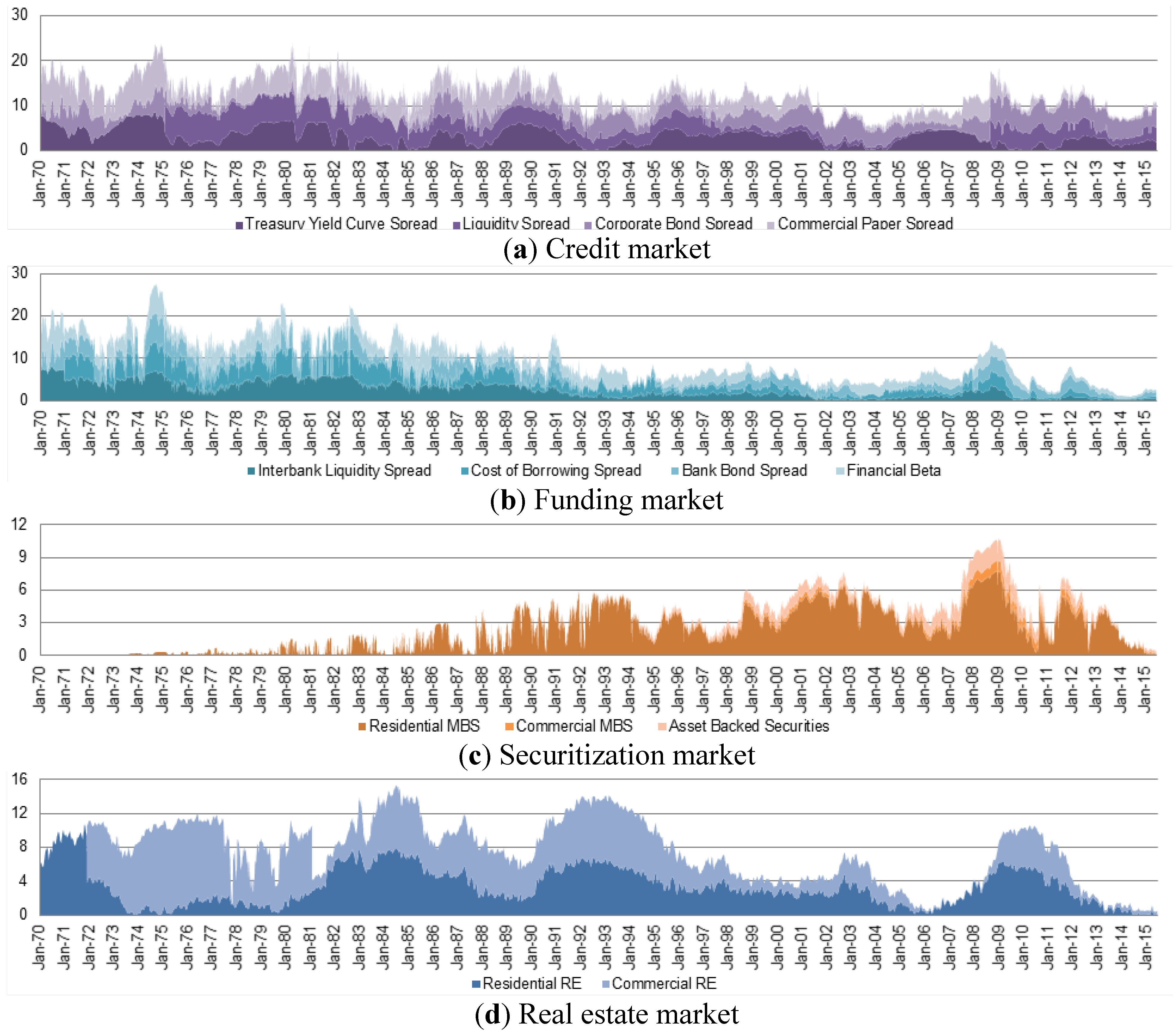
2.2.1. Financing Spread

There is rich set of theoretical precedents showing the importance of particular spreads in the context of micro- and macroeconomic equilibria. Freixas and Rochet [34] discuss how the external finance spread amplifies interest rate movement and interacts with the financial accelerator to impact monetary policy transmission, affirmed by both theoretical and empirical studies. Bernanke and Gertler [35] consider various types of spreads empirically according to their role in the credit channel of monetary policy transmission. In the theoretical study by Bernanke and Gertler [36], the importance of financing spreads for financial fragility emerges from the perspective of investment and agency costs. Finance spreads have also been associated with “scarcity of bank capital” [37], and “adverse selection in the capital markets” [38].
We define the financing spread ( F S t ) as the difference between the yield on a security or portfolio of securities ( R t r ), and the yield offered on a risk-free security of comparable maturity ( R t r f ). Therefore, we measure the risk associated with investing in the specified representative risky portfolio following Equation (1).
F S t = R t r R t r f
This indicator is used to analyze the corporate bond and commercial paper instruments in the credit market in addition to the interbank and financial bond instruments for financial institutions’ funding. We also use the financing spread to look at risk in residential, commercial, and asset backed securitization.

2.2.2. Market Beta

Another observable stress-revealing signal is a shift in the relationship between a market’s subsector of interest and the corresponding market. This market beta ( M B t ) indicator captures strains on the profitability of the selected market component compared to overall market profitability. The M B t calculation is given by:
M B t = C o v ( P t , M t ) V a r ( M t )
where P t represents the price of a designated sub-market index, and M t is an overall market index. For this specific indicator the C o v and V a r operators calculate the covariance and variance respectively over a rolling 250 day window (approximately one year of trading days), though other window widths could be of use. We use this approach to look for deviations in profitability between the financial sector (S&P 500 Financials) and the broader equity market (S&P 500).

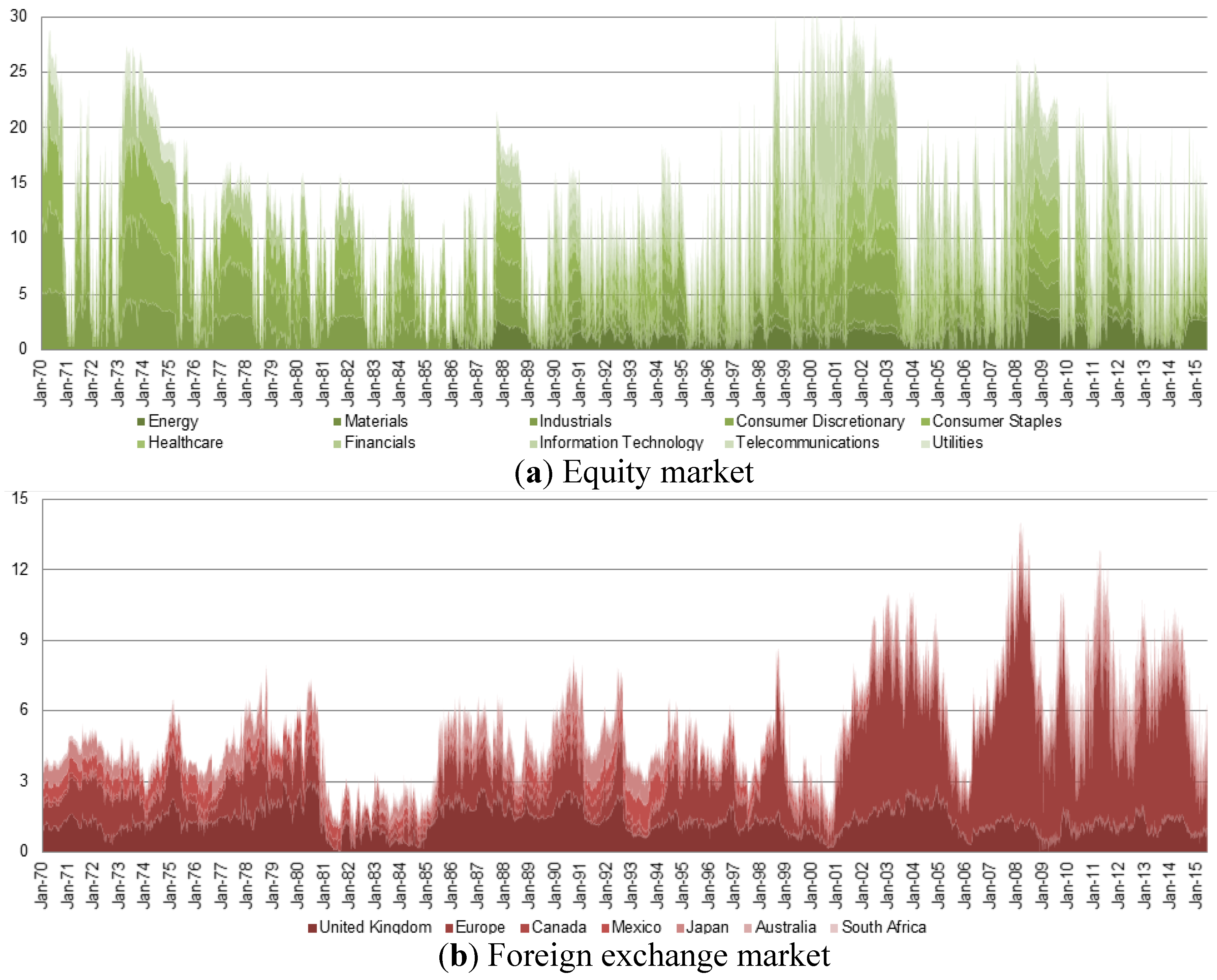
2.2.3. Market Crashes

Patel and Sarkar [39] propose a measure of recent downward movement in a specific index called the market crash. This may indicate that new information prompted a material revaluation, a cycle has caused deviations from true value, or irrational behavior is destroying value. We measure the extent of a crash in designated markets following:
M C t = P t max { P s | t 250 s t }
where P t represents the price of a designated market index, and the denominator finds the highest value in the past 250 trading days. We apply this measure to sectors of the stock market (following the GICS decomposition of the S&P 500). Similarly, depreciation of the domestic currency may indicate a set of policies or conditions which reduce demand for that currency, interpreted as stress. This foreign exchange exposure is analyzed for seven of the G20 economies which have floating exchange rates, and large trade balances with the US.

2.2.4. Covered Interest Spread

The covered interest spread ( C I S ) measures foreign exchange market inefficiency [40]. For instance, disruptions in short term US funding instruments, high demand for funding in US Dollars, and constrained capital created a persistent deviation from interest rate parity during the recent financial crisis [41]. Baba and Packer [42] find that creditworthiness of financial institutions of the US and Europe was negatively related to C I S . Using government bill yields ( R B ) from foreign nation B as the counterpart to yields on bills from domestic nation A ( R A ), the law of no arbitrage in efficiently functioning government-debt markets should drive the covered interest spread to zero. If the spread remains persistently non-zero then C I S captures the risk-free excess return that arbitrageurs could earn [40]. The calculation is:
C I S t = ( F t A B S t A B ) ( 1 + R t B ) ( 1 + R t A )
where F t A B and S t A B are the spot and forward prices respectively of one unit of currency B in terms of currency A at time t. The maturities of R t A , R t B , and F t A B should match. We calculate the C I S for seven of the G20 economies.

2.2.5. Liquidity Spread

Another measure of stress in a market is the spread between ask price ( A P t ) and bid price ( B P t ) as a component of transaction costs and the liquidity of representative instruments [43,44]. Moreover, ([45], p. 63) states that “the belief that transactions can be settled at current prices without any notable delays or transaction costs, may be a serious threat to financial stability.” As the spread (transaction cost) decreases, the security becomes more liquid which is interpreted as lower stress. We measure the short term trend in the bid-ask spread [46] as the 30 trading day moving average of the relative bid-ask spread:
L S t = ( 1 30 ) i = 0 29 [ A P t i B P t i ( A P t i + B P t i 2 ) ]
We apply this liquidity spread approach to measure liquidity in interbank instrument as an indicator for the funding market. Due to limited availability of interbank bid and ask yields we use the Eurodollar deposit bid and ask rates as a proxy [47].

2.2.6. Yield Curve Spread

The literature on the slope of the yield curve shows that this variable is a useful predictor of recessions (see [48,49,50,51]) which we expect will negatively impact credit availability. Moreover, [52] relate flattening of the yield curve to reduced profitability of existing credit portfolios. We consider the 30-day moving average of the difference between the yields offered on comparable security portfolios with long ( R t L ) and short ( R t S ) terms as follows:
Y C S t = ( 1 30 ) i = 0 29 ( R t i L R t i S )

2.2.7. Return Spread

The financing spread is forward-looking in that it incorporates the yields on risky and risk-free reference security portfolios under the assumption that the portfolio is held to maturity. From these yields we can infer information about the rate of return investors expect to earn and the perceived risk of investing in the security. However, knowledge of the expected return is not always conveniently available. Specifically, for several instrument classes only a relevant price index is available. In this case we suggest that monitors consider the spread between a realized rate of return and the risk-free yield over a holding period relevant to the underlying market.
While the market crash indicator ( M C t ) is useful for analyzing price index series it does exhibit some deficiencies. For slow moving, low volatility instruments with a positive drift term, the market crashes indicator almost identically equals unity which does not make it a suitably sensitive approach. Moreover, for some instruments we may want to take into account the potentially material influence of the risk-free rate on the net realized return. Therefore, we suggest that monitors consider the spread between a realized rate of return and the risk-free yield over a holding period relevant to the underlying market.3
R S t = ( ( P t P t M ) 1 M 1 ) R t M r f
The return spread is used for instruments where we assume a longer holding period M and incorporate the material impact of the risk-free rate with maturity M over that holding period. We calculate the return spread on residential and commercial property price indices to measure stress in the real estate market.

2.3. Indicator Transformation

Once the indicators have been prepared according to the outlined definitions above, they still possess a variety of distributions. This makes developing an aggregation scheme that preserves the interpretation of each indicator difficult. Therefore, it is useful to transform every indicator to ensure compatibility before aggregation, subject to several considerations.
The first characteristic desired for joint consideration of the stress indicators is the property that all transformed variables have compatible measures of central tendency and dispersion. Moreover, we would like the transformation to be monotonic to preserve the ordering of individual observations against the entire series. We consider two potential transformation functions satisfying these features.
The first standardization function is typically used to transform the distributions of variables from the assumed normal to the desired standard normal distribution (z-score transformation). This is achieved by shifting the central tendency measure (mean) and adjusting the dispersion (variance) following Equation (8). In the case of normal data we can use Z ( x i t ) to find the probability of an outcome less than or equal to the value of interest.
Z ( x i t ) = x i t μ i σ i
The second standardization function we consider attempts to capture the information available in a cumulative density function (CDF) empirically. This transformation shifts the mean to achieve a common measure of central tendency. The CDF transformation also modifies the range and variance to achieve a common measure of dispersion. Specifically, we calculate the CDF transform as the rank of each observation divided by the cardinality of series i ( | x i t | ) given by Equation (9) similar to [53].4 Tied observations are set as the mean of the ranks that would otherwise have been assigned. Output from the CDF transformation can be interpreted as the sample quantile such that if C D F ( x i t ) = 90 then x i t is greater than 90% of observations [54,55]. Note that the maximum C D F ( x i t ) possible of 100 is interpreted as “maximum stress observed” not “maximum stress possible”.
C D F ( x i t ) = 100 R a n k ( x i t ) | x i t |
Each of these transformations can be applied using one of two dataset partitions: (1) using the entire dataset (full information approach), (2) using all data up until time t (cumulative approach). The full information approach re-assesses every observation when a single new data value becomes available. This is unsuitable for constructing a forecasting model where we would like to easily conduct in-sample and out-of-sample testing. However, under the assumption that indicators measure time invariant relationships, leveraging the most data available also provides the truest assessment of stress. The cumulative perspective uses the information available at time t to standardize observation x i t and therefore provides a measure of stress as it would have been perceived by observers at time t . These two approaches converge as t increases, since the respective dataset partitions become increasingly similar. We confirm the observation of [56] that the difference in aggregate stress produced by these approaches is relatively minor. Therefore, we will use the full information approach in the remainder of this paper to provide the most accurate assessment and comparison of stress over time.
The CDF transformation fixes the skewness and kurtosis in the process of standardizing the range which limits the prudential ability to interpret the severity of extreme stress.5 Nevertheless, we choose to use the CDF transform due to two comparative advantages. First, the quantile focused interpretation of the CDF transformation makes no assumptions about the distribution of indicator series. In contrast, the ability to calculate P   ( x < x i t ) using the z-score relies upon the normality of x i t which is not appropriate for our indicators as shown in Table 2. Second, an average aggregate stress level of zero using the z-score may be mistakenly interpreted as nonexistent stress by an unwary observer. The CDF transformation will produce an expected stress level of 50 in addition to a positive and bounded range ( C D F ( x i t ) ( 0 , 100 ] ) which helps avoid potential misinterpretations.
Table 2. Descriptive statistics and normality testing for raw stress indicators.
NameNMinimumMaximumMeanStd. DeviationSkewnessKurtosisKolmogorov−Smirnov A
EQ_SP5EENE_DD76900.461.000.920.09−2.15 (0.03)5.72 (0.06)0.18 ***
EQ_SP5EMAT_DD67320.381.000.910.10−2.18 (0.03)5.79 (0.06)0.19 ***
EQ_SP5EIND_DD118570.381.000.920.10−1.9 (0.02)3.96 (0.04)0.2 ***
EQ_SP5ECOD_DD118570.471.000.920.09−1.64 (0.02)2.74 (0.04)0.19* **
EQ_SP5ECST_DD118570.541.000.930.07−1.66 (0.02)2.96 (0.04)0.19 ***
EQ_SP5EHCR_DD74250.621.000.930.08−1.14 (0.03)0.38 (0.06)0.17 ***
EQ_SP5EFIN_DD118570.221.000.900.12−2.17 (0.02)6.05 (0.04)0.19 ***
EQ_SP5EINT_DD76900.331.000.890.14−1.81 (0.03)2.86 (0.06)0.2 ***
EQ_SP5ETEL_DD67320.411.000.890.12−1.52 (0.03)1.75 (0.06)0.17 ***
EQ_SP5EUTL_DD118570.471.000.920.09−1.94 (0.02)3.56 (0.04)0.19 ***
FX_GBP_DD118570.671.000.930.07−1.28 (0.02)1.14 (0.04)0.14 ***
FX_EUR_DD118570.681.000.920.06−0.79 (0.02)−0.11 (0.04)0.12 ***
FX_ZAR_DD118570.511.000.890.09−0.86 (0.02)0.44 (0.04)0.12 ***
FX_CAD_DD118570.711.000.960.04−1.84 (0.02)5.79 (0.04)0.13 ***
FX_AUD_DD118570.631.000.930.06−1.27 (0.02)1.87 (0.04)0.15 ***
FX_MXN_DD118570.151.000.860.18−1.68 (0.02)1.98 (0.04)0.23 ***
FX_JPY_DD118570.751.000.930.06−0.91 (0.02)0.04 (0.04)0.13 ***
FX_GBP_CIS11857−0.040.080.020.020.66 (0.02)0.15 (0.04)0.1 ***
FX_CAD_CIS11857−0.020.060.010.010.4 (0.02)−0.08 (0.04)0.07 ***
FX_EUR_CIS4302−0.020.050.000.010.3 (0.04)0.4 (0.07)0.04 ***
FX_MXN_CIS4826−0.020.300.050.042.21 (0.04)5.83 (0.07)0.23 ***
FX_ZAR_CIS8276−0.020.140.050.02−0.2 (0.03)0.63 (0.05)0.04 ***
FX_JPY_CIS8276−0.070.04−0.010.02−0.07 (0.03)−1.01 (0.05)0.07 ***
FX_AUD_CIS7968−0.030.110.030.020.96 (0.03)0.5 (0.05)0.11 ***
CR_CBS11857−0.010.030.010.010.20 (0.02)-0.06 (0.04)0.06 ***
CR_CPS118570.000.050.010.012.6 (0.02)9.87 (0.04)0.18 ***
CR_LIQS_MA105350.000.000.000.001.78 (0.02)3.76 (0.05)0.24 ***
CR_TYC_MA11857−0.030.050.020.01−0.61 (0.02)−0.1 (0.04)0.07 ***
IB_LS118570.000.070.010.011.89 (0.02)4.46 (0.04)0.16 ***
IB_CS11603−0.050.070.010.011.61 (0.02)9.17 (0.05)0.2 ***
IB_BBS11857−0.010.070.010.012.95 (0.02)14.06 (0.04)0.14 ***
IB_FB11857−0.160.690.290.130.15 (0.02)0.21 (0.04)0.02 ***
RE_RRE11857−0.130.12−0.010.050.06 (0.02)−0.92 (0.04)0.04 ***
RE_CRE11357−0.580.15−0.020.14−2.15 (0.02)4.81 (0.05)0.17 ***
SEC_CMBS5848−0.010.150.010.023.66 (0.03)15.89 (0.06)0.23 ***
SEC_RMBS11857−0.010.040.010.000.38 (0.02)2.19 (0.05)0.05 ***
SEC_ABS6392−0.010.090.010.013.78 (0.03)17.19 (0.06)0.24 ***
Note: The standard deviation of skewness and kurtosis estimates is provided in parentheses. A The Lilliefors significance correction was used.

2.4. Aggregating Financial System Stress

Having selected and prepared appropriate indicators, we seek to aggregate them into a single measure of financial stress. The delicate issue in aggregation is determining how material each indicator and market is to the financial system. This study advances a systematic comparison of four alternative weighting schemes: (1) equal market weights, (2) credit weights, (3) portfolio theoretic weights, and (4) principal component weights. Each weighting methodology will determine the weight w j t assigned to indicator x j t at time t, following the continuous financial stress index (FSI) methodology of [32,57]:
F S I t =   j w j t C D F ( x j t )
In the absence of a priori knowledge of each indicator’s importance in the aggregate index, a common weighting scheme gives each of the n t indicators available at time t equal importance following Equation (11). When the z-score is used for standardization this approach is typically called “variance-equal” weights [32], provided in Equation (12). However, the equal-weighting scheme has no economic significance. The researcher also assigns more importance to financial system segments which have more indicators. As a result, we consider an alternative scheme to assign each of the n I markets an equal weight and then divide that weight evenly among the n J i , t indicators describing different perspectives of the market at time t in Equation (13). This weighting approach resolves the issue of assigning more importance to markets with more indicators. However, this scheme provides no intrinsic support for the claim that the selected markets are identically material to the financial system.
F S I t =   1 n t j = 1 n t C D F ( x j t )
F S I t =   1 n t j = 1 n t Z ( x j t )
F S I t =   i I 1 n I j J i 1 n J i , t C D F ( x j t )
The credit weighting approach has been proposed [32] as a stronger basis for economic significance. The financial system is partitioned into several markets i I   and submarkets j J i which are weighted according to the wealth they manage at the market level ( M i t ) and within the market ( V j t ) over time in Equations (14–16). When several indicators describe different perspectives of a single market or when information on the allocation of wealth within a market V i t is unavailable, we assign equal weight to each indicator’s perspective.
F S I t =   i I w i t j J i w j t C D F ( x j t )
w i t = M i t i M i t
w j t = V j t j J i V j t
Hollo et al. [56], propose the portfolio theoretic adjustment to a designated aggregation methodology which incorporates the exponentially weighted correlation between market level stress indices. We apply the portfolio theoretic approach as a modification of credit weights in Equations (17) and (18) where w t is the n I × 1 vector of market weights w i t , s t is the n I × 1 vector of market level stress s i t , and C t is the n I × n I matrix of exponentially weighted rolling cross-correlations such that C i j t is the correlation between s i t and s j t .
F S I t = ( w t s t ) C t ( w t s t )
s i t = j J i w j t C D F ( x j t )
Each of the above weighting approaches depends upon the definition of individual markets. An alternative approach which does not depend upon a potentially subjective partitioning of the system is to employ dimension reduction techniques to parse out the primary distinct factors from the financial system dataset. We therefore apply principal component analysis (PCA) to the set of transformed series C D F ( x j t ) . This approach produces orthogonal eigenvectors of the variance-covariance matrix which recognize and intentionally incorporate the structural relationships inherent in the dataset. Each of these i I eigenvectors, called factors, represents a linear combination with weights w j of several variables j J i and consolidates a particular facet of the data. We weight each factor i according to the percent of variation w i it explains in Equations (19) and (20) where l j i is the standardized loading of C D F ( x j t ) onto factor i . It is possible for the variation in a large dataset to be suitably described by a small collection of factors. We use enough factors to capture ~70 percent of the dataset’s variation [58].
F S I t =   i I w i j J i w j C D F ( x j t )
w i = j j i l j i 2 i I j J i l j i 2
The weight assigned to each factor is static which implicitly assumes that the importance of each market and the relationships between factors remains constant for all observations. This is difficult to justify in the complex and evolving financial system. Dynamic approaches to dimension reduction exist which can mitigate this concern and have been implemented by [59]. However, this is left as a topic for further study.

3. CFSI Calibration

To evaluate the candidate weighting schemes we follow the work of Oet et al. [60] which develops a framework to evaluate the information value of measures describing the state of the US financial system. They suggest comparing each FSI against a benchmark of financial system crisis using the Type I error, Type II error, noise to signal ratio ( N T S R ), information value ( I V ), and relative usefulness ( U R ( μ ) ) metrics. The Type I (Type II) error is the proportion of crisis (resp. non-crisis) events falsely classified by the candidate stress measure. The noise to signal ratio attempts to balance the Type I and Type II errors and Kaminsky et al. [61] state that a N T S R i less than one indicates a beneficial FSI. The I V metric looks for consistent association across time between the candidate FSI and the benchmark. Siddiqi [62] provides a heuristic guide that an I V less than 0.1 is weak, I V between 0.1 and 0.3 is average, I V between 0.3 and 0.5 is strong, and I V greater than 0.5 may be suspiciously high. Finally, the U R ( μ ) metric accounts for the proportion of costs μ incurred when policy is not implemented and a crisis occurs. U R ( μ ) has a desired maximum value of one reflecting a perfect alignment between FSI and benchmark. Collectively these metrics provide different insight into the nature of association between benchmark and FSI for robust analysis.
We propose in Section 2.2 that stress can be measured through spread-like indicators that capture deviations from stable relationships. While volatility series may not offer insight into the drivers of stress, they are widely used to provide a general overview of market conditions. Oet et al. [60] construct a benchmark of stress from six volatility series representing different segments of the financial system (shown in Figure 1).6 We convert the volatility series V i t into a binary indicator of systemic crisis B t following Equations (21) and (22). Crisis is defined as K consecutive periods of stress in at least one market or concurrent stress in at least L distinct markets. In this case a market is thought to be in stress if the z-score of the volatility measure is above some threshold τ B .7
B F , t = { 1   i f   i j = 0 K 1 I ( Z ( V i , t j F ) ) > 0   o r   i I ( Z ( V i , t j F ) ) L   0   o t h e r w i s e  
I ( x ) = { 1   i f   x > τ B   0   o t h e r w i s e
Figure 1. Standardized volatility series and the resulting crisis benchmark.
Risks 03 00420 g001
This definition of crisis applies a uniform standard across markets dependent upon the discriminant threshold τ B , the persistence requirement K , and the resonance requirement L . The discriminant threshold can be set somewhat low since the persistence and resonance requirements limit the opportunity for idiosyncratic events to be classified as a systemic crisis. The work of Laeven and Valencia [63] focuses on identifying banking crises and may therefore miss broader financial system crises. Indeed, they find only two crises, the first in 1988 and the second starting in 2007, which is not sufficiently granular for evaluating our financial stress indices.8
We prepare candidate FSIs for comparison against the binary crisis benchmark at a variety of frequencies F { d a i l y ,   w e e k l y ,   m o n t h l y ,   q u a r t e r l y } by taking the periodic average. Figure 2 displays the four standardized candidate stress measures at daily frequency. Then the stress index generates a signal of crisis when its z-score is greater than τ :9
S F , t = { 1   i f   Z ( F S I F , t ) > τ   0   o t h e r w i s e  
We examine the results across frequencies to support the selection of a weighting methodology in Table 3. Each of the proposed aggregation schemes produces an attractive relative usefulness U R ( μ ) near or above 0.5 and noise to signal ratio under 0.3. Although market weights exhibit superiority at monthly frequency, the approach generally produces a lower relative usefulness. Weights based upon principal component analysis and credit weights are identical at quarterly frequency and roughly equivalent otherwise. Principal component analysis weights consistently achieve a modestly lower noise to signal ratio while credit weights possess marginally superior information value across frequencies. While both of these options are comparable, credit weights are dynamic and more interpretable than their static PCA counterpart. Therefore, for the remainder of this paper we focus on exploring the functionality and interpretation of CFSI which adopts a credit weights methodology.
Figure 2. Standardized stress series under the four proposed weighting schemes.
Risks 03 00420 g002
Table 3. Comparison of information quality of alternative aggregation methods.
Name τ F , i l e v TPFPTNFNT1T2IVNTSRµ U A ( μ ) U R ( μ )
Panel 1: Quarterly ( τ B , Q l e v = 1 and 3 bins were used for IV)
1Credit Weights1.011227260.330.030.330.040.80.10.64
2Principal Component Weights1.041237160.330.040.180.060.80.10.63
3Equal Market Weights0.5613116350.280.151.080.210.80.090.57
4Portfolio Theoretic Weights0.59966890.50.080.490.160.80.070.42
Panel 2: Monthly ( τ B , M l e v = 1 and 3 bins were used for IV)
1Equal Market Weights0.683623202170.320.10.620.150.80.090.57
2Principal Component Weights0.983314211200.380.060.270.10.80.080.56
3Credit Weights0.783322203200.380.10.710.160.80.080.52
4Portfolio Theoretic Weights1.03207218330.620.030.160.080.80.050.34
Panel 3: Weekly ( τ B , W l e v = 1.2 and 4 bins were used for IV)
1Principal Component Weights0.8816395854960.370.10.520.160.80.080.5
2Credit Weights0.77154938561050.410.10.660.160.80.070.46
3Equal Market Weights0.651531138361060.410.120.750.20.80.070.43
4Portfolio Theoretic Weights0.62105668831540.590.070.220.170.70.040.3
Panel 4: Daily ( τ B , D l e v = 1.2 and 4 bins were used for IV)
1Principal Component Weights0.86120760158727810.390.090.380.150.70.080.48
2Credit Weights0.73117466158128140.410.10.620.170.70.070.45
3Equal Market Weights0.64113276157128560.430.120.60.210.70.070.41
4Portfolio Theoretic Weights0.65744401607212440.630.060.150.170.70.050.29
Although the methodologies authors employ to construct FSIs vary, we have attempted to construct a measure which aligns as closely as possible with the definitions of stress as pressure affecting each element of the financial system. As a result we have leveraged spread-like measures that focus on individual relationships which should remain stable over time, interpreting deviations as manifest stress. Other FSIs typically introduce volatility measures which offer less intuition about the specific causes of stress or potential remedial action. Aside from providing a methodology for determining the quality of information provided by a financial stress measure, [60] compare a collection of US FSIs. They find that while most measures considered possess attractive noise to signal ratios, CFSI broadly outperformed alternative stress measures in terms of relative usefulness across all frequencies.

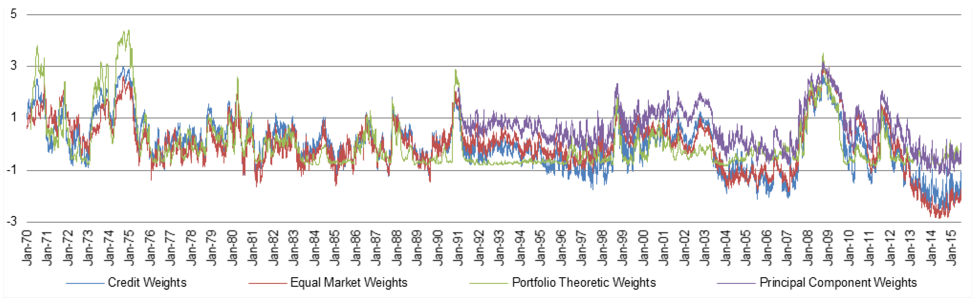
4. CFSI Interpretation

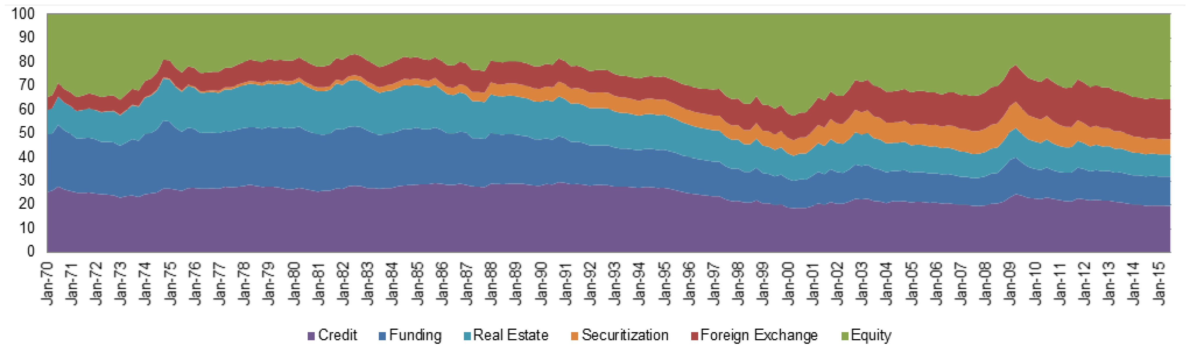
4.1. Decomposition of Stress

Potential characteristics of complex systems exhibited by financial systems are hierarchical composition and decomposability [64]. A stress measure should contribute towards critical and transparent observation of the financial system and its components. Therefore, the FSI’s ability to investigate and classify the components of system stress is particularly critical to risk managers.

4.1.1. Credit Weights

We begin by analyzing the weight attributed to each market in Figure 3. At the beginning of our time series the credit and funding markets were dominant forces with approximately 25% of the systems funds each, surpassed only by the equity market. This allocation remained fairly stable through 1995 disturbed only by steady securitization market growth. Between 1995 and the 1Q 2000 the equity market grew at an accelerated rate only to lose most of this growth by Q4 2002. The recent financial crisis again led to a decreased allocation in equity reaching a local minimum in Q1 2009, followed by a relatively rapid expansion of the equity market through Q1 2015. The securitization market, although smaller, acquired a steadily expanding place in the financial system through Q1 2009, at which point it began to wane. Interestingly, the share of the financial system associated with the foreign exchange market has grown steadily since 1970 potentially reflecting increased globalization of the financial sector.
Figure 3. Decomposition of the weight attributed to designated financial system markets.
Risks 03 00420 g003
Having briefly considered changes over time in financial system composition we shift our focus to financial system stress as described in Figure 4 which contains CFSI at a daily frequency. Cursory inspection reveals periods of persistent elevated stress in several markets. Between Q1 1973 and Q2 1975 the equity, funding, and credit markets experienced stress which would not be repeated until the recent financial crisis.10 The inflationary period between Q1 1976 and Q2 1982 produced stress in the funding, credit, and real estate markets; however, a dearth of material equity stress produced a prolonged period of only moderately elevated system stress. Between 1991 and 1998, there was a period of progressive movement towards stability. This was broken abruptly by material stress in the equity markets in Q3 1998 at the time of the Long-Term Capital Management (LTCM) crisis and again between Q1 2000 and Q1 2003 with a sequence of equity market crashes (the dot-com bubble and the early 2000s recession). Between 2003 and 2007, the financial system remained relatively tranquil with extremely low stress as the real estate market experienced several years of growth while all other markets also experienced subdued stress. However, in Q2 of 2007, increased stress began to accumulate in credit, funding, and securitization markets. By Q1 of 2008, the equity and foreign exchange markets were also experiencing heightened stress which peaked in October of 2008. Stress presented itself again in Q3 2011 due to concerns over the foreign exchange, funding, and equity markets.
Figure 4. Decomposition of financial system stress among the six designated markets.
Risks 03 00420 g004

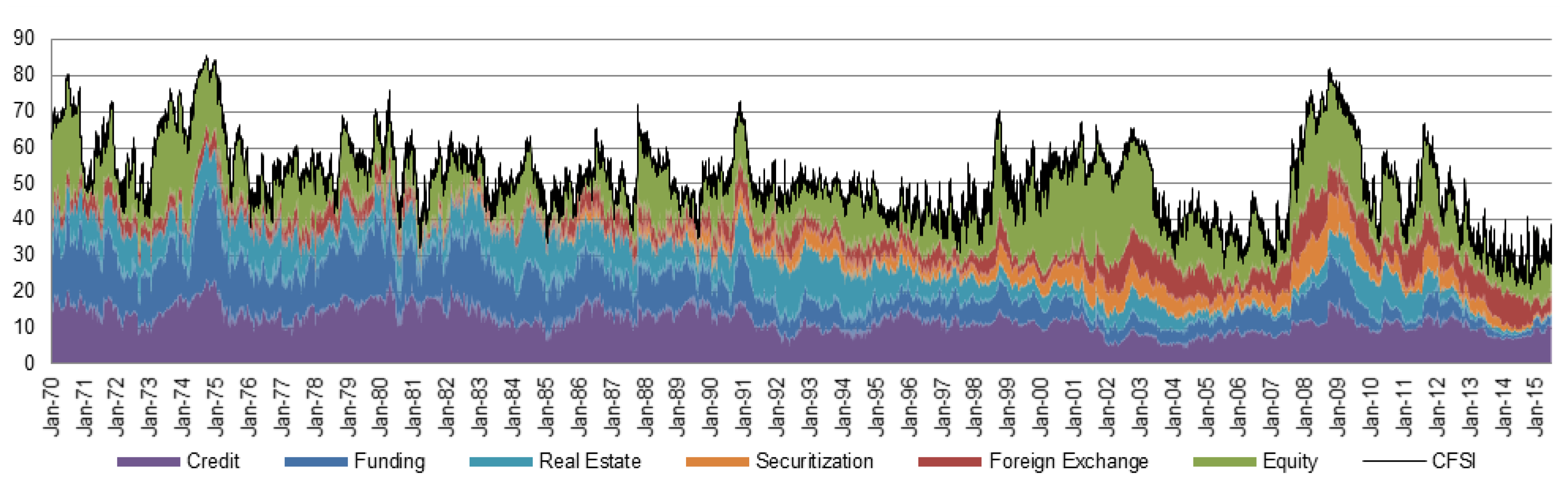
4.1.2. Market Components

The modular stress construction employed by CFSI enables informative decomposition and analysis of system stress into market components (Figure 5 and Figure 6). In Figure 5(a,b) we describe the credit and funding markets, respectively. Generally speaking, between 1970 and 1991 both of these markets experienced a fair amount of stress, followed in 1993 through early 2007 by a period of relative tranquility before the financial crisis. However, the pattern of component stress development is distinct to each market. For instance, in 2006 leading up to the financial crisis the treasury yield curve spread approached its maximum while the corporate bond and commercial paper spreads hovered at average levels, and the liquidity spread indicated low liquidity pressure. It is not until the first half of 2008 that liquidity begins to dry up, while the corporate bond and commercial paper spreads widen. These three concurrent trends produce a noticeable rise in overall credit market stress. In Figure 5(c,d) we focus on the components of the securitization and real estate markets, respectively. The securitization market contributes a steadily increasing amount of stress through 2003, as the market grows to occupy a more material position in the financial system. The decomposition of securitization components from 2004 through late 2007 reveals relatively low risk valuations in the market. Between 2007 and 2010, the market spreads on these instruments are reassessed at a higher risk level producing a material increase in securitization market stress. The decrease in securitization market stress since Q2 2011 is due to (1) a steady reduction in the relative size of this market (Figure 3) and (2) a return towards lower risk being priced into securitized products. Care must be taken in reading these graphs of market stress, since they are the combination of standardized stress indicators and changing market weights. Therefore, as we have just illustrated for the securitization market, movement in the market’s stress may be attributable to either a change in the market’s significance or to indicator movement. This insight is reaffirmed in interpreting the real estate market from Figure 5d. Observers should recognize that the real estate market’s weight has decreased, instead of interpreting real estate market stress in 2007 as less extreme than stress witnessed in 1984 or 1992.
Figure 5. Financial stress in the credit (a); funding (b); securitization (c); and real estate (d) markets in terms of their constituent indicators.
Risks 03 00420 g005
Figure 6. Financial stress in the equity (a) and foreign exchange (b) markets in terms of their constituent indicators.
Risks 03 00420 g006
Figure 6 examines the equity and foreign exchange markets in detail. Between 1970 and 1994, crises in the equity market (panel a) appear to impact the various equity sub-markets uniformly, after accounting for the relative size of each market and the growing number of sub-markets considered.11 However, beginning in 1998 equity market stress becomes more localized in specific affected sectors. The 1998 LTCM crisis focused on the financial sector. Beginning in Q2 2000, several sectors experienced difficulty together with the information technology sector. In Q1 2001 the financial and healthcare sectors began to drop, followed in Q3 2001 by modest stress increases in the consumer discretionary and industrial sectors. The decomposition of stress in the foreign exchange market (panel b) shows that over time, contributions to US stress emanate mainly from exposures to Europe and the United Kingdom.12 Nevertheless, market stress components confirm the historical evidence of upheavals due to other countries, such as the 1993 exposure to Mexico or concerns over Japan between 1990 and 1992.13

4.2. Historical Relevance of Stress

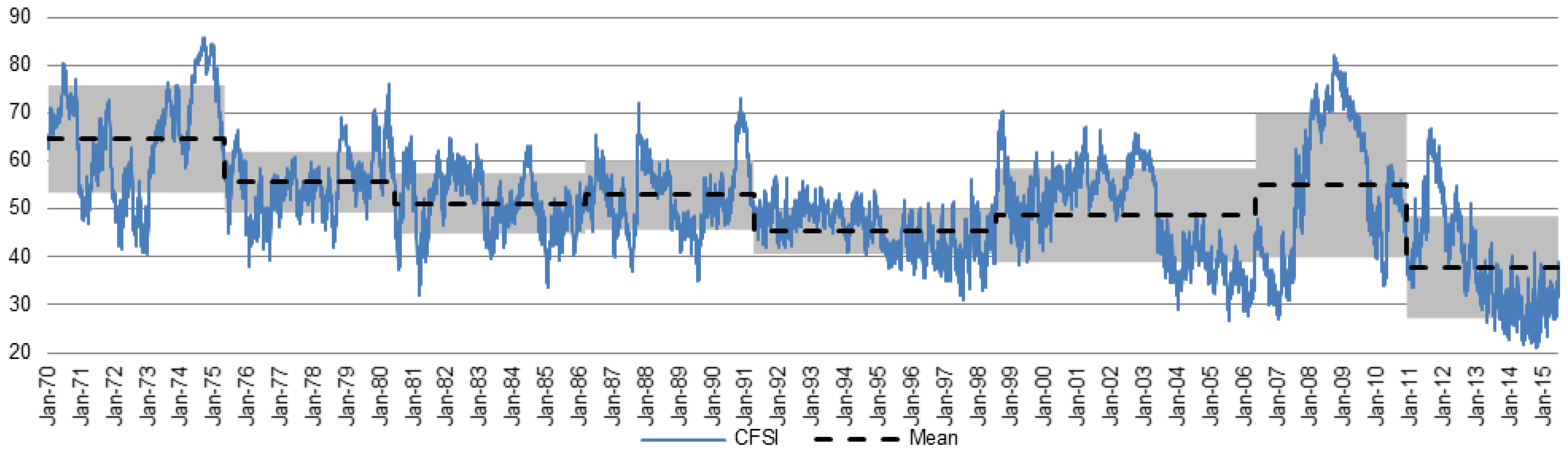
4.2.1. Stress Regimes

In this section, we present evidence of structural transformations in financial system stress. We apply a sequential approach to determine the presence and location of structural breaks in the level of stress. We allow for breaks in the dispersion of stress (error distribution) across time following [65]. The minimum allowable region length is set as h = t r × T , where t r = 10 % is the trim parameter and T is the total number of observations, to avoid estimating a model based upon insufficient data. The results presented in Table 4 indicate the presence of seven structural breaks which are significant at 1%.
Table 4. Results for the Bai-Perron sequential test for structural breaks.
Break TestScaled F-StatisticCritical Value ***ABreak Date
0 vs. 1 ***2773.1913.0006/24/1980
1 vs. 2 ***1368.5314.5112/07/2010
2 vs. 3 ***669.8615.4405/09/1975
3 vs. 4 ***166.9215.7305/23/2006
4 vs. 5 ***736.4216.3904/11/1991
5 vs. 6 ***184.0916.6007/23/1998
6 vs. 7 ***47.1216.7803/19/1986
7 vs. 80.0016.90not found
Note: *** indicates significance at 1%. A Critical values are calculated following [66].
Figure 7. Daily CFSI compared to the mean and standard deviation (shaded region) of stress in each sub-period.
Risks 03 00420 g007
Clearly the early 1970s experienced a period of heightened stress in several markets leading to the structural break of 1975 when the average level of stress shifted to a lower level regime (see Figure 7). The structural break in 1980 coincides with the return towards historic inflation rates starting in Q2 1980 from the heightened inflation between 1973 and 1982. Fed by an accommodating regulatory environment (deregulation and forbearance), the US savings and loan (S&L) institutions experienced substantial growth between 1982 and 1985 [67]. However, difficulties due to recent inflation, in turn, led to a protracted string of material defaults between 1982 and 1993 [52]. Even with residual distress from the S&L crisis and exposure to Mexican and Japanese distress between 1991 and 1993, the period spanning 1991 through 1998 exhibits below average stress and a reduced variance in stress as the US economy prospers. In contrast, the LTCM crisis in 1998 and the successive equity market declines between 2000 and 2003 produce a regime of heightened volatility. The 2006 structural break denotes a regime of the highest volatility among recorded time partitions and is accentuated with the high 2008 financial crisis levels of stress not seen since 1975. Finally, the post-2010 regime is characterized by an average level of stress that is lower than all observed historical periods with historically standard volatility.

4.2.2. Links to Regulation

There is a strong empirical link between regulation and systemic crises. Miron [68] concludes that prior to the creation of the Federal Reserve, banking panics in the United States were seasonal. Similarly, Kemmerer [69] states that between 1890 and 1908, there were 28 US banking panics. Freixas and Rochet [34] find that many financial crises worldwide have been partly initiated by a global movement toward financial deregulation. Mishkin emphasizes this point in discussing the US savings and loan crisis, asserting that “deregulation of a financial system and rapid credit growth can be disastrous if banking institutions and their regulators do not have sufficient expertise to keep risk taking in check” [17] (p. 28). In an extensive empirical review of US bank deregulation, Calomiris states that, “the single most important factor in banking instability has been the organization of the banking industry” [70] (p. 3).
The US Financial Services Modernization Act (the Gramm–Leach–Bliley Act) became law in 1999, demolishing the structural separation that formerly existed between commercial banks, investment banks, securities firms, and insurance companies. Universal banking allows financial intermediaries to grow larger and more diverse, enabling them to benefit from more efficient portfolio diversification to take larger risk.14 However, allowing banks to diversify may increase the similarity of banks’ portfolios thereby decreasing the system’s diversification and increasing systemic risk. Once crisis sets in, contagion among institutions due to correlated exposures can be expected to persist longer.
Figure 8. Fraction of systemic stress episodes with the given durations (measured in weeks) for selected severity (a) τ = 0.5 , (b) τ = 1.25 .
Risks 03 00420 g008
Analyzing the length of consecutive stress episodes generated when the standardized weekly CFSI is above τ provides limited support for the influence of financial regulation on systemic crises (Figure 8). We observe that after deregulation, the length of low severity ( τ = 0.5 ) and moderate severity ( τ = 1.25 ) crises following Equation (23) becomes modestly more polarized. After 1998 crises tend to resolve more quickly—the benefit of diversified institutions (Figure 8a). However, the high severity episodes tend to last somewhat longer reflecting a heightened system exposure to material events (Figure 8b). Meanwhile, the percentage of observations experiencing a crisis is slightly higher before 1998 at 12.05% than after 1998 at 9.76% (for τ = 1.25 ).

5. Conclusions

The construction of CFSI described in this paper illustrates a systematic approach to constructing and calibrating a measure of financial system stress. This paper carefully explores the motivation and support for each indicator while expanding coverage of the equity and foreign exchange markets. We consider candidate weighting methodologies that include equal market weights, credit weights, portfolio theoretic weights, and principal component analysis weights. We comprehensively explore the information quality of each index construction at various frequencies to validate the selection of credit weights. We demonstrate that CFSI is useful for decomposing stress, monitoring its development, and historical analysis. To the authors’ knowledge, this construction constitutes the deepest high-frequency measure of US financial system stress currently available for analysis.
However, the subject of stress measurement offers many additional opportunities for constructive research. While the markets considered in the construction of CFSI are doubtless material to the financial system, present analysis cannot support a claim that they comprehensively partition the financial system. This opens the door to future rigorous approaches on quantitative decomposition of the financial system in terms of financial instruments, agents, and intermediation functions. Moreover, in this paper the relative parity of information quality between principal component analysis and credit weighting schemes is broken by the improved interpretability and the dynamic nature of the credit weighing methodology. However, dynamic principal component analysis may accommodate the adaptive nature of the financial system through non-constant weights and avoid the critique of arbitrary market selection suffered by credit weights making it an attractive candidate for further study.

Acknowledgments

The authors would like to thank Joseph Haubrich, Ben Craig, and Mark Schweitzer for constructive guidance and formative suggestions. We are grateful to James Thomson, Mark Sniderman, Viral Acharya, John Schindler, Myong-Hun Chang, Manfred Kremer, Marco Lo Duca, Tuomas Peltonen, and Mark Flood for valuable comments. The authors thank the participants of the 2014 International work-conference on Time Series, the 2014 IRMC conference on “The Safety of the Financial System—From Idiosyncratic to Systemic Risk”, the 6th International IFABS Conference on “Alternative Futures for Global Banking: Competition, Regulation and Reform”, the 12th INFINITI conference on international finance, the 2010 Deutsche Bundesbank/Technische Universitat Dresden conference, “Beyond the Financial Crisis,” the 2010 Federal Regulatory Interagency Risk Quantification Forum, the 2010 Federal Reserve Committee on Financial Structure and Regulation, the Federal Reserve Bank of Chicago 2009 Capital Markets Conference, and the 2009 NBER—Federal Reserve Bank of Cleveland’s Research Conference on Quantifying Systemic Risk for helpful comments and suggestions. In addition, we wish to thank Tim Bianco, Amanda Janosko, Ryan Eiben, and Dieter Gramlich for instrumental critiques and research assistance.

Author Contributions

All authors contributed materially to conceptual development of the paper and writing.

Conflicts of Interest

The authors declare no conflict of interest.

References

  1. G. Caprio, and D. Klingebiel. Bank Insolvencies: Cross Country Experiences. World Bank Policy Research Working Paper No. 1620; Washington, DC, USA: The Work Bank, 1996. [Google Scholar]
  2. A. Demirgüç-Kunt, and E. Detragiache. “The determinants of banking crises in developing and developed countries.” IMF Staff Pap. 45 (1998): 81–109. [Google Scholar] [CrossRef]
  3. O. De Bandt, and P. Hartmann. Systemic risk: A Survey. European Central Bank Working Paper No. 35; Frankfurt, Germany: European Central Bank, 2000. [Google Scholar]
  4. Y. Ishihara. Quantitative Analysis of Crisis: Crisis Identification and Causality. World Bank Policy Research Working Paper No. 3598; Washington, DC, USA: The Work Bank, 2005. [Google Scholar]
  5. E.P. Davis, and D. Karim. “Comparing early warning systems for banking crises.” J. Financ. Stab. 4 (2008): 89–120. [Google Scholar] [CrossRef]
  6. M.D. Bordo, M. Dueker, and D. Wheelock. Aggregate Price Shocks and Financial Instability: An Historical Analysis. Federal Reserve Bank of St. Louis Working Paper No. 005B; St. Louis, MO, USA: Federal Reserve Bank of St. Louis, 2000. [Google Scholar]
  7. M. Rosenberg. “Financial Conditions Watch, Global Financial Market Trends and Policy. Bloomberg LLP.” Available online: http://www.ssc.wisc.edu/~mchinn/fcw_sep112009.pdf (accessed on 1 July 2015).
  8. W. English, K. Tsatsaronis, and E. Zoli. “Assessing the predictive power of measures of financial conditions for macroeconomic variables.” In Investigating the Relationship between the Financial and Real Economy. BIS Paper No. 22; Basel, Switzerland: Bank for International Settlements (BIS), 2005, pp. 228–252. [Google Scholar]
  9. A. Swiston. A U.S. Financial Conditions Index. International Monetary Fund Working Paper No. 16; Washington, DC, USA: International Monetary Fund, 2008. [Google Scholar]
  10. J.B. Thomson. On Systemically Important Financial Institutions and Progressive Systemic Mitigation. FRB of Cleveland Policy Discussion Paper No. 7; Cleveland, OH, USA: FRB of Cleveland, 2007. [Google Scholar]
  11. N. Liang. “Systemic risk monitoring and financial stability.” J. Money Credit Bank. 45 (2013): 129–135. [Google Scholar] [CrossRef]
  12. E.S. Rosengren. “Defining financial stability, and some policy implications of applying the definition.” In Keynote Remarks. Stanford, CA, USA: Stanford Finance Forum Graduate School of Business, 2011. [Google Scholar]
  13. G. Schinasi. “Understanding Financial Stability: Towards a Practical Framework.” In Proceedings of the Seminar on Current Developments in Monetary and Financial Law, Washington, DC, USA, 23–27 October 2006.
  14. J. Laker. “Monitoring financial system stability.” Reserv. Bank Aust. Bull. 10 (1999): 40–46. [Google Scholar]
  15. R.W. Ferguson. “Should financial stability be an explicit central bank objective.” In Proceedings of the International Monetary Fund Conference: Monetary Stability, Financial Stability and the Business Cycle, Washington, DC, USA, 27–28 October 2003; pp. 208–223.
  16. A. Crockett. “Why is financial stability a goal of public policy? ” Fed. Reserv. Bank Kansas City Econ. Rev. 82 (1997): 5–22. [Google Scholar]
  17. F.S. Mishkin. “The causes and propagation of financial instability: Lessons for policymakers.” In Maintaining Financial Stability in a Global Economy. Kansas City, MO, USA: Federal Reserve Bank of Kansas City, 1997, pp. 55–96. [Google Scholar]
  18. J. Simmie, and R. Martin. “The economic resilience of regions: Towards an evolutionary approach.” Camb. J. Regions Econ. Soc. 3 (2010): 27–43. [Google Scholar] [CrossRef]
  19. G.L. Kaminsky, and C.M. Reinhart. “The twin crises: The causes of banking and balance-of-payments problems.” Am. Econ. Rev. 89 (1999): 473–500. [Google Scholar] [CrossRef] [Green Version]
  20. A. Demirgüç-Kunt, and E. Detragiache. Cross-Country Empirical Studies of Systemic Bank Distress: A Survey. IMF Working Paper No. 96; Washington, DC, USA: International Monetary Fund (IMF), 2005. [Google Scholar]
  21. L. Laeven, and F. Valencia. Systemic Banking Crises: A New Database. IMF Working Paper No. 224; Washington, DC, USA: International Monetary Fund (IMF), 2008. [Google Scholar]
  22. C. Reinhart, and K. Rogoff. This Time Is Different: A Panoramic View of Eight Centuries of Financial Crises. NBER Working Paper No. 13882; Cambridge, MA, USA: National Bureau of Economic Research (NBER), 2008. [Google Scholar]
  23. W.A. Brock, and C.H. Hommes. “A rational route to randomness.” Econometrica 65 (1997): 1059–1095. [Google Scholar] [CrossRef]
  24. W.A. Brock, and C.H. Hommes. “Heterogeneous beliefs and routes to chaos in a simple asset pricing model.” J. Econ. Dyn. Control 22 (1998): 1235–1274. [Google Scholar] [CrossRef]
  25. C.H. Hommes. “Financial markets as nonlinear adaptive evolutionary systems.” Quant. Financ. 1 (2001): 149–167. [Google Scholar] [CrossRef]
  26. P. Aghion, and P. Howitt. “A model of growth through creative destruction.” Econometrica 60 (1992): 323–351. [Google Scholar] [CrossRef]
  27. P. Howitt, A. Kirman, A. Leijonhufvud, P. Mehrling, and D. Colander. “Beyond DSGE models: Toward an empirically based macroeconomics.” Am. Econ. Rev. 98 (2008): 236–240. [Google Scholar]
  28. J.D. Farmer. “Market force, ecology and evolution.” Ind. Corp. Chang. 11 (2002): 895–953. [Google Scholar] [CrossRef]
  29. J.D. Farmer, P. Patelli, and I.I. Zovko. “The predictive power of zero intelligence in financial markets.” Proc. Natl. Acad. Sci. USA 102 (2005): 2254–2259. [Google Scholar] [CrossRef] [PubMed]
  30. D. Hendricks, J. Kambhu, and P. Mosser. “Systemic Risk and the Financial System.” Fed. Reserv. Bank N. Y. Econ. Policy Rev. 13 (2007): 65–80. [Google Scholar]
  31. J. Kambhu, S. Weidman, and N. Krishnan. “Introduction: New directions for understanding systemic risk.” Fed. Reserv. Bank N. Y. Econ. Policy Rev. 13 (2007): 3–14. [Google Scholar]
  32. M. Illing, and Y. Liu. “Measuring financial stress in a developed country: An application to Canada.” J. Financ. Stab. 2 (2006): 243–265. [Google Scholar] [CrossRef]
  33. D. Gramlich, G. Miller, M. Oet, and S. Ong. “Early Warning Systems for Systemic Banking Risk: Critical Review and Modeling Implications.” Bank. Bank Syst. 5 (2010): 199–211. [Google Scholar]
  34. X. Freixas, and J.-C. Rochet. Microeconomics of Banking, 2nd ed. Cambridge, MA, USA: The MIT Press, 2008. [Google Scholar]
  35. B. Bernanke, and M. Gertler. “Inside the black box: The credit channel of monetary policy transmission.” J. Econ. Perspect. 9 (1995): 27–48. [Google Scholar] [CrossRef]
  36. B.S. Bernanke, and M. Gertler. “Financial fragility and economic performance.” Q. J. Econ. 105 (1990): 97–114. [Google Scholar] [CrossRef]
  37. B. Holmström, and J. Tirole. “Financial intermediation, loanable funds, and the real sector.” Q. J. Econ. 112 (1997): 663–691. [Google Scholar] [CrossRef]
  38. P. Bolton, and X. Freixas. “Equity, bonds, and bank debt: Capital structure and financial market equilibrium under asymmetric information.” J. Political Econ. 108 (2000): 324–351. [Google Scholar] [CrossRef]
  39. S.A. Patel, and A. Sarkar. “Crises in developed and emerging stock markets.” Financ. Anal. J. 54 (1998): 50–61. [Google Scholar] [CrossRef]
  40. M.P. Taylor. “Covered interest arbitrage and market turbulence.” Econ. J. 99 (1989): 376–391. [Google Scholar] [CrossRef]
  41. T. Mancini-Griffoli, and A. Ranaldo. “Limits to arbitrage during the crisis: Funding liquidity constraints and covered interest parity.” Available online: http://papers.ssrn.com/sol3/papers.cfm?abstract_id=1569504. (accessed on 5 August 2015).
  42. N. Baba, and F. Packer. “From turmoil to crisis: Dislocations in the FX swap market before and after the failure of Lehman Brothers.” J. Int. Money Financ. 28 (2009): 1350–1374. [Google Scholar] [CrossRef]
  43. A. Crockett. “Market liquidity and financial stability.” Banq. Fr. Financ. Stab. Rev. 11 (2008): 13–17. [Google Scholar]
  44. J. Caruana, and L. Kodres. “Liquidity in global markets.” Banq. Fr. Financ. Stab. Rev. 11 (2008): 65–74. [Google Scholar]
  45. A. Bervas. “Market liquidity and its incorporation into risk management.” Banq. Fr. Financ. Stab. Rev. 8 (2006): 63–79. [Google Scholar]
  46. L. Chen, D.A. Lesmond, and J. Wei. “Corporate yield spreads and bond liquidity.” J. Financ. 62 (2007): 119–149. [Google Scholar] [CrossRef]
  47. D. Hou, and D.R. Skeie. LIBOR: Origins, Economics, Crisis, Scandal, and Reform. FRB of New York Staff Report No. 667; New York, NY, USA: FRB of New York, 2014. [Google Scholar]
  48. A. Estrella, and G. Hardouvelis. “The term structure as a predictor of real economic activity.” J. Financ. 46 (1991): 555–576. [Google Scholar] [CrossRef]
  49. A. Estrella, and F. Mishkin. “The yield curve as a predictor of U.S. recessions.” Fed. Reserv. Bank N. Y. Curr. Issues Econ. Financ. 2 (1996): 1–6. [Google Scholar] [CrossRef]
  50. J. Haubrich, and T. Bianco. The Yield Curve as a Predictor of Economic Growth. Cleveland, OH, USA: Federal Reserve Bank of Cleveland, 2011. [Google Scholar]
  51. S. Gilchrist, and E. Zakrajšek. Credit Spreads and Business Cycle Fluctuations. NBER Working Paper No. w17021; Cambridge, MA, USA: National Bureau of Economic Research (NBER), 2011. [Google Scholar]
  52. M. Goodfriend. “Financial Stability, Deflation, and Monetary Policy.” Monet. Econ. Stud. 19 (2001): 143–176. [Google Scholar] [CrossRef]
  53. A. Spanos. Probability Theory and Statistical Inference: Econometric Modeling with Observational Data. Cambridge, UK: Cambridge University Press, 1999. [Google Scholar]
  54. R. Koenker, and G. Bassett Jr. “Regression quantiles.” Econometrica 46 (1978): 33–50. [Google Scholar] [CrossRef]
  55. R. Koenker. Quantile Regression. Cambridge, UK: Cambridge University Press, 2005. [Google Scholar]
  56. D. Hollo, M. Kremer, and M. Lo Duca. CISS-A Composite Indicator of Systemic Stress in the Financial System. ECB Working Paper Series No. 1426; Frankfurt, Germany: European Central Bank (ECB), 2012. [Google Scholar]
  57. M. Illing, and Y. Liu. An Index of Financial Stress for Canada. Bank of Canada Working Paper No. 14; Ottawa, ON, Canada: Bank of Canada, 2003. [Google Scholar]
  58. J.F. Hair, W.C. Black, B.J. Babin, R.E. Anderson, and R.L. Tatham. Multivariate Data Analysis, 7th ed. Upper Saddle River, NJ, USA: Pearson Prentice Hall, 2009. [Google Scholar]
  59. S.A. Brave, and R.A. Butters. “Monitoring financial stability: A financial conditions index approach.” Econ. Perspect. 35 (2011): 22–43. [Google Scholar]
  60. M.V. Oet, J. Dooley, D. Gramlich, P. Sarlin, and S. Ong. Evaluating the Information Value for Measures of Systemic Conditions. Federal Reserve Bank of Cleveland Working Paper No. 15/13; Cleveland, OH, USA: Federal Reserve Bank of Cleveland, 2015. [Google Scholar]
  61. G. Kaminsky, S. Lizondo, and C.M. Reinhart. “Leading indicators of currency crises.” IMF Staff Pap. 45 (1998): 1–48. [Google Scholar] [CrossRef] [Green Version]
  62. N. Siddiqi. Credit Risk Scorecards: Developing and Implementing Intelligent Credit Scoring. Cary, NC, USA: SAS Institute, 2006, pp. 79–83. [Google Scholar]
  63. L. Laeven, and F. Valencia. “Systemic banking crises database.” IMF Econ. Rev. 61 (2012): 225–270. [Google Scholar] [CrossRef]
  64. H.A. Simon. “The Architecture of Complexity.” Proc. Am. Philos. Soc. 106 (1962): 467–482. [Google Scholar]
  65. J. Bai, and P. Perron. “Estimating and testing linear models with multiple structural changes.” Econometrica 66 (1998): 47–78. [Google Scholar] [CrossRef]
  66. J. Bai, and P. Perron. “Critical values for multiple structural change tests.” Econom. J. 6 (2003): 72–78. [Google Scholar] [CrossRef]
  67. “FDIC website. ” Available online: https://www.fdic.gov/bank/historical/sandl/ (accessed on 5 July 2015).
  68. J.A. Miron. “Financial panics, the seasonality of the nominal interest rate, and the founding of the Fed.” Am. Econ. Rev. 76 (1986): 125–140. [Google Scholar]
  69. E.W. Kemmerer. Seasonal Variations in the Relative Demand for Money and Capital in the United States; Washington, DC, USA: Government Printing Office, 1910.
  70. C.W. Calomiris. U.S. Bank Deregulation in Historical Perspective. Cambridge, UK: Cambridge University Press, 2000. [Google Scholar]
  • 1See also [19,20,21,22]
  • 2Brock and Hommes [23,24] study financial markets as adaptive belief systems. Hommes [25] extends this approach to markets as nonlinear adaptive evolutionary systems. See Aghion and Howitt [26] and Howitt et al. [27] for complexity-based macroeconomic models in addition to Farmer [28] and Farmer et al. [29] for complexity-based modeling of financial markets.
  • 3Despite similarities between the financing spread and the return spread a key difference is that the former measures the expected rate of return associated with purchasing an asset whereas the latter calculates the realized spread.
  • 4Note that market crash indicators for the equity market and return spread indicators attempt to capture the realized downside exposure of designated markets. As a result, we invert the CDF transformation for these series, i.e., we use C D F I ( x i t ) = 100 ( 1 R a n k ( x i t ) | x i t | ) . For a price series, the observation with the worst realized return under the original CDF would yield a value close to zero instead of the desired value C D F I 100 . Similarly, Yield Curve Spread indicators are also inverted based upon literature which finds that flat and inverted yield curves correspond to slow growth prospects.
  • 5Specifically, note that C D F ( Z ( x i t ) ) = C D F ( x i t ) since the CDF transformation depends only upon the rank ordering of observations, while Z ( C D F ( x i t ) ) Z ( x i t ) .
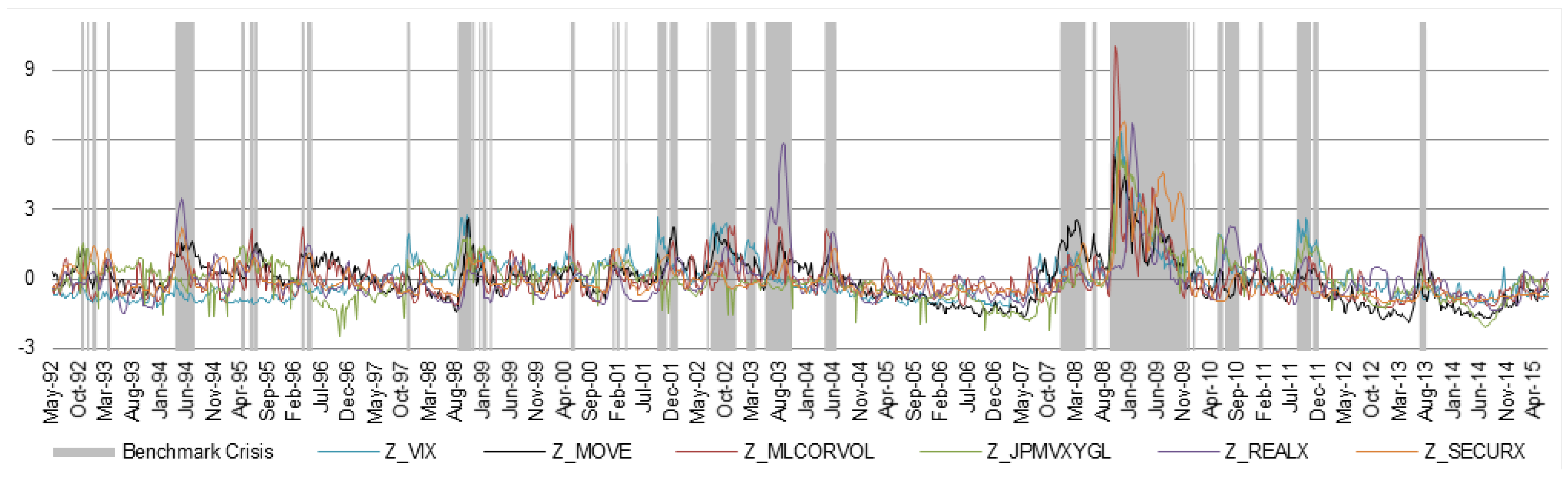
  • 6Namely, we consider the Chicago Board Options Exchange’s VIX, Merrill Lynch’s MOVE, and JP Morgan’s global FX volatility (JPMVXYGL), alongside three calculated volatility measures for corporate bonds, real estate, and securitization from 1 May 1992 to 30 June 2015.
  • 7We select τ B such that approximately 20% of observations will indicate a crisis and fix K = 2, and L = 2.
  • 8The IV metric calculation divides the sample into n bins and becomes unstable if there are not good and bad classifications in each bin.
  • 9Oet et al. [60] recommend selecting τ and μ for each stress measure in order to maximize the relative usefulness of the series.
  • 10The stress period marks the 1973–1975 US crisis that included such momentous events as the fall of the Bretton Woods system, the 1973 oil crisis, the 1973–1975 recession, and the 1973–1974 stock market crash.
  • 11For the equity market several sub-market indicators are not available 1970, and market capitalization data was not found before 1995. Before 1995 we use the earliest available information to infer the size of each sector relative to the set of sectors for which indicator data is available.
  • 12Similarly data is not available to parse out the foreign exchange weight to each country prior to 1977. To enable some historical estimate of stress, the weights for each country from 1977 are applied backwards through 1970.
  • 13Note that the aggregate size of the equity and foreign exchange markets relative to the financial system is available through the Financial Accounts of the US Z.1 Report. However, historical estimates of stress within the equity and foreign exchange markets are naturally limited by the opacity of relative weight within these markets.
  • 14The Bank Holding Company Act of 1956 and Glass–Steagall Act of 1993 prevented US financial intermediaries from expanding their activities to become universal banks.

