Measurement and Modeling of Extra-Column Effects Due to Injection and Connections in Capillary Liquid Chromatography

Abstract

As column volumes continue to decrease, extra-column band broadening has become an increasingly important consideration when determining column performance. Combined contributions due to the injector and connecting tubing in a capillary LC system were measured and found to be larger than expected by Taylor-Aris theory. Variance from sigma-type and tau-type broadening was isolated from eluted peaks using the Foley-Dorsey Exponentially Modified Gaussian peak fitting model and confirmed with computational fluid dynamics. It was found that the tau-type contributions were the main cause for the excessive broadening because of poorly-swept volumes at the connection between the injector and tubing. To reduce tau-type contributions (and peak tailing), a timed pinch mode could be used for analyte injection.

1. Introduction

Since the advent of ultra-high pressure liquid chromatography (UHPLC), particle sizes and column diameters have decreased, leading to smaller column (and, thus, peak) volumes. Consequently, extra-column effects attributed to instrumentation that reduce the measured separation efficiency are more prominent than with standard HPLC columns [1,2,3,4,5,6,7,8,9,10,11]. Similar to previous eras when column technology began to exceed the limitations of commercial equipment [12,13], extra-column band broadening (ECBB) is now seeing increasing attention as an important factor that needs to be accounted for and reduced as much as possible [14,15,16,17,18].

As the column diameter further decreases below 1.0 mm, the impact of the instrumentation on peak bandwidth continues to grow, requiring capillary LC systems with much lower volume [19]. Extra-column effects in these capillary LC (and similar nano-LC) instruments have been described previously [20,21]. In the early development of capillary UHPLC, home-built instruments were constructed that eliminated nearly all instrumental effects and gave a direct measure of column efficiency while also allowing for backpressures in excess of 50,000 psi [22,23,24,25,26,27]. These types of systems are excellent for comparing packing methods or particle types, but most commercial capillary and nano-UHPLC instruments in use today sacrifice these extremely high pressures and negligible extra-column volume for ease of use and range of application (gradient modes, detection methods, etc.). However, these compromises reduce the ability to assess the true chromatographic performance of a column in order to help improve future column design.

When trying to determine the efficiency characteristics of a packed column to describe and compare on-column broadening phenomena, the variance contributions due to extra-column band broadening must be accurately determined so the true plate count can be calculated [28,29]. The most common technique for measuring extra-column effects is by replacing the column with a zero-dead volume (ZDV) connector and observing analyte peak widths using identical experimental conditions (mobile phase composition, flow rate, temperature, and injection volume) [28,30]. This method is the most popular because the existing instrumental set-up is used and observed variances are simply subtracted from the measured peak variance eluted from the column. However, it has been shown that accurately calculating the variance of these extra-column peaks can sometimes prove difficult due to detection limitations [28], challenges selecting proper integration limits for peak moment analysis [31,32,33,34], and discrepancies in the pressure when either the column or ZDV fitting is being measured [35]. An alternative to this “subtraction” method to determine extra-column effects is the use of linear extrapolation [18,36,37,38,39,40,41], where the variance of several analyte peaks with different retention factors are extrapolated back to an intercept that describes the extra-column variance. Others have reported the calculation of extra-column band broadening through graphical analysis or deconvolution of the peak shapes eluted from the column [42,43]. Finally, direct measurements of individual instrument components (where the variance value is found from direct detection without requiring subtraction or extrapolation from other measurements) have been used to help determine the extent of broadening due to specific system elements [44,45] by utilizing techniques commonly employed in flow injection analysis [46,47,48].

In this report, the broadening effects of the injector and inlet connecting tubing were investigated with the goal of determining instrumental variance from these components in a capillary LC system (which have much lower volumes than similar components in standard LC instruments). Compared to a previous study on extra-column band broadening in capillary LC [20], a higher-pressure UHPLC pump was used to expand the flow rate regime that could be investigated and microelectrode electrochemical detection was implemented [48,49] to eliminate effects that detector volume can have on the observed peaks. A novel application of the Foley-Dorsey exponentially-modified Gaussian method [50,51,52] for peak characterization was used to mathematically separate the peak variance from the tubing and the injector. Broadening due to the injector was observed to have a larger value than would be predicted by theoretical equations [14], so computational fluid dynamic (CFD) modeling of the full system was utilized to corroborate the experimental results and gain a better understanding of flow dispersion in the injector system than has previously been available [53]. These findings demonstrate that as the diameter of the connecting tubing increases the measured broadening contributions from not only the tubing, but also the injector (dominated by tau-type broadening) increase. These results reinforce the importance of using the smallest diameter capillary connections possible in capillary LC systems because the increase in variance with larger diameter tubing can be greater than that calculated by the Taylor-Aris equation. Finally, the impacts of a timed pinch injection mode on the reduction of injector broadening and the effects on peak shape when very short tubes are used are discussed.

2. Theory

Theoretical and practical descriptions of ECBB have been detailed previously [14,28,54,55,56,57] and are summarized here for relevant discussion of the results.

2.1. System Contributions to Band Broadening

There are several instrumental contributions that reduce column efficiency. The overall system variance, σ²_tot,sys, is described by the following equation:

$${\sigma }_{tot,sys}^2={\sigma }_{inj}^2+{\tau }_{flow}^2+{\sigma }_{tube}^2+{\sigma }_{det}^2+{\tau }_{data}^2+{\tau }_{filt}^2$$

(1)

where σ² contributions due to the injector (σ²_inj), connecting tubing (σ²_tube), and detector (σ²_det) give Gaussian-type broadening and τ² contributions from mixing volumes (τ²_flow), data acquisition rate (τ²_data), and detector filter rate (τ²_filt) give broadening with an exponential decay nature. This relationship is only valid when all variance values are in either the time or volume domain. These two domains are related through the flow rate (F) as such:

$${\sigma }_{vol}^2={\sigma }_{time}^2\cdot F^2$$

(2)

each system component is further described below (in order based on a standard separation sequence).

2.2. Injector Contributions

The extra-column band broadening effect from the injection plug is usually considered a volumetric contribution based on the volume injected (V_inj):

$${\sigma }_{vol,inj}^2=\frac{V_{inj}^2}{12}$$

(3)

This equation assumes a rectangular plug injection; the value will increase (due to a smaller denominator) as the injected band shape changes [20]. Previous studies of injector design have shown that a good injection requires a narrow, low-volume plug of sample with no poorly swept flow paths [20,53,58,59,60,61,62], which are explained more in the next section.

2.3. Exponential Decay Flow Paths

As an analyte band is transferred from the injector into the connecting tubing, through unions, and into the detector, there can be a number of poorly swept volumes that broaden peaks and cause tailing [63]. The various mass-transport effects present in these systems are rather complex, so the actual effect on system variance (τ²_flow) is a composite of several influences [64]. In column unions and other connectors, these zones act as convective mixing chambers which cause an exponential decay time-dependent broadening contribution, τ_mix:

$${\tau }_{time,mix}^2=t_{mix}^2$$

(4)

with t_mix representing the mean time spent in the mixing chamber [28]. When abrupt changes in tubing radii occur, a related type of mixing volume can arise that is referred to as a diffusion chamber:

$${\tau }_{time,chmbr}^2={\left(\frac{r_{c,1}^2-r_{c,2}^2}{2D_m}\right)}^2$$

(5)

where r_c,1 and r_c,2 are the radii of the two tubes, and D_m is the diffusion coefficient of the analyte [54,64]. Here, convection is absent and the analyte only moves into the flow path through diffusion. No comprehensive description is available for these linked broadening mechanisms, so here they are described as a single exponential decay factor.

2.4. Connecting Tubing

The most common model for broadening in open tubes can generally be written by the Taylor-Aris equation [65,66,67]:

$${\sigma }_{vol,tube}^2=\frac{\pi \cdot L\cdot r_c^4\cdot F}{24D_m}$$

(6)

In this equation, the tube length (L) and the flow rate (F) affect the variance along with the tube radius (r) and the analyte diffusion coefficient. Previous studies have shown this model to be reliable for describing the peak width in open tubes [47,68,69]. For the relationships to hold true the following condition must be met to ensure that the effects of longitudinal convection on solute concentration are negligible [66]:

$$\frac{L}{u_0}>>\frac{r^2}{192D_m}$$

(7)

Golay and Atwood (and others) have explored the regime of broadening in shorter tubes (where this condition is not met) and how a measured band can be skewed due to differences in axial convection and radial diffusion [14,70,71,72]. In these shorter tubes, the measured variance is lower than that predicted by the Taylor-Aris equation. More recently, an exponential-law correction factor was determined that can be applied to Equation 6 to account for these variations [73], although such corrections are not needed when Equation 7 is satisfied, which was the case for the experiments described in Section 4.1, Section 4.2 and Section 4.3. Peak shape variations in this short-tube flow regime are discussed in Section 4.4.

2.5. Detector Contributions

The detector contribution to variance is similar to that for injection volume:

$${\sigma }_{vol,det}^2=\frac{V_{det}^2}{\mathit{12}}$$

(8)

The geometry of the detection cell used in optical detection has been studied in order to maintain high sensitivity while decreasing the overall volume (and variance contribution) [20,74,75,76,77,78,79]. Since this cell can be the most significant contributor to extra-column broadening [15], alternate detection modes have also been surveyed. On-column detection has been employed to eliminate extra tubing requirements, but the low path length tends to hurt sensitivity [56,79,80,81,82,83] and similar measurements using fluorescence require derivatization for many analytes [84,85,86,87]. An alternative option with a low limit of detection and reduced volume is electrochemical detection with a microfiber electrode [49,88,89,90]. The lack of necessary connecting tubing and negligible detector volume make it an effective choice for both measuring and reducing extra-column effects [91].

In addition to Gaussian volumetric broadening, there are time-domain contributions in the detector due to electronic data acquisition (τ_data) and filter (τ_filt) rates:

$${\tau }_{time,data}^2=\frac{t_{samp}^2}{12}$$

(9)

$${\tau }_{time,filt}^2=\frac{t_{filt}^2}{12}=\frac{1}{48{\pi }^2{f}_{filt}^2}$$

(10)

where t_samp and t_filt are the sampling and filter times, and f_filt describes the filter cutoff frequency in inverse time units. When measuring extra-column effects, peak widths are usually very narrow, so a high data acquisition rate must be used to ensure sufficient sampling of the peak (at least 40 points across the peak width) with appropriate filter rates applied (approximately half of the sampling rate) [12,14,28]. In most separations by LC, these conditions are met and time-domain broadening in the detector is limited. However, some LC software can implement digital smoothing than can add significant peak broadening and increase peak variance [92].

2.6. Calculating Peak Variance

Due to the tailing nature of extra-column peaks, half-width methods are not effective in describing the total variance [63]. To effectively determine the variance, the second central statistical moment of the peak must be utilized [54,93]:

$${\sigma }_{var,MoM}^2=\frac{{\displaystyle \underset{t_1}{\overset{t_2}{\int }}{\left(t-t_r\right)}^2\cdot f(t)dt}}{{\displaystyle \underset{t_1}{\overset{t_2}{\int }}f(t)dt}}$$

(11)

where t_r is the peak retention time (first peak moment), f(t) is the measured signal, and t₁ and t₂ are the integration boundaries for the peak. The selection of these integration boundaries can greatly impact the calculated variance value and care must be taken to ensure that an accurate value is obtained [28,31,32,33,34]. One way this has been accomplished is through the use of an iterative method where integration boundaries are set by an initial peak fit, the variance is calculated, the integration limits are expanded incrementally, and the variance value is recalculated [94]. This process iterates until the change in variance per calculation is less than 1%, eliminating bias in selecting the limits of integration and reducing error that comes from selecting limits based on a fraction of the peak maximum [32].

Another widely used method that has been applied for determining the variance of tailing peaks is the Foley-Dorsey model based on an Exponentially-Modified Gaussian (EMG) function [50,51,52]:

$$f(t)=A_{peak}\frac{{\sigma }_{fit}}{{\tau }_{fit}}\sqrt{\frac{\pi }{2}}\exp \left(\frac{{\sigma }_{fit}^2}{2{\tau }_{fit}^2}-\frac{t-t_r}{{\tau }_{fit}}\right)\left(1-erf\left[\frac{1}{\sqrt{2}}\left(\frac{{\sigma }_{fit}}{{\tau }_{fit}}-\frac{t-t_r}{{\sigma }_{fit}}\right)\right]\right)$$

(12)

with the Gaussian “sigma-type” broadening being described by σ_fit, the exponential decay “tau-type” broadening being described by τ_fit, and the peak amplitude represented with A_peak. When using the EMG function to fit peaks, the variance is described by the following equation:

$${\sigma }_{var,EMG}^2={\sigma }_{fit}^2+{\tau }_{fit}^2$$

(13)

3. Experimental Section

3.1. Reagents and Materials

Optima LC-MS grade water and acetonitrile (each containing 0.1% trifluoroacetic acid) were obtained from Fisher Scientific (Waltham, MA, USA). 4-methyl catechol was purchased from Sigma Chemical Company (St. Louis, MO, USA). Silica capillary tubes with 360 µm outer diameter and varying nominal inner diameters (10 µm–50 µm) were purchased from Polymicro Technologies, Inc. (Phoenix, AZ, USA). Capillary end-fittings required 0.0155'' inner diameter (i.d.) PEEK sleeve tubing (IDEX Health and Science, Oak Harbor, WA, USA), stainless steel capillary tubing provided by Waters Corporation, and 1/32'' stainless steel male internal nuts and ferrules (VICI, Houston, TX, USA).

3.2. Direct Measurement Instrumentation and Techniques

The test system consisted of a Waters nanoAcquity binary solvent pump (Milford, MA, USA), four-port 20 nL internal loop injector with associated rotor and actuator (VICI, Houston, TX, USA), a 1 m long segment of capillary (with varied inner diameter), and an electrochemical detector. Prior to analysis, each capillary section was cut to length and polished using a diamond cutting wheel. Then, zero-dead volume high pressure capillary end-fittings were fashioned by sheathing the polished fused silica capillary in PEEK sleeve tubing followed by an outer layer of stainless steel tubing. These three tubes were aligned under microscope, crimped, and then a 1/32'' stainless steel ferrule and male internal nut were used to connect to the injector system. Nominal capillary inner diameters of 20, 30, 40, and 50 µm were reported as 20, 29, 42, and 51 µm by the manufacturer and these values were used for further calculations. The mobile phase used through all experiments was 50% acetonitrile in water (with 0.1% trifluoroacetic acid) and the test analyte was 4-methyl catechol (in the mobile phase). For calculations using the Taylor-Aris equation (Equation 6), the diffusion coefficient of 4-methyl catechol was set at 9.2 × 10⁻⁶ cm²/s (using a previously measured experimental value [95]). For all four diameters, analyte variance was tested at flow rates of 0.5, 1.0, 2.0, 3.0, 4.0, 5.0, 6.0, 7.0, 8.0, 10.0, 12.0, and 15.0 µL/min. Peaks were detected amperometrically using a carbon fiber microfiber electrode (0.3 mm long, 8 µm diameter) inserted directly into the capillary outlet [49]. The current generated was converted to voltage with a SR750 current amplifier (Stanford Research Systems, Sunnyvale, CA, USA). The 3 dB low pass bandwidth filter in the SR750 current amplifier was set to 30 Hz to reduce peak broadening due to the filter (see Figure S1). The start of data acquisition and injection were controlled with signals from the Waters Binary Solvent Manager software. Data was acquired at 80 Hz using a home-built program in LabView 6.0 (National Instruments, Austin, TX, USA).

Peaks were characterized using the EMG fit function in Igor Pro 6.2 (Wavemetrics, Inc., Lake Oswego, OR, USA) so that injector and connecting tubing contributions could be isolated. 3–5 replicates were collected for each measurement (a specific flow rate and inner diameter) and the average values for σ_fit and τ_fit were used (standard deviations were under ~5% for all measurements so error bars are omitted for clarity). Examples of the peak fit and residuals to the raw data can be found in Figure S2. A comparison to the iterative statistical moments (ISM) peak characterization method that has been described previously [94] is detailed in Figure S3.

3.3. Flow Modeling Simulations

Two 3-D models of the injector (rotor, stator, and a 2.5 mm segment of connecting capillary with either 29 or 51 μm i.d.) were generated in COMSOL Multiphysics 4.3 (COMSOL, Inc., Burlington, MA, USA). Streamwise stabilization was employed to reduce ripples in the calculated concentration vs. time plot. The average concentration on the outlet boundary of the 3D model as a function of time was recorded, stored into a file, and used as the inlet boundary condition of a custom Fortran code that solved the 2D axisymmetric convection-diffusion equation in a 99.75 cm long tube of diameter equal to that of the 2.5 mm long tube segment of the 3D model. This two-step solution method was used because it would not have been possible to solve numerically the full 3D problem. The velocity profile in the 99.75 cm long tube was assumed to be parabolic, thus neglecting entrance length effects which are very small in the tube diameters considered in this study. The Fortran program implemented a finite difference alternating direction implicit scheme that is 2nd order accurate in space and time. The same EMG peak-fitting algorithm used for the direct measurement technique was applied to the outputs of both the 3-D injector model and combined 3-D and 2-D model of the whole system. Simulations were run at 1, 3, 5, 7.5, 10, 12.5, and 15 µL/min for each inner diameter.

4. Results and Discussion

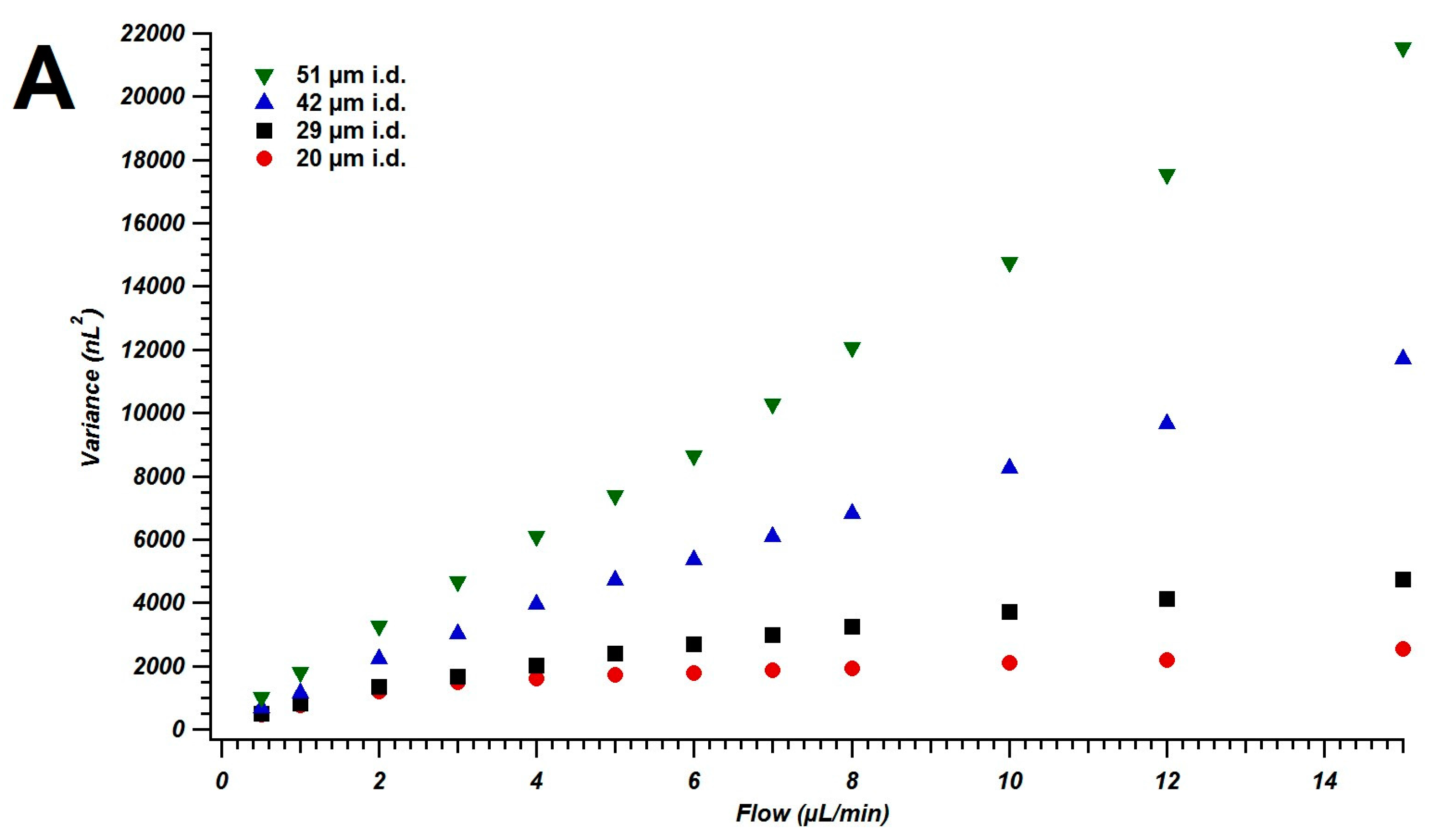
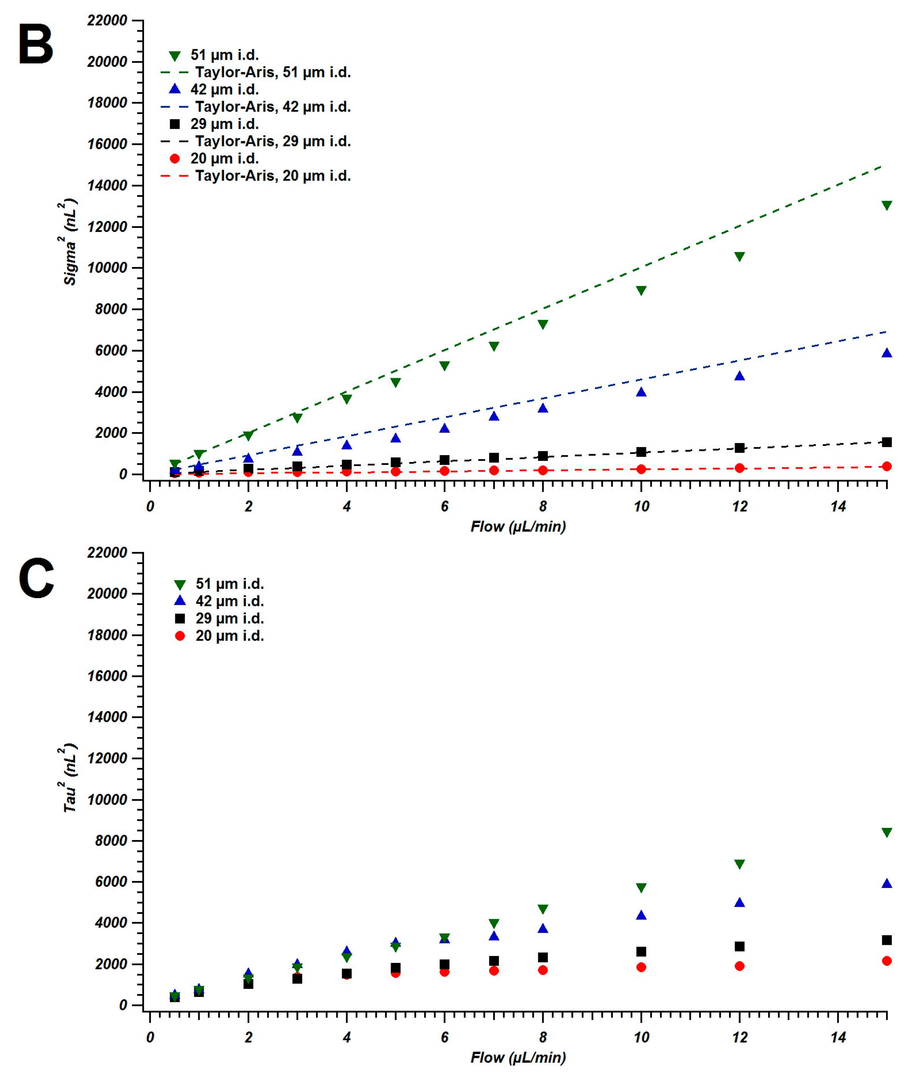
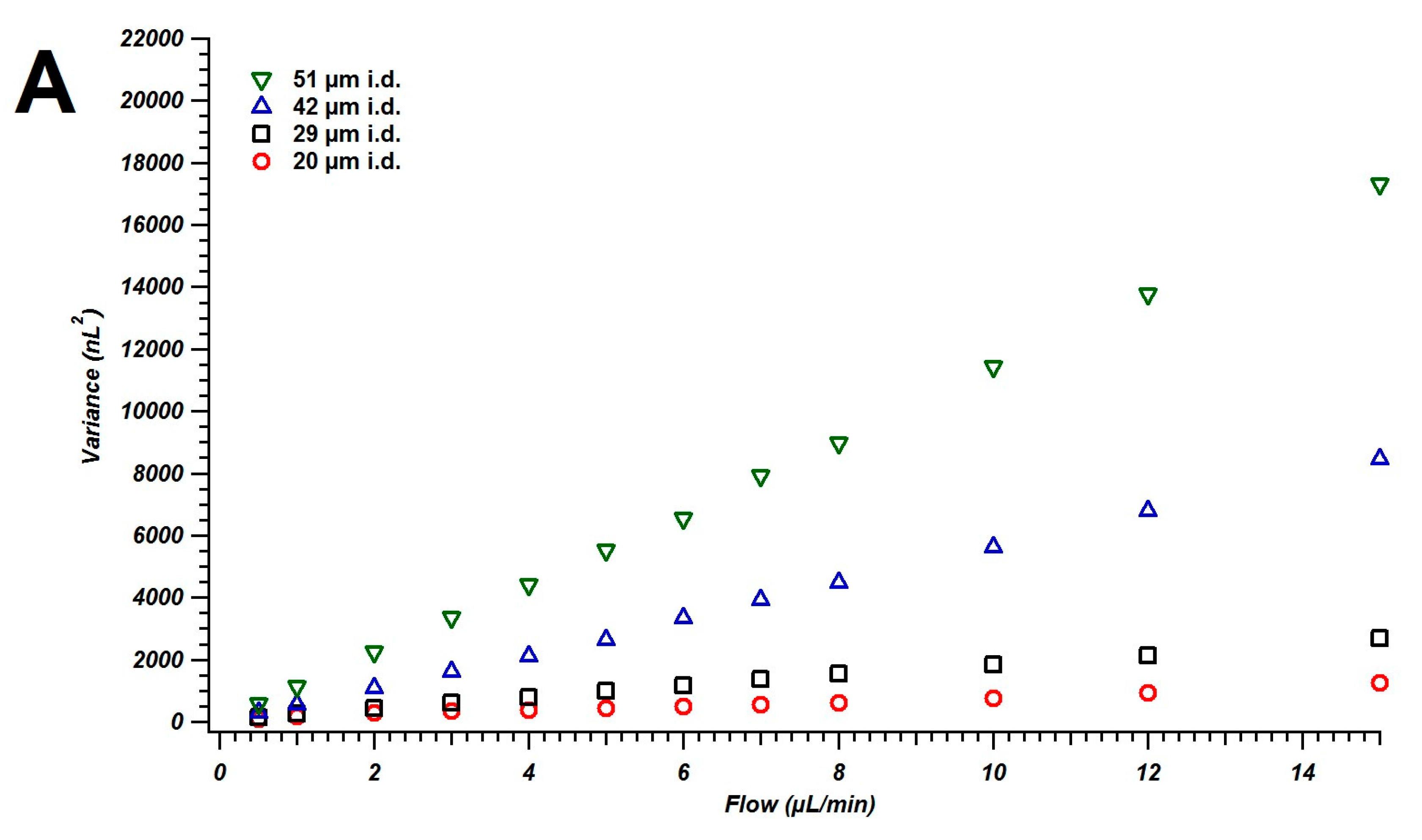
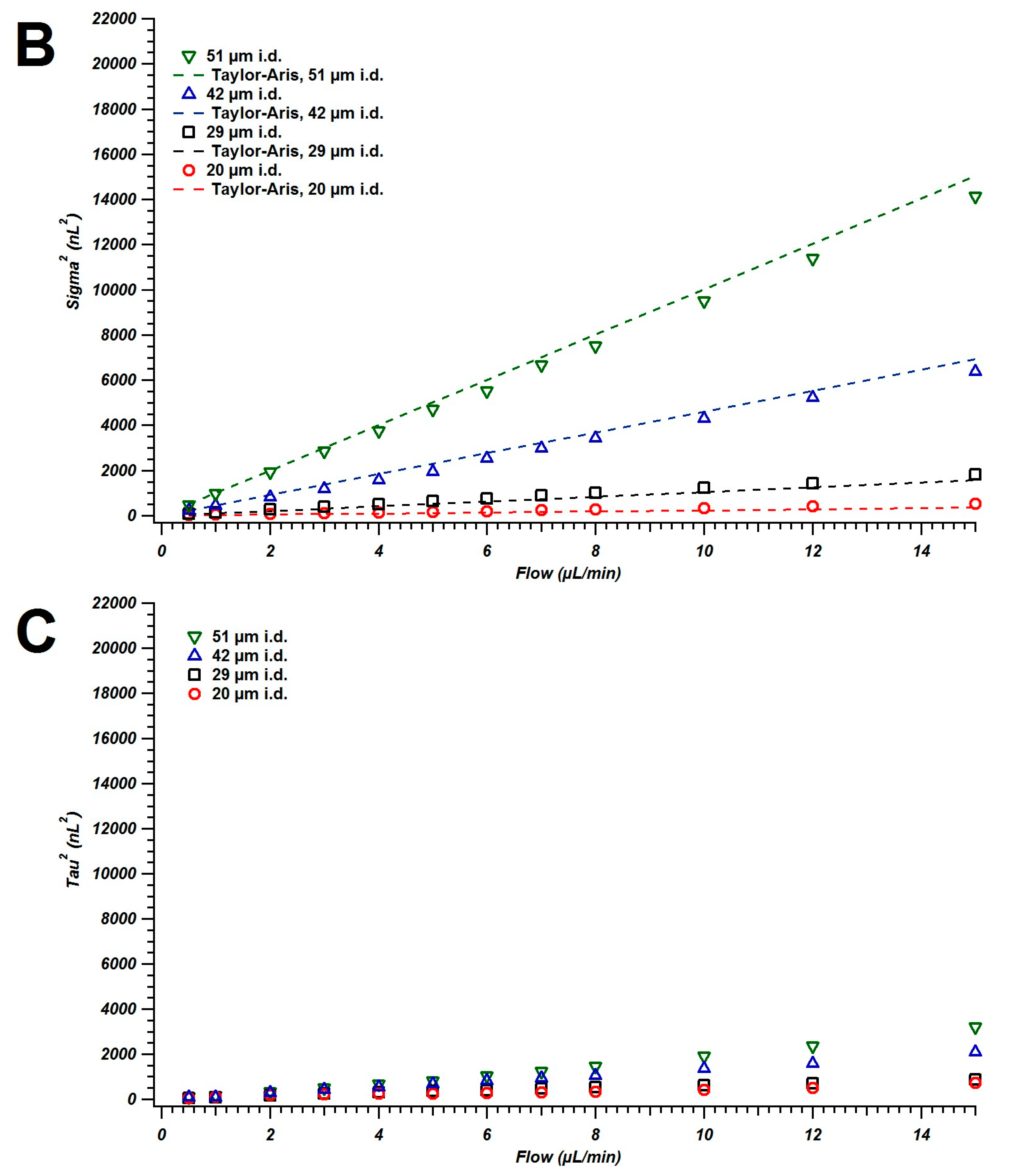
4.1. Broadening in Small Inner Diameter Connecting Capillaries

Due to the low volumes associated with capillary LC columns, connecting tubing diameter is usually limited to the range of 20–50 µm in order to reduce extra-column dispersion effects [96]. In Equation 6, the variance has a fourth-power dependency on the tube radius. Since theory predicts that small changes in this parameter can have a larger impact on instrument broadening than many other factors, variances for tubing diameters within this range were measured using the direct measurement method where a carbon fiber microelectrode was placed directly into the end of the capillary. This method was utilized because there were no extra connecting unions or detection cells that could impact the broadening measurement. 4-methyl catechol was selected as the analyte of choice as its diffusion coefficient has been experimentally measured with the mobile phase and pressures used here [95] and it is detectable using the microelectrode. A Foley-Dorsey type EMG function (Equation 12) was used for peak fitting because it works well for tailing peaks (common when measuring ECBB effects) and because it allows for the separation of Gaussian-type (“sigma-type”) and exponential decay (“tau-type”) broadening.

Figure 1A shows volumetric variances (calculated from Equation 13) for four different small diameter capillaries over a range of flow rates that are typical for capillary LC using sub-2 µm particles. Compared to what might be predicted from Taylor-Aris theory (Equation 6) and mixing volumes in the injector (Equation 4), there are two disparities: (1) the values are higher than expected, and (2) only the largest diameter tubing has a linear nature. To find the origin of the non-linearity of the variance curves of low diameter capillary tubing, contributions from specific instrument components to the overall variance (Equation 1) were assigned to either σ_fit or τ_fit:

$${\sigma }_{fit}^2={\sigma }_{inj}^2+{\sigma }_{tube}^2+{\sigma }_{det}^2$$

(14)

$${\tau }_{fit}^2={\tau }_{flow}^2+{\tau }_{data}^2+{\tau }_{filt}^2$$

(15)

Figure 1. Variance values (obtained from an EMG fit and calculated with Equation 12) measured using the direct measurement method for 20, 29, 42, and 51 µm i.d. capillaries (1 m long) at flow rates ranging from 0.5–15 µL/min are shown in A. Separated sigma-squared and tau-squared values are shown in B and C, respectively. In B, straight-lines indicate values calculated using Taylor-Aris Theory (Equation 6).

Figure 1. Variance values (obtained from an EMG fit and calculated with Equation 12) measured using the direct measurement method for 20, 29, 42, and 51 µm i.d. capillaries (1 m long) at flow rates ranging from 0.5–15 µL/min are shown in A. Separated sigma-squared and tau-squared values are shown in B and C, respectively. In B, straight-lines indicate values calculated using Taylor-Aris Theory (Equation 6).

With the components of the system used for these direct measurements and predictions from Equations 3, 7, 8, and 9, the maximum contributions from some parameters were taken to be negligible at most variance values shown in Figure 1A: injector (33 nL²), detector (0.03 nL²), data filter rate (0.15 nL²), and data acquisition rate (0.8 nL²). By removing these contributions from Equations 14 and 15, σ_fit and τ_fit are estimated to reflect specific instrument components:

$${\sigma }_{fit}^2\approx {\sigma }_{tube}^2$$

(16)

$${\tau }_{fit}^2\approx {\tau }_{flow}^2$$

(17)

To determine the accuracy of the approximation in Equation 16, theoretical values for tube broadening calculated by Equation 6 were compared to the calculated values for σ²_fit (Figure 1B). For all capillary inner diameters the sigma-type broadening closely matches the theoretical values predicted by Equation 6, although the difference between the two is larger as the radius grows. Because this is the case, Equation 17 allows for a description of convective (Equation 4) and diffusional (Equation 5) broadening modes that can both contribute to tau-type broadening. Since the only connection in the system tested was at the injector, all tau-type contributions can be attributed to the injector. τ²_fit values between 0.5 and 15 µL/min for all four capillary diameters are shown in Figure 1C. In the lower diameters, there is a roll-off nature to the data points while at 51 µm i.d. the τ²_fit values are nearly linear. When using the EMG function, the variance is a sum of σ² and τ² (Equation 13) so the increased curvature in Figure 1A at lower diameters can be attributed to the greater influence of the injector at smaller inner diameters (leading to greater observed peak tailing). As the magnitude of the sigma-type broadening from the open tube grows quickly with increasing inner diameter (such as the 51 µm i.d. capillary data in Figure 1B), the fraction of the variance due to the injector is reduced and the data appears more linear.

Atwood and Golay suggested that one component that may act as a “low-plate limit”-type broadening mechanism is the injector [71]. At higher flow rates there would be less time for equilibration of the peak and the distribution of the injected profile would change (see further discussion on peak profile observations in Section 4.4). This shorter equilibration time can lead to some of the leveling off [28]. Equation 4 shows that part of the tau contribution is related to the time of mixing in the internal loop after the valve is switched, which when shifted to the volume domain with Equation 2 gives a constant value across the flow rate range equal to V²_inj. Even though the injector output should be the same for all capillary tubing used, there is an abrupt diameter change when eluting from the 100 µm channel of the injector stator to the capillary tube. At this abrupt change, there is expected to be a contribution to tau-type variance that is flow rate independent and grows as the difference in diameter increases [54,64]. However, the experimental values for tau contributions are much lower than those calculated by Equation 5. Furthermore, the values are flow-rate dependent, and the magnitude grows as the diameter of the tubing increases, which is contrary to this equation). The data measured here shows that the actual exponential decay-like nature of these peaks falls somewhere between a strictly diffusion-controlled and strictly mixing-controlled value. But, the observed trends are the opposite of what might be expected from a diffusion chamber. To further explore the complex nature of these ECBB measurements and corroborate the findings, CFD modeling was utilized and is described in the following section.

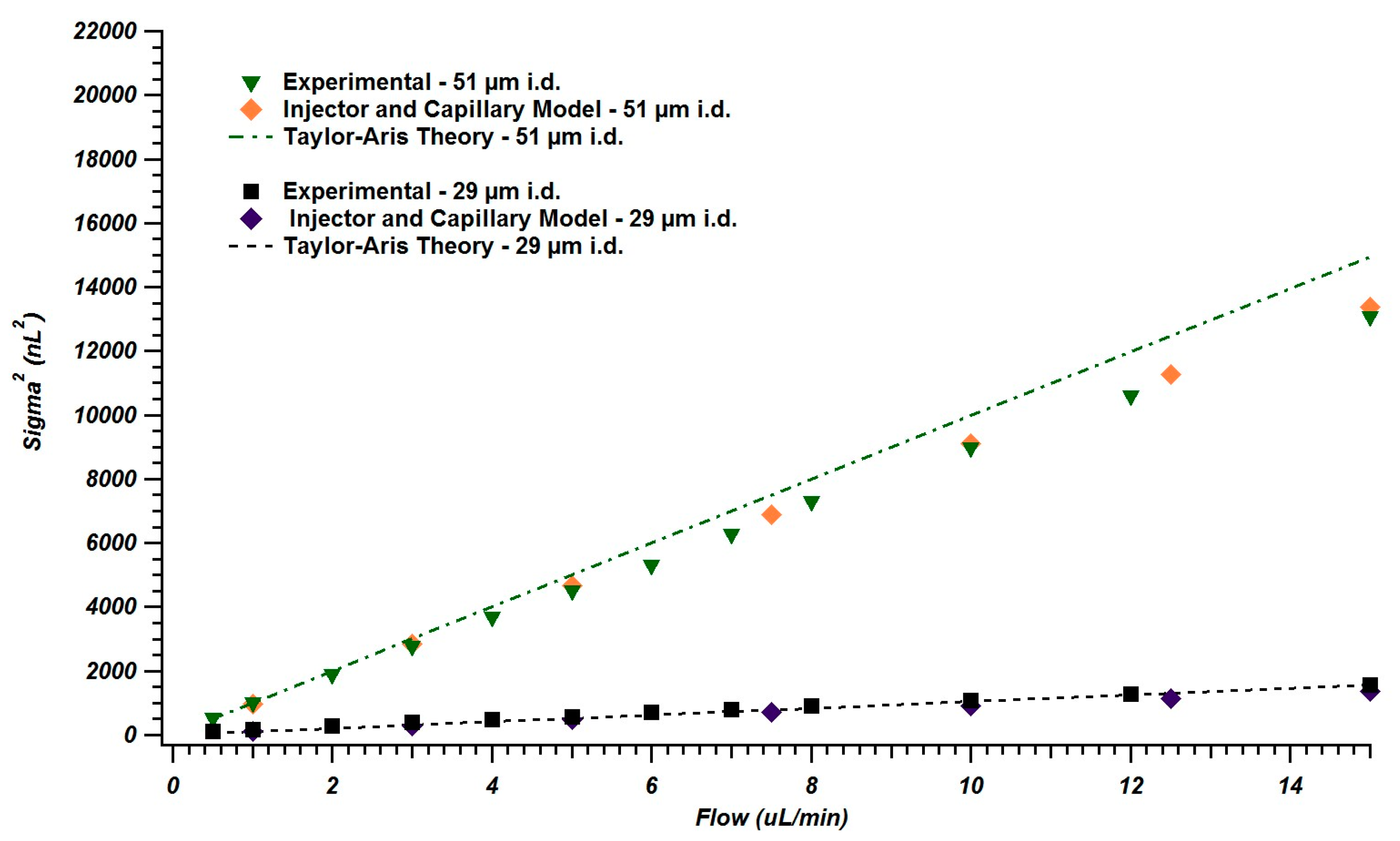
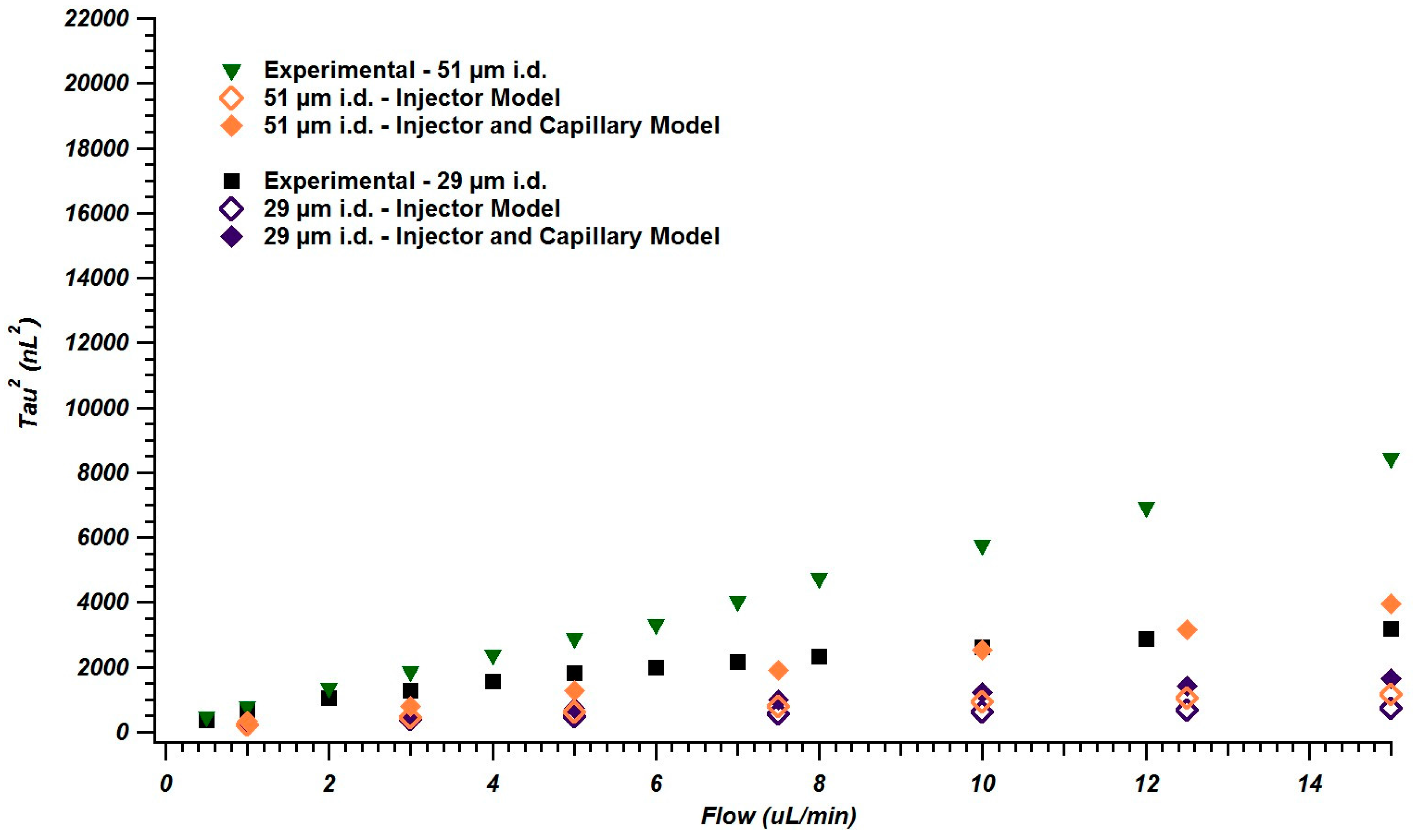
4.2. Simulations of Broadening in Injectors and Connecting Tubing

CFD modeling has been employed for injector simulations (1-D and 2-D) on large volume systems using COMSOL [97]. However, such a model on a complete injector/tubing system in capillary LC or a comparison to experimental measurements has yet to be explored [20]. Computational limits and calculation requirements preclude the use of a full 3-D model of the entire injector and capillary system, so simplifications were made to maintain accuracy but reduce the number of required calculations. First, a 3-D model of the injector rotor (containing the internal loop) and stator was designed based on manufacturer diagrams. This model included a 2.5 mm segment of connecting capillary so that tau-type effects that may arise due to the abrupt diameter change would be accounted for. The concentration vs. time plot out of this initial model was then used as the input profile into a 2-D axisymmetric model of 99.75 cm length to replicate the experimental set-up. Due to the long computation times, only two models were investigated (both simulated across the flow rate range): A smaller diameter (29 µm) and larger diameter (51 µm) tube.

Concentration vs. time peak profiles were characterized with the same EMG algorithm that was used to measure the peaks from the direct measurement method. Peaks at the end of both the 2.5 mm and 1 m segment of capillary tubing were measured to compare how σ²_fit and τ²_fit changed at both positions. At the outlet of the 3-D axisymmetric model σ² was negligible (<10 nL²) and at the outlet of the entire model σ² was found to match Taylor-Aris predictions and the experimental data (Figure 2). This demonstrates that the σ values isolated from the EMG peak fit for both the experimental and simulated data sets match what would be predicted by Taylor-Aris theory. Thus, additional variance contributions in both the experimental and modeled data beyond those from the connecting tubing are dominated by τ. τ² for both CFD models and the experimental data from the direct measurement technique are compared in Figure 3. An initial look at the magnitudes of experimental and simulated τ values shows that the measured tau-type broadening is much higher than that of the models. This may be due to inaccuracies in the geometry of the model where misalignment in the actual rotor and stator could cause additional broadening. Another reason may be due to mechanical motion of the injector because flow in the model begins with the inlet already aligned while in the actual injector it must move into place during the position switch. It must be noted that when shifting the output profile from the 3-D model to the 2-D model the concentration profile is re-equilibrated radially, but this re-equilibration does not happen in the actual experiment. One explanation of the tailing effect growing with increasing inner diameter is based on how analyte moves from the loop, through the stator, and into the capillary tubing. As the initial flow brings most of the analyte down the center of the channel, some of the sample fluid remains stagnant at the abrupt diameter change and only slowly moves into the channel along the wall. In larger diameters, the flow velocity is slower at the wall and it requires a longer diffusional path to reach the fastest velocities at the center of the channel, hence the greater tailing factor. This radial fidelity is lost when shifting between the 3-D and 2-D axisymmetric models and is likely the main reason this data shifts from the experimental values.

Despite these inaccuracies, some observations on the actual transport of analyte out of the injection loop can be made. At lower flow rates the calculated τ² values at the outlet of the injector and the connected capillary are similar, but the difference between them grows as the flow rate increases. It is at these higher flow rates where Taylor-Aris broadening (Equation 6) would be expected to have a larger impact on the measured variance. The increasing gap between τ² at the injector outlet and capillary outlet indicates that magnification of the broadening between these two components could be occurring due to a lack of mixing when the flow path is uninterrupted (and as analyte in the peak tail stays closer to the wall). This creates a peak profile with a higher tau value as the diameter grows. Additionally, since the Taylor-Aris broadening is larger in the 51 µm i.d. tubing, then the difference between τ² after 2.5 mm and after 1 m is expected to be greater (because of the larger “operator” value) than that in the 29 µm i.d. tubing. This is also observed in Figure 3, showing that trends that would be expected based on the experimental data are supported by CFD modeling.

Figure 2. Comparison of sigma-squared for experimental data, COMSOL simulated data, and Taylor-Aris Theory (Equation 6) for 29 and 51 µm i.d. capillaries (1 m long).

Figure 2. Comparison of sigma-squared for experimental data, COMSOL simulated data, and Taylor-Aris Theory (Equation 6) for 29 and 51 µm i.d. capillaries (1 m long).

Figure 3. Comparison of tau-squared for experimental data and COMSOL simulated data (following just the injector and the combined injector and connecting tubing) for 29 and 51 µm i.d. capillaries (1 m long).

Figure 3. Comparison of tau-squared for experimental data and COMSOL simulated data (following just the injector and the combined injector and connecting tubing) for 29 and 51 µm i.d. capillaries (1 m long).

If components are not mutually independent (through re-equilibration by mixing), then larger extra-column “operators” (in this case, capillary tubing with a larger diameter) could increase the band-spreading of the input profile [60]. For larger volume systems, small dead volumes in connecting unions allow for re-equilibration and ensure this independence, leading to lower variance contributions [71]. The broadening contribution that these unions create in capillary LC systems is much more significant and must be avoided with direct connections, making this combined injector-tubing effect an important factor to consider in instrument design (specifically the couplings and diameters of fluidic paths).

4.3. Reducing Tau-Type Broadening with Pinch Injections

In addition to the full loop injection mode described in the previous sections, a timed pinch injection mode was also tested to see how the broadening contribution from the system changed. In the timed pinch injection mode, the injector loop switches in and out of the flow path for a given time interval (100 ms in these experiments) which can reduce the injection of analyte molecules trapped in poorly swept volumes and thereby decrease peak tailing (see Section SI3 for discussion regarding effects of this injection style on injected volume). Figure 4 shows variance, sigma-squared, and tau-squared data measured after 1 m of capillary when such an injection method is used. In Figure 4C, the τ² values for the four capillary diameters are shown when this alternate injection mode is utilized. The magnitude of the injector contribution to variance is also much higher for the full injection than the pinch injection (as demonstrated by the smallest tau contributor (20 µm i.d.) from Figure 1C and the value in Figure 4C) while the sigma contributions are similar to Taylor-Aris theory in both cases. When comparing 20 µm i.d. data at 15 µL/min, using the pinch injection reduces τ² by two-thirds when compared to the full injection value. By eliminating the rear boundary of the injection profile with the switch, a significant portion of the dispersion that occurs due to tau-type broadening in the injector is reduced [20,53]. Additionally, the eluted peaks have less tailing than when the full loop injection mode is used. Since the connecting tubing can magnify broadening from the injector, using pinch injections can dramatically reduce ECBB, especially when using very small diameter connecting tubing.

Figure 4. Variance values (obtained from an EMG fit and calculated with Equation 12) measured using the direct measurement method for 20, 29, 42, and 51 µm i.d. capillaries (1 m long) for the timed pinch injection at flow rates ranging from 0.5–15 µL/min are shown in A. Separated sigma-squared and tau-squared values when using the timed pinch injection are shown in B and C, respectively. In B, straight-lines indicate values calculated using Taylor-Aris Theory (Equation 6).

Figure 4. Variance values (obtained from an EMG fit and calculated with Equation 12) measured using the direct measurement method for 20, 29, 42, and 51 µm i.d. capillaries (1 m long) for the timed pinch injection at flow rates ranging from 0.5–15 µL/min are shown in A. Separated sigma-squared and tau-squared values when using the timed pinch injection are shown in B and C, respectively. In B, straight-lines indicate values calculated using Taylor-Aris Theory (Equation 6).

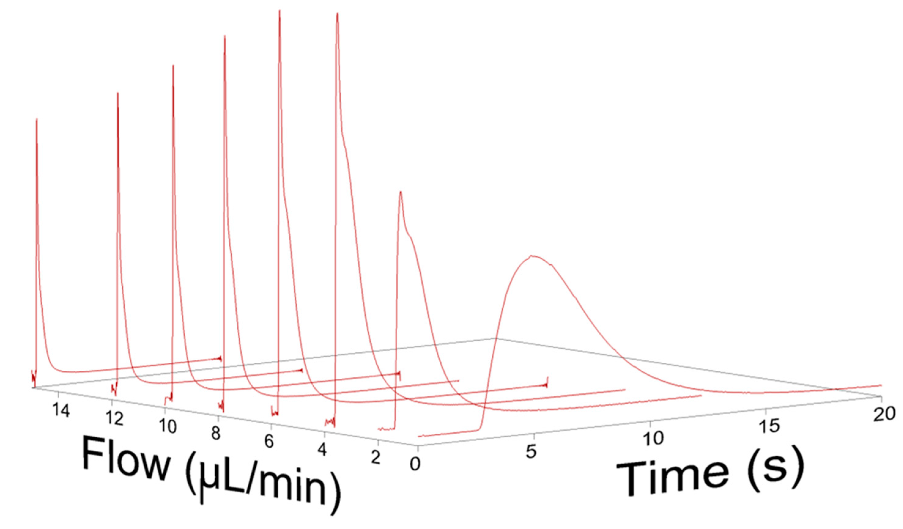
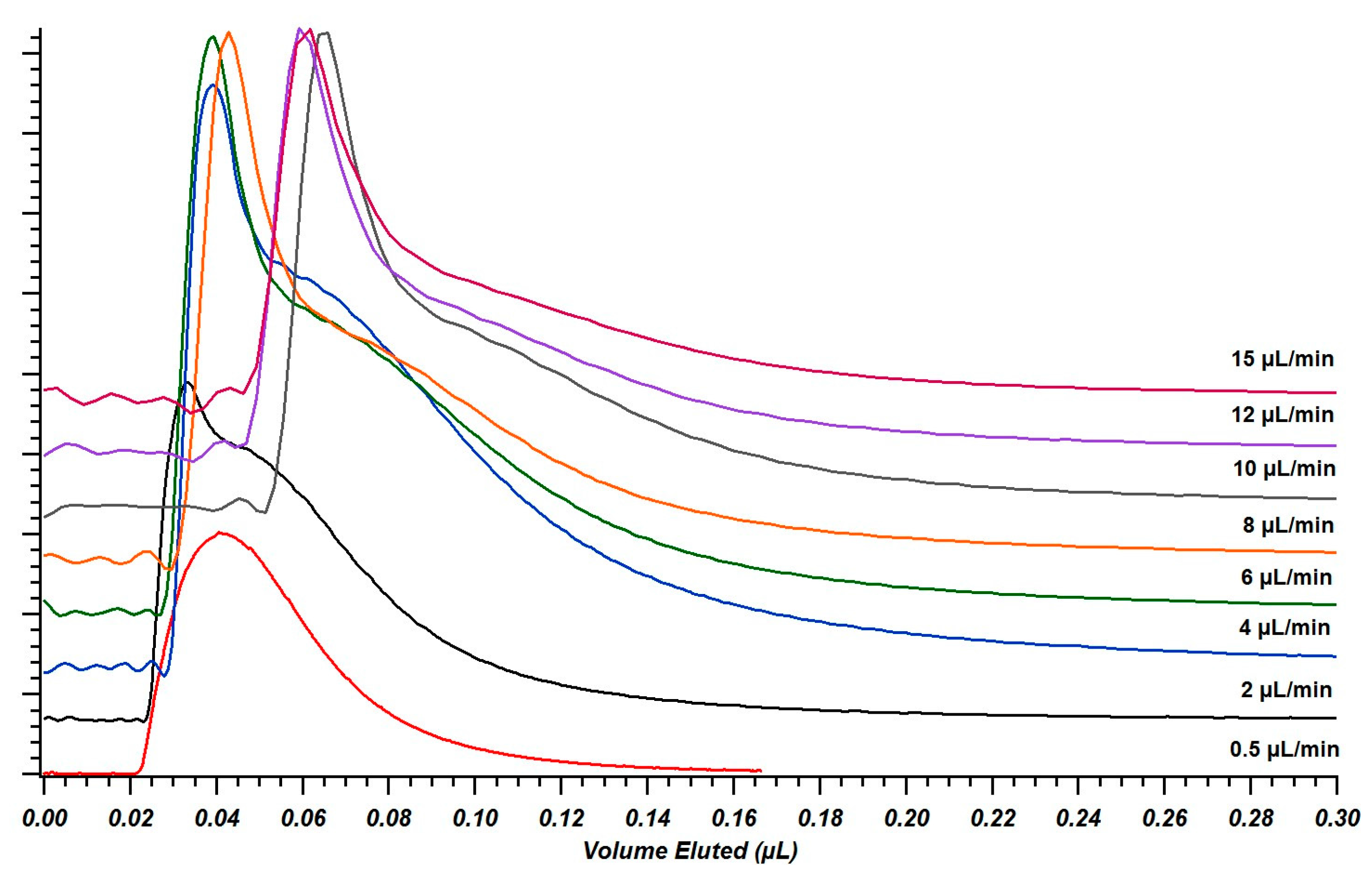
4.4. Injector Elution Profiles

By modifying the direct measurement set-up, peak injections were measured to determine the solute output profile into the connecting capillary. A similar set-up of measuring injector output with a small volume connecting capillary has previously been described using conductivity detection [53]. Injection profiles using the full loop injection mode are shown in Figure 5. At low flow rates, the peaks have some tailing but are smooth. As the flow rate is increased, a shoulder begins to form and is present throughout the remainder of the peak profiles up to flow rates of 15 µL/min. This general trend follows the peak profile for the low-plate limit in short tubes described previously by Golay and Atwood [70,71]. When there is an insufficient sampling of the flow profile due to limited diffusion time (high velocities in short tubes), asymmetrical distributions arise. The observation of these band shapes directly out of the injector indicates that the actual output of the sample loop generally operates in a low-plate limit domain. In this case, the dispersion that would be predicted by Equation 6 would overestimate the true value measured at the injector outlet [98]. In the injector design, the 100 µm stator channel acts as a short tube where Taylor-Aris broadening would be lower than expected and would be another negligible contribution to the τ² value (Equation 17). Thus, the flow non-idealities in the injector that contribute to the tau-type broadening observed here (Section 4.1 and Section 4.2) are the dominant contribution to total broadening when Taylor-Aris broadening is minimal (i.e., the smallest diameter tubing).

Figure 5. Peak injection profiles of a full loop injection measured out of the injector through a small (6 cm, 13 µm inner diameter) connecting capillary for eight flow rates between 0.5 and 15 µL/min in the time domain.

Figure 5. Peak injection profiles of a full loop injection measured out of the injector through a small (6 cm, 13 µm inner diameter) connecting capillary for eight flow rates between 0.5 and 15 µL/min in the time domain.

When normalizing the peaks to their eluted volume (rather than time) in Figure 6, the general growth of the tailing portion of the peak as the flow rate grows becomes more apparent. The distribution profile of the analyte peak changes with the flow rate due to decreases in equilibration time (analyte molecules in the center of the tube are traveling faster than those at the wall and at higher flow rates there is not enough time for molecules to sufficiently sample all flow paths and “average” the peak shape) [28,98]. After a meter long segment of tubing, the flow profile distortions are relaxed by diffusion and lead to the peak profiles that were characterized for variance in this article.

Figure 6. Peak injection profiles of a full loop injection measured out of the injector through a small (6 cm, 13 µm inner diameter) connecting capillary for eight flow rates between 0.5 and 15 µL/min in the volumetric domain.

Figure 6. Peak injection profiles of a full loop injection measured out of the injector through a small (6 cm, 13 µm inner diameter) connecting capillary for eight flow rates between 0.5 and 15 µL/min in the volumetric domain.

5. Conclusions

Based on the results demonstrated here (both experimental and computational), it is clear that the contributions to extra-column band broadening that might be expected due to an injector in a capillary LC system are much greater than what Equation 3 would predict. This is due to flow paths where analyte transport is modified (mainly at sharp diameter changes where tubing connections are made), which increases the peak variance. This broadening is exacerbated by connecting tubing between the injector and column because the initial tailed peak “input profile” is not re-equilibrated when proper connections are made, resulting in a magnification of tau-type broadening. This indicates that the requirement for small diameter connecting tubing in capillary LC systems is actually greater than would be expected (based on the volume contributions in Equation 6) when trying to limit instrumental effects. For more complex analyses where capillary LC columns are coupled to mass spectrometers, mobile phase gradients are typically employed. While the pre-column broadening effects investigated here are reduced for analytes that are highly retained under initial gradient conditions [99], the band variance of early eluting compounds with little to no retention will still decrease if smaller diameter tubing and timed pinch injections are employed. Along with using columns that are longer or packed with smaller particles, this need for smaller diameter connecting tubing demonstrates another motivation to increase pressure limits in capillary LC systems. Furthermore, by using a timed pinch injection the impact of poorly mixed volumes can be greatly reduced which helps improve the shape of the injected peak profile and reduces the observed chromatographic peak widths.

References

1. Gritti, F.; Guiochon, G. On the extra-column band-broadening contributions of modern, very high pressure liquid chromatographs using 2.1 mm I.D. columns packed with sub-2 μm particles. J. Chromatogr. A 2010, 1217, 7677–7689. [Google Scholar] [CrossRef] [PubMed]
2. Wu, N.; Bradley, A.C.; Welch, C.J.; Zhang, L. Effect of extra-column volume on practical chromatographic parameters of sub-2-μm particle-packed columns in ultra-high pressure liquid chromatography. J. Sep. Sci. 2012, 35, 2018–2025. [Google Scholar] [CrossRef] [PubMed]
3. Gritti, F.; Sanchez, C.A.; Farkas, T.; Guiochon, G. Achieving the full performance of highly efficient columns by optimizing conventional benchmark high-performance liquid chromatography instruments. J. Chromatogr. A 2010, 1217, 3000–3012. [Google Scholar] [CrossRef] [PubMed]
4. Fekete, S.; Fekete, J. The impact of extra-column band broadening on the chromatographic efficiency of 5 cm long narrow-bore very efficient columns. J. Chromatogr. A 2011, 1218, 5286–5291. [Google Scholar] [CrossRef] [PubMed]
5. Gritti, F.; Leonardis, I.; Shock, D.; Stevenson, P.; Shalliker, A.; Guiochon, G. Performance of columns packed with the new shell particles, Kinetex-C18. J. Chromatogr. A 2010, 1217, 1589–1603. [Google Scholar] [CrossRef] [PubMed]
6. Heinisch, S.; Desmet, G.; Clicq, D.; Rocca, J.-L. Kinetic plot equations for evaluating the real performance of the combined use of high temperature and ultra-high pressure in liquid chromatography: Application to commercial instruments and 2.1 and 1 mm I.D. columns. J. Chromatogr. A 2008, 1203, 124–136. [Google Scholar] [CrossRef] [PubMed]
7. Lestremau, F.; Wu, D.; Szücs, R. Evaluation of 1.0 mm i.d. column performances on ultra high pressure liquid chromatography instrumentation. J. Chromatogr. A 2010, 1217, 4925–4933. [Google Scholar] [CrossRef] [PubMed]
8. Omamogho, J.O.; Hanrahan, J.P.; Tobin, J.; Glennon, J.D. Structural variation of solid core and thickness of porous shell of 1.7 μm core-shell silica particles on chromatographic performance: Narrow bore columns. J. Chromatogr. A 2011, 1218, 1942–1953. [Google Scholar] [CrossRef] [PubMed]
9. Wu, N.; Bradley, A.C. Effect of column dimension on observed column efficiency in very high pressure liquid chromatography. J. Chromatogr. A 2012, 1261, 113–120. [Google Scholar] [CrossRef] [PubMed]
10. Gritti, F.; Guiochon, G. Rapid development of core-shell column technology: Accurate measurements of the intrinsic column efficiency of narrow-bore columns packed with 4.6 down to 1.3 µm superficially porous particles. J. Chromatogr. A 2014, 1333, 60–69. [Google Scholar] [CrossRef] [PubMed]
11. Buckenmaier, S.; Miller, C.A.; van de Goor, T.; Dittmann, M.M. Instrument contributions to resolution and sensitivity in ultra high performance liquid chromatography using small bore columns: Comparison of diode array and triple quadrupole mass spectrometry detection. J. Chromatogr. A 2015, 1377, 64–74. [Google Scholar] [CrossRef] [PubMed]
12. Martin, M.; Eon, C.; Guiochon, G. Study of the pertinency of pressure in liquid chromatography: II. Problems in equipment design. J. Chromatogr. A 1975, 108, 229–241. [Google Scholar] [CrossRef]
13. Reese, C.E.; Scott, R.P.W. Microbore columns—Design, construction, and operation. J. Chromatogr. Sci. 1980, 18, 479–486. [Google Scholar] [CrossRef]
14. Fountain, K.J.; Neue, U.D.; Grumbach, E.S.; Diehl, D.M. Effects of extra-column band spreading, liquid chromatography system operating pressure, and column temperature on the performance of sub-2-μm porous particles. J. Chromatogr. A 2009, 1216, 5979–5988. [Google Scholar] [CrossRef] [PubMed]
15. Gritti, F.; Guiochon, G. On the minimization of the band-broadening contributions of a modern, very high pressure liquid chromatograph. J. Chromatogr. A 2011, 1218, 4632–4648. [Google Scholar] [CrossRef] [PubMed]
16. Alexander, A.J.; Waeghe, T.J.; Himes, K.W.; Tomasella, F.P.; Hooker, T.F. Modifying conventional high-performance liquid chromatography systems to achieve fast separations with Fused-Core columns: A case study. J. Chromatogr. A 2011, 1218, 5456–5469. [Google Scholar] [CrossRef] [PubMed]
17. Gritti, F.; Guiochon, G. The current revolution in column technology: How it began, where is it going? J. Chromatogr. A 2012, 1228, 2–19. [Google Scholar] [CrossRef] [PubMed]
18. Gritti, F.; Guiochon, G. Accurate measurements of the true column efficiency and of the instrument band broadening contributions in the presence of a chromatographic column. J. Chromatogr. A 2014, 1327, 49–56. [Google Scholar] [CrossRef] [PubMed]
19. Gritti, F.; Guiochon, G. Kinetic performance of narrow-bore columns on a micro-system for high performance liquid chromatography. J. Chromatogr. A 2012, 1236, 105–114. [Google Scholar] [CrossRef] [PubMed]
20. Prüß, A.; Kempter, C.; Gysler, J.; Jira, T. Extracolumn band broadening in capillary liquid chromatography. J. Chromatogr. A 2003, 1016, 129–141. [Google Scholar] [CrossRef]
21. Chervet, J.P.; Ursem, M.; Salzmann, J.P. Instrumental requirements for nanoscale liquid chromatography. Anal. Chem. 1996, 68, 1507–1512. [Google Scholar] [CrossRef] [PubMed]
22. MacNair, J.E.; Lewis, K.C.; Jorgenson, J.W. Ultrahigh-pressure reversed-phase liquid chromatography in packed capillary columns. Anal. Chem. 1997, 69, 983–989. [Google Scholar] [CrossRef] [PubMed]
23. MacNair, J.E.; Patel, K.D.; Jorgenson, J.W. Ultrahigh-pressure reversed-phase capillary liquid chromatography: Isocratic and gradient elution using columns packed with 1.0-micron particles. Anal. Chem. 1999, 71, 700–708. [Google Scholar] [CrossRef] [PubMed]
24. Patel, K.D.; Jerkovich, A.D.; Link, J.C.; Jorgenson, J.W. In-depth characterization of slurry packed capillary columns with 1.0-microm nonporous particles using reversed-phase isocratic ultrahigh-pressure liquid chromatography. Anal. Chem. 2004, 76, 5777–5786. [Google Scholar] [CrossRef] [PubMed]
25. Mellors, J.S.; Jorgenson, J.W. Use of 1.5-μm Porous Ethyl-Bridged Hybrid Particles as a Stationary-Phase Support for Reversed-Phase Ultrahigh-Pressure Liquid Chromatography. Anal. Chem. 2004, 76, 5441–5450. [Google Scholar] [CrossRef] [PubMed]
26. Lippert, J.A.; Xin, B.; Wu, N.; Lee, M.L. Fast ultrahigh-pressure liquid chromatography: On-column UV and time-of-flight mass spectrometric detection. J. Microcol. Sep. 1999, 11, 631–643. [Google Scholar] [CrossRef]
27. Wu, N.; Lippert, J.A.; Lee, M.L. Practical aspects of ultrahigh pressure capillary liquid chromatography. J. Chromatogr. A 2001, 911, 1–12. [Google Scholar] [CrossRef]
28. Gritti, F.; Felinger, A.; Guiochon, G. Influence of the errors made in the measurement of the extra-column volume on the accuracies of estimates of the column efficiency and the mass transfer kinetics parameters. J. Chromatogr. A 2006, 1136, 57–72. [Google Scholar] [CrossRef] [PubMed]
29. Gritti, F.; Guiochon, G. Mass transfer kinetics, band broadening and column efficiency. J. Chromatogr. A 2012, 1221, 2–40. [Google Scholar] [CrossRef] [PubMed]
30. Freebairn, K.W.; Knox, J.H. Dispersion measurements on conventional and miniaturised HPLC systems. Chromatographia 1984, 19, 37–47. [Google Scholar] [CrossRef]
31. Gritti, F.; Guiochon, G. Accurate measurements of peak variances: Importance of this accuracy in the determination of the true corrected plate heights of chromatographic columns. J. Chromatogr. A 2011, 1218, 4452–4461. [Google Scholar] [CrossRef] [PubMed]
32. Verstraeten, M.; Liekens, A.; Desmet, G. Accurate determination of extra-column band broadening using peak summation. J. Sep. Sci. 2012, 35, 519–529. [Google Scholar] [CrossRef] [PubMed]
33. Stevenson, P.G.; Gao, H.; Gritti, F.; Guiochon, G. Removing the ambiguity of data processing methods: optimizing the location of peak boundaries for accurate moment calculations. J. Sep. Sci. 2013, 36, 279–287. [Google Scholar] [CrossRef] [PubMed]
34. Stevenson, P.G.; Gritti, F.; Guiochon, G. Automated methods for the location of the boundaries of chromatographic peaks. J. Chromatogr. A 2011, 1218, 8255–8263. [Google Scholar] [CrossRef] [PubMed]
35. Gritti, F.; Guiochon, G. Effect of the pressure on pre-column sample dispersion theory, experiments, and practical consequences. J. Chromatogr. A 2014, 1352, 20–28. [Google Scholar] [CrossRef] [PubMed]
36. Kok, W.T.; Brinkman, U.A.T.; Frei, R.W.; Hanekamp, H.B.; Nooitgedacht, F.; Poppe, H. Use of conventional instrumentation with microbore column in high-performance liquid chromatography. J. Chromatogr. A 1982, 237, 357–369. [Google Scholar] [CrossRef]
37. Claessens, H.A.; Cramers, C.A.; Kuyken, M.A.J. Estimation of the band broadening contribution of HPLC equipment to column elution profiles. Chromatographia 1987, 23, 189–194. [Google Scholar] [CrossRef]
38. Dezaro, D.A.; Dvorn, D.; Horn, C.; Hartwick, R.A. Time optimization for routine separations, using high-speed microbore HPLC. Chromatographia 1985, 20, 87–96. [Google Scholar] [CrossRef]
39. Claessens, H.A.; Hetem, M.J.J.; Leclercq, P.A.; Cramers, C.A. Estimation of the instrumental band broadening contribution to the column elution profiles in open tubular capillary liquid chromatography. J. High Res. Chromatogr. 1988, 11, 176–180. [Google Scholar] [CrossRef]
40. Rebscher, H.; Pyell, U. A method for the experimental determination of contributions to band broadening in electrochromatography with packed capillaries. Chromatographia 1994, 38, 737–743. [Google Scholar] [CrossRef]
41. Prüß, A.; Kempter, C.; Gysler, J.; Jira, T. Evaluation of packed capillary liquid chromatography columns and comparison with conventional-size columns. J. Chromatogr. A 2004, 1030, 167–176. [Google Scholar] [CrossRef] [PubMed]
42. Nilsson, O. On the estimation of extra-column contributions to band broadening through measurements on an authentic chromatogram. J. High Res. Chromatogr. 1979, 2, 605–608. [Google Scholar] [CrossRef]
43. Wright, N.A.; Villalanti, D.C.; Burke, M.F. Fourier transform deconvolution of instrument and column band broadening in liquid chromatography. Anal. Chem. 1982, 54, 1735–1738. [Google Scholar] [CrossRef]
44. Beisler, A.T.; Schaefer, K.E.; Weber, S.G. Simple method for the quantitative examination of extra column band broadening in microchromatographic systems. J. Chromatogr. A 2003, 986, 247–251. [Google Scholar] [CrossRef]
45. Hupe, K.-P.; Jonker, R.J.; Rozing, G. Determination of band-spreading effects in high-performance liquid chromatographic instruments. J. Chromatogr. A 1984, 285, 253–265. [Google Scholar] [CrossRef]
46. Reijn, J.M.; Van der Linden, W.E.; Poppe, H. Some theoretical aspects of flow injection analysis. Anal. Chim. Acta 1980, 114, 105–118. [Google Scholar] [CrossRef]
47. Reijn, J.M.; Van der Linden, W.E.; Poppe, H. Transport phenomena in flow injection analysis without chemical reaction. Anal. Chim. Acta 1980, 126, 1–13. [Google Scholar] [CrossRef]
48. Kristensen, E.W.; Wilson, R.L.; Wightman, R.W. Dispersion in flow injection analysis measured with microvoltammetric electrodes. Anal. Chem. 1986, 58, 986–988. [Google Scholar] [CrossRef]
49. Knecht, L.A.; Guthrie, E.J.; Jorgenson, J.W. On-column electrochemical detector with a single graphite fiber electrode for open-tubular liquid chromatography. Anal. Chem. 1984, 56, 479–482. [Google Scholar] [CrossRef]
50. Foley, J.P.; Dorsey, J.G. Equations for calculation of chromatographic figures of merit for ideal and skewed peaks. Anal. Chem. 1983, 55, 730–737. [Google Scholar] [CrossRef]
51. Foley, J.P.; Dorsey, J.G. A Review of the Exponentially Modified Gaussian (EMG) Function: Evaluation and Subsequent Calculation of Universal Data. J. Chromatogr. Sci. 1984, 22, 40–46. [Google Scholar] [CrossRef]
52. Jeansonne, M.S.; Foley, J.P. Review of the Exponentially Modified Gaussian (EMG) Function Since 1983. J. Chromatogr. Sci. 1991, 29, 258–266. [Google Scholar] [CrossRef]
53. Foster, M.D.; Arnold, M.A.; Nichols, J.A.; Bakalyar, S.R. Performance of experimental sample injectors for high-performance liquid chromatography microcolumns. J. Chromatogr. A 2000, 869, 231–241. [Google Scholar] [CrossRef]
54. Sternberg, J.C. Extracolumn Contributions to Chromatographic Band Broadening. In Advances in Chromatography; Giddings, J., Keller, R.A., Eds.; Marcel Dekker: New York, NY, USA, 1966; Volume 2, pp. 205–270. [Google Scholar]
55. Poppe, H. Column liquid chromatography. In Journal of Chromatography Library; Heftmann, E., Ed.; Elsevier: New York, NY, USA, 1992; Volume 51A, pp. A151–A225. [Google Scholar]
56. Vissers, J.P.C.; Claessens, H.A.; Cramers, C.A. Microcolumn liquid chromatography: Instrumentation, detection and applications. J. Chromatogr. A 1997, 779, 1–28. [Google Scholar] [CrossRef]
57. Vissers, J.P.C. Recent developments in microcolumn liquid chromatography. J. Chromatogr. A 1999, 856, 117–143. [Google Scholar] [CrossRef]
58. Colin, H.; Martin, M.; Guiochon, G. Extra-column effects in high-performance liquid chromatography: I. Theoretical study of the injection problem. J. Chromatogr. A 1979, 185, 79–95. [Google Scholar] [CrossRef]
59. Schmid, A. Sample injection in liquid chromatography. Chromatographia 1979, 12, 825–829. [Google Scholar] [CrossRef]
60. Lauer, H.H.; Rozing, G.P. The selection of optimum conditions in HPLC I. The determination of external band spreading in LC instruments. Chromatographia 1981, 14, 641–647. [Google Scholar] [CrossRef]
61. Claessens, H.A.; Burcinova, A.; Cramers, C.A.; Mussche, P.; van Tilburg, C.C.E. Evaluation of injection systems for open tubular liquid chromatography. J. Microcol. Sep. 1990, 2, 132–137. [Google Scholar] [CrossRef]
62. Bakalyar, S.R.; Phipps, C.; Spruce, B.; Olsen, K. Choosing sample volume to achieve maximum detection sensitivity and resolution with high-performance liquid chromatography columns of 1.0, 2.1 and 4.6 mm I.D. J. Chromatogr. A 1997, 762, 167–185. [Google Scholar] [CrossRef]
63. Stankovich, J.J.; Gritti, F.; Stevenson, P.G.; Guiochon, G. The impact of column connection on band broadening in very high pressure liquid chromatography. J. Sep. Sci. 2013, 36, 2709–2717. [Google Scholar] [CrossRef] [PubMed]
64. Lucy, C.A.; Giavina, L.L.M.; Cantwell, F.F. A Laboratory Experiment on Extracolumn Band Broadening in Liquid Chromatography. J. Chem. Educ. 1995, 72, 367–374. [Google Scholar] [CrossRef]
65. Taylor, G. Dispersion of soluble matter in solvent flowing slowly through a tube. P. Roy. Soc. A 1953, 219, 186–203. [Google Scholar] [CrossRef]
66. Taylor, G. Conditions under which dispersion of a solute in a stream of solvent can be used to measure molecular diffusion. P. Roy. Soc. A 1954, 225, 473–477. [Google Scholar] [CrossRef]
67. Aris, R. On the dispersion of a solute in a fluid flowing through a tube. P. Roy. Soc. A 1956, 235, 67–77. [Google Scholar] [CrossRef]
68. Shankar, A.; Lenhoff, A.M. Dispersion in round tubes and its implications for extracolumn dispersion. J. Chromatogr. A 1991, 556, 235–248. [Google Scholar] [CrossRef]
69. Liu, G.; Svenson, L.; Djordjevic, N.; Erni, F. Extra-column band broadening in high-temperature open-tubular liquid chromatography. J. Chromatogr. A 1993, 633, 25–30. [Google Scholar] [CrossRef]
70. Golay, M.J.E.; Atwood, J.G. Early phases of the dispersion of a sample injected in poiseuille flow. J. Chromatogr. A 1979, 186, 353–370. [Google Scholar] [CrossRef]
71. Atwood, J.G.; Golay, M.J.E. Dispersion of peaks by short straight open tubes in liquid chromatography systems. J. Chromatogr. A 1981, 218, 97–122. [Google Scholar] [CrossRef]
72. Vrentas, J.S.; Vrentas, C.M. Dispersion in laminar tube flow at low Peclet numbers or short times. AIChE J. 1988, 34, 1423–1430. [Google Scholar] [CrossRef]
73. Broeckhoven, K.; Desmet, G. Numerical and analytical solutions for the column length-dependent band broadening originating from axisymmetrical trans-column velocity gradients. J. Chromatogr. A 2009, 1216, 1325–1337. [Google Scholar] [CrossRef] [PubMed]
74. Scott, R.P.W.; Kucera, P. Mode of operation and performance characteristics of microbore columns for use in liquid chromatography. J. Chromatogr. A 1979, 169, 51–72. [Google Scholar] [CrossRef]
75. Kahle, V.; Krejčí, M. Role of extra-column volume in the efficiency of high-speed liquid chromatography. J. Chromatogr. A 1985, 321, 69–79. [Google Scholar] [CrossRef]
76. Brooks, H.B.; Thrall, C.; Tehrani, J. High-performance liquid chromatography system for packed capillary columns. J. Chromatogr. A 1987, 385, 55–64. [Google Scholar] [CrossRef]
77. Chervet, J.P.; Ursem, M.; Salzmann, J.P.; Vanoort, R.W. Ultra-sensitive UV detection in micro separation. J. High Res. Chromatogr. 1989, 12, 278–281. [Google Scholar] [CrossRef]
78. Kamahori, M.; Watanabe, Y.; Miura, J.; Taki, M.; Miyagi, H. High-sensitivity micro ultraviolet absorption detector for high-performance liquid chromatography. J. Chromatogr. A 1989, 465, 227–232. [Google Scholar] [CrossRef]
79. Bruin, G.J.M.; Stegeman, G.; van Asten, A.C.; Xu, X.; Kraak, J.C.; Poppe, H. Optimization and evaluation of the performance of arrangements for UV detection in high-resolution separations using fused-silica capillaries. J. Chromatogr. A 1991, 559, 163–181. [Google Scholar] [CrossRef]
80. Yang, F.J. On-column detection using a fused silica column. J. High Res. Chromatogr. 1981, 4, 83–85. [Google Scholar] [CrossRef]
81. Walbroehl, Y.; Jorgenson, J.W. On-column UV absorption detector for open tubular capillary zone electrophoresis. J. Chromatogr. A 1984, 315, 135–143. [Google Scholar] [CrossRef]
82. Kientz, C.; Verweij, A. Construction of a UV cell for micro-liquid chromatography. J. High Res. Chromatogr. 1988, 11, 294–296. [Google Scholar] [CrossRef]
83. Vindevogel, J.; Schuddinck, G.; Dewaele, C.; Verzele, M. Simple instrument modification for packed fused silica capillary or micro-LC: Evaluation on the use of tubular UV-detection cells. J. High Res. Chromatogr. 1988, 11, 317–321. [Google Scholar] [CrossRef]
84. Kucera, P.; Umagat, H. Design of a post-column fluorescence derivatization system for use with microbore columns. J. Chromatogr. A 1983, 255, 563–579. [Google Scholar] [CrossRef]
85. Guthrie, E.J.; Jorgenson, J.W. On-column fluorescence detector for open-tubular capillary liquid chromatography. Anal. Chem. 1984, 56, 483–486. [Google Scholar] [CrossRef]
86. Rose, D.J., Jr.; Jorgenson, J.W. Post-capillary fluorescence detection in capillary zone electrophoresis using o-phthaldialdehyde. J. Chromatogr. A 1988, 447, 117–131. [Google Scholar] [CrossRef]
87. Nickerson, B.; Jorgenson, J.W. Characterization of a post-column reaction—laser-induced fluorescence detector for capillary zone electrophoresis. J. Chromatogr. A 1989, 480, 157–168. [Google Scholar] [CrossRef]
88. Manz, A.; Simon, W. Picoliter Cell Volume Potentiometric Detector for Open-Tubular Column LC. J. Chromatogr. Sci. 1983, 21, 326–330. [Google Scholar] [CrossRef]
89. White, J.G.; St. Claire, R.L., III; Jorgenson, J.W. Scanning on-column voltammetric detector for open-tubular liquid chromatography. Anal. Chem. 1986, 58, 293–298. [Google Scholar] [CrossRef] [PubMed]
90. Manz, A.; Simon, W. Potentiometric detector for fast high-performance open-tubular column liquid chromatography. Anal. Chem. 1987, 59, 74–79. [Google Scholar] [CrossRef]
91. Baur, J.E.; Kristensen, E.W.; Wightman, R.W. Radial dispersion from commercial high-performance liquid chromatography columns investigated with microvoltammetric electrodes. Anal. Chem. 1988, 60, 2334–2338. [Google Scholar] [CrossRef] [PubMed]
92. Felinger, A.; Kilár, A.; Boros, B. The myth of data acquisition rate. Anal. Chim. Acta 2015, 854, 178–182. [Google Scholar] [CrossRef] [PubMed]
93. Grushka, E.; Myers, M.N.; Schettler, P.D.; Giddings, J.C. Computer characterization of chromatographic peaks by plate height and higher central moments. Anal. Chem. 1969, 41, 889–892. [Google Scholar] [CrossRef]
94. Hsieh, S.; Jorgenson, J.W. Preparation and Evaluation of Slurry-Packed Liquid Chromatography Microcolumns with Inner Diameters from 12 to 33 μm. Anal. Chem. 1996, 68, 1212–1217. [Google Scholar] [CrossRef] [PubMed]
95. Kaiser, T.J.; Thompson, J.W.; Mellors, J.S.; Jorgenson, J.W. Capillary-Based Instrument for the Simultaneous Measurement of Solution Viscosity and Solute Diffusion Coefficient at Pressures up to 2000 bar and Implications for Ultrahigh Pressure Liquid Chromatography. Anal. Chem. 2009, 81, 2860–2868. [Google Scholar] [CrossRef] [PubMed]
96. Noga, M.; Sucharski, F.; Suder, P.; Silberring, J. A practical guide to nano-LC troubleshooting. J. Sep. Sci. 2007, 30, 2179–2189. [Google Scholar] [CrossRef] [PubMed]
97. Samuelsson, J.; Edström, L.; Forssén, P.; Fornstedt, T. Injection profiles in liquid chromatography. I. A fundamental investigation. J. Chromatogr. A 2010, 1217, 4306–4312. [Google Scholar] [CrossRef] [PubMed]
98. Gritti, F.; McDonald, T.; Gilar, M. Accurate measurement of dispersion data through short and narrow tubes used in very high-pressure liquid chromatography. J. Chromatogr. A 2015, 1410, 118–128. [Google Scholar] [CrossRef] [PubMed]
99. Gilar, M.; McDonald, T.S.; Johnson, J.S.; Murphy, J.P.; Jorgenson, J.W. Wide injection zone compression in gradient reversed-phase liquid chromatography. J. Chromatogr. A 2015, 1390, 86–94. [Google Scholar] [CrossRef] [PubMed]