Article

Design and Verification of Cyber-Physical Systems Specified by Petri Nets—A Case Study of a Direct Matrix Converter

by
Remigiusz Wisniewski
*,
Grzegorz Bazydło
,
Paweł Szcześniak
,
Iwona Grobelna
and
Marcin Wojnakowski
Institute of Electrical Engineering, University of Zielona Gora, Szarfrana 2, 65-516 Zielona Gora, Poland
*
Author to whom correspondence should be addressed.
Mathematics 2019, 7(9), 812; https://doi.org/10.3390/math7090812
Submission received: 28 July 2019 / Revised: 16 August 2019 / Accepted: 29 August 2019 / Published: 2 September 2019

Abstract

:
The paper proposes a novel design technique of cyber-physical systems (CPSs). The system is specified by a Petri net, and further modelled in a hardware description language (HDL) towards final implementation in a programmable device. Contrary to the traditional design methods, the proposed solution is highly focused on the verification aspects. The system is checked three times before the final implementation in hardware. Initially, the Petri-net based specification is formally verified by the application of the model-checking technique. Secondly, software verification of the modelled system is performed. Finally, the hardware verification of the already implemented system is executed. The proposed method is explained by an example of a direct matrix converter (MC) with transistor commutation and space vector modulation (SVM). The main benefits, as well as the limitations, of the proposed solution are discussed and analysed.

1. Introduction

A cyber-physical system (CPS) [1,2] integrates cybernetic aspects together with physical processes. Embedded computers monitor and control physical processes, usually with feedback loops, and physical processes affect the computations [1]. Sensors within the system allow to sense the surrounding physical environment and react accordingly through control and actuator modules with a physical change in the system [3]. A CPS consists therefore of a set of modules that cooperate with each other. Those modules usually operate in a concurrent manner, allowing execution of multiple operations simultaneously. CPSs can be observed in almost all areas of human life, e.g., vehicular and transportation systems, social networks and gaming, medical and health-care systems, smart homes and buildings, power and thermal management systems, electric power grids and energy systems [4,5,6,7,8,9,10,11,12].
The design of CPS is a structured creation of artefacts and specifies how a system is realising its main tasks [1]. In the paper we focus on the control part of a CPS system, that is on the control logic responsible for appropriate tasks execution in response to the events occurring within or outside the system. Generally, the control algorithm of a CPS can be specified in many ways, as in the embedded systems design [13], using e.g., Petri nets [3,14] or diagrams of the unified modelling language (UML) [15]. Hybrid automata, combining discrete and continuous aspects, can also be applied [16]. In the domain of arising cyber-physical systems, similar approaches can be found. A comprehensive survey paper [10] discusses several modelling techniques, semantics and programming tools for design of CPSs, concerning e.g., model-driven development (MDD). Generalised stochastic Petri nets are proposed in [2] to model cyber-physical manufacturing systems, focusing especially on the trustworthiness. Indeed, the approach is said to be effective to model and analyse the trustworthiness of the manufacturing CPS. Coloured spatiotemporal Petri nets are used in [17] to model transportation of CPS. Petri nets are also applied in [18] to describe information security risk evaluation process. A UML software profile for CPS applications is presented in [19], as an introduction of basic steps of a methodology for deploying CPS applications at a high level of programming.
In this work, live and safe Petri nets are proposed for the formal description of the CPS [3,20,21,22]. Such an approach has several advantages. First of all, it naturally reveals concurrency relations in the system [23]. Moreover, it is supported by methods and tools that allows for advanced analysis [24,25] and formal verification of the CPS [26]. Additionally, the reliability and robustness of the design [27,28] can be analysed. Furthermore, advanced decomposition techniques can be applied in order to implement the system among the distributed devices [29]. The design method shown in the paper highly focuses on the validation and verification aspects of the control part of CPS, in particular concerning formal verification (with the model checking technique) and analysis of the specification, software verification (using dedicated simulation programs) and hardware verification (with test-scenarios and measurement of the control signals).
Let us present the most interesting design and modelling methods of cyber-physical systems. The importance of design and modelling of CPSs is highlighted in the survey paper [30], with an overview of different types of systems and appearing challenges. The design of CPSs requires integrated design methods considering all engineering disciplines and focusing also on integration and interaction of separate physical and computational components [30,31]. Design automation tools should be developed to facilitate the multi-disciplinary collaboration [32].
Another survey paper [33] shows the potential benefits of the convergence between several technologies. It also discusses various design methods, starting from the early stages of computing and assembler code, through high level programming languages (C and Fortran), object-oriented programming languages (C++ and Java), model-driven development (MDD), model-driven architecture (MDA) and ending with model-integrated computing (MIC). The current state of the art related to CPS systems, especially regarding model-based methodologies, is presented in [34]. Modelling techniques addressing only software aspects are not able to accurately specify CPSs. The paper aims to be a basis for future extensions of the SysML standard to support CPS modelling.
A model-integrated development approach that addresses the development needs of CPS through the pervasive use of models is introduced in [35], covering all aspects of hardware and software components with their interactions. The elements of the framework are either already available or the technology for them is available. The proposed modelling language (EsMoL) is used to specify hardware platform and software components models.
A cyber-physical production framework (CyProF) for designing CPS-based solutions in production environments is proposed in [36]. Architecture components classes (ACCs) are defined to model production systems in detail, which can be realised using common modelling languages, like UML or business process model and notation (BPMN).
Graph-based design languages based on diagrams of UML for product development process are discussed in [37], using an example of complex automotive components. The paper presents an interesting case study of an automotive bonnet—an example for a complete automation of the entire product development process. An approach towards fully automated generation of CAD models is introduced, with fewer interfaces between modelling and simulation tools.
The MDD approach of software-intensive CPS (siCPS) is addressed in [38]. It is stated that traditional model-driven design and development techniques cannot ensure both the dependability and the self-adaptivity in the dynamic environments. A novel model-based design process is proposed which comprises both appropriate methods and models and allows for early implementations. The invariant refinement method (IRM) is introduced, integrated into the ensemble development life cycle.
A high-level architecture description language (ADL) for modelling CPSs within the INSAC framework is proposed in [39]. In ADL both borders and bindings between system components are declared. Additionally, scalable runtime environment interactions are described in the INSAC prescription language (IPL) and the INSAC modelling language (IML) is used to describe the dynamic of the system.
Let us now shortly discuss the state-of-the-art in the area of cyber-physical systems verification. In particular, we will focus on the approaches similar to the one proposed in this paper. Some classical methods from software and hardware verification can be adapted and applied on CPS systems [40]. The overview of verification and validation aspects of CPS is presented in [41]. The paper shows a qualitative literature review, but also an online survey of 25 CPS researchers and interviews with nine practitioners. It concludes that existing formal and simulation methods are insufficient for supporting the development of general-purpose CPS. Additionally, classical software engineering approaches are evaluated as not applicable directly to CPS.
The correctness of the cyber-physical composition verified by means of a model-checking technique is shown in [42]. The idea is supported by an advanced electric power grid example (and the Real-Time SPIN tool with Real-Time Promela input language). It has to be pointed out that each component may function correctly independently, yet the composition of several modules may yield incorrectness due to the interference. The system is logically decomposed into smaller modules to reduce the state explosion problem and consequently to allow it to be efficiently checked.
In [43] BNDC (bi-simulation-based non-deducibility on compositions) properties of CPS, being a variant of non-interference properties are formally verified using model checking and the security process algebra (SPA). Furthermore, statistical model checking of CPS (especially useful for verifying systems with very large state spaces) is discussed in [44]. It is shown that the Importance Sampling and the Cross-Entropy methods can be used to solve the rare event problem. Statistical model checking combines the Monte Carlo method with temporal logic model checking.
Authors in [45] propose that CPS should be modelled and verified online. It is shown how to build online models that describe the time-bounded short-run behaviour of CPS. Such models ought to be built in a short time to guarantee discovering any faults or failures before they happen and to provide as much time as possible for the online systems to react.
In [46] an automatic abstraction methodology simplifying CPS models is proposed. The models are described by a user-defined language and then automatically compiled into a LHPN (labelled hybrid Petri net) model. The LHPN model represents software and hardware, together with environment in a single formalism. Moreover, LHPN transformations permits for reduction of the model complexity [46]. The verification tool called LEMA is used to support automatic transformation, compilation, and models verification.
Summarising the above discussion, it should be noted that existing formal and simulation methods are insufficient for supporting the development of CPS. There is a lack of prototyping flows of the cyber-part of the CPSs focused on the verification of the designed system. The existing techniques usually apply external tools and converters or require dedicated models or languages.
This paper introduces a novel design methodology of the control part of the cyber-physical system described by a safe and live Petri net. The presented technique is strongly oriented toward the validation and verification aspects of the system, especially the control part of the CPS.
In the proposed verification-oriented approach, the designed system is checked three times. First, formal verification methods are used to verify the CPS at the early specification step. Such aspects are important, as early formal verification allows increasing of final quality of the prototyped CPS, decreasing of costs and shortening of system development time. Validation of the specification ensures that the designed CPS meets all requirements, which are important for the user or customer. It is possible to define and verify both the behavioural and the structural properties of the analysed CPS. However, it should be noted that only those properties which have been previously defined can be checked. This means that the requirements list should be as complete and versatile as possible. The additional advantages of the model checking technique are the generated counterexamples that allow tracing of undesired situations and simplifying of the error localisation. Thanks to the uncomplicated rule-based logical model, formal verification of the specification is simplified and more intuitive, what is an important aspect for CPS developers [47].
Second verification (software validation) is performed at the modelling stage. The correct functionality of the designed algorithms is checked using dedicated simulation programs by performing the numeric experiment. Finally, after the implementation of the control algorithm in a programmable devices-like field programmable gate arrays (FPGAs) the hardware verification is done. The correctness of the implemented algorithm is verified by performing test-scenarios and measuring the control signals.
The presented approach is illustrated by a real example of direct matrix converter (MC). In particular, the complete design methodology of an MC with transistor commutation and space vector modulation (SVM) oriented for further implementation in a programmable device is presented.
The main contributions can be summarised as follows:
  • A novel design technique of a control part of a cyber-physical system specified by a live and safe Petri net is proposed in the paper. The proposed idea is oriented toward the hardware implementation of the CPS. Contrary to similar design methods, the presented approach highly utilises verification aspects of the designed system, especially the control part of the CPS;
  • The system is verified three times during the prototyping process. Initially, a model-checking and analysis of the primary specification is performed. Secondly, the software verification of the modelled system is executed. Eventually, the CPS is once more examined, after the final implementation in hardware;
  • The proposed method does not apply external tools (except MATLAB/Simulink), nor any additional conversions. In particular, any model-checking tool can be used in order to perform a formal verification of the system. Moreover, analysis of the system can be done with the application of any known methods that allow examination of the main properties of a Petri net (liveness, safeness, reachability, etc.). Furthermore, there are no restrictions regarding software verification, since any known HDL-simulator can be applied to produce data for further analysis in MATLAB/Simulink software;
  • The proposed technique is explained by a case-study example of a direct matrix converter (MC) with transistor commutation and space vector modulation (SVM). The system is specified by a safe and live Petri net, described in the Verilog hardware description language and finally implemented in an FPGA device. Based on the MC example, also the usefulness of the proposed verification-oriented approach is shown.
The paper is structured as follows. Section 2 is focused on the theoretical background, where aspects related to Petri nets and matrix converters are presented. The idea of the proposed design technique is explained in Section 3, while Section 4 illustrates the presented approach by a case-study example. Finally, Section 5 summarises the paper and presents directions for future works.

2. Theoretical Background

This section presents notations and theoretical aspects required to explain the proposed technique. Firstly, we shall introduce definitions that refer to Petri net theory [25,26,48,49,50,51,52,53]. Subsequently, an algorithm of matrix converter with space vector modulation (SVM) will be shown.

2.1. Petri Nets

Petri nets are one of the popular forms of graphical representation and specification of control systems. They turn out to be especially effective in the area of analysis, design, and verification of logic controllers. The notations presented below correspond to the definitions from [25,26,48,49,50,51,52,53].
Definition 1.
A Petri net N is a 4-tuple: P N = ( P , T , F , M 0 ) where P is a finite set of places, T is a finite set of transitions, F ( P × T ) ( T × P ) is a finite set of arcs, M 0 : P N is an initial marking. Sets of input and output places of a transition are defined as: t = { p P : ( p , t ) F } ,   t = { p P : ( t , p ) F } , while sets of input and output transitions of a place are denoted as: p = { t T : ( t , p ) F } ,   p   = { t T : ( p ,   t ) F } .
Definition 2.
A marking (state) of a Petri net P N = ( P , T , F , M 0 ) is a vector M of non-negative integers that assign tokens to place p P . Number of tokens in place p is denoted by M ( p ) . A marking changes by the transition firing. A transition fires if each of its input places is marked. Firing of a transition moves a token from each of its inputs to each of its outputs. A marking M n is reachable from marking M 0 if there exists a chain of firings from M 0 to M n .
Definition 3.
A Petri net P N = ( P , T , F , M 0 ) is safe, if for any reachable marking M n the number of tokens in each place p P does not exceed 1 that is p P : M ( p ) 1 .
Definition 4.
A Petri net P N = ( P , T , F , M 0 ) is live, if for any transition t T and any reachable marking M n there is marking M m reachable from M n , such that t can fire in M m . A safe and live Petri net is a well-formed net.
Definition 5.
A marked graph net (MG-net) is a Petri net P N = ( P , T , F , M 0 ) for which every place p has exactly one input transition and exactly one output transition i.e., p P : | p | = | p | = 1 .
Definition 6.
A state machine net (SM-net) is a Petri net P N = ( P , T , F , M 0 ) for which every transition t has exactly one input place and exactly one output place, i.e., t T : | t | = | t | = 1 , and there is exactly one token at the initial marking.
Definition 7.
A state machine component (SMC) of a Petri net P N = ( P , T , F , M 0 ) is a Petri net S = ( P , T , F , M 0 ) such that S is an SM-net.
Definition 8.
A Petri net P N = ( P , T , F , M 0 ) is SM-coverable, if for each place p P there exists an SMC S = ( P , T , F , M 0 ) of N such that p P .
Definition 9.
An incidence matrix of a Petri net P N = ( P , T , F , M 0 ) with n = | P | places and m = | T | transitions is an A m × n = [ a i j ] matrix (where m refers to rows, and n refers to columns) of integers, given by:
a ij = { 1 ,   if   p j   t i   and   p j t i   1 ,   if   p j   t i   and   p j t i 0 ,   otherwise
Definition 10.
A place invariant (p-invariant) of a Petri net P N = ( P , T , F , M 0 ) is a vector y of nonnegative integers that solves the equation y A T = 0 , where y 0 and A T is a transposed incidence matrix of the net.
Definition 11.
A simple rule-based logical model (RBLM) is a formal notation of control system behaviour, consisting of the three following sections: (1) definition of variables (Petri net places P); (2) initial values of variables (initial marking of the PN); (3) rules as descriptions of transitions T showing how the token flow evolves.

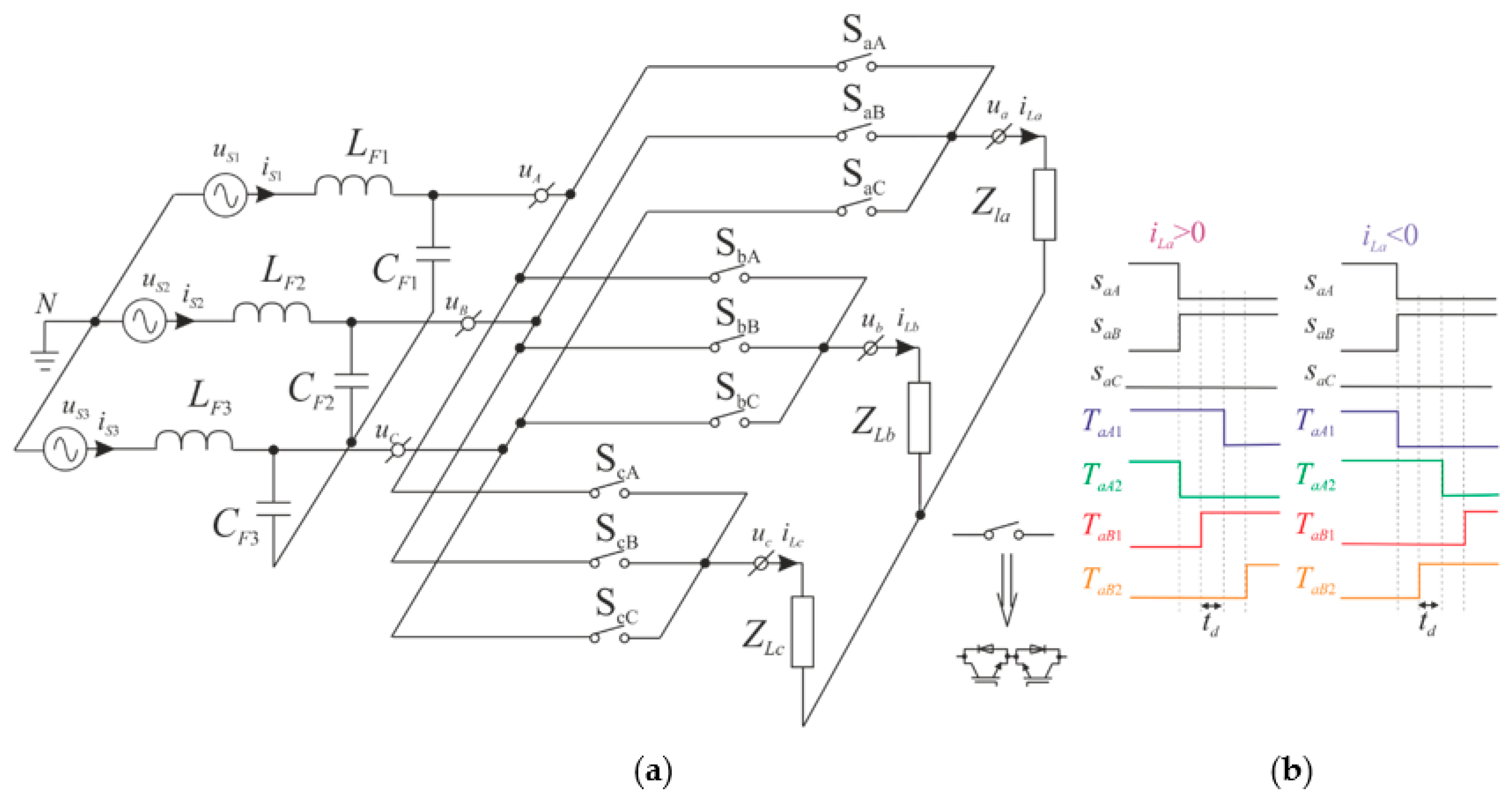
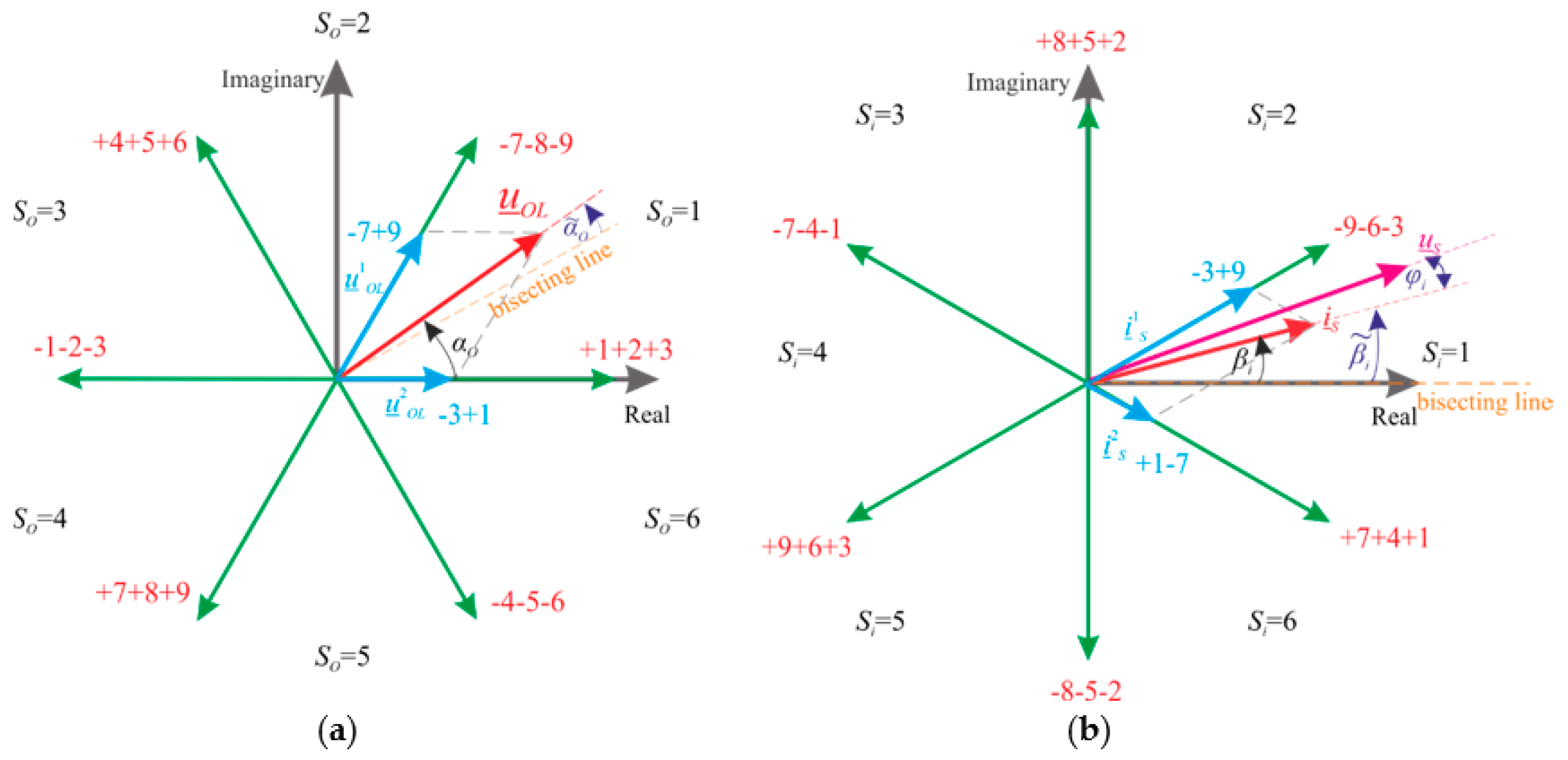
2.2. Matrix Converter with Space Vector Modulation Algorithm

Matrix converters are nowadays an inseparable element of up-to-date power systems. Modern power electronic converters operate in a pulse mode. Due to the nature of voltage of most electric sources, voltages are most often switched, modulating the instantaneous current value. For the switching of voltage and current signals in power electronics systems, power transistors are used. The most commonly used power transistor technology is the insulated gate bipolar transistor (IGBT) made using silicon (Si) technology. This technology enables work with switching frequencies of several dozen kilohertz. In recent years, transistor technologies have emerged that enable a significant increase in the switching frequency to hundreds of kilohertz. These are transistors based on silicon carbide (SiC) [54] and gallium nitride (GaN) [55] technologies. By increasing the switching frequency, it is possible to reduce the size and weight of the converter, especially the passive elements used, such as reactors and capacitors in passive filter systems.
Power electronic converters transform DC and AC electric energy of various values, shapes and frequencies into DC or AC signals of any selected parameters. There is a very large number of different types of power converter from simple designs with one switched transistor to very complex ones with dozens of switching transistors and with various control modulation strategies [56]. Management of power electronic converters with a large amount of transistors and a high switching frequency requires the use of a special control system with high computing power and a large number of pulse-width modulation (PWM) outputs or freely programmable I/O pins. This requirement can be fulfilled by both digital signal processors (DSPs), as well as reconfigurable logic devices such as field programmable gate arrays (FPGAs) [57,58].
The concept of the matrix converter was created in the 1980s and is being constantly developed in the direction of creating new topologies, control algorithms and industrial implementations. The original solution of the direct matrix converter is the topology shown in Figure 1a [59,60,61,62]. Nine power electronics bi-directional switches are connected between the power supply terminals and the load. The most commonly used power switches were made of silicon technology (Si). However, nowadays the application of power switches structured of silicon carbide (SiC) technology is more often considered. Examples of bi-directional switch structures in SiC technology are depicted in Figure 2. The most capable SiC switches are the normally-off common drain anti-paralleled SiC JFET, common source anti-paralleled SiC MOSFET and common emitter anti-paralleled SiC BJTs [63,64]. The use of SiC transistors enables a large increase in the efficiency of converters with high switching frequencies (several dozen kHz) and minimising the dimension of the converter.
The matrix converter directly converts the AC voltage of given parameters into AC voltage with selected parameters, according to the following relations between input and output [59]:
[ v a ( t ) v b ( t ) v c ( t ) ] = [ s a A s a B s a C s b A s b B s c B s c A s c B s c C ] [ v A ( t ) v B ( t ) v C ( t ) ] [ i A ( t ) i B ( t ) i C ( t ) ] = [ s a A s b A s c A s a B s b B s c B s a C s b C s c C ] [ i a ( t ) i b ( t ) i c ( t ) ]
v a b c ( t ) = D ( t ) v A B C i A B C ( t ) = D T i a b c ( t )
The D matrix defining the relationship between input and output voltages is determined on the basis of the adopted modulation strategy. Different modulation strategies have been previously described in the scientific publications [62] and the most well-known are Venturini, scalar, space vector modulation (SVM) and predictive control. The SVM algorithm is commonly used in MC applications. However, in recent times predictive methods have been increasingly implemented. The SVM in the MC control is based on the instantaneous space vector depiction of the MC’s voltage (Equation (3)) end current signals (Equation (4)) in a complex reference system [65].
u _ O L = 2 3 ( u a b ( t ) + e j 2 π 3 u b c ( t ) + e j 2 π 3 u c a ( t ) ) = | u O L | e j α O ( t )
i _ S = 2 3 ( i A ( t ) + e j 2 π 3 i B ( t ) + e j 2 π 3 i C ( t ) ) = | i S | e j β i ( t )
The SVM technique uses so-called “active configurations” and “zero configurations” of power electronics switches, which are listed in the left part of Table 1 and Figure 3. The switching sequence in period TSeq depends on the location of the voltage and current vectors and contains four “active configurations” and one “zero configuration”. The right part of Table 1 determines the switching order depending on the voltage and current sector numbers [65].
The synthesis process of set output voltage uOL space vectors according to Figure 3a is defined as follows:
u _ O L = u _ O L 1 + u _ O L 2 = d I u _ I + d I I u _ I I + d I I I   u _ I I I + d I V u _ I V
where d j = t j T S e q ,   j =   I , I I , I I I , I V , and d 0 = 1 d I d I I d I I I   d I V . The dj coefficients are defined as the relative switch-on times of individual switch configurations and are calculated from the following formulas:
d I = ( 1 ) S O + S i + 1 2 q c o s (   α ˜ O π 3 ) c o s (   β ˜ i π 3 ) 3 c o s φ i ,
d I I = ( 1 ) S O + S i 2 q c o s (   α ˜ O π 3 ) c o s (   β ˜ i + π 3 ) 3 c o s φ i ,
d I I I = ( 1 ) S O + S i 2 q c o s (   α ˜ O + π 3 ) c o s (   β ˜ i π 3 ) 3 c o s φ i ,
d I V = ( 1 ) S O + S i + 1 2 q c o s (   α ˜ O + π 3 ) c o s (   β ˜ i + π 3 ) 3 c o s φ i .
The angles α ˜ O and β ˜ i are designated relative to the bisecting line of each segment (So and Si) of the complex coordinate system and set voltage and current space vectors, respectively. For such definition, these angles are limited by the following ranges: π 6 <   α ˜ O < π 6 ;   π 6 <   β ˜ i < π 6 . The MC voltage gain is controlled by q factor. The maximum value of q is equal 3 2 0.866 .
The second algorithm necessary for correct operation of the MC is the commutation algorithm of the transistors. Few commutation approaches have been described in the literature [66] and the most often used is the four-step commutation algorithm. In this approach, the way of current flow over the commutation switches must be controlled, since the switching sequence depends on the direction of the current as is shown in Figure 1b. An identical switching arrangement happens between any transistors in two bidirectional switches in individually output phase.

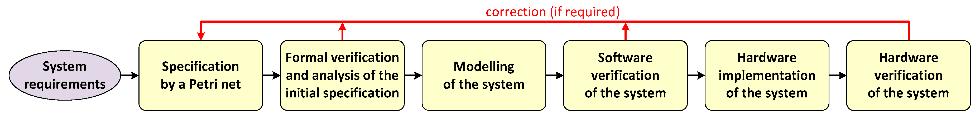
3. The Idea of the Proposed Method

The proposed design idea consists of six main steps. The presented technique is heavily focused on the verification aspects. Therefore, the system is checked three times: at the specification stage (formal verification methods), after the modelling stage (software verification), and finally after the implementation in a programmable device (hardware verification).
In more detail, the proposed design technique of cyber-physical systems contains the following steps (Figure 4):
  • Specification of the CPS by a safe and live Petri net (based on the system requirements);
  • Formal verification and analysis of the initial specification;
  • Modelling of the system;
  • Software verification of the system;
  • Hardware implementation of the system with the application of the programmable device;
  • Hardware verification of the system.
Let us describe each of the stages of the proposed method in more detail.

3.1. Specification of the CPS by a Petri Net

Initially, based on the informal system requirements, a CPS is specified by a Petri net. Such a description naturally reveals the concurrency relations in the system. Furthermore, Petri nets are supported by various verification techniques that permit the detection of errors and mistakes at an early specification stage. Therefore, they can be found in various fields, like flexible manufacturing systems [25,67], system engineering [68], distributed systems [26], robot-control applications [69], transportation [70], as well as systems implemented in digital devices [49,51,71].

3.2. Formal Verification and Analysis of the Initial Specification

Formal verification of a Petri net ensures that initial requirements are satisfied in the finally implemented system. The specification of the control part of the CPS can be formally verified with the application of the model checking technique [72,73]. Such a formal verification can be automatically performed by the so-called model checkers, e.g., the nuXmv tool [74]. The verifiable models (in the format of the chosen model checker) are quite long, so they can be automatically generated based on the much shorter specification models.
In the paper, we propose to use the simple rule-based logical model (RBLM) (based on the Petri net model) to perform the stage of model checking of the CPS specification. The RBLM describes places and transitions (basic elements of a net) and presents how the marking evolves. Note that the proposed design approach allows for application of any known model-checking tools. In our considerations, we use the nuXmv symbolic model checker, supported by m2vs tool ([26]).
The m2vs tool, based on the RBLM, generates a verifiable model, but additionally also a synthesizable model of the analysed system [26]. It is worth noting, that the complete process is automated. As a result, two models of the CPS are obtained. The first one includes a specification in a synthesizable VHDL code (and can be used for prototype implementation), and the second one contains a verifiable model (in the format of the nuXmv tool), which has only to be supplemented by the requirements definition to perform the model checking process. Both models reflect the primary, Petri net-based specification and are consistent with each other.
Beside the methods, additional analysis of the system is performed. Firstly, safeness of the net is checked. It can be executed, for example, by computation of SM-cover in the net [75,76]. Furthermore, main properties of the net can be checked [26,49,51,52,53,77,78,79,80,81,82,83,84,85], such as classification of the net, number of reachable states, number of place invariants, total number of SMCs, etc. Additionally, concurrency, as well as sequentiality relations in the net can be examined [23]. It should be noted that all the above properties can be easily analysed automatically within dedicated tools, such as IOPT-Tools [86], PIPE [87] or Hippo system [88].

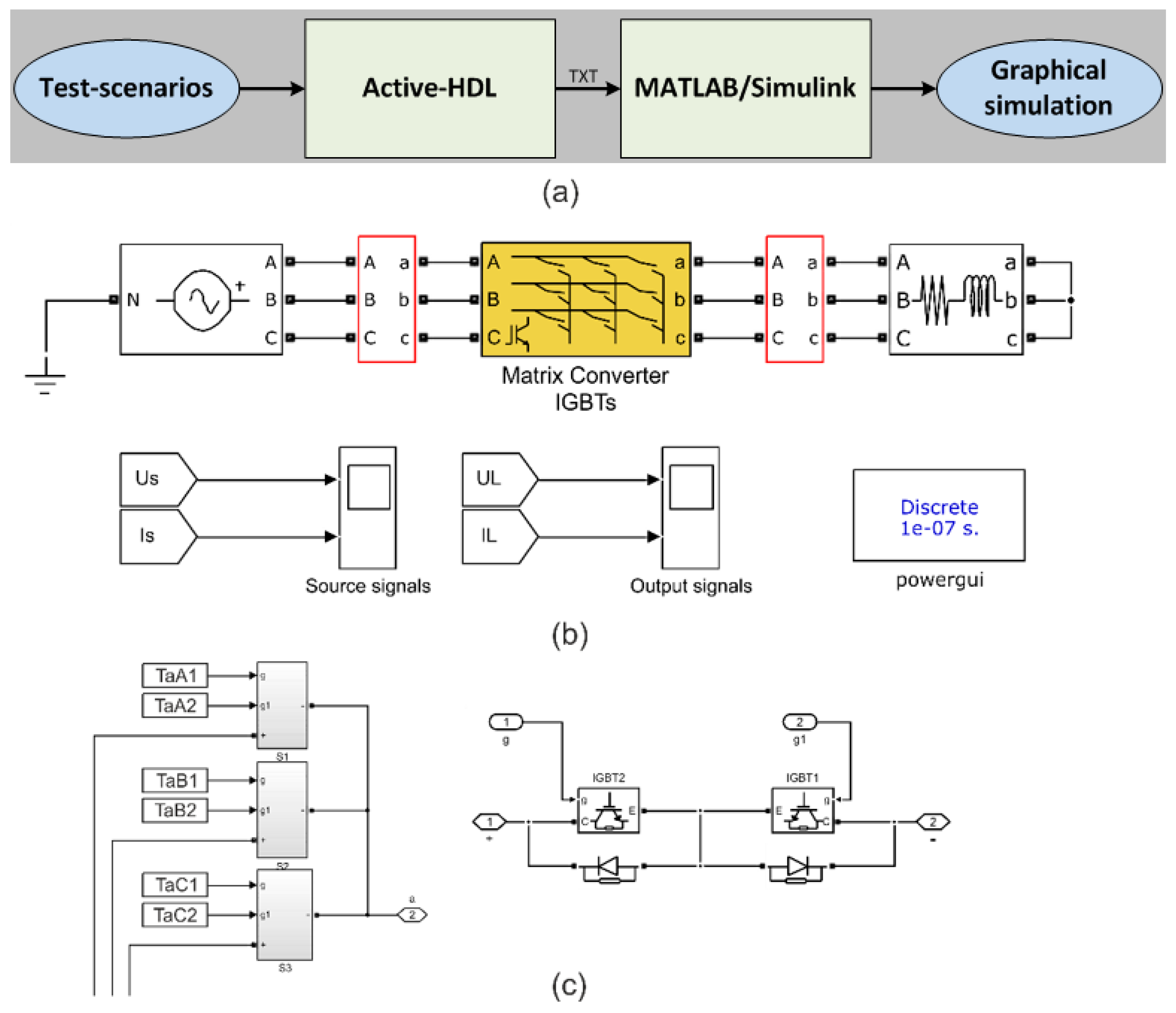
3.3. Modelling of the System

In the proposed design method, after successful formal verification and analysis of the initial specification, the system is modelled with hardware description language (HDL). The system is divided into some components (modules) that are connected with each other via internal buses. The modules can be executed either sequentially or concurrently, which show how the tasks are realised within the system. The components, which are synchronous, additionally use the clock signal. Detailed information about modelling of the system in HDLs can be found in other authors publications ([26,49,89,90], please also refer to Section 4.3, where modelling of exemplary CPS is shown). Note that there is no restriction regarding the applied hardware description language. In the proposed approach, the CPS can be modelled in any language that is oriented for further implementation in hardware. In particular, this paper shows use of Verilog code (as shown in Section 4.3), but VHDL language (or even mixed design—based on both, Verilog and VHDL) can be applied, as well.

3.4. Software Verification of the System

The correct functionality of the designed algorithms can be checked using dedicated simulation programs by performing the so-called numeric experiment. In order to perform such verification, all signals should be implemented in the form of numerical data (test-scenario) in a simulation system. In the presented design flow, a MATLAB simulation is applied. This tool (delivered by MathWorks) offers versatile and robust options in simulation and control verification of power electronic converters using Simulink Toolbox from MathWorks. It is assumed that the initial data is stored in a text file, which is the result of software simulation of HDL code. This simulation can be performed with the use of any tool that supports verification of the HDL code (such as Active-HDL from Aldec, ModelSim from Mentor Graphics, etc.). In this paper, we shall apply Active-HDL simulator to produce software simulation, which will be further used for numerical testing of the correctness of the prototyped SVM algorithm (Section 4.4).

3.5. Hardware Implementation of the System with the Application of the Programmable Device

After software verification, the system can be physically implemented in hardware with the application of the programmable device. The implementation involves additional operations, such as logic synthesis, logic implementation and generation of the final bit-stream (data sent in order to program an FPGA). Particular actions are performed as required by the vendor of the targeted device using the specialised tools. In this paper, we follow the guidelines from Xilinx, since the algorithm presented the case-study example was implemented in the FPGA produced by this vendor. Note that more detailed information about implementation of systems specified by Petri nets in FPGAs can be found in [89].

3.6. Hardware Verification

Finally, the correctness of the algorithm (implemented in hardware in the previous stage) is verified by performing test-scenarios and measuring the control signals. In the paper it is proposed to apply the verification based on the measurement by the oscilloscope, which is directly connected to a device (FPGA, see Section 4.6). It is worth noting, that the test-scenarios can be the same as in the software verification step. Only by obtaining correct software and hardware verification results can there be any confidence that the designed and implemented system meets all the initial requirements.

4. Case-Study Example (Hardware Implementation of the Proposed Method)

Let us explain the approach proposed in the paper with the use of a real cyber-physical system. As an exemplary CPS, a direct matrix converter with space vector modulation algorithm (described in detail in Section 2.2) was chosen. The SVM algorithm was initially specified with the use of a live and safe Petri net. Then, it was analysed and formally verified to ensure that the specification does not contain any ill-modelled parts. At the subsequent step, the system is modelled with the use of HDL. Before the implementation in the hardware, the system was once again verified (based on the description in the HDL code). Finally, after the hardware implementation, the CPS was verified for the third time to be sure that the realised system meets all the initial requirements. Let us describe each of the steps in more detail.

4.1. Specification of the System with the Use of a Petri Net

Initially, based on the system requirements, a Petri net is created (Figure 5). The net is live and safe (Definitions 3 and 4 presented in Section 2.1). The net contains 49 places and 31 transitions. 32 places (marked in Figure 5 in blue) are associated with particular hardware tasks executed by the system. The remaining 17 places (marked in yellow) are used for synchronisation purposes. It is worth mentioning that hardware tasks (marked in blue) could be performed sequentially or concurrently. To perform the SVM algorithm, the 32 main “cyber” tasks have to be realised. Most of them are executed concurrently, e.g., commutation signal generation or computations of values for load voltages and source currents.
The presented system works as follows. The realisation of the SVM algorithm starts from the place p 1 (the initial marking of the net). Then, based on the input values, the instantaneous values of the load voltages u a b , u b c , u c a (places p 2 , p 3 , and p 4 ) and source currents i A , i B , i C (places p 5 , p 6 , and p 7 ) are set. Next, the real and imaginary parts for the space vectors u _ O L and i _ S are concurrently computed [91]. The place p 16 is assigned with the computation of the real part (Re) of the space vector for u _ O L :
R e ( u _ O L ) = 1 3   ( 2 u a b u b c u c a   )
while place p 17 is in response for the imaginary part (Im) of the space vector for u _ O L computation:
I m ( u _ O L ) = 3 3   ( u b c u c a ) .
In an analogous way, the calculation of the real part (Re) of the space vector for i _ S (place p 18 ) is performed:
R e ( i _ S ) = 1 3   ( 2 i A i B i C )
and place p 19 is assigned with the calculation of the imaginary part (Im) of the space vector for i _ S :
I m ( i _ S ) = 3 3   ( i B i C ) .
Afterwards, computations regarding sectors and angles are executed (concurrently for voltages and currents). Places p 20 , p 22 , and p 24 are responsible for the computation of angle α ˜ O for u _ O L , the sector S O computation and angle α O scaling, respectively.
In the place p 20 the angle α O among the real and imaginary parts of the space vector for u _ O L is calculated according to the equation:
α O = a t g I m ( u _ O L ) R e ( u _ O L ) .
Then, based on the angle α O the calculation of the sector S O for the voltage space vector is computed (place p 22 ). Finally, in place p 24 scaling (normalisation) of the angle α O from the range π α O π to the range π 6   α ˜ O ( π 6 ) is performed depending on the sector S O [91].
Simultaneously to the places p 20 , p 22 , and p 24 , the calculation of angle β ˜ i for i _ S , the sector S i and angle β   ˜ i scaling is performed (places p 21 , p 23 , and p 25 ).
Similarly, the computation of the angle β i among the real and imaginary parts of the space vector for i _ S (place p 21 ) is executed:
β i = a t g I m ( i _ S ) R e ( i _ S ) .
Based on the angle β i (place p 23 ), the sector S i for the voltage space vector is computed. Lastly, according to the place p 25 the angle β i is scaled from the initial range π β i π to the range π 6 β ˜ i π 6 .
Places p 26 , , p 29 are responsible for data transformation, and places p 30 , , p 33 perform the computation of the trigonometric functions. Then, the modulation duty cycles (within concurrent places p 42 , , p 45 ) are computed. Based on those results, the internal PWM signals S a A , , S c C are computed (place p 46 ).
Finally, the output commutation signals (TaA1, TaA2, TaB1, TaB2, TaC1, TaC2, TbA1, TbA2, TbB1, TbB2, TbC1, TbC2, TcA1, TcA2, TcB1, TcB2, TcC1, TaC2) are generated—each line independently (place p 47 for line a, place p 48 for line b, and p 49 for line c).

4.2. Formal Verification and Analysis of the Initial Specification

The net from Figure 5 can be formally verified using the model checking technique and the simple rule-based logical model (RBLM). In order to do this, the net is firstly written as an RBLM, where the only variables are Petri net places. The initialisation therefore includes only the initial marking of the net, i.e., place p 1 . Then, all the transitions from the Petri net are written as separate rules, each one consisting of pre-conditions (conditions for firing a transition) and post-conditions (showing how the net marking changes in the next state of the system). The rules for the considered case study are listed in Listing 1. Please note, that each rule is labelled, and the post-conditions include both places that become inactive (do not include a token anymore, indicated by exclamation mark) and places that become active (already have a token).
Listing 1. Rules in the rule-based logic model (RBLM) of the Petri net from Figure 5.
TRANSITIONS
t1: p1 -> X (!p1 & p2 & p3 & p4 & p5 & p6 & p7);
t2: p3 -> X (!p3 & p8 & p10);
t3: p4 -> X (!p4 & p9 & p11);
t4: p5 -> X (!p5 & p12 & p14);
t5: p6 -> X (!p6 & p13 & p15);
t6: p2 & p8 & p9 -> X (!p2 & !p8 & !p9 & p16);
t7: p10 & p11 -> X (!p10 & !p11 & p17);
t8: p12 & p13 -> X (!p12 & !p13 & p18);
t9: p7 & p14 & p15 -> X (!p7 & !p14 & !p15 & p19);
t10: p16 & p17 -> X (!p16 & !p17 & p20);
t11: p18 & p19 -> X (!p18 & !p19 & p21);
t12: p20 -> X (!p20 & p22);
t13: p21 -> X (!p21 & p23);
t14: p22 -> X (!p22 & p24);
t15: p23 -> X (!p23 & p25);
t16: p24 & p25 -> X (!p24 & !p25 & p26 & p27 & p28 & p29);
t17: p26 -> X (!p26 & p30);
t18: p27 -> X (!p27 & p31);
t19: p28 -> X (!p28 & p32);
t20: p29 -> X (!p29 & p33);
t21: p30 -> X (!p30 & p34 & p38);
t22: p31 -> X (!p31 & p36 & p40);
t23: p32 -> X (!p32 & p35 & p37);
t24: p33 -> X (!p33 & p39 & p41);
t25: p34 & p35 -> X (!p34 & !p35 & p42);
t26: p36 & p37 -> X (!p36 & !p37 & p43);
t27: p38 & p39 -> X (!p38 & !p39 & p44);
t28: p40 & p41 -> X (!p40 & !p41 & p45);
t29: p42 & p43 & p44 & p45 -> X (!p42 & !p43 & !p44 & !p45 & p46);
t30: p46 -> X (!p46 & p47 & p48 & p49);
t31: p47 & p48 & p49 -> X (!p47 & !p48 & !p49 & p1);
The complete RBLM for the case study consists of 36 lines. Then, the developed m2vs tool is used to automatically generate the verifiable model in the nuXmv format, but also the synthesizable prototype model in the VHDL language. The verifiable model consists of 345 lines, which is almost ten times more than the initial RBLM, but which is needed to perform formal verification. The synthesizable model consists of 229 lines, which is still over six times more than the RBLM. Let us point out that thanks to the automatic generation of models, both resulting models are consistent with each other, and the prototype implementation in the FPGA device satisfies the requirements that hold in the verifiable model. The verifiable model has then been supplemented with the list of structural requirements for the modelled system. Model checking of the specification confirms that all places of the net are reachable and that the Petri net is live.
After formal verification step, the initial specification expressed as a Petri net model was analysed with the application of dedicated on-line tools: Hippo system [88] and the IOPT-Tools [86]. The following properties of the Petri net were checked by these tools: classification of the net, safeness, liveness, number of reachable markings (states in the net), the minimal number of SMCs that are required to cover the net. Table 2 presents the achieved results of analysis.
Regarding the presented results, it can be noticed that two crucial properties of the Petri net have been met—the analysed net is safe and live. This means that the designed system neither contains any deadlocks, nor unreachable states. Therefore, it is specified in a proper way.
The detailed analysis of the Petri net shows that the net belongs to the MG-nets. This information is very useful if further optimisations are planned, because this particular subclass has interesting properties [49,52]. Furthermore, the total number of p-invariants in the Petri net is equal to 240, while the number of reachable markings (states) is 239. Moreover, the net is SM-coverable, which indicates that the system can be decomposed into independent components. This can be useful in the case of the system implementation in devices that operate in a sequential manner (such as programmable logic controllers, PLCs) or if further dynamic partial reconfiguration of the system in FPGA devices is planned (see [48] for details).
To conclude the above discussion, the results of the analysis of the initial specification show that the net is safe, live and has been properly designed. Furthermore, it is possible to apply further optimisations of the specified system.

4.3. Modelling of the System
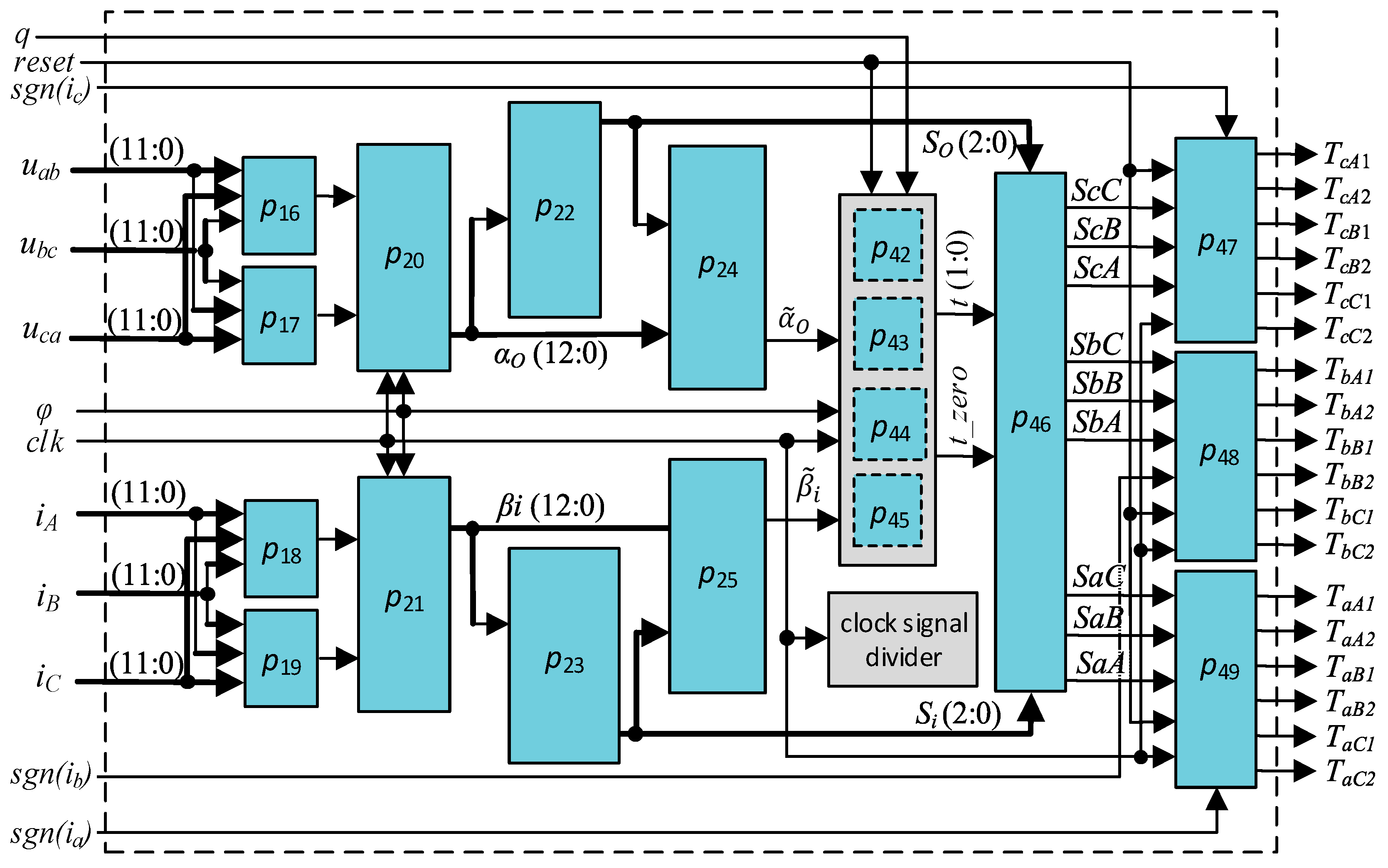
Once the designer is sure that the initial specification does not contain any formal errors, nor mistakes, the system can be modelled with the application of the HDL. It is a non-trivial task because many of the places in the designed Petri net relate to a quite complicated computation task (especially if the hardware has limited hardware resources). In the proposed approach the Verilog language was chosen as a modelling language.
Figure 6 presents the diagram of the modelled system based on the Petri net. Each place of the Petri net in Figure 5 marked in blue refers to the particular module of the system. All these modules are connected to each other via internal buses. Moreover, the clock signal (clk) was introduced to the system because most of components are synchronous. Furthermore, to reset seven blocks of the system the special ‘reset’ signal was delivered.
Each of the 19 modules presented in Figure 6 is responsible for a computational task:
  • four modules ( p 16 , …, p 19 ) are responsible for calculation of the real and imaginary parts of the space vector for voltages and currents;
  • two modules ( p 20 , p 21 ) perform angle computation of the space vectors;
  • two modules ( p 22 , p 23 ) compute sectors of the space vectors;
  • two modules ( p 24 , p 25 ) realise angle normalisation;
  • four modules ( p 42 , …, p 45 ) execute duty computation and organisation;
  • one module ( p 46 ) is responsible for switching of the PWM signals;
  • three modules ( p 47 , …, p 49 ) generate final commutation signals;
  • one module was designed for clock signal (clk) division.
It is worth noting, that many of the above described modules are executed concurrently (for example four modules that calculate the real or imaginary parts of the space vectors, two modules responsible for angle normalisation, or three modules generating final commutation signals). Moreover, the computation of the mathematical arctangent function is realised with the application of a coordinate rotation digital computer (CORDIC) method. In particular, the intellectual property (IP-core) from Xilinx is used [92].
The exemplary Verilog specification of selected module ( p 16 —calculation of the real part of the space vector for voltages) is presented in Listing 2. The same module is used in block p 18 , however different input is delivered for this module instance. The internal blocks Multiply_1QN simply perform multiplication of remaining values in the remaining notation 1QN [92].
Listing 2. Verilog source code of the real part computation for the space vector for voltages ( p 16 ,   p 18 ).
//computation of Re: result=2/3*x1-1/3*x2-1/3*x3
module Calculate_Re(result,x1,x2,x3);
    output [12:0] result;
    input [12:0] x1,x2,x3;
    wire signed [12:0] x1_signed,x2_signed,x3_signed;
    Multiply_1QN m1 (x1_signed,x1,13’b 0001010101010); //2/3 * x1
    Multiply_1QN m2 (x2_signed,x2,13’b 0001010101010); //1/3 * x2
    Multiply_1QN m3 (x3_signed,x3,13’b 0001010101010); //1/3 * x3
    wire signed [12:0] Re_signed;
    wire [12:0] Re;
    assign Re_signed=x1_signed+x1_signed-x2_signed-x3_signed;
         assign Re=(Re_signed [12:11]==2’b10)?13’b1100000000000:
                 (Re_signed [1 2:11]==2’b01)?13’b0100000000000:Re_signed;
    assign result=Re;
endmodule
              

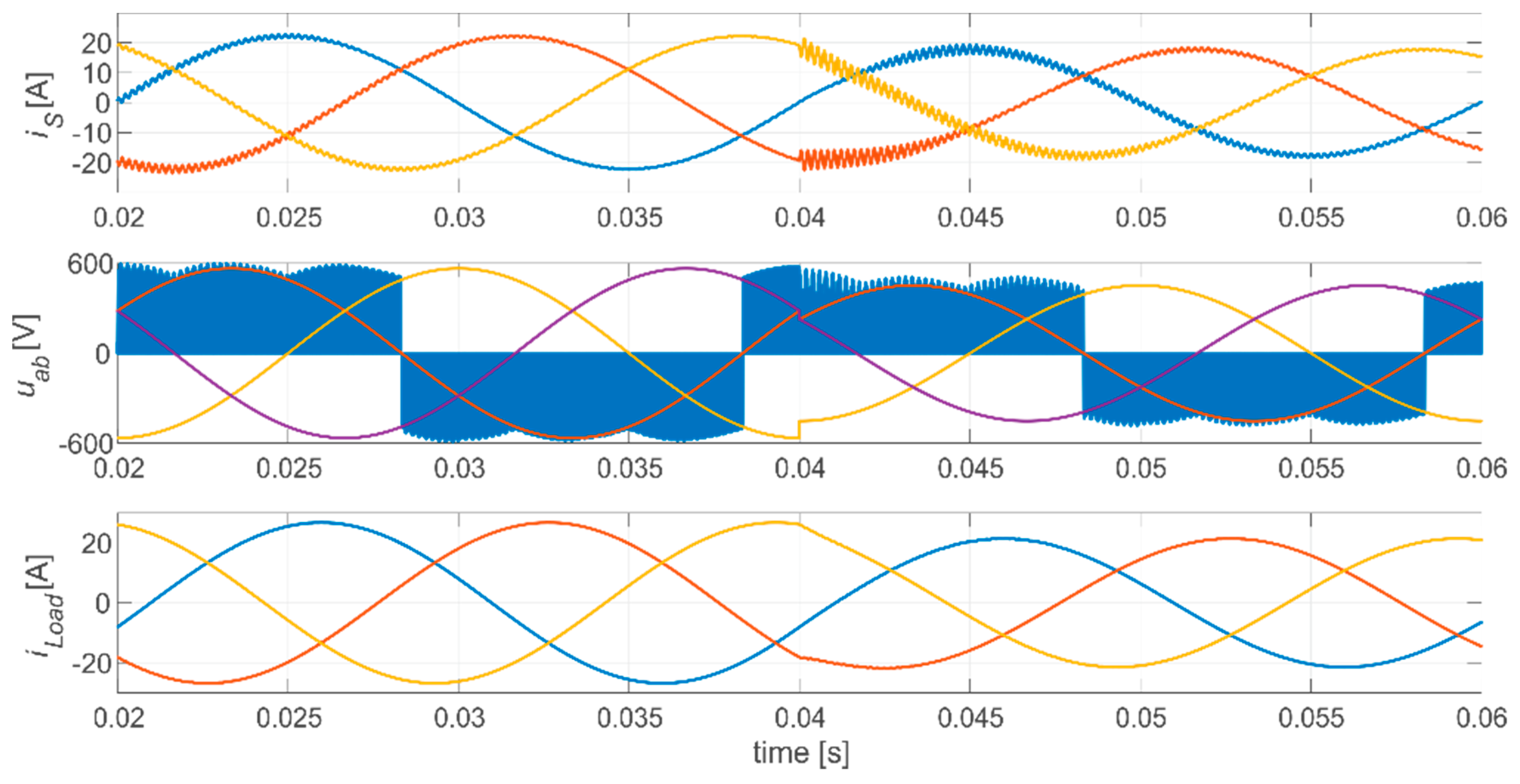
4.4. Software Verification of the System

Figure 7a presents the procedure of the software verification of the system. The verification process applied two specialised tools.
Firstly, based on the test-scenarios prepared by the designer, Active-HDL software from Aldec was used in order to generate results in text format. Those values were further read into the MATLAB/Simulink tool from MathWorks. The main view of Simulink program is presented in Figure 7b. A program presenting power electronics switches and a part of the program responsible for reading control signals from previously generated files is shown in Figure 7c.
The proper functionality of the SVM modulation algorithm and commutation strategies has been verified. In the obtained results (Figure 8), there were no visible abnormal states resulting from the incorrectness of the created algorithms. Even the disturbance generated in the supply voltage does not cause incorrect results. The obtained output currents without overcurrent change to a steady state point resulting from power supply and load conditions.

4.5. Hardware Implementation of the System

The designed and verified system was modelled with application of the HDL. Then the Verilog specification (using specialised Vivado synthesis tool from Xilinx) was logically synthesised in order to program an FPGA device (XC7A35T from Xilinx Artix-7 family was used). The consumption of the hardware resources of XC7A35T device is presented in Table 3.
The results show that the consumption of the hardware resources in each case was below 40%. This means that also other components can be integrated in the system (e.g., analogue-to-digital converters, specialised IP-cores).
After the synthesis of the system, using bit-stream generated at this stage, the implementation of the real hardware device was done. To realise this task, the Basys 3 Artix-7 FPGA Trainer Board from Digilent with integrated XC7A35T-1CPG236C Xilinx FPGA device was used. The values of the prerequisites were as follows:
  • the sequence of modulation period was set to 100 kHz (the value of T S e q was set to 10 μs);
  • the commutation switch period was set to 0.2 μs;
  • the value of the parameter ϕ i (used in Equations (6)–(9)) was set to 0 (constant value);
  • the main oscillator (clock signal) frequency was set to 100 MHz.

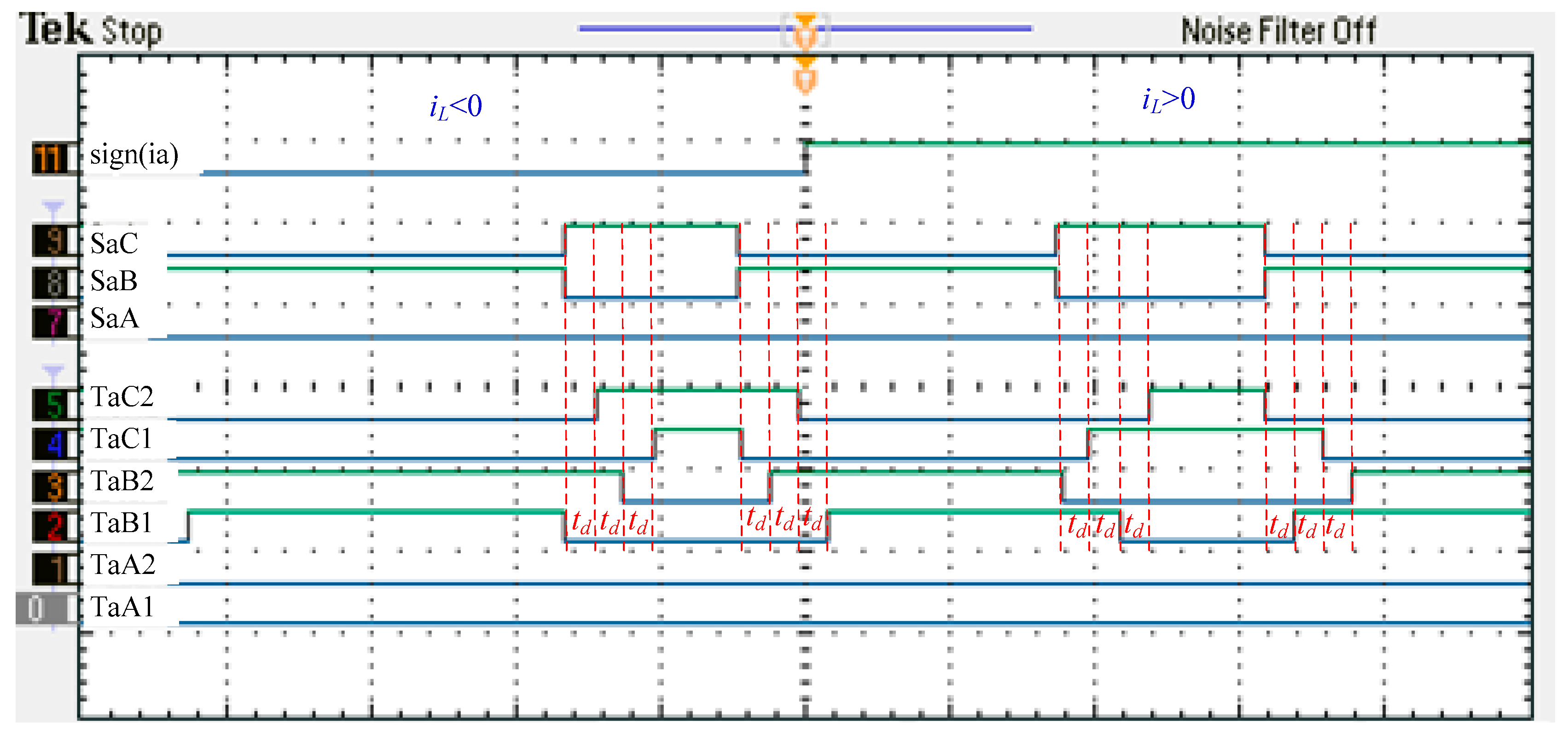
4.6. Hardware Verification of the System

Lastly, the appropriate behaviour of the implemented algorithm was verified by measuring the transistor control signals direct on the I/O pins of the FPGA device. Figure 9 shows the empirical results of measurement signals. The S a A , S a B , S a C signals obtained during SVM process, as well as the individual transistors T a A 1 , T a A 2 , T a B 1 , T a B 2 , T a C 1 , T a C 2 signals obtained during the commutation strategy and the current direction signal s i g n ( i a ) , are shown in the presented oscillogram. The different switching arrangements of transistors occur for different sign of the load current. For the negative current sign, the SaB is in turn-on and the SaA is in turn-off. The arrangement is as follows: TaA1→OFF, TaB2→ON, TaA2→OFF, TaB1→ON. For the opposite current sign, the SaC is in turn-on and the SaB is in turn-off. The sequence is as follows: TaB2→OFF, TaC1→ON, TaB1→OFF, TaC2→ON. The delay time (td) of the transistors’ switching time is equal to 0.2 μs. The presented signals agree to the general switching pattern which is shown in Figure 1b. The presented testing procedure gives high hopes that the implementation of the obtained algorithms in the real prototype will not damage it and will ensure its correct operation.

5. Conclusions

A novel prototyping method of a control part of a cyber-physical system is proposed in the paper. The presented solution is aimed at the verification of the designed system, and thus it bridges the gap in current CPS design methods. The approach is strongly focused on the verification aspects. Indeed, the system is analysed and verified three times at various stages of the design flow. Firstly, the model checking of the initial specification is executed and the system is verified against the structural properties which permits to avoid formal errors and prototyping mistakes (such as deadlocks or non-reachable states). Afterwards, the CPS is verified at the software modelling stage (software simulation and numerical verification). Finally, hardware verification of the already implemented CPS is performed.
The main advantage of the proposed verification-oriented methodology relies on the multiple verification of the system. The CPS is checked at various stages of the design process in order to minimise the possible errors and mistakes. It is worth noting that the presented solution does not involve any dedicated tools (except MATLAB/Simulink software), nor additional conversions. It means that the designer is able to perform the formal verification with the application of any known tool that supports model-checking of Petri nets (in the paper nuXmv model checker was applied). Moreover, the software verification can be executed with the use of any simulator (in the paper Active-HDL was applied). Finally, there are no restrictions regarding the modelling stage. The system can be modelled in any hardware language that is designed for further implementation in programmable devices. In the paper, Verilog was used, however VHDL language can be equally applied (to describe the whole design or particular modules).
The main limitation of the proposed design methodology refers to the specification stage. The system ought to be described by a Petri net. Obviously, it requires specialised knowledge on the designer’s side. Furthermore, the proposed technique applies dedicated MATLAB/Simulink software. This step (software verification) is not necessary in the design process, but it gives a high degree of assurance of proper functionality of the system before the implementation in hardware.
For future research, it is planned to enhance the proposed technique by other specification methods of CPS. In particular, other graphical descriptions based on the UML-like state machine diagrams are going to be considered. These diagrams support the two important features of the nowadays designed CPS-like hierarchy and concurrency and are very intuitive and efficient (especially in combination with MDD techniques).
Furthermore, the proposed verification-oriented design approach, where the designed CPS is analysed and verified several times, can be also very useful in the safety-critical control systems development process, which is highly focused on the validation and verification aspects.
Moreover, other software verification methods will be analysed to propose alternatives for MATLAB/Simulink. Although the fact is that this tool is very popular among engineers, there are still to be found some designers that are not closely familiar with this software. Another reason is that the MATLAB/Simulink system is quite expensive and under certain circumstances can be substituted by open source alternatives.

Author Contributions

Conceptualization, R.W., G.B., P.S. and I.G; methodology, R.W., G.B. and P.S.; software, R.W., G.B. and P.S.; validation, R.W., G.B., P.S., I.G. and M.W.; formal analysis, I.G. and M.W.; investigation, R.W., G.B. and P.S.; writing—original draft preparation, R.W., G.B., P.S., I.G. and M.W.; writing—review and editing, G.B.; supervision and project administration, R.W.; funding acquisition, R.W., G.B. and P.S.

Funding

This research was partially done as a result of an internship of the author (R. Wisniewski) at the University of California, Berkeley. The internship was financed by Polish National Science Centre under Grant No. 2018/02/X/ST6/01861. The APC was founded by R. Wisniewski, G. Bazydlo and P. Szczesniak.

Conflicts of Interest

The authors declare no conflict of interest.

References

  1. Lee, E.A.; Seshia, S.A. Introduction to Embedded Systems, A Cyber-Physical Systems Approach, 2nd ed.; print. 1.08.; LeeSeshia.org: Lulu, CO, USA, 2017; ISBN 9780557708574. [Google Scholar]
  2. Yu, Z.; Zhou, L.; Ma, Z.; El-Meligy, M.A. Trustworthiness modeling and analysis of cyber-physical manufacturing systems. IEEE Access 2017, 5, 26076–26085. [Google Scholar] [CrossRef]
  3. Karatkevich, A. Dynamic Analysis of Petri Net-Based Discrete Systems; Lecture notes in control and information sciences; Springer: Berlin, Germany, 2007; ISBN 9783540714644. [Google Scholar]
  4. Ali, S.; Balushi, T.A.; Nadir, Z.; Hussain, O.K. Cyber Security for Cyber Physical Systems; Springer International Publishing AG, Springer: Cham, Switzerland, 2018. [Google Scholar]
  5. Dey, N.; Ashour, A.S.; Shi, F.; Fong, S.J.; Tavares, J.M.R.S. Medical cyber-physical systems: A survey. J. Med. Syst. 2018, 42, 74. [Google Scholar] [CrossRef] [PubMed] [Green Version]
  6. Zhang, Y.; Qiu, M.; Tsai, C.-W.; Hassan, M.M.; Alamri, A. Health-CPS: Healthcare cyber-physical system assisted by cloud and big data. IEEE Syst. J. 2017, 11, 88–95. [Google Scholar] [CrossRef]
  7. Shih, C.-S.; Chou, J.-J.; Reijers, N.; Kuo, T.-W. Designing CPS/IoT applications for smart buildings and cities. IET Cyber-Phys. Syst. Theory Appl. 2016, 1, 3–12. [Google Scholar] [CrossRef]
  8. Guo, Y.; Hu, X.; Hu, B.; Cheng, J.; Zhou, M.; Kwok, R.Y.K. Mobile cyber physical systems: Current challenges and future networking applications. IEEE Access 2018, 6, 12360–12368. [Google Scholar] [CrossRef]
  9. Khaitan, S.K.; McCalley, J.D. Cyber physical system approach for design of power grids: A survey. In Proceedings of the 2013 IEEE Power & Energy Society General Meeting, Vancouver, BC, Canada, 25 November 2013; pp. 1–5. [Google Scholar]
  10. Khaitan, S.K.; McCalley, J.D. Design techniques and applications of cyberphysical systems: A survey. IEEE Syst. J. 2015, 9, 350–365. [Google Scholar] [CrossRef]
  11. Hahanov, V. Cyber Physical Computing for IoT-DRIVEN Services; Springer International Publishing AG, Springer: Cham, Switzerland, 2018; ISBN 9783319548258. [Google Scholar]
  12. Huang, D.; Deng, Z.; Wan, S.; Mi, B.; Liu, Y. Identification and prediction of urban traffic congestion via cyber-physical link optimization. IEEE Access 2018, 6, 63268–63278. [Google Scholar] [CrossRef]
  13. Gomes, L.; Barros, J.; Costa, A. Modeling Formalisms for Embedded System Design, Embedded Systems Handbook; Taylor and Francis Group, LLC: London, UK, 2006. [Google Scholar]
  14. Peng, S.S.; Zhou, M.C. Ladder diagram and Petri-net-based discrete event control design methods. IEEE Trans. Syst. Man Cybern. Appl. Rev. 2004, 34, 523–531. [Google Scholar] [CrossRef]
  15. Grobelny, M.; Grobelna, I.; Adamski, M. Hardware behavioural modelling, verification and synthesis with UML 2.x activity diagrams. In Proceedings of the 11th IFAC/IEEE International Conference on Programmable Devices and Embedded Systems—PDeS 2012, Brno, Czech Republic, 23–25 May 2012; pp. 109–114. [Google Scholar]
  16. Goran, F. An Introduction to Hybrid Automata, Numerical Simulation and Reachability Analysis. In Formal Modeling and Verification of Cyber-Physical Systems; Drechsler, R., Kühne, U., Eds.; Springer Vieweg: Wiesbaden, Germany, 2015; pp. 50–81. [Google Scholar]
  17. Zhao, H.; Sun, D.; Yue, H.; Zhao, M.; Cheng, S. Using CSTPNs to model traffic control CPS’. IET Softw. 2017, 11, 116–125. [Google Scholar] [CrossRef]
  18. Fu, Y.; Zhu, J.; Gao, S. CPS information security risk evaluation system based on Petri Net. In Proceedings of the 2017 IEEE Second International Conference on Data Science in Cyberspace (DSC), Shenzhen, China, 26–29 June 2017; pp. 541–548. [Google Scholar]
  19. Gavrilescu, M.; Magureanu, G.; Pescaru, D.; Jian, I. Towards UML software models for cyber physical system applications. In Proceedings of the 20th Telecommunications Forum (TELFOR), Belgrade, Serbia, 20–22 November 2012; pp. 1701–1704. [Google Scholar] [CrossRef]
  20. David, R.; Alla, H. Discrete, Continuous, and Hybrid Petri Nets; Springer: Berlin/Heidelberg, Germany, 2010; ISBN 9783642106682. [Google Scholar]
  21. Reisig, W. Petri Nets: An Introduction; EATCS Monographs on Theoretical Computer Science; Springer: Berlin; Germany, 1985; ISBN 9780387137230. [Google Scholar]
  22. Ye, J.; Zhou, M.; Li, Z.; Al-Ahmari, A. Structural decomposition and decentralized control of petri nets. IEEE Trans. Syst. Man Cybern. Syst. 2018, 48, 1360–1369. [Google Scholar] [CrossRef]
  23. Wisniewski, R.; Wisniewska, M.; Jarnut, M. C-exact hypergraphs in concurrency and sequentiality analyses of cyber-physical systems specified by safe petri nets. IEEE Access 2019, 7, 13510–13522. [Google Scholar] [CrossRef]
  24. Ran, N.; Hao, J.; He, Z.; Seatzu, C. Diagnosability analysis of bounded Petri nets. In Proceedings of the 2018 IEEE 23rd International Conference on Emerging Technologies and Factory Automation (ETFA 2018), Turin, Italy, 4–7 September 2018; pp. 1145–1148. [Google Scholar]
  25. Wu, N.; Zhou, M. System Modeling and Control with Resource-Oriented Petri Nets; Automation and Control Engineering; CRC Press: Boca Raton, FL, USA, 2010; ISBN 9781439808849. [Google Scholar]
  26. Grobelna, I.; Wisniewski, R.; Grobelny, M.; Wisniewska, M. Design and verification of real-life processes with application of petri nets. IEEE Trans. Syst. Man Cybern. Syst. 2017, 47, 2856–2869. [Google Scholar] [CrossRef]
  27. Gruson, F.; Le Moigne, P.; Delarue, P.; Videt, A.; Cimetiere, X.; Arpilliere, M. A simple carrier-based modulation for the SVM of the matrix converter. IEEE Trans. Ind. Inf. 2013, 9, 947–956. [Google Scholar] [CrossRef]
  28. Wang, J.; Song, Y.; Li, W.; Guo, J.; Monti, A. Development of a universal platform for hardware in-the-loop testing of microgrids. IEEE Trans. Ind. Inf. 2014, 10, 2154–2165. [Google Scholar] [CrossRef]
  29. Gan, M.; Wang, S.; Ding, Z.; Zhou, M.; Wu, W. An improved mixed-integer programming method to compute emptiable minimal siphons in S3PR nets. IEEE Trans. Control Syst. Technol. 2018, 26, 2135–2140. [Google Scholar] [CrossRef]
  30. Hehenberger, P.; Vogel-Heuser, B.; Bradley, D.; Eynard, B.; Tomiyama, T.; Achiche, S. Design, modelling, simulation and integration of cyber physical systems: Methods and applications. Comput. Ind. 2016, 82, 273–289. [Google Scholar] [CrossRef] [Green Version]
  31. Lefèvre, J.; Charles, S.; Bosch-Mauchand, M.; Eynard, B.; Padiolleau, E.J. Multidisciplinary modelling and simulation for mechatronic design. Des. Res. (Jdr) 2014, 12, 127–144. [Google Scholar] [CrossRef]
  32. Faruque, M.A.; Canedo, A. Design Automation of Cyber-Physical Systems; Springer International Publishing: Cham, Switzerland, 2019. [Google Scholar]
  33. Kim, K.D.; Kumar, P.R. Cyber–physical systems: A perspective at the centennial. Proc. IEEE 2012, 100, 1287–1308. [Google Scholar]
  34. Quadri, I.R.; Bagnato, A.; Brosse, E.; Sadovykh, A. Modeling methodologies for cyber-physical systems: Research field study on inherent and future challenges. Ada User J. 2015, 36, 246–253. [Google Scholar]
  35. Karsai, G.; Sztipanovits, J. Model-integrated development of cyber-physical systems. In Brinkschulte Software Technologies for Embedded and Ubiquitous Systems; SEUS Lecture Notes in Computer Science, 5287; Springer: Berlin/Heidelberg, Germany, 20008. [Google Scholar]
  36. Kolberg, D.; Berger, C.; Pirvu, B.C.; Franke, M.; Michniewicz, J. CyProF—insights from a framework for designing cyber-physical systems in production environments. Procedia CIRP 2016, 57, 32–37. [Google Scholar] [CrossRef]
  37. Zech, A.; Stetter, R.; Holder, K.; Rudolph, S.; Till, M. Novel approach for a holistic and completely digital represented product development process by using graph-based design languages. Procedia Cirp 2019, 79, 568–573. [Google Scholar] [CrossRef]
  38. Gerostathopoulos, I. Model-Driven Development of Software-Intensive Cyber-Physical Systems. Ph.D. Thesis, Charles University in Prague, Prague, Czechk Republic, 2015. [Google Scholar]
  39. Darragi, N.; Miloudi, E.; Koursi, E.; Collart-Dutilleul, S. Architecture Description Language for Cyber Physical Systems Analysis: A Railway Control System Case Study. In Proceedings of the 14th International conference on Railway Engineering Design and Optimization (COMPRAIL), Rome, Italy, 24–26 June 2014. [Google Scholar]
  40. Drechsler, R.; Kühne, U. Formal Modeling and Verification of Cyber-Physical Systems; Springer Vieweg: Wiesbaden, Germany, 2015. [Google Scholar]
  41. Zheng, X.; Julien, C.; Kim, M.; Khurshid, S. Perceptions on the state of the art in verification and validation in cyber-physical systems. IEEE Syst. J. 2017, 11, 2614–2627. [Google Scholar] [CrossRef]
  42. Sun, Y.; McMillin, B.; Liu, X.; Cape, D. Verifying noninterference in a cyber-physical system the advanced electric power grid. In Proceedings of the Seventh International Conference on Quality Software (QSIC 2007), Portland, OR, USA, 11–12 October 2007; pp. 363–369. [Google Scholar] [CrossRef]
  43. Akella, R.; McMillin, B.M. Model-checking BNDC properties in cyber-physical systems. In Proceedings of the 33rd Annual IEEE International Computer Software and Applications Conference, Seattle, WA, USA, 20–24 July 2009; pp. 660–663. [Google Scholar] [CrossRef]
  44. Automated Technology for Verification and Analysis: 9th International Symposium. In Lecture Notes in Computer Science, Proceedings of the ATVA 2011, Taipei, Taiwan, 11–14 October 2011; Bultan, T.; Hsiung, P.-A. (Eds.) Springer: Berlin/Heidelberg, Germany, 2011; Volume 6996, ISBN 9783642243714. [Google Scholar] [CrossRef]
  45. Bu, L.; Wang, Q.; Chen, X.; Wang, L.; Zhang, T.; Zhao, J.; Li, X. Toward online hybrid systems model checking of cyber-physical systems’ time-bounded short-run behavior. SIGBED Rev. 2011, 8, 7–10. [Google Scholar] [CrossRef]
  46. Thacker, R.A.; Jones, K.R.; Myers, C.J.; Zheng, H. Automatic abstraction for verification of cyber-physical systems. In Proceedings of the 1st ACM/IEEE International Conference on Cyber-Physical Systems—ICCPS ’10; ACM Press: Stockholm, Sweden, 2010; p. 12. [Google Scholar] [CrossRef]
  47. Zheng, X.; Julien, C. Verification and validation in cyber physical systems: Research challenges and a way forward. In Proceedings of the 2015 IEEE/ACM 1st International Workshop on Software Engineering for Smart Cyber-Physical Systems, Florence, Italy, 16–24 May 2015; pp. 15–18. [Google Scholar] [CrossRef]
  48. Wisniewski, R. Dynamic partial reconfiguration of concurrent control systems specified by petri nets and implemented in Xilinx FPGA devices. IEEE Access 2018, 6, 32376–32391. [Google Scholar] [CrossRef]
  49. Wisniewski, R.; Karatkevich, A.; Adamski, M.; Costa, A.; Gomes, L. Prototyping of concurrent control systems with application of Petri Nets and comparability graphs. IEEE Trans. Contr. Syst. Technol. 2018, 26, 575–586. [Google Scholar] [CrossRef]
  50. Martinez, J.; Silva, M. A simple and fast algorithm to obtain all invariants of a generalized Petri net. In Selected Papers from the European Workshop on App. and Theory of Petri Nets, London, UK; Springer: Berlin, Germany, 1982; pp. 301–310. [Google Scholar]
  51. Wisniewski, R.; Bazydlo, G.; Gomes, L.; Costa, A. Dynamic partial reconfiguration of concurrent control systems implemented in FPGA devices. IEEE Trans. Ind. Inf. 2017, 13, 1734–1741. [Google Scholar] [CrossRef]
  52. Murata, T. Petri nets: Properties, analysis and applications. Proc. IEEE 1989, 77, 541–580. [Google Scholar] [CrossRef]
  53. Chen, T.M.; Sanchez-Aarnoutse, J.C.; Buford, J. Petri net modeling of cyber-physical attacks on smart grid. IEEE Trans. Smart Grid 2011, 2, 741–749. [Google Scholar] [CrossRef]
  54. Alves, L.F.S.; Lefranc, P.; Jeannin, P.-O.; Sarrazin, B. Review on SiC-MOSFET devices and associated gate drivers. In Proceedings of the 2018 IEEE International Conference on Industrial Technology (ICIT); IEEE: Lyon, France, 2018; pp. 824–829. [Google Scholar]
  55. Jones, E.A.; Wang, F.F.; Costinett, D. Review of Commercial GaN Power Devices and GaN-Based Converter Design Challenges. IEEE J. Emerg. Sel. Topics Power Electron. 2016, 4, 707–719. [Google Scholar] [CrossRef]
  56. Khomfoi, S.; Tolbert, L.M. Power Electronics Handbook: Devices, Circuits, and Applications Handbook, 4th ed.; Rashid, M.H., Ed.; Elsevier: Burlington, MA, USA, 2017; ISBN 9780123820365. [Google Scholar]
  57. Diao, L.; Tang, J.; Loh, P.C.; Yin, S.; Wang, L.; Liu, Z. An Efficient DSP–FPGA-based implementation of hybrid PWM for electric rail traction induction motor control. IEEE Trans. Power Electron. 2018, 33, 3276–3288. [Google Scholar] [CrossRef]
  58. Hamouda, M.; Blanchette, H.F.; Al-Haddad, K.; Fnaiech, F. An efficient DSP-FPGA-based real-time implementation method of SVM algorithms for an indirect matrix converter. IEEE Trans. Ind. Electron. 2011, 58, 5024–5031. [Google Scholar] [CrossRef]
  59. Andreu, J.; Kortabarria, I.; Ormaetxea, E.; Ibarra, E.; Martin, J.L.; Apinaniz, S. A step forward towards the development of reliable matrix converters. IEEE Trans. Ind. Electron. 2012, 59, 167–183. [Google Scholar] [CrossRef]
  60. Kolar, J.W.; Friedli, T.; Rodriguez, J.; Wheeler, P.W. Review of three-phase PWM AC–AC converter topologies. IEEE Trans. Ind. Electron. 2011, 58, 4988–5006. [Google Scholar] [CrossRef]
  61. Rodriguez, J.; Rivera, M.; Kolar, J.W.; Wheeler, P.W. A review of control and modulation methods for matrix converters. IEEE Trans. Ind. Electron. 2012, 59, 58–70. [Google Scholar] [CrossRef]
  62. Szczesniak, P. Challenges and design requirements for industrial applications of AC/AC power converters without DC-link. Energies 2019, 12, 1581. [Google Scholar] [CrossRef]
  63. Friedli, T.; Round, S.D.; Hassler, D.; Kolar, J.W. Design and performance of a 200-kHz All-SiC JFET current DC-link back-to-back converter. IEEE Trans. Ind. Appl. 2009, 45, 1868–1878. [Google Scholar] [CrossRef]
  64. Safari, S.; Castellazzi, A.; Wheeler, P. Experimental and analytical performance evaluation of SiC power devices in the matrix converter. IEEE Trans. Power Electron. 2014, 29, 2584–2596. [Google Scholar] [CrossRef]
  65. Wisniewski, R.; Bazydlo, G.; Szczesniak, P. Low-Cost FPGA Hardware Implementation of Matrix Converter Switch Control. Ieee Trans. Circuits Syst. Ii 2019, 66, 1177–1181. [Google Scholar] [CrossRef]
  66. Leubner, M.; Remus, N.; Schwarz, S.; Hofmann, W. Voltage based 2/3/4-step commutation for direct three-level matrix converter. In Proceedings of the 2018 IEEE Applied Power Electronics Conference and Exposition (APEC), San Antonio, TX, USA, 4–8 March 2018; pp. 2507–2514. [Google Scholar]
  67. Zhi Wu Li; Meng Chu Zhou; Nai Qi Wu A Survey and Comparison of Petri Net-Based Deadlock Prevention Policies for Flexible Manufacturing Systems. IEEE Trans. Syst. ManCybern. C 2008, 38, 173–188.
  68. Girault, C.; Valk, R. Petri Nets for Systems Engineering: A Guide to Modeling, Verification, and Applications; Springer: New York, NY, USA, 2003; ISBN 9783540412175. [Google Scholar]
  69. Montano, L.; García, F.J.; Villarroel, J.L. Using the Time Petri Net Formalism for Specification, Validation, and Code Generation in Robot-Control Applications. Int. J. Robot. Res. 2000, 19, 59–76. [Google Scholar] [CrossRef]
  70. Tzes, A.; Kim, S.; McShane, W.R. Applications of Petri networks to transportation network modeling. IEEE Trans. Veh. Technol. 1996, 45, 391–400. [Google Scholar] [CrossRef]
  71. Gomes, L.; Costa, A.; Barros, J.P.; Lima, P. From Petri net models to VHDL implementation of digital controllers. In Proceedings of the 33rd Annual Conference of the IEEE IES, Taipei, Taiwan, 5–8 November 2007; pp. 94–99. [Google Scholar] [CrossRef]
  72. Clarke, E.M.; Grumberg, O.; Peled, D.A. Model Checking; MIT Press: Cambridge, MA, USA, 1999. [Google Scholar]
  73. Emerson, E. The beginning of model checking: A personal perspective. In 25 Years of Model Checking: History, Achievements, Perspectives; Grumberg, O., Veith, H., Eds.; Springer: Heidelberg, Germany, 2008; pp. 27–45. [Google Scholar]
  74. Cavada, R.; Cimatti, A.; Dorigatti, M.; Griggio, A.; Mariotti, A.; Micheli, A.; Mover, S.; Roveri, M.; Tonetta, S. The nuXmv symbolic model checker. In Computer Aided Verification. CAV Lecture Notes in Computer Science; Biere, A., Bloem, R., Eds.; Springer: Cham, Switzerland, 2014; pp. 334–342. [Google Scholar]
  75. Karatkevich, A.G.; Wisniewski, R. A polynomial-time algorithm to obtain state machine cover of live and safe petri nets. IEEE Trans. Syst. Man Cybern. Syst. 2019, (Early Access), 1–6. [Google Scholar] [CrossRef]
  76. Wisniewski, R.; Wojnakowski, M.; Stefanowicz, Ł. Safety Analysis of Petri Nets Based on the SM-Cover Computed with the Linear Algebra Technique; AIP Publishing: Thessaloniki, Greece, 2018; p. 080008. [Google Scholar]
  77. Zaitsev, D.A. Sleptsov nets run fast. IEEE Trans. Syst. Man Cybern Syst. 2016, 46, 682–693. [Google Scholar] [CrossRef]
  78. Jiang, Z.; Li, Z.; Wu, N.; Zhou, M. A petri net approach to fault Diagnosis and restoration for power transmission systems to avoid the output interruption of substations. IEEE Syst. J. 2018, 12, 2566–2576. [Google Scholar] [CrossRef]
  79. Zhu, Q.; Zhou, M.; Qiao, Y.; Wu, N. Petri net modeling and scheduling of a close-down process for time-constrained single-Arm cluster tools. IEEE Trans. Syst. Man Cybern. Syst. 2018, 48, 389–400. [Google Scholar] [CrossRef]
  80. Huang, B.; Pei, Y.; Yang, Y.; Zhou, M.; Li, J. Near-optimal and minimal PN supervisors of FMS with uncontrollability and unobservability. In Proceedings of the 2017 IEEE International Conference on Systems, Man, and Cybernetics (SMC), Banff, AB, Canada, 5–8 October 2017; pp. 3715–3720. [Google Scholar] [CrossRef]
  81. Yu, W.; Yan, C.; Ding, Z.; Jiang, C.; Zhou, M. Analyzing E-commerce business process nets via incidence matrix and reduction. IEEE Trans. Syst. Man Cybern. Syst. 2018, 48, 130–141. [Google Scholar] [CrossRef]
  82. Zhu, G.; Li, Z.; Wu, N.; Al-Ahmari, A. Fault identification of discrete event systems modeled by petri nets with unobservable transitions. IEEE Trans. Syst. Man Cybern. Syst. 2019, 49, 333–345. [Google Scholar] [CrossRef]
  83. Teng, Y.; Du, Y.; Qi, L.; Luan, W. A logic petri net-based method for repairing process models with concurrent blocks. IEEE Access 2019, 7, 8266–8282. [Google Scholar] [CrossRef]
  84. Fendri, D.; Chaabene, M. Hybrid petri net scheduling model of household appliances for optimal renewable energy dispatching. Sustain. Cities Soc. 2019, 45, 151–158. [Google Scholar] [CrossRef]
  85. Naybour, M.; Remenyte-Prescott, R.; Boyd, M.J. Reliability and efficiency evaluation of a community pharmacy dispensing process using a coloured Petri-net approach. Reliab. Eng. Syst. Saf. 2019, 182, 258–268. [Google Scholar] [CrossRef]
  86. Pereira, F.; Moutinho, F.; Gomes, L. IOPT-tools—Towards cloud design automation of digital controllers with Petri nets. In Proceedings of the 2014 International Conference on Mechatronics and Control (ICMC), Jinzhou, China, 3–5 July 2014; pp. 2414–2419. [Google Scholar] [CrossRef]
  87. Platform Independent Petri net. Editor 2 (PIPE2). Available online: http://pipe2.sourceforge.net (accessed on 1 July 2019).
  88. Hippo. Available online: http://hippo.iee.uz.zgora.pl (accessed on 1 July 2019).
  89. Wisniewski, R. Prototyping of Concurrent Control Systems Implemented in FPGA Devices; Springer: Berlin/Heidelberg, Germany, 2016; ISBN 9783319458106. [Google Scholar]
  90. Wisniewski, R.; Bukowiec, A.; Wegrzyn, M. Benefits of hardware accelerated simulation. In Proceedings of the International Workshop on Discrete-Event System Design (DESDES ‘1), Przytok (Zielona Gora), Poland, 27–29 June 2001; pp. 229–234. [Google Scholar]
  91. Szcześniak, P. Three-Phase AC-AC Power Converters Based on Matrix Converter Topology: Matrix-Reactance Frequency Converters Concept; Power Systems; Springer: London, UK, 2013; ISBN 9781447148951. [Google Scholar]
  92. Xilinx. CORDIC. Available online: https://www.xilinx.com/products/intellectual-property/cordic.html (accessed on 27 May 2019).
Figure 1. Topology of direct matrix convertor (MC) with input low-pass inductor-capacitor (LC) filter: (a) the main circuit; (b) four step example of switch commutation.
Mathematics 07 00812 g001
Figure 2. Silicon carbide (SiC) two-direction switch topologies: (a) JFET with common drain configuration; (b) MOSFET with common source configuration; (c) BJT with common emitter.
Mathematics 07 00812 g002
Figure 3. Graphical visualisation of: (a) voltage vectors for “active configurations” and description of the synthesis of set output voltage vector uOL; (b) set current vectors for “active configurations” and synthesis description of reference input current vector iS.
Mathematics 07 00812 g003
Figure 4. The framework of the proposed design method.
Mathematics 07 00812 g004
Figure 5. Petri net-based description of the presented direct matrix converter.
Mathematics 07 00812 g005
Figure 6. Diagram of the modelled system with application of hardware description language (HDL) based on the Petri net.
Mathematics 07 00812 g006
Figure 7. Software verification of the system: (a) the procedure; (b) MATLAB/Simulink main simulation program; (c) schematic diagram of one output phase of MC placed in “Matrix Converter insulated gate bipolar transistors (IGBTs)” subsystems and bi-directional IGBT switches.
Mathematics 07 00812 g007
Figure 8. The results of software verification the system.
Mathematics 07 00812 g008
Figure 9. The measurement of control signals for output phase “a”.
Mathematics 07 00812 g009
Table 1. Space vector modulation (SVM) vector definition: switch configuration in the MC (left hand side of table); selection of the switching arrangements for individual combination of SO and Si sectors (right hand side of table).
NoSakSbkSckuabubcucaiAiBiCIndex of dkSector of the Input Current Vector SiVoltage Sector SO
0ASaASbAScA000000123456
0BSaBSbBScB000000I+9−8+7−9+8−71
0CSaCSbCScC000000II−7+9−8+7−9+8
+1SaASbBScBuAB0−uABia−ia0III−3+2−1+3−2+1
−1SaBSbAScA−uAB0uAB−iaia0IV+1−3+2−1+3−2
+2SaBSbCScCuBC0−uBC0ia−iaI−6+5−4+6−5+42
−2SaCSbBScB−uBC0uBC0−iaiaII+4−6+5−4+6−5
+3SaCSbAScAuCA0−uCA−ia0iaIII+9−8+7−9+8−7
−3SaASbCScC−uCA0uCAia0−iaIV−7+9−8+7−9+8
+4SaBSbAScB−uABuAB0ib−ib0I+3−2+1−3+2−13
−4SaASbBScAuAB−uAB0−ibib0II−1+3−2+1−3+2
+5SaCSbBScC−uBCuBC00ib−ibIII−6+5−4+6−5+4
−5SaBSbCScBuBC−uBC00−ibibIV+4−6+5−4+6−5
+6SaASbCScA−uCAuCA0−ib0ibI−9+8−7+9−8+74
−6SaCSbAScCuCA−uCA0ib0−ibII+7−9+8−7+9−8
+7SaBSbBScA0−uABuABic0−icIII+3−2+1−3+2−1
−7SaASbAScB0uAB−uAB0ic−icIV−1+3−2+1−3+2
+8SaCSbCScB0−uBCuBC−icic0I+6−5+4−6+5−45
−8SaBSbBScC0uBC−uBC−ic0icII−4+6−5+4−6+5
+9SaASbAScC0−uCAuCA0−icicIII−9+8−7+9−8+7
−9SaCSbCScA0uCA−uCAic−ic0IV+7−9+8−7+9−8
I−3+2−1+3−2+16
II+1−3+2−1+3−2
III+6−5+4−6+5−4
IV−4+6−5+4−6+5
Table 2. Results of analysis of the Petri net from Figure 5.
Property of the NetResult of the Analysis
Number of places49
Number of transitions31
ClassificationMG-net (Marked Graph)
SafenessTRUE
LivenessTRUE
Number of reachable markings (states)239
Number of all place invariants in the net240
Number of all SMCs in the net10
SM-coverability of the Petri netTRUE
Minimal number of SMCs to cover the Petri net10
Table 3. Results of utilisation of the hardware resources of XC7A35T FPGA device.
ResourceConsumptionAvailableUtilisation (%)
Built-in Digital Signal Processing blocks169017.78
Block Random Access Memory185036.00
Flip-Flop registers430441,60010.35
Look-Up Tables483720,80023.25

