Multi-Attribute Decision-Making Approach Based on Dual Hesitant Fuzzy Information Measures and Their Applications

Abstract

Combining the ideas and advantages of intuitionistic fuzzy set (IFS) and hesitant fuzzy set (HFS), dual hesitant fuzzy set (DHFS) could express uncertain and complex information given by decision makers (DMs) in a more flexible manner. By virtue of the existing measure methods, elements in DHFSs should be of equal length and thus some values must be added into the shorter elements according to the risk preference of DMs. The extension of values will increase the subjectivity of decision-making to some extent, and different extension methods may produce different results. In order to address this issue, we first propose several new forms of distance and similarity measures without adding values. Subsequently, according to the proposed distance and similarity measures, two entropy measures are presented from the viewpoints of complementary set and the fuzziest set, respectively. Furthermore, based on the new distance and entropy measures, an extended technique for order preference by similarity to an ideal solution (TOPSIS) method is proposed for dealing with multi-attribute decision-making problems in the context of DHFS. Finally, two practical examples are analyzed to show the validity and applicability of the proposed method.

1. Introduction

In real life, when people want to give evaluation information, the expression of uncertainty is an important and challenging issue. The theory of fuzzy set (FS) originally introduced by Zadeh [1] attracted much attention and has been developed into several different types, such as type-2 fuzzy set [2], IFS [3,4], linguistic fuzzy set [5,6], fuzzy multi-sets [7] and HFS [8,9,10]. The element in IFS contains membership information and non-membership information, while membership degree of HFS has a set of several values between 0 and 1 to describe hesitant information. However, both membership and non-membership degree of IFS are definite numbers, which do not accord with the hesitation state that people often have in the real world. The HFS only considers the membership problem and ignores the non-membership problem. Combining the ideas and advantages of IFS and HFS, Zhu and his coworkers [11] put forward the definition and related theory of DHFS in 2012. Specifically, the element in DHFS simultaneously has membership degree and non-membership degree, which are both composed of several values in [0,1], respectively. It is noted that FS, IFS, and HFS can be viewed as the particular situations of DHFS under certain conditions. Compared with some existing tools, DHFS is capable of further reflecting fuzziness and hesitancy in practical applications. Therefore, DHFS not only gives DMs with a powerful tool for expressing their preference, but also collects the original information as much as possible.

To date, many scholars have done a lot of research to further develop the theory of DHFSs, for example, the correlation measures [12,13,14,15,16], the distance and similarity measures [17,18,19,20,21,22,23], the entropy measures [24,25,26], the aggregation operators [27,28,29,30,31,32,33,34,35] and so on. As an important field of dual hesitant fuzzy theory, information measure received much attention and has been used for MADM problems in real world. Su and his coworkers [18] put forward a series of distance and similarity measures of DHFS and showed their application to pattern recognition. Subsequent to that, based on the matching functions, the set-theoretic method and the geometric distance model and, some novel types of distance and similarity measures were developed [19]. Garg et al. [21] proposed two distance measures of probabilistic DHFS and used them to obtain the criteria weights by the maximum deviation method. Liu et al. [22] discussed the Hamming distance of interval-valued dual hesitant uncertain linguistic set. Based on the distance of dual hesitant fuzzy elements (DHFEs), Su and his partner [23] proposed means and the variances of (DHFEs) and applied them to describe the importance degrees of the arguments. Several entropy measures of DHFSs were presented with the help of some simple functions [24]. Moreover, Ye [25] developed the cross-entropy and weighted cross-entropy measures for DHFSs. The new entropy formula of dual hesitating fuzzy set was used to calculate the weight of attribute, which made the decision result more reasonable [26].

Even though great progress has already been made, there are still some aspects requiring further investigation. In most cases, membership degrees and non-membership degrees of two DHFEs always have different numbers of values. Among the existing information measures for DHFSs, the membership or non-membership degrees of DHFE with a fewer number of values require extension, based on DMs’ risk preference [36]. Nonetheless, it is difficult to judge and determine the risk attitude and the value of risk preference of DMs. Adding values into dual hesitant fuzzy elements not only makes the information lose their original feature and thus increases the subjectivity of decision-making to some extent. Meanwhile, different extension methods will lead to different results.

In Ref. [37], some distance measures for HFSs were first proposed without adding values into shorter hesitant fuzzy elements. Subsequently, based on Liao and his coworkers’ work [38], new correlation coefficients of HFSs were presented without value extension for shorter elements [39]. Motivated by this work, some new distance and similarity measures for DHFS are raised without adding any values into shorter dual hesitant fuzzy elements. Then two entropy measures are given on the basis of the complementary set of DHFS and the fuzziest set, respectively.

The organization of this paper is constructed as follows. Section 2 reviews some relevant concepts of DHFS. Section 3 proposes some new distance and similarity measures for DHFS without adding any values into shorter DHFEs. Subsequently, two dual hesitant fuzzy entropy measures are presented from different perspectives. Applying the novel information measures, the TOPSIS method under dual hesitant fuzzy circumstance is given in Section 4. Two practical examples are provided to illustrate the applicability and advantages of the developed method in Section 5. The last section concludes this study.

2. Preliminaries

Motivated by IFSs and HFSs, Zhu and Xu [11] proposed the theory of DHFS and then developed a series of related measures. Here, two basic concepts and a widely used extension rule are introduced.

Definition 1 

([11]). A DHFS D associated with a fixed set X can be described as:

$$D=\{<x,h(x),g(x)>|x\in X\},$$

(1)

where $h\left(x\right)$ and $g\left(x\right)$ denote the membership and non-membership of the element $x\in X$, they contain several values in $[0,1]$, respectively. Meanwhile,

$$0\le {\zeta }^{+}+{\eta }^{+}\le 1,{\zeta }^{+}={\cup }_{\zeta \in h\left(x\right)}max\left\{\zeta \right\},{\eta }^{+}={\cup }_{\eta \in g\left(x\right)}max\left\{\eta \right\}$$

(2)

where $\zeta \in h\left(x\right),\eta \in g\left(x\right)$ for all $x\in X$.

For simplicity, $\psi \left(x\right)=\left(h\right(x),g(x\left)\right)$ is called dual hesitant fuzzy element (DHFE), which can be denoted by $\psi =(h,g)$.

It is easily seen that the DHFE $\psi$ makes no sense if $g=h=\varnothing$. If $g=\varnothing$ and $h\ne \varnothing$, then DHFE will reduce to HFE. Thus, we only focus on the non-trivial case with the assumption $h\ne \varnothing$ and $g\ne \varnothing$ in this work. Similarly, the operations about DHFS, such as union, intersection and so on were also given in Ref. [11].

Definition 2 

([11]). Let $\psi =(h,g)$ be a DHFE, $h\ne \varnothing$ and $g\ne \varnothing$, the complement of ψ is given by:

$${\psi }^c={\cup }_{\zeta \in h,\eta \in g}\{\left\{\eta \right\},\left\{\zeta \right\}\}.$$

(3)

In most cases, the number of membership and non-membership degrees of two DHFEs may be not same, Specifically, $l\left(h_1\right)\ne l\left(h_2\right)$ or $l\left(g_1\right)\ne l\left(g_2\right)$ for two DHFEs ${\psi }_1=(h_1,g_1)$ and ${\psi }_2=(h_2,g_2)$. In order to operate DHFEs in computations more easily, Zhu and Xu [36] gave the extension principle.

Definition 3 

([36]). Let $\psi =(h,g)$ be a DHFE, then the added membership degree ${\zeta }^{*}$ and the added non-membership degree ${\eta }^{*}$ can be obtained by using the formulas

$${\zeta }^{*}=\delta {\zeta }^{+}+(1-\delta ){\zeta }^{-},{\eta }^{*}=(1-\delta ){\eta }^{+}+\delta {\eta }^{-},$$

(4)

where the parameter δ$(0\le \delta \le 1)$ depends on the risk preference of DMs,

$$\begin{array}{c}{\zeta }^{+}={\cup }_{\zeta \in h\left(x\right)}max\left\{\zeta \right\},{\zeta }^{-}={\cup }_{\zeta \in h\left(x\right)}min\left\{\zeta \right\},\hfill \\ {\eta }^{+}={\cup }_{\eta \in g\left(x\right)}max\left\{\eta \right\},{\eta }^{-}={\cup }_{\eta \in g\left(x\right)}min\left\{\eta \right\}.\hfill \end{array}$$

Example 1.

Given two DHFEs ${\psi }_1=\{\{0.5,0.3,0.2\},\{0.3,0.2\}\}$,${\psi }_2=\{\{0.3,0.2\}$,$\{0.7,0.6,0.5\}\}$, then the optimist ($\delta =1$) may extend ${\psi }_1$ and ${\psi }_2$ as ${\psi }_1=\{\{0.5,0.3,0.2\}$,$\{0.3,0.2,0.2\}\}$ and ${\psi }_2=\{\{0.3,0.3,0.2\}$, $\{0.7,0.6,0.5\}\}$, while the pessimist ($\delta =0$) may extend them as ${\psi }_1=\{\{0.5,0.3,0.2\}$,$\{0.3,0.3,0.2\}\}$ and ${\psi }_2=\{\{0.3,0.2,0.2\}$,$\{0.7,0.6,0.5\}\}$.

3. Information Measures for DHFSs

Compared with the existing fuzzy sets, DHFS appears to be a more flexible tool in practical applications because it considers more comprehensive information given by decision makers. In Ref. [11], some basic operations about complement, union, intersection were proposed, and the related properties were investigated. Subsequently, distance and similarity measures of DHFSs have drawn much attention [18,19,20,21], including Euclidean distance, Hamming distance, Hausdorff distance and hybrid distances and so on.

In most situations, the numbers of values of membership degree or non-membership degree in different DHFEs are not same. Generally speaking, one should adjust the shorter DHFE until both of them have the same numbers of values in calculating the distance between two DHFEs. It is easily seen from Definition 3 that the added values depend on the parameter $\delta$, while the values of $\delta$ is closely related with DM’s risk preference. It is quite difficult and challenging to judge and determine the risk altitude of DMs and the degree of risk preference. At the same time, values in shorter DHFEs may be extended by different methods. Adding values will make some DHFEs lose their original features and the decision results more subjective. To address this issue, we first present several new forms of distance and similarity measures without adding values into the shorter DHFEs. Then two entropy measures are given according to the proposed distance measures and similarity measures.

3.1. Distance and Similarity Measures

Definition 4.

For two DHFEs ${\psi }_1=(h_1,g_1)$ and ${\psi }_2=(h_2,g_2)$, ${\psi }_1$ is superior to ${\psi }_2$ (denoted by ${\psi }_1\succ {\psi }_2)$ if and only if ${\zeta }_1>{\zeta }_2,{\eta }_1<{\eta }_2$ for any ${\zeta }_1\in h_1,{\eta }_1\in g_1;{\zeta }_2\in h_2,{\eta }_2\in g_2$.

Definition 5.

Let ${\psi }_1$, ${\psi }_2$ and ${\psi }_3$ be three DHFEs. If d satisfies four properties as follows:

$\left(S1\right)0\le d({\psi }_1,{\psi }_2)\le 1;$

$\left(S2\right)d({\psi }_1,{\psi }_2)=0iff{\psi }_1={\psi }_2;$

$\left(S3\right)d({\psi }_1,{\psi }_2)=d({\psi }_2,{\psi }_1);$

$\left(S4\right)\mathrm{if}{\psi }_1\prec {\psi }_2\prec {\psi }_3,\mathrm{then}d({\psi }_1,{\psi }_3)\ge d({\psi }_1,{\psi }_2)\mathrm{and}d({\psi }_1,{\psi }_3)\ge d({\psi }_2,{\psi }_3),$

then we call d the distance measure for DHFE.

Definition 6.

Let ${\psi }_1$, ${\psi }_2$ and ${\psi }_3$ be three DHFEs. If s satisfies four properties as follows:

$\left(S5\right)0\le s({\psi }_1,{\psi }_2)\le 1;$

$\left(S6\right)s({\psi }_1,{\psi }_2)=1iff{\psi }_1={\psi }_2;$

$\left(S7\right)s({\psi }_1,{\psi }_2)=s({\psi }_2,{\psi }_1);$

$\left(S8\right)\mathrm{if}{\psi }_1\prec {\psi }_2\prec {\psi }_3,\mathrm{then}s({\psi }_1,{\psi }_3)\le s({\psi }_1,{\psi }_2)\mathrm{and}s({\psi }_1,{\psi }_3)\le s({\psi }_2,{\psi }_3),$

then we call s the similarity measure for DHFE.

On the basis of the above axiomatic definition of distance, we propose several novel distance measures for DHFE and DHFS without adding values into DHFEs.

Definition 7.

Let ${\psi }_1=(h_1,g_1)$ and ${\psi }_2=(h_2,g_2)$ be two DHFEs, then the distance between ${\psi }_1$ and ${\psi }_2$ can be defined as follows.

1. 

Dual hesitant normalized Hamming distance:

$$\begin{array}{cc}\hfill d({\psi }_1,{\psi }_2)=& \frac{1}{4}\left(\frac{1}{l\left(h_1\right)}\sum _{{\zeta }_1\in h_1}\underset{{\zeta }_2\in h_2}{min}|{\zeta }_1-{\zeta }_2|+\frac{1}{l\left(h_2\right)}\sum _{{\zeta }_2\in h_2}\underset{{\zeta }_1\in h_1}{min}|{\zeta }_2-{\zeta }_1|\right.\hfill \\ \hfill & \left.+\frac{1}{l\left(g_1\right)}\sum _{{\eta }_1\in g_1}\underset{{\eta }_2\in g_2}{min}|{\eta }_1-{\eta }_2|+\frac{1}{l\left(g_2\right)}\sum _{{\eta }_2\in g_2}\underset{{\eta }_1\in g_1}{min}|{\eta }_2-{\eta }_1|\right).\hfill \end{array}$$

(5)

2. 

Dual hesitant normalized Euclidean distance:

$$\begin{array}{cc}\hfill d({\psi }_1,{\psi }_2)=& \left[\frac{1}{4}\left(\frac{1}{l\left(h_1\right)}\sum _{{\zeta }_1\in h_1}\underset{{\zeta }_2\in h_2}{min}|{\zeta }_1-{\zeta }_2{|}^2+\frac{1}{l\left(h_2\right)}\sum _{{\zeta }_2\in h_2}\underset{{\zeta }_1\in h_1}{min}{|{\zeta }_2-{\zeta }_1|}^2\right.\right.\hfill \\ \hfill & {\left.\left.+\frac{1}{l\left(g_1\right)}\sum _{{\eta }_1\in g_1}\underset{{\eta }_2\in g_2}{min}|{\eta }_1-{\eta }_2{|}^2+\frac{1}{l\left(g_2\right)}\sum _{{\eta }_2\in g_2}\underset{{\eta }_1\in g_1}{min}{|{\eta }_2-{\eta }_1|}^2\right)\right]}^{\frac{1}{2}}.\hfill \end{array}$$

(6)

3. 

Generalized dual hesitant normalized distance:

$$\begin{array}{cc}\hfill d({\psi }_1,{\psi }_2)=& \left[\frac{1}{4}\left(\frac{1}{l\left(h_1\right)}\sum _{{\zeta }_1\in h_1}\underset{{\zeta }_2\in h_2}{min}|{\zeta }_1-{\zeta }_2{|}^{\lambda }+\frac{1}{l\left(h_2\right)}\sum _{{\zeta }_2\in h_2}\underset{{\zeta }_1\in h_1}{min}{|{\zeta }_2-{\zeta }_1|}^{\lambda }\right.\right.\hfill \\ \hfill & {\left.\left.+\frac{1}{l\left(g_1\right)}\sum _{{\eta }_1\in g_1}\underset{{\eta }_2\in g_2}{min}|{\eta }_1-{\eta }_2{|}^{\lambda }+\frac{1}{l\left(g_2\right)}\sum _{{\eta }_2\in g_2}\underset{{\eta }_1\in g_1}{min}{|{\eta }_2-{\eta }_1|}^{\lambda }\right)\right]}^{\frac{1}{\lambda }},\lambda >0.\hfill \end{array}$$

(7)

In (5)–(7), $ł\left(h_1\right)$, $ł\left(g_1\right)$, $ł\left(h_2\right)$, $ł\left(g_2\right)$ are the numbers of values in $h_1$, $g_1$, $h_2$ and $g_2$, respectively.

Proof. 

In the following, we will prove that (5) satisfies four axioms given in Definition 5.

(S1). It is obvious that $d({\psi }_1,{\psi }_2)\ge 0$. From the definition of DHFS, we obtain $|{\zeta }_1-{\zeta }_2|\le 1,|{\eta }_2-{\eta }_1|\le 1$, thus we have

$$\underset{{\zeta }_2\in h_2}{min}|{\zeta }_1-{\zeta }_2|\le 1,\underset{{\zeta }_1\in h_1}{min}|{\zeta }_2-{\zeta }_1|\le 1,\underset{{\eta }_2\in g_2}{min}|{\eta }_1-{\eta }_2|\le 1,\underset{{\eta }_1\in g_1}{min}|{\eta }_2-{\eta }_1|\le 1.$$

One can obtain

$$\begin{array}{cc}\hfill d({\psi }_1,{\psi }_2)=& \frac{1}{4}\left(\frac{1}{l\left(h_1\right)}\sum _{{\zeta }_1\in h_1}\underset{{\zeta }_2\in h_2}{min}|{\zeta }_1-{\zeta }_2|+\frac{1}{l\left(h_2\right)}\sum _{{\zeta }_2\in h_2}\underset{{\zeta }_1\in h_1}{min}|{\zeta }_2-{\zeta }_1|\right.\hfill \\ \hfill & \left.+\frac{1}{l\left(g_1\right)}\sum _{{\eta }_1\in g_1}\underset{{\eta }_2\in g_2}{min}|{\eta }_1-{\eta }_2|+\frac{1}{l\left(g_2\right)}\sum _{{\eta }_2\in g_2}\underset{{\eta }_1\in g_1}{min}|{\eta }_2-{\eta }_1|\right)\le 1.\hfill \end{array}$$

Hence, $0\le d({\psi }_1,{\psi }_2)\le 1$.

(S2).

$$\begin{array}{cc}\hfill d({\psi }_1,{\psi }_1)=& \frac{1}{4}\left(\frac{1}{l\left(h_1\right)}\sum _{{\zeta }_1\in h_1}\underset{{\zeta }_{11}\in h_1}{min}|{\zeta }_1-{\zeta }_{11}|+\frac{1}{l\left(h_1\right)}\sum _{{\zeta }_{11}\in h_1}\underset{{\zeta }_1\in h_1}{min}|{\zeta }_{11}-{\zeta }_1|\right.\hfill \\ \hfill & \left.+\frac{1}{l\left(g_1\right)}\sum _{{\eta }_1\in g_1}\underset{{\eta }_{11}\in g_1}{min}|{\eta }_1-{\eta }_{11}|+\frac{1}{l\left(g_1\right)}\sum _{{\eta }_{11}\in g_1}\underset{{\eta }_1\in g_1}{min}|{\eta }_{11}-{\eta }_1|\right)=0.\hfill \end{array}$$

(S3). It is straightforward.

(S4). Let ${\psi }_1=(h_1,g_1)$, ${\psi }_2=(h_2,g_2)$, ${\psi }_3=(h_3,g_3)$, and ${\psi }_1\prec {\psi }_2\prec {\psi }_3$. From Definition 4, we have

$${\zeta }_1<{\zeta }_2<{\zeta }_3,\mathrm{for}\mathrm{all}{\zeta }_1\in h_1,{\zeta }_2\in h_2,{\zeta }_3\in h_3,$$

$${\eta }_1>{\eta }_2>{\eta }_3,\mathrm{for}\mathrm{all}{\eta }_1\in g_1,{\eta }_2\in g_2,{\eta }_3\in g_3.$$

Consequently, we get $|{\zeta }_2-{\zeta }_1|<|{\zeta }_3-{\zeta }_1|$ and $|{\eta }_2-{\eta }_1|<|{\eta }_3-{\eta }_1|.$.

Therefore, the following can be obtained:

$$\begin{array}{cc}\hfill d({\psi }_1,{\psi }_3)=& \frac{1}{4}\left(\frac{1}{l\left(h_1\right)}\sum _{{\zeta }_1\in h_1}\underset{{\zeta }_3\in h_3}{min}|{\zeta }_1-{\zeta }_3|+\frac{1}{l\left(h_3\right)}\sum _{{\zeta }_3\in h_3}\underset{{\zeta }_1\in h_1}{min}|{\zeta }_3-{\zeta }_1|\right.\hfill \\ \hfill & \left.+\frac{1}{l\left(g_1\right)}\sum _{{\eta }_1\in g_1}\underset{{\eta }_3\in g_3}{min}|{\eta }_1-{\eta }_3|+\frac{1}{l\left(g_3\right)}\sum _{{\eta }_3\in g_3}\underset{{\eta }_1\in g_1}{min}|{\eta }_3-{\eta }_1|\right)\hfill \\ \hfill \ge & \frac{1}{4}\left(\frac{1}{l\left(h_1\right)}\sum _{{\zeta }_1\in h_1}\underset{{\zeta }_2\in h_2}{min}|{\zeta }_1-{\zeta }_2|+\frac{1}{l\left(h_2\right)}\sum _{{\zeta }_2\in h_2}\underset{{\zeta }_1\in h_1}{min}|{\zeta }_2-{\zeta }_1|\right.\hfill \\ \hfill & \left.+\frac{1}{l\left(g_1\right)}\sum _{{\eta }_1\in g_1}\underset{{\eta }_2\in g_2}{min}|{\eta }_1-{\eta }_2|+\frac{1}{l\left(g_2\right)}\sum _{{\eta }_2\in g_2}\underset{{\eta }_1\in g_1}{min}|{\eta }_2-{\eta }_1|\right)\hfill \\ \hfill =& d({\psi }_1,{\psi }_2).\hfill \end{array}$$

It is concluded that $d({\psi }_1,{\psi }_3)\ge d({\psi }_1,{\psi }_2)$, $d({\psi }_1,{\psi }_3)\ge d({\psi }_2,{\psi }_3)$ can be proved as well.

Similarly, the distance measures (6) and (7) also satisfy the four axioms given by Definition 5, for simplicity, the proofs are omitted here. □

Remark 1.

The generalized distance measure (7) depends on the parameter λ, if $\lambda =1$ and $\lambda =2$, (7) reduces to the dual hesitant normalized Hamming distance (5) and the dual hesitant normalized Euclidean distance (6), respectively.

For some decision-making problems, one should take the weight of element $x_i\in X$ $(i=1,2,\cdots ,n)$ into consideration. Under dual hesitant fuzzy environment, (5)–(7) can be further revised as weighted distance measures.

Definition 8.

Let $X=(x_1,x_2,\cdots ,x_n)$, $D_1=\{<x_i,h_1\left(x_i\right),g_1\left(x_i\right)>|x_i\in X\}$ and $D_2=\{<x_i,h_2\left(x_i\right),g_2\left(x_i\right)>|x_i\in X\}$ be two DHFSs, then the generalized dual hesitant weighted distance is defines as:

$$\begin{array}{cc}\hfill d(D_1,D_2)=& \left[\sum _{i=1}^n\frac{{\omega }_i}{4}\left(\frac{1}{l\left(h_1\left(x_i\right)\right)}\sum _{{\zeta }_1\left(x_i\right)\in h_1\left(x_i\right)}\underset{{\zeta }_2\left(x_i\right)\in h_2\left(x_i\right)}{min}{|{\zeta }_1\left(x_i\right)-{\zeta }_2\left(x_i\right)|}^{\lambda }\right.\right.\hfill \\ \hfill & +\frac{1}{l\left(h_2\left(x_i\right)\right)}\sum _{{\zeta }_2\left(x_i\right)\in h_2\left(x_i\right)}\underset{{\zeta }_1\left(x_i\right)\in h_1\left(x_i\right)}{min}{|{\zeta }_2\left(x_i\right)-{\zeta }_1\left(x_i\right)|}^{\lambda }\hfill \\ \hfill & +\frac{1}{l\left(g_1\left(x_i\right)\right)}\sum _{{\eta }_1\left(x_i\right)\in g_1\left(x_i\right)}\underset{{\eta }_2\left(x_i\right)\in g_2\left(x_i\right)}{min}{|{\eta }_1\left(x_i\right)-{\eta }_2\left(x_i\right)|}^{\lambda }\hfill \\ \hfill & {\left.\left.+\frac{1}{l\left(g_2\left(x_i\right)\right)}\sum _{{\eta }_2\left(x_i\right)\in g_2\left(x_i\right)}\underset{{\eta }_1\left(x_i\right)\in g_1\left(x_i\right)}{min}{|{\eta }_2\left(x_i\right)-{\eta }_1\left(x_i\right)|}^{\lambda }\right)\right]}^{\frac{1}{\lambda }},\lambda >0.\hfill \end{array}$$

(8)

where ${\omega }_i\in [0,1]$ be the weight of each element $x_i\in X$ and ${\sum }_{i=1}^n{\omega }_i=1$.

In the above distance measures, the variable $x_i$ is random. If the domain of discourse and element’s weight are continuous, the distance measures above can be extended.

Definition 9.

Let $X=[a,b]$, $D_1=\{<x,h_1\left(x\right),g_1\left(x\right)>|x\in X\}$ and $D_2=\{<x,h_2\left(x\right),g_2\left(x\right)>|x\in X\}$ be two DHFSs, then the generalized dual hesitant continuous weighted distance is defined as:

$$\begin{array}{cc}\hfill d(D_1,D_2)=& \left[{\int }_a^b\frac{\omega \left(x\right)}{4}\left(\frac{1}{l\left(h_1\left(x\right)\right)}\sum _{{\zeta }_1\left(x\right)\in h_1\left(x\right)}\underset{{\zeta }_2\left(x\right)\in h_2\left(x\right)}{min}{|{\zeta }_1\left(x\right)-{\zeta }_2\left(x\right)|}^{\lambda }\right.\right.\hfill \\ \hfill & +\frac{1}{l\left(h_2\left(x\right)\right)}\sum _{{\zeta }_2\left(x\right)\in h_2\left(x\right)}\underset{{\zeta }_1\left(x\right)\in h_1\left(x\right)}{min}{|{\zeta }_2\left(x\right)-{\zeta }_1\left(x\right)|}^{\lambda }\hfill \\ \hfill & +\frac{1}{l\left(g_1\left(x\right)\right)}\sum _{{\eta }_1\left(x\right)\in g_1\left(x\right)}\underset{{\eta }_2\left(x\right)\in g_2\left(x\right)}{min}{|{\eta }_1\left(x\right)-{\eta }_2\left(x\right)|}^{\lambda }\hfill \\ \hfill & {\left.\left.+\frac{1}{l\left(g_2\left(x\right)\right)}\sum _{{\eta }_2\left(x\right)\in g_2\left(x\right)}\underset{{\eta }_1\left(x\right)\in g_1\left(x\right)}{min}{|{\eta }_2\left(x\right)-{\eta }_1\left(x\right)|}^{\lambda }\right)dx\right]}^{\frac{1}{\lambda }},\lambda >0.\hfill \end{array}$$

(9)

where $\omega \left(x\right)\in [0,1]$ be the weight of $x\in X$ and ${\int }_a^b\omega \left(x\right)dx=1$.

Remark 2.

Distance measure and similarity measure is a close relationship, specifically $s=1-d$. Once the distance measures are obtained by using Definitions 7–9, the corresponding similarity measures can be easily derived as well.

3.2. Entropy Measures

Entropy can measure how fuzzy the fuzzy set is. This is considered to be true in the case of DHFS. Next, two axiomatic definitions of entropy are proposed, then entropy measures for DHFEs will be given based on the novel distance and similarity measures.

In the proofs of Theorem 1 and Theorem 2, we choose Equation (5) as a distance measure for DHFE, and the same conclusion will be obtained for other distance measures.

3.2.1. Entropy Measure Based on the Complementary Set

De Luca and Termini [40] proposed an axiomatized definition of non-probabilistic entropy, whose key idea was that the fuzzy degree of fuzzy set was measured by DMs’ intuitive comprehension. Based on this idea, Szmidt and Kacprzyk presented the non-probabilistic-type entropy measure for IFSs [41]. For DHFEs, the entropy can be defined as below.

Definition 10.

Let $\psi =(h,g)$, ${\psi }_1=(h_1,g_1)$ and ${\psi }_2=(h_2,g_2)$ be three DHFEs. If real-valued function $E:H\to [0,1]$ possesses the following properties:

$\left(P1\right)E\left(\psi \right)=0,iff\psi is$$\left\{\right\{1\},\{0\left\}\right\}$ or $\left\{\right\{0\},\{1\left\}\right\}$;

$\left(P2\right)E\left(\psi \right)=1,iff\zeta =\eta$, where $\zeta \in h,\eta \in g$;

$\left(P3\right)E\left(\psi \right)=E\left({\psi }^c\right);$

$\left(P4\right)E\left({\psi }_1\right)\le E\left({\psi }_2\right)$, if ${\zeta }_1\le {\zeta }_2$ and ${\eta }_1\ge {\eta }_2$ for ${\zeta }_2\le {\eta }_2$; or ${\zeta }_1\ge {\zeta }_2$ and ${\eta }_1\le {\eta }_2$ for ${\zeta }_2\ge {\eta }_2,$ where ${\zeta }_1\in h_1,{\eta }_1\in g_1,{\zeta }_2\in h_2,{\eta }_2\in g_2$,

then E is called an entropy of a DHFE.

As pointed out by Yager [42], the similarity between a set and its complement can measure fuzziness of a given fuzzy set. Therefore, we can define the following entropy measure for DHFEs.

Theorem 1.

Let ψ be an DHFE, its entropy measure is described as,

$$E_1\left(\psi \right)=s(\psi ,{\psi }^c)=1-d(\psi ,{\psi }^c).$$

(10)

Proof. 

Using Equation (5) and Definition 2, we have

$$\begin{array}{cc}\hfill d(\psi ,{\psi }^c)=& \frac{1}{4}\left(\frac{1}{l\left(h\right)}\sum _{\zeta \in h}\underset{\eta \in g}{min}|\zeta -\eta |+\frac{1}{l\left(g\right)}\sum _{\eta \in g}\underset{\zeta \in h}{min}|\eta -\zeta |\right.\hfill \\ \hfill & \left.+\frac{1}{l\left(g\right)}\sum _{\eta \in g}\underset{\zeta \in h}{min}|\eta -\zeta |+\frac{1}{l\left(h\right)}\sum _{\zeta \in h}\underset{\eta \in g}{min}|\zeta -\eta |\right)\hfill \\ \hfill =& \frac{1}{2}\left(\frac{1}{l\left(h\right)}\sum _{\zeta \in h}\underset{\eta \in g}{min}|\zeta -\eta |+\frac{1}{l\left(g\right)}\sum _{\eta \in g}\underset{\zeta \in h}{min}|\eta -\zeta |\right).\hfill \end{array}$$

(11)

(P1). If $\psi =\left\{\right\{0\},\{1\left\}\right\}$ or $\left\{\right\{1\},\{0\left\}\right\}$, from Equation (11), it is easy to get $d(\psi ,{\psi }^c)=1$, specifically $E_1\left(\psi \right)=0.$

On the other hand, if $E_1\left(\psi \right)=0$, we have $d(\psi ,{\psi }^c)=1$. From Equation (11), it is easily obtained

$$\frac{1}{2}\left(\frac{1}{l\left(h\right)}\sum _{\zeta \in h}\underset{\eta \in g}{min}|\zeta -\eta |+\frac{1}{l\left(g\right)}\sum _{\eta \in g}\underset{\zeta \in h}{min}|\eta -\zeta |\right)=1.$$

(12)

According to definition of DHFS, we have 0$\le |\eta -\zeta |\le 1$. Together with (12), we obtain

$$\underset{\eta \in g}{min}|\zeta -\eta |=1,\underset{\zeta \in h}{min}|\eta -\zeta |=1.$$

(13)

Again, using the definition of DHFS, Equation (13) is satisfied if $\zeta =0,\eta =1$ or $\zeta =1,\eta =0$. Therefore, $\psi =\left\{\right\{0\},\{1\left\}\right\}$ or $\left\{\right\{1\},\{0\left\}\right\}.$

(P2). If $E_1\left(\psi \right)=1$, then we have $d(\psi ,{\psi }^c)=0$. Using (11), we obtain

$$\left(\frac{1}{l\left(h\right)}\sum _{\zeta \in h}\underset{\eta \in g}{min}|\zeta -\eta |+\frac{1}{l\left(g\right)}\sum _{\eta \in g}\underset{\zeta \in h}{min}|\eta -\zeta |\right)=0,$$

which indicates that $\eta =\zeta$

(P3). It is straightforward.

(P4). There are two cases to be discussed. Case (i), if ${\zeta }_2\le {\eta }_2$, ${\zeta }_1\le {\zeta }_2$ and ${\eta }_1\ge {\eta }_2$, we have ${\zeta }_1-{\eta }_1\le {\zeta }_2-{\eta }_2\le 0$, thus one can obtain

$$|{\zeta }_1-{\eta }_1|\ge |{\zeta }_2-{\eta }_2|.$$

(14)

Case (ii), if ${\zeta }_2\ge {\eta }_2$, ${\zeta }_1\ge {\zeta }_2$ and ${\eta }_1\le {\eta }_2$, we have ${\zeta }_1-{\eta }_1\ge {\zeta }_2-{\eta }_2\ge 0$, one can find that (14) is satisfied identically. Using Equation (11), we obtain

$$\begin{array}{cc}\hfill d({\psi }_1,{\psi }_1^c)=& \frac{1}{2}\left(\frac{1}{l\left(h_1\right)}\sum _{{\zeta }_1\in h_1}\underset{{\eta }_1\in g_1}{min}|{\zeta }_1-{\eta }_1|+\frac{1}{l\left(g_1\right)}\sum _{{\eta }_1\in g_1}\underset{{\zeta }_1\in h_1}{min}|{\eta }_1-{\zeta }_1|\right)\hfill \\ \hfill \ge & \frac{1}{2}\left(\frac{1}{l\left(h_2\right)}\sum _{{\zeta }_2\in h_2}\underset{{\eta }_2\in g_2}{min}|{\zeta }_2-{\eta }_2|+\frac{1}{l\left(g_2\right)}\sum _{{\eta }_2\in g_2}\underset{{\zeta }_2\in h_2}{min}|{\eta }_2-{\zeta }_2|\right)\hfill \\ \hfill =& d({\psi }_2,{\psi }_2^c).\hfill \end{array}$$

Thus, $E_1\left({\psi }_1\right)\le E_1\left({\psi }_2\right)$ is proved. □

3.2.2. Entropy Measure Based on the Fuzziest Set

In Ref. [43], Shang and Jiang pointed out that $\psi =\left\{\right\{0.5\},\{0.5\left\}\right\}$ is considered to the fuzziest set under the dual hesitant fuzzy circumstance. Based on this idea, we present another definition of entropy for DHFE.

Definition 11.

Let $\psi =(h,g)$, ${\psi }_1=(h_1,g_1)$ and ${\psi }_2=(h_2,g_2)$ be three DHFEs. If real-valued function $E:H\to [0,1]$ possesses the following conditions:

$\left(P5\right)E\left(\psi \right)=0,if\psi is$$\left\{\right\{0\},\{1\left\}\right\}$ or $\left\{\right\{1\},\{0\left\}\right\}$;

$\left(P6\right)E\left(\psi \right)=1,iff\psi is$$\left\{\right\{0.5\},\{0.5\left\}\right\}$;

$\left(P7\right)E\left(\psi \right)=E\left({\psi }^c\right);$

$\left(P8\right)E\left({\psi }_1\right)\ge E\left({\psi }_2\right)\mathit{if}\mathit{and}\mathit{only}\mathit{if}d({\psi }_1,\{\left\{0.5\right\},\left\{0.5\right\}\})\le d({\psi }_2,\{\left\{0.5\right\},\left\{0.5\right\}\}),$

then E is called an entropy of a DHFE.

Remark 3.

Condition $\left(P8\right)$ in Definition 11 claims that the smaller the distance between the alternative and the most fuzzy set is, the larger the fuzziness of the alternative is, namely, entropy of the alternative is bigger.

In 2013, Farhadinia [44] adopted the distance between hesitant fuzzy set and the fuzziest hesitant set to define the entropy for HFSs. We extend the entropy measure for HFSs to the dual hesitant fuzzy situations. In this work, we give a new entropy measure for DHFS as follows.

Theorem 2.

Let ψ be an DHFE, then the entropy measure of ψ is shown as follows:

$$E_2\left(\psi \right)=1-2d\left(\psi ,\left\{\left\{0.5\right\},\left\{0.5\right\}\right\}\right).$$

(15)

Proof. 

In the following, we will prove that (15) satisfies four conditions listed in Definition 11. By using Equation (5), we have

$$d\left(\psi ,\left\{\right\{0.5\},\{0.5\left\}\right\}\right)=\frac{1}{4}\left(\frac{1}{l\left(h\right)}\sum _{\zeta \in h}|\zeta -0.5|+\underset{\zeta \in h}{min}|0.5-\zeta |+\frac{1}{l\left(g\right)}\sum _{\eta \in g}|\eta -0.5|+\underset{\eta \in g}{min}|0.5-\eta |\right).$$

(16)

(P5). If $\psi =\left\{\right\{0\},\{1\left\}\right\}$ or $\left\{\right\{1\},\{0\left\}\right\}$, from Equation (16), one can obtain that

$$d(\psi ,\{\{0.5\},\{0.5\}\})=\frac{1}{2}.$$

Thus, we have $E_2\left(\psi \right)=0$.

(P6). If $E_2\left(\psi \right)=1$, from (15), we get $d(\psi ,\{\left\{0.5\right\},\left\{0.5\right\}\left\}\right)=0$. Using (16), we obtain

$$\frac{1}{l\left(h\right)}\sum _{\zeta \in h}|\zeta -0.5|+\underset{\zeta \in h}{min}|0.5-\zeta |+\frac{1}{l\left(g\right)}\sum _{\eta \in g}|\eta -0.5|+\underset{\eta \in g}{min}|0.5-\eta |=0,$$

which implies that $|\zeta -0.5|=|\eta -0.5|=0$. Therefore, we have $\psi =\left\{\right\{0.5\},\{0.5\left\}\right\}$.

If $\psi =\left\{\right\{0.5\},\{0.5\left\}\right\}$, according to (16), we have $d(\psi ,\{\left\{0.5\right\},\left\{0.5\right\}\left\}\right)=0$, namely, $E_2\left(\psi \right)=1$.

(P7) and (P8). It is straightforward. □

4. Dual Hesitant Fuzzy TOPSIS Method for MADM

Let m alternatives $A=\{A_1,A_2,\cdots ,A_m\}$ be evaluated with respect to n attributes $C=\{C_1,C_2,\cdots ,C_n\}$. Suppose the information about the weight ${\omega }_j$ of the attributes $C_j$ is completely unknown. The evaluation value ${\psi }_{ij}(i=1,2,\cdots ,m;j=1,2,\cdots ,n)$ of alternative $A_i$ with respect to the criterion $C_j$ is DHFE, which can be constructed as the dual hesitant fuzzy decision matrix $M={\left({\psi }_{ij}\right)}_{m\times n}$.

Among the various MADM methods, the TOPSIS method [45,46,47,48,49] is one of the most powerful and effective tools, which has been widely used to deal with MADM problems. According to the novel information measures given in Section 3, we present the TOPSIS method for MADM with dual hesitant fuzzy decision evaluation, which consists of five steps as follows.

Step 1: Calculate the weight ${\omega }_j$ of criteria by using the formula,

$${\omega }_j={\displaystyle \frac{1-E_j}{n-{\displaystyle \sum _{j=1}^n}{E}_j}},(j=1,2,\cdots ,n),$$

(17)

where

$$E_j={\displaystyle \frac{1}{m}}\sum _{i=1}^{m}E\left(h_{ij}\right),$$

(18)

where the value of $E\left(h_{ij}\right)$ is determined by Equation (10) or (15).

Step 2: Get the dual hesitant fuzzy positive idea solution (PIS) and negative idea solution (NIS), namely,

$${\psi }^{+}=({\psi }_1^{+},{\psi }_2^{+},\cdots ,{\psi }_n^{+}),{\psi }^{-}=({\psi }_1^{-},{\psi }_2^{-},\cdots ,{\psi }_n^{-}).$$

(19)

If criterion $C_j$ is benefit, we take ${\psi }_j^{+}=\{\left\{1\right\},\left\{0\right\}\}$ and ${\psi }_j^{-}=\{\left\{0\right\},\left\{1\right\}\}$. Otherwise, we take ${\psi }_j^{+}=\{\left\{0\right\},\left\{1\right\}\}$ and ${\psi }_j^{-}=\{\left\{1\right\},\left\{0\right\}\}$.

Step 3: Using the new distance measure in Definition 7, calculate the weighted distances $D_i^{+}$ and $D_i^{-}$ as follows

$$D_i^{+}={\omega }_i\sum _{j=1}^{n}d({\psi }_j^{+},{\psi }_{ij}),D_i^{-}={\omega }_i\sum _{j=1}^{n}d({\psi }_j^{-},{\psi }_{ij}).$$

(20)

Step 4: Determine the relative closeness $R{C}_i$ of $A_i$ by the following equation:

$$R{C}_i=\frac{D_i^{+}}{D_i^{+}+D_i^{-}},i=1,2,\cdots ,m,$$

(21)

where $D_i^{+}$ and $D_i^{-}$ are determined by (20).

Step 5: By the relative closeness, rank the alternatives. If $R{C}_i<R{C}_j$, then $A_i\succ A_j$. That is to say, $A_i$ is superior to $A_j$.

5. Numerical Examples

This section will choose two practical examples to illustrate the effectiveness of the dual hesitant fuzzy TOPSIS method based on the proposed information measures.

5.1. Practical Example I

As is well known, investment is an important part in the socioeconomic environment. Here we reconsider the investment selection problem [13]: An investment company plans to choose a best option. Three criteria are considered, namely $C_1$: the risk analysis, $C_2$: the growth analysis, $C_3$: the environmental impact analysis. There are four potential alternatives, $A_1$, $A_2$, $A_3$ and $A_4$ denote a car company, a food company, a computer company and an arms company, respectively. Evaluation value of the alternative $A_i$ with respect to the criterion $C_j$ given by DMs can be considered to be a DHFE, which are depicted in

Table 1. Dual hesitant fuzzy decision matrix.

	${\mathit{C}}_1$	${\mathit{C}}_2$	${\mathit{C}}_3$
$A_1$	$\left\{\right\{0.5,0.4,0.3\left\}\right\{0.4,0.3\left\}\right\}$	$\left\{\right\{0.6,0.4\},\{0.4,0.2\left\}\right\}$	$\left\{\right\{0.3,0.2,0.1\},\{0.6,0.5\left\}\right\}$
$A_2$	$\left\{\right\{0.7,0.6,0.4\},\{0.3,0.2\left\}\right\}$	$\left\{\right\{0.7,0.6\},\{0.3,0.2\left\}\right\}$	$\left\{\right\{0.7,0.6,0.4\},\{0.2,0.1\left\}\right\}$
$A_3$	$\left\{\right\{0.6,0.4,0.3\},\{0.3\left\}\right\}$	$\left\{\right\{0.6,0.5\},\{0.3\left\}\right\}$	$\left\{\right\{0.6,0.5\},\{0.3,0.1\left\}\right\}$
$A_4$	$\left\{\right\{0.8,0.7,0.6\},\{0.2,0.1\left\}\right\}$	$\left\{\right\{0.7,0.6\},\{0.2\left\}\right\}$	$\left\{\right\{0.4,0.3\},\{0.2,0.1\left\}\right\}$

.

According to the dual hesitant fuzzy TOPSIS method given in Section 4, one can choose the optimal alternative, the detailed steps are as follows:

Step 1: Based on Equations (10) and (17), the entropy measures of the DHFSs are calculated and then the weights of criteria are obtained as

$$\omega ={(0.2667,0.3826,0.3507)}^T.$$

Step 2: PIS and NIS of $C_1,C_2,C_3$ are the same, because they are benefit attributes, namely ${\psi }_j^{+}=\{\left\{1\right\},\left\{0\right\}\}$ and ${\psi }_j^{-}=\{\left\{0\right\},\left\{1\right\}\}$.

Step 3: Using Equation (20), one can get the following distances of $A_i$ to PIS and NIS,

$$D_i^{+}=(0.4742,0.2703,0.3440,0.2820),D_i^{-}=(0.4413,0.6488,0.6002,0.6709).$$

Step 4: By Equation (21), we calculate the relative closeness of $A_i$:

$$R{C}_1=0.5180,R{C}_2=0.2941,R{C}_3=0.3643,R{C}_4=0.2959.$$

Step 5: Due to $R{C}_2<R{C}_4<R{C}_3<R{C}_1$, the ranking order is $A_2\succ A_4\succ A_3\succ A_1,$ which means $A_2$ is the best choice. It is easily seen that the ranking result is agreement with those given in Refs. [13,19].

According to the proposed method, both the criteria weights and the distances of alternatives to PIS (NIS) depend on distance and entropy measures. Thus, we first make a comparison analysis adopting different distance and entropy measures given in Section 3. The Hamming distance (5) is denoted as $d_1$, and the Euclidean distance (6) is denoted as $d_2$.

Table 2. Dual hesitant weighted distances of alternatives to PIS.

Entropy	$\mathbf{Distance}$	${\mathit{A}}_1$	${\mathit{A}}_2$	${\mathit{A}}_3$	${\mathit{A}}_4$
$E_1$	$d_1$	$0.4742$	$0.2703$	$0.3440$	0.2820
$E_1$	$d_2$	$0.4919$	$0.2935$	$0.3665$	0.3150
$E_2$	$d_1$	$0.4822$	$0.2713$	$0.3450$	0.2785
$E_2$	$d_2$	$0.5048$	$0.2945$	$0.3660$	0.3202

gives the weighted distances between $A_i$ and PIS, from which one can see that $A_2\succ A_4\succ A_3\succ A_1$.

Table 3. Dual hesitant weighted distances of alternatives to NIS.

Entropy	$\mathbf{Distance}$	${\mathit{A}}_1$	${\mathit{A}}_2$	${\mathit{A}}_3$	${\mathit{A}}_4$
$E_1$	$d_1$	$0.4413$	$0.6488$	$0.6002$	0.6709
$E_1$	$d_2$	$0.4675$	$0.6637$	$0.6144$	0.6954
$E_2$	$d_1$	$0.4349$	$0.6443$	$0.5956$	0.6711
$E_2$	$d_2$	$0.4567$	$0.6624$	$0.6141$	0.6927

gives the weighted distances between $A_i$ and NIS, from which we know that $A_4\succ A_2\succ A_3\succ A_1$.

With the change of distance and entropy measure, the ranking result obtained by the proposed method may be little different.

Table 4. Relative closeness $R{C}_i(i=1,2,3,4)$ and ranking results by three methods.

Entropy	$\mathbf{Distance}$	${\mathit{A}}_1$	${\mathit{A}}_2$	${\mathit{A}}_3$	${\mathit{A}}_4$	Ranking Results
$E_1$	$d_1$	$0.5180$	$0.2941$	$0.3643$	0.2959	$A_2\succ A_4\succ A_3\succ A_1$
$E_1$	$d_2$	$0.5127$	$0.3066$	$0.3736$	0.3118	$A_2\succ A_4\succ A_3\succ A_1$
$E_2$	$d_1$	$0.5259$	$0.2963$	$0.3668$	0.2933	$A_4\succ A_2\succ A_3\succ A_1$
$E_2$	$d_2$	$0.5250$	$0.3078$	$0.3734$	0.3161	$A_2\succ A_4\succ A_3\succ A_1$
Ye (2014)	/	/	/	/	/	$A_2\succ A_4\succ A_3\succ A_1$
Singh (2017)	/	/	/	/	/	$A_2\succ A_4\succ A_1\succ A_3$

gives the ranking results when two different distance and entropy measures are used, as well as the ranking results by the methods given by Ye [13] and Singh [19].

When entropy and distance measures are selected as $\{E_1,d_1\}$, $\{E_1,d_2\}$ and $\{E_2,d_2\}$, the rankings by the proposed method accord with the results given by the other two methods. However, when entropy and distance measures is selected as $\{E_2,d_1\}$, the ranking order gained by the developed method is little different. In Refs. [13,19], only the distance between alternatives and the PIS $\left\{\right\{1\},\{0\left\}\right\}$ was considered, while the distance between alternatives with NIS were neglected. By contrast, the proposed method is based on the TOPSIS method, whose key idea is that the best alternative should be as close as possible to the PIS and as far as possible from the NIS. So, the distance of alternatives to the NIS has some impact on the ranking for the case of $\{E_2,d_1\}$. Therefore, the proposed method seems to be more comprehensive, which can provide more flexible and reasonable choices to DMs.

5.2. Practical Example II

Because of relatively limited iron resources in China, a large domestic company in iron and steel wants to select the best nation to invest in and source iron ores from [33]. Suppose that there are five nations: $A_1=Australia$, $A_2=India$, $A_3=Brazil$, $A_4=Canada$, $A_5=Russia$. The company considered seven attributes which depicted in

Table 5. Description of the seven attributes.

Attributes	Description
$C_1$	Quality and quantity of iron ore resources
$C_2$	Situations of trade barriers, legal and taxation systems
$C_3$	Competition from other overseas investment in iron resources
$C_4$	Uncertainty about availability of skilled labor and environmental regulations
$C_5$	Infrastructure of overseas investments
$C_6$	Conditions of socioeconomic agreements/community developments
$C_7$	Political stability and security level

. Evaluation values under the DHFS environment are shown in

Table 6. Dual hesitant fuzzy decision matrix.

	${\mathit{A}}_1$	${\mathit{A}}_2$	${\mathit{A}}_3$	${\mathit{A}}_4$	${\mathit{A}}_5$
$C_1$	$\left\{\right\{0.9,0.8,0.7\},\{0.1\left\}\right\}$	$\left\{\right\{0.7,0.6\},\{0.2,0.1\left\}\right\}$	$\left\{\right\{0.9,0.7\},\{0.1\left\}\right\}$	$\left\{\right\{0.7,0.6,0.5\},\{0.3,0.2,0.1\left\}\right\}$	$\left\{\right\{0.8,0.7\},\{0.2,0.1\left\}\right\}$
$C_2$	$\left\{\right\{0.8,0.7\},\{0.2,0.1\left\}\right\}$	$\left\{\right\{0.4,0.3\},\{0.6,0.5\left\}\right\}$	$\left\{\right\{0.8,0.6,0.5\},\{0.2,0.1\left\}\right\}$	$\left\{\right\{0.8,0.5\},\{0.2,0.1\left\}\right\}$	$\left\{\right\{0.6,0.3\},\{0.4,0.3\left\}\right\}$
$C_3$	$\left\{\right\{0.2,0.1\},\{0.7,0.6\left\}\right\}$	$\left\{\right\{0.6,0.4\},\{0.4,0.3\left\}\right\}$	$\left\{\right\{0.4,0.3,0.2\},\{0.6,0.5\left\}\right\}$	$\left\{\right\{0.3,0.2\},\{0.6,0.5\left\}\right\}$	$\left\{\right\{0.3,0.1\},\{0.6,0.5\left\}\right\}$
$C_4$	$\left\{\right\{0.2,0.1\},\{0.7,0.6\left\}\right\}$	$\left\{\right\{0.6,0.5,0.4\},\{0.3,0.2,0.1\left\}\right\}$	$\left\{\right\{0.4,0.3\},\{0.6,0.5\left\}\right\}$	$\left\{\right\{0.4,0.3,0.2\},\{0.6,0.5,0.4\left\}\right\}$	$\left\{\right\{0.4\},\{0.5,0.4\left\}\right\}$
$C_5$	$\left\{\right\{0.8,0.6\},\{0.2,0.1\left\}\right\}$	$\left\{\right\{0.5,0.3\},\{0.3,0.2\left\}\right\}$	$\left\{\right\{0.6,0.5\},\{0.3,0.2\left\}\right\}$	$\left\{\right\{0.6,0.5\},\{0.3,0.2\left\}\right\}$	$\left\{\right\{0.5,0.4,0.1\},\{0.5,0.4\left\}\right\}$
$C_6$	$\left\{\right\{0.6,0.5\},\{0.3,0.2\left\}\right\}$	$\left\{\right\{0.6,0.5,0.4,0.3\},\{0.4,0.3,0.2\left\}\right\}$	$\left\{\right\{0.5,0.4\},\{0.5\left\}\right\}$	$\left\{\right\{0.7,0.6,0.5\},\{0.3,0.2,0.1\left\}\right\}$	$\left\{\right\{0.4,0.3\},\{0.5,0.4\left\}\right\}$
$C_7$	$\left\{\right\{0.9,0.8,0.7\},\{0.1\left\}\right\}$	$\left\{\right\{0.5,0.3\},\{0.5,0.4\left\}\right\}$	$\left\{\right\{0.6,0.5,0.4\},\{0.23,0.2\left\}\right\}$	$\left\{\right\{0.7,0.5\},\{0.3,0.1\left\}\right\}$	$\left\{\right\{0.7,0.6,0.4\},\{0.2,0.1\left\}\right\}$

.

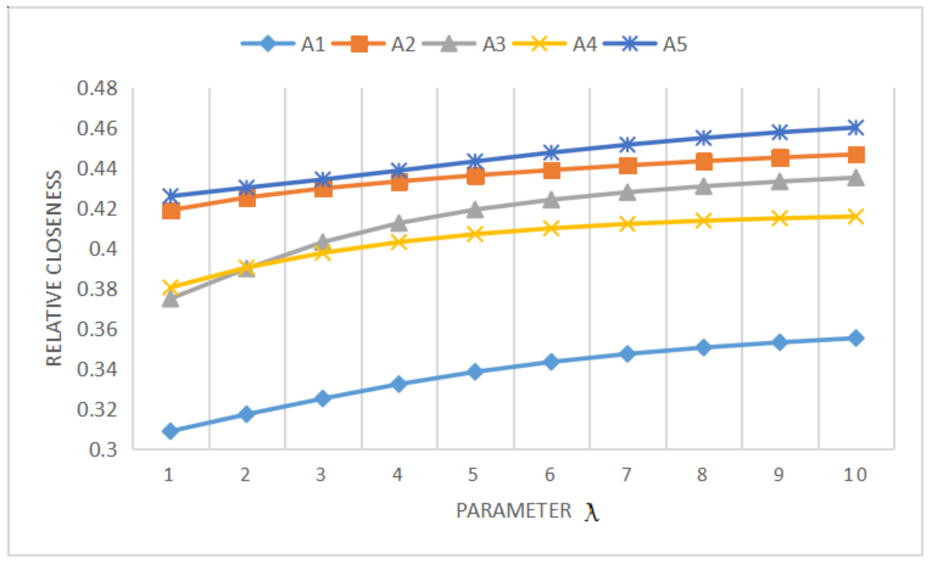
Based on entropy measure $E_1$, we can use the improved method in Section 4 to get the ranking order of these five alternatives. To reflect the influence of the parameter $\lambda$ in (7) on the ranking results, the value of $\lambda$ ranges from 1 to 10 with Step 1 and the ranking orders are summarized in

Table 7. Ranking results taking different values of the parameter $\lambda$.

$\mathit{\lambda }$	${\mathit{A}}_1$	${\mathit{A}}_2$	${\mathit{A}}_3$	${\mathit{A}}_4$	${\mathit{A}}_5$	Ranking
1	$0.3089$	$0.4190$	$0.3749$	$0.3805$	$0.4260$	$A_1\succ A_3\succ A_4\succ A_2\succ A_5$
2	$0.3174$	$0.4254$	$0.3900$	$0.3904$	$0.4302$	$A_1\succ A_3\succ A_4\succ A_2\succ A_5$
3	$0.3252$	$0.4299$	$0.4031$	$0.3977$	$0.4343$	$A_1\succ A_4\succ A_3\succ A_2\succ A_5$
4	$0.3324$	$0.4334$	$0.4126$	$0.4031$	$0.4387$	$A_1\succ A_4\succ A_3\succ A_2\succ A_5$
5	$0.3385$	$0.4364$	$0.4193$	$0.4071$	$0.4433$	$A_1\succ A_4\succ A_3\succ A_2\succ A_5$
6	$0.3434$	$0.4390$	$0.4242$	$0.4100$	$0.4477$	$A_1\succ A_4\succ A_3\succ A_2\succ A_5$
7	$0.3474$	$0.4414$	$0.4280$	$0.4122$	$0.4516$	$A_1\succ A_4\succ A_3\succ A_2\succ A_5$
8	$0.3506$	$0.4434$	$0.4309$	$0.4138$	$0.4550$	$A_1\succ A_4\succ A_3\succ A_2\succ A_5$
9	$0.3532$	$0.4452$	$0.4333$	$0.4150$	$0.4578$	$A_1\succ A_4\succ A_3\succ A_2\succ A_5$
10	$0.3553$	$0.4468$	$0.4352$	$0.4159$	$0.4602$	$A_1\succ A_4\succ A_3\succ A_2\succ A_5$

. It shows that different values of $\lambda$ may produce different solutions to the invest problem. To sum up, two slightly different solutions are created, which are $A_1\succ A_3\succ A_4\succ A_2\succ A_5$ and $A_1\succ A_4\succ A_3\succ A_2\succ A_5$. Meanwhile, $A_1$ is always the best choice no matter what $\lambda$ is. Figure 1 plots the movement of $R{C}_i(i=1,\cdots ,5)$ with a variation in $\lambda$. Along with the increase of $\lambda$, relative closeness $R{C}_i(i=1,\cdots ,5)$ of the five nations steadily increase. Through further observation, the curve of $R{C}_3$ crosses the curve of $R{C}_4$, when $\lambda$ is changed from 1 to 3.

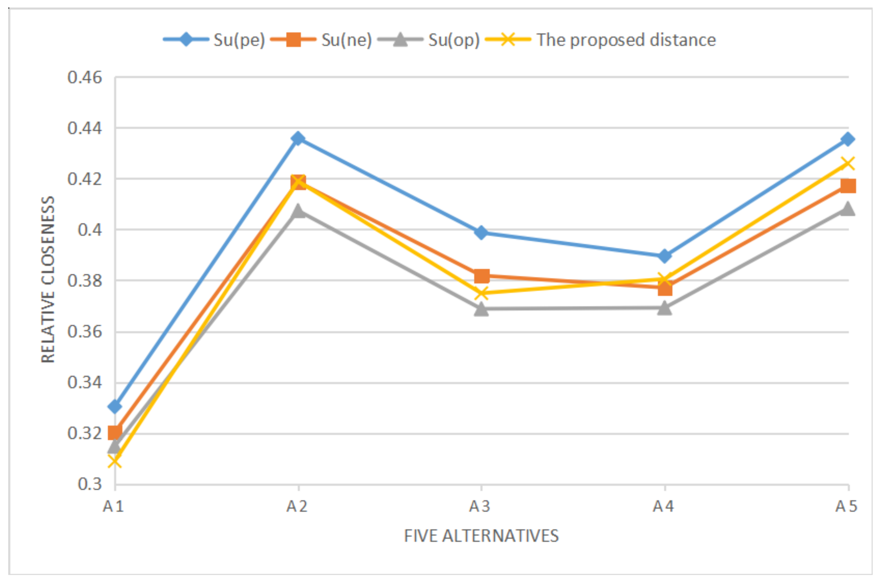
Su and his coworkers defined a series of distance measures of DHFSs in 2015 [18]. Among these measures, the elements of membership or non-membership degrees in two DHFEs should be adjusted as introduced in Section 1. For the convenience of comparison, suppose that $\lambda =1$ and $w={(0.2565,0.1669,0.1305,0.0985,0.1172,0.0724,0.1580)}^T$. It is noted that the attitude of the DM is assumed as optimism, pessimism or neutrality, in the process of solving evaluation problem through distance measure in [18]. With this assumption, the original DHFEs can be changed into the same length. For the sake of simplicity, Su’s distance measure with different attitudes i.e., optimism $(\delta =1)$, pessimism $(\delta =0)$ or neutrality $(\delta =0.5)$ are denoted as Su(op),Su(pe) and Su(ne), respectively. Using Su(op), Su(pe), Su(ne) and the proposed measure respectively, $R{C}_i$ and the ranking results of the five nations are obtained and shown in

Table 8. Ranking order of five nations derived from different distance measures.

Alternatives	${\mathit{RC}}_{\mathit{i}}\left(\mathit{proposed}\right)$	Ranking Order	${\mathit{RC}}_{\mathit{i}}\left(\mathit{Su}\left(\mathit{pe}\right)\right)$	Ranking Order	${\mathit{RC}}_{\mathit{i}}\left(\mathit{Su}\left(\mathit{ne}\right)\right)$	Ranking Order	${\mathit{RC}}_{\mathit{i}}\left(\mathit{Su}\left(\mathit{op}\right)\right)$	Ranking Order
$A_1$	$0.3089$	1	$0.3304$	1	$0.3203$	1	$0.3148$	1
$A_2$	$0.4190$	4	$0.4358$	5	$0.4187$	5	$0.4074$	4
$A_3$	$0.3749$	2	$0.3987$	3	$0.3819$	3	$0.3688$	2
$A_4$	$0.3805$	3	$0.3895$	2	$0.3771$	2	$0.3692$	3
$A_5$	$0.4260$	5	$0.4355$	4	$0.4173$	4	$0.4083$	5

. To facilitate the comparison analysis, $R{C}_i$ under four different measures are plotted in Figure 2.

As shown in Table 8, the ranking result obtained by the proposed distance measure is significantly different from that using distance in [18]. More specifically, even adopting the distance measure proposed by Su, the ordering of the alternatives has also changed due to different attitude of DMs. Using Su(op), Su(pe) and Su(ne), the ranking of $A_3$ go from the third to the second and the ranking of $A_5$ is demoted from the fourth to the fifth. The main reason for this difference is that the values are added in DHFEs based on different risk attitude of DMs in the process of calculation. If more elements are added, the ranking of alternatives will be unstable. However, the proposed distance measure need not adjust any DHFEs, so the obtained decision-making result is more objective and reasonable.

6. Conclusions

DHFS is one of the most powerful tools for expressing uncertain and fuzzy information. In the decision-making process, the distance between two different DHFEs should be measured. According to the existing methods, DMs always must add values into shorter DHFEs based on risk preference. Adding values into dual hesitant fuzzy elements not only makes the information lose their original feature and thus increases the subjectivity of decision-making to some extent.

In this study, motivated by the ideas of existing literature, we first develop some novel distance and similarity measures for DHFS without adjusting any DHFEs, including dual hesitant normalized Hamming distance, dual hesitant normalized Euclidean distance, generalized dual hesitant normalized distance, the weighted distance measures as well as the corresponding distance measures in the continuous situations. Then two types of entropy measures are given based on the complementary set of DHFS and the fuzziest set, respectively. The proposed entropy measures can be used to determine the weights of evaluation attributes. Making use of these novel information measures, an improved TOPSIS method with evaluation values in the form of DHFE is proposed to deal with MADM problems.

To illustrate the applicability and advantages of the proposed method, we consider two practical examples, which are the investment selection problem and the choice of countries to import from iron and steel in China, respectively. Compared to several existing methods, the results of experiments show that the proposed method seems to be more comprehensive, which can provide more flexible and reasonable choices to DMs. The more study on how to measure different DHFEs and solve other MADM problems in a dual hesitant fuzzy environment will be performed in the future.

References

- Zadeh, L.A. Fuzzy sets. Inf. Control. 1965, 8, 338–353. [Google Scholar] [CrossRef] [Green Version]
- Dubois, D.; Prade, H. Fuzzy Sets and Systems: Theory and Applications; Academic Press: New York, NY, USA, 1980. [Google Scholar]
- Atanassov, K.T. Intuitionistic fuzzy set. Fuzzy Sets Syst. 1986, 20, 87–96. [Google Scholar] [CrossRef]
- Chen, H.P.; Xu, G.Q. Group decision making with incomplete intuitionistic fuzzy preference relations based on additive consistency. Comput. Ind. Eng. 2019, 135, 560–567. [Google Scholar] [CrossRef]
- Herrera, F.; Herrera-Viedma, E.; Verdegay, J.L. A model of consensus in group decision making under linguistic assessments. Fuzzy Sets Syst. 1996, 78, 73–87. [Google Scholar] [CrossRef]
- Joshi, D.K.; Beg, I.; Kumar, S. Hesitant probabilistic fuzzy linguistic sets with applications in multi-criteria group decision making problems. Mathematics 2018, 6, 47. [Google Scholar] [CrossRef]
- Miyamoto, S. Remarks on basics of fuzzy sets and fuzzy multisets. Fuzzy Sets Syst. 2005, 156, 427–431. [Google Scholar] [CrossRef]
- Krishankumar, R.; Ravichandran, K.S.; Ahmed, M.I.; Kar, S.; Peng, X. Interval-valued probabilistic hesitant fuzzy set based muirhead mean for multi-attribute group decision-making. Mathematics 2019, 7, 342. [Google Scholar] [CrossRef]
- Torra, V.; Narukawa, Y. On hesitant fuzzy sets and decision. In Proceedings of the 2009 IEEE International Conference on Fuzzy Systems, Jeju Island, Korea, 20–24 August 2009; pp. 1378–1382. [Google Scholar]
- Torra, V. Hesitant fuzzy sets. Int. J. Intell. Syst. 2010, 25, 529–539. [Google Scholar] [CrossRef]
- Zhu, B.; Xu, Z.S.; Xia, M.M. Dual hesitant fuzzy sets. J. Appl. Math. 2012, 2012, 879629. [Google Scholar] [CrossRef]
- Chen, N.; Xu, Z.S.; Xia, M.M. Correlation coefficients of hesitant fuzzy sets and their applications to clustering analysis. Appl. Math. Model. 2013, 37, 2197–2211. [Google Scholar] [CrossRef]
- Ye, J. Correlation coefficient of dual hesitant fuzzy sets and its application to multiple attribute decision making. Appl. Math. Model. 2014, 38, 659–666. [Google Scholar] [CrossRef]
- Chen, Y.F.; Peng, X.D.; Guan, G.H.; Jiang, H.D. Approaches to multiple attribute decision making based on the correlation coefficient with dual hesitant fuzzy information. J. Intell. Fuzzy Syst. 2014, 26, 2547–2556. [Google Scholar]
- Farhadinia, B. Correlation for dual hesitant fuzzy sets and dual interval-valued hesitant fuzzy sets. Int. J. Intell. Syst. 2014, 29, 184–205. [Google Scholar] [CrossRef]
- Tyagi, S.K. Correlation coefficient of dual hesitant fuzzy sets and its applications. Appl. Math. Model. 2015, 39, 7082–7092. [Google Scholar] [CrossRef]
- Hu, J.H.; Zhang, Y.; Zhang, X.L.; Chen, X.H. Similarity and entropy measures for hesitant fuzzy sets. Int. Trans. Oper. Res. 2018, 25, 857–886. [Google Scholar] [CrossRef]
- Su, Z.; Xu, Z.S.; Liu, H.F.; Liu, S.S. Distance and similarity measures for dual hesitant fuzzy sets and their applications in pattern recognition. J. Intell. Fuzzy Syst. 2015, 29, 731–745. [Google Scholar] [CrossRef]
- Singh, P. Distance and similarity measures for multiple-attribute decision making with dual hesitant fuzzy sets. Comput. Appl. Math. 2017, 36, 111–126. [Google Scholar] [CrossRef]
- Xue, M.; Fu, C.; Chang, W.J. Determing the parameter of distance measure between dual hesitant fuzzy information in multiple attribute decision making. Int. J. Fuzzy Syst. 2018, 20, 2065–2082. [Google Scholar]
- Garg, H.; Kaur, G. Algorithm for probabilistic dual hesitant fuzzy multi-criteria decision-making based on aggregation operators with new distance measures. Mathematics 2018, 6, 280. [Google Scholar] [CrossRef]
- Liu, C.; Tang, G.L.; Liu, C.Q.; Liu, P.D. Multi-criteria decision making based on interval-valued dual hesitant uncertain linguistic generalized Banzhaf Choquet integral operator. Syst. Eng. Theory Pract. 2018, 38, 1213–1216. [Google Scholar]
- Su, Z.; Xu, Z.S.; Zhao, H.; Liu, S.S. Distribution-based approaches to deriving weights from dual hesitant fuzzy information. Symmetry 2019, 11, 85. [Google Scholar] [CrossRef]
- Zhao, N.; Xu, Z.S. Entropy measures for dual hesitant fuzzy information. In Proceedings of the 2015 Fifth International Conference on Communication Systems and Network Technologies, Gwalior, India, 4–6 April 2015; pp. 1152–1156. [Google Scholar]
- Ye, J. Cross-entropy of dual hesitant fuzzy sets for multiple attribute decision-making. Int. J. Decis. Support Syst. Technol. 2016, 8, 20–30. [Google Scholar] [CrossRef]
- Yan, F.F.; Wei, C.P.; Ge, S.N. Entropy measures for dual hesitant fuzzy sets and their application of multi-attribute decision making. Math. Pract. Theory 2018, 48, 131–139. [Google Scholar]
- Wang, H.J.; Zhao, X.F.; Wei, G.W. Dual hesitant fuzzy aggregation operators in multiple attribute decision making. J. Intell. Fuzzy Syst. 2014, 26, 2281–2290. [Google Scholar]
- Yu, D.J.; Zhang, W.Y.; Huang, G. Dual hesitant fuzzy aggregation operators. Technol. Econ. Dev. Econ. 2015, 22, 194–209. [Google Scholar] [CrossRef]
- Yu, D.J. Arpsimedean aggregation operators based on dual hesitant fuzzy set and their application to GDM. Int. J. Uncertain. Fuzziness Knowl. Based Syst. 2015, 23, 761–780. [Google Scholar] [CrossRef]
- Wang, L.; Shen, Q.G.; Zhu, L. Dual hesitant fuzzy power aggregation operators based on Arpsimedean t-conorm and t-norm and their application to multiple attribute group decision making. Appl. Soft Comput. 2016, 38, 23–50. [Google Scholar] [CrossRef]
- Tu, H.N.; Wang, C.Y.; Zhou, X.Q.; Tao, S.D. Dual hesitant fuzzy aggregation operators based on Bonferroni means and their applications to multiple attribute decision making. Ann. Fuzzy Math. Inform. 2017, 14, 265–278. [Google Scholar]
- Xu, Y.J.; Rui, D.; Wang, H.M. Dual hesitant fuzzy interaction operators and their application to group decision making. J. Ind. Prod. Eng. 2018, 32, 273–290. [Google Scholar] [CrossRef]
- Tang, X.A.; Yang, S.L.; Pedrycz, W. Multiple attribute decision-making approach based on dual hesitant fuzzy frank aggregation operators. Appl. Soft Comput. 2018, 68, 525–547. [Google Scholar] [CrossRef]
- Zhang, N.; Jian, J.; Su, J.F. Dual hesitant fuzzy linguistic power-average operators based on archimedean t-Conorms and t-Norms. IEEE Access 2019, 7, 40602–40624. [Google Scholar] [CrossRef]
- Wang, J.; Lu, J.P.; Wei, G.W.; Lin, R.; Wei, C. Models for MADM with single-valued neutrosophic 2-tuple linguistic muirhead mean operators. Mathematics 2019, 7, 442. [Google Scholar] [CrossRef]
- Zhu, B.; Xu, Z.S. Some results for dual hesitant fuzzy sets. J. Intell. Fuzzy Syst. 2014, 26, 1657–1668. [Google Scholar]
- Hu, J.H.; Zhang, X.L.; Chen, X.H.; Liu, Y.M. Hesitant fuzzy information measures and their application in multi-criteria decision making. Int. J. Syst. Sci. 2015, 47, 62–76. [Google Scholar] [CrossRef]
- Liao, H.C.; Xu, Z.S.; Zeng, X.J. Novel correlation coefficients between hesitant fuzzy sets and their application in decision making. Knowl. Based Syst. 2015, 82, 115–127. [Google Scholar] [CrossRef]
- Meng, F.Y.; Chen, X.H. Correlation coefficients of hesitant fuzzy sets and their application based on fuzzy measures. Cogn. Comput. 2015, 7, 445–463. [Google Scholar] [CrossRef]
- De Luca, A.; Termini, S. A definition of a non-probabilistic entropy in the setting of fuzzy sets theory. Inf. Control 1972, 20, 301–312. [Google Scholar] [CrossRef]
- Szmidt, E.; Kacprzyk, J. Entropy for intuitionistic fuzzy sets. Fuzzy Sets Syst. 2001, 118, 467–477. [Google Scholar] [CrossRef]
- Yagar, R.R. On the measure of fuzziness and negation Part I: Membership in the unit interval. Int. J. Gen. Syst. 1979, 5, 221–229. [Google Scholar] [CrossRef]
- Shang, X.G.; Jiang, W.S. A note on fuzzy information measures. Pattern Recognit. Lett. 1997, 18, 425–432. [Google Scholar] [CrossRef]
- Farhadinia, B. Information measures for hesitant fuzzy sets and interval-valued hesitant fuzzy sets. Inf. Sci. 2013, 204, 129–144. [Google Scholar] [CrossRef]
- Hwang, C.L.; Yoon, K. Multiple Attribute Decision Making: Methods and Applications; Springer: Berlin/Heidelberg, Germany; New York, NY, USA, 1981. [Google Scholar]
- Mardani, A.; Jusoh, A.; Zavadskas, E.K. Fuzzy multiple criteria decision-making techniques and applications-two decades review from 1994 to 2014. Expert Syst. Appl. 2014, 42, 4126–4148. [Google Scholar] [CrossRef]
- Yang, P.L.; Liu, X.; Xu, G.Q. A dynamic weighted TOPSIS method for identifying influential nodes in complex networks. Mod. Phys. Lett. B 2018, 32, 1850216. [Google Scholar] [CrossRef]
- Kumar, K.; Garg, H. Connection number of set pair analysis based TOPSIS method on intuitionistic fuzzy sets and their application to decision making. Appl. Intell. 2018, 48, 2112–2119. [Google Scholar] [CrossRef]
- Farhadinia, B.; Herrera-Viedma, E. Multiple criteria group decision making method based on extended hesitant fuzzy sets with unknown weight information. Appl. Soft Comput. 2019, 78, 310–323. [Google Scholar] [CrossRef]
Figure 1.
Relative closeness of the five nations with a variation in .
Figure 2.
Relative closeness derived from different distance measures.