Closing Gaps in Geometrically Frustrated Symmetric Clusters: Local Equivalence between Discrete Curvature and Twist Transformations

1
Quantum Gravity Research, Topanga, CA 90290, USA
2
Faculty of Health, Engineering and Sciences, University of Southern Queensland, Toowoomba, QLD 4350, Australia
*
Author to whom correspondence should be addressed.
Mathematics 2018, 6(6), 89; https://doi.org/10.3390/math6060089
Submission received: 24 April 2018
/
Revised: 22 May 2018
/
Accepted: 23 May 2018
/
Published: 25 May 2018
Abstract
:In geometrically frustrated clusters of polyhedra, gaps between faces can be closed without distorting the polyhedra by the long established method of discrete curvature, which consists of curving the space into a fourth dimension, resulting in a dihedral angle at the joint between polyhedra in 4D. An alternative method—the twist method—has been recently suggested for a particular case, whereby the gaps are closed by twisting the cluster in 3D, resulting in an angular offset of the faces at the joint between adjacent polyhedral. In this paper, we show the general applicability of the twist method, for local clusters, and present the surprising result that both the required angle of the twist transformation and the consequent angle at the joint are the same, respectively, as the angle of bending to 4D in the discrete curvature and its resulting dihedral angle. The twist is therefore not only isomorphic, but isogonic (in terms of the rotation angles) to discrete curvature. Our results apply to local clusters, but in the discussion we offer some justification for the conjecture that the isomorphism between twist and discrete curvature can be extended globally. Furthermore, we present examples for tetrahedral clusters with three-, four-, and fivefold symmetry.
Keywords:
quasicrystals; geometric frustration; space packing; tetrahedral packing; discrete curvature; twist transformationPASC:
61.44.BrMSC:
52C17; 52C23; 05B40
1. Introduction
Geometric frustration is the failure of local order to propagate freely throughout space, where local order refers to a local arrangement of geometric shapes, and free propagation refers to the filling of the space with copies of this arrangement without gaps, overlaps, or distortion [1]. Classical examples include 2D pentagonal order and 3D icosahedral order, where the dihedral angle of the unit cell does not divide , and therefore it is not compatible with the translations [1]. A traditional solution to relieve the frustration in nD is to curve the space into D so that the vertices of the prototiles (pentagons in the 2D example) all land on an n-sphere (dodecahedron) and the discrete curvature is concentrated at the joints between prototiles (dodecahedral edges and vertices). This eliminates the deficit in the dihedral angle to close a circle. As in the above example, pentagonal order can propagate freely on a two-sphere, for example a dodecahedron or icosahedron, while icosahedral order can propagate freely on a three-sphere, for example, a 600-cell or 120-cell. This hypersphere solution, described more fully in Section 2, gives only a finite propagation of the local order, since the spherical space is finite, but sections of intersecting hyperspheres can be used as building blocks to achieve infinite propagation, resulting in quasicrystalline order (for a comprehensive study of geometric frustration and its treatment with discrete curvature, see Reference [1]).
A case of particular interest is that of tetrahedral packings in 3D. For regular tetrahedra, the dihedral angle of does not divide , thus leaving gaps between them when arranged in edge-sharing (Figure 1a) or vertex-sharing (Figure 1b) configurations. The presence of these gaps, i.e., the geometric frustration, means they cannot tile 3D space. However, the tetrahedron configuration is the densest local sphere packing in 3D, and often gives the lowest energy state for four atoms. The packing of regular tetrahedra is therefore a non-trivial problem that is of interest to chemists and physicists, as well as mathematicians [2].
Given some edge- or vertex-sharing cluster of polyhedra such as that shown in Figure 1, one way to close the gaps isometrically (i.e., without distorting the polyhedra) is to discretely curve the space, as mentioned above. It turns out, however, that this is not the only way. For a particular vertex-sharing configuration, Fang et al. [3] showed an alternative called the twist method, an isometry on the tetrahedra that closes the gaps without recourse to a fourth dimension. In their approach, which we review in Section 2 and Section 3, each tetrahedron is rotated in 3D around an individual axis; with the correct choice of axes and rotation angles, adjacent face planes of neighbouring tetrahedra are made to coincide, although the faces themselves do not exactly coincide within those planes. In a second paper from Fang et al. [4], the twist method was used, among other methods, to construct a novel quasicrystal.
In this paper, we show that the twist method works quite generally to close gaps between face planes for polyhedron clusters with any dihedral angle and gap size. We derive a general formula for the required twisting angle, as well as for the bending angle required in the discrete curvature method, with the surprising result that the angles are the same. Furthermore, the twist’s misalignment of faces within a shared plane is actually an analogue of the discrete curvature’s dihedral angle between polyhedra, and we derive expressions for these angles, showing that they also match. Due to the complicated nature of the rotations, especially involving higher dimensions, we include illustrations and detailed explanations in the hope that this will make our constructions more clear.
The paper is organized as follows. Section 2 provides a more detailed description of the discrete curvature and the twist methods, and Section 3 explains the connection between them. In Section 4, we construct the transformations for the two methods and derive their matching formulae for the transformation and joint angles, respectively. In Section 5, we briefly discuss the possibility of global extension. An appendix is included where we use the results of Section 4 to compute the transformation and joint angles for a few examples of tetrahedra in edge-sharing and vertex-sharing configurations. Similar calculations can be applied to any symmetric cluster of polyhedra.
2. Description of Discrete Curvature and Twist Methods
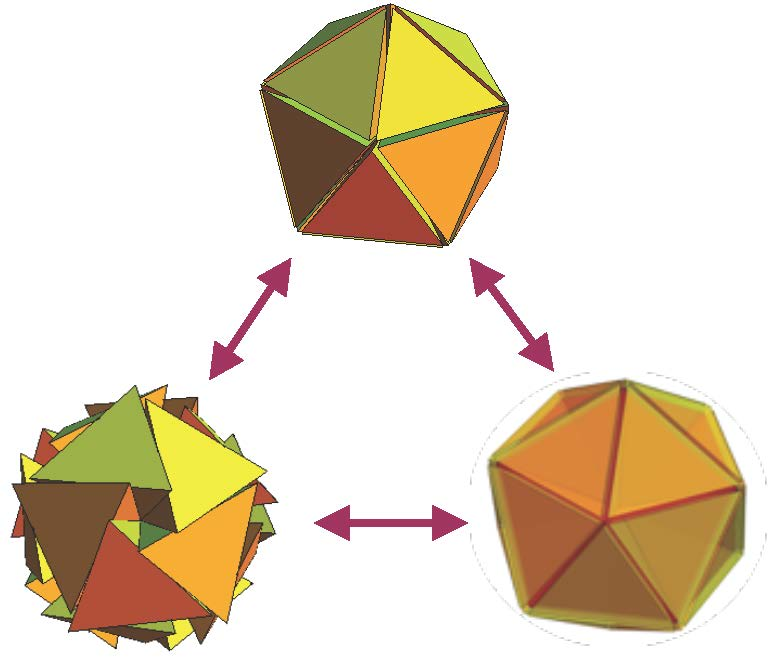
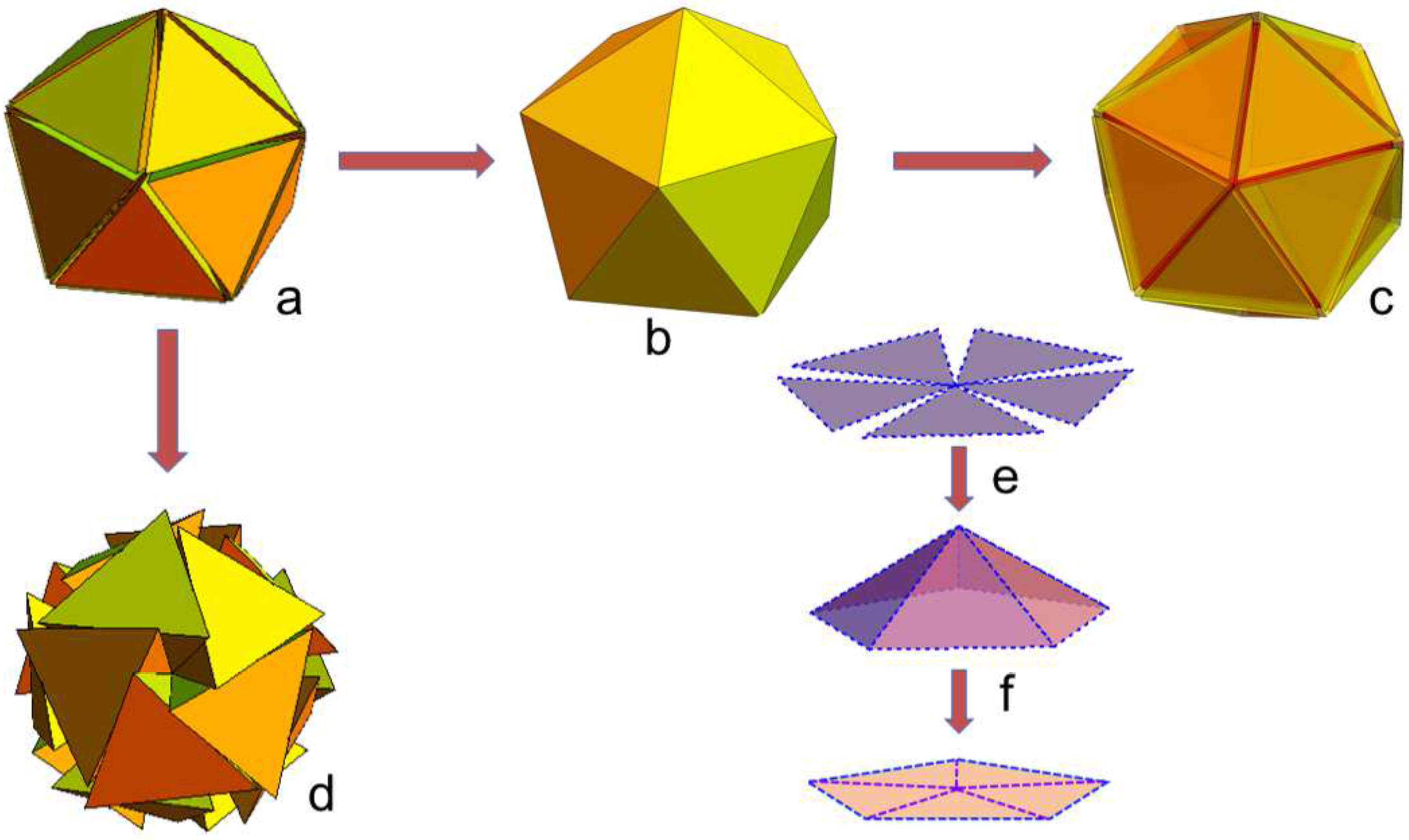
A cluster of congruent polyhedra with a shared vertex or edge can be symmetrically arranged so that the gaps between them are evenly distributed. Figure 2a shows such an arrangement of 20 regular tetrahedra sharing a vertex. The other images in Figure 2 illustrate how the gaps can be closed, while maintaining congruence of the tetrahedra, by discrete curvature (Figure 2b), distortion (Figure 2c), or twist (Figure 2d). We mention distortion because it is the result of the 3D projection of discrete curvature, and it can be important in atomic configurations, but, in this paper, we restrict our attention to the relation between the isometric methods, which close the gaps by some type of rotation.
In these isometric methods, the angle by which the polyhedra are rotated from the symmetric, gapped configuration is called the transformation angle. When the gaps are closed, each pair of neighbouring polyhedra meets in a plane, but deviates by some joint angle from being simple reflections of each other across that plane. For each case these angles are described in more detail below.
2.1. Discrete Curvature
Discretely curving the space permits unhindered propagation of the local pattern with all vertices free of imperfect local symmetries. However, this method requires an extra dimension. For example, the 20-tetrahedron cluster in Figure 2a can be bent into the 4th dimension to close all the gaps between tetrahedra, while keeping their shared vertex invariant (an analogue from 2D to 3D is shown in Figure 2e). As the gaps close, the tetrahedra form a sort of pyramidal cap around this vertex. The outer faces of the tetrahedra constitute the rim of this cap and form an icosahedron; they are shown in Figure 2b, which is a slice through the 3D space containing the rim. The vertex of the cap is not at the 3D centre of Figure 2b, but is displaced out in the 4th dimension. Compare this to Figure 2f, where the outer edges of the triangles form a pentagon in a 2D plane while the shared vertex point is displaced out of that plane.
The transformation angle here is the angle by which each tetrahedron rotates into the fourth dimension, and it can be positive or negative, corresponding to bending up or down in 4D. When the faces meet, the joint angle is the dihedral angle between adjacent tetrahedra. At that point, the original geometric frustration of the gapped configuration has vanished, but an encoding of it remains in the form of this joint angle.
With the 20 tetrahedra arranged to form the pyramidal cap, all their vertices (including the central, shared vertex) belong to a 3-sphere that lives in 4D. Their local icosahedral pattern can propagate freely on the 3-sphere until it forms a 4D polytope, the 600-cell, each of whose 120 vertices is surrounded by a 20-tetrahedron cluster in the configuration of Figure 2b. Because the 600-cell is a discretized version of the 3-sphere, with the curvature concentrated in discrete amounts at edges and vertices, we refer to this as having discrete curvature. That is not to say that the space of an individual tetrahedron is curved: rather, it is the space of the whole cluster that is curved, with that curvature being concentrated at the joints between tetrahedra.
2.2. Twist
As an alternative to bending the cluster into the fourth dimension, one may close the gaps between face planes by twisting the cluster in 3D. Each tetrahedron in Figure 2a can be rotated around an axis which connects its centroid with the shared vertex, leading to configuration Figure 2d, as was previously shown by Fang et al. [5]. Other examples are given in the following section, with illustrations in Table 1 (an interactive dynamic illustration is available online, please check the Supplementary Materials). We use the name “twist method” because tetrahedra on opposite sides of the cluster are rotated in opposite senses relative to each other, giving the cluster a twisted structure. The transformation angle is again the angle by which each tetrahedron is rotated, and it can be positive or negative, resulting in either a left- or right-handed twisted cluster.
One can see in Figure 2d that the gap between adjacent faces is closed, while the gap between a group of neighbouring edges is enlarged into an empty pentagonal cone. This empty cone results from the fact that the two triangular faces in a given shared plane are misaligned. The angular difference between them is the joint angle, which, as in the case of discrete curvature, encodes the geometric frustration. In the pentagonal cone, the joint angle is manifest as the apex angle of a triangular face.
3. Equivalence between the Discrete Curvature and Twist Methods
The discrete curvature and twist methods are characterized by their transformation angles for closing the gaps and their joint angles encoding the geometric frustration. We initially noticed that, for the 20-tetrahedron cluster, both these angles are the same in the one case as in the other (in fact, both transformation angles equal the angle of R. Buckminster Fuller’s jitterbug rotation [6], although at present it is not clear why this should be so). This motivated further study of similar cases, wherein regular tetrahedra are arranged about a single shared edge or vertex in clusters of two-, three-, four- or fivefold symmetry. In each case the gaps between tetrahedral faces can be closed either by bending up to 4D or by twisting in 3D. The twisting is illustrated in the first four rows of Table 1, with dynamic versions online in the Supplementary Materials. (We ignore the twofold cluster because it is degenerate, although technically the results still apply).
To each twisted edge-sharing cluster, there corresponds a twisted vertex-sharing cluster that preserves the relative orientations of the tetrahedra and the axial symmetry. Table 1 shows that the twisted 20-tetrahedron cluster, denoted as 20 G, is a composition of twisted vertex-sharing fivefold clusters, and the vertex-sharing threefold cluster is a subset of this 20 G. Furthermore, the twisted vertex-sharing fourfold cluster has eight tetrahedra, with four in one orientation corresponding to a subset of the left-handed 20 G and the other four in the other orientation corresponding to a subset of the right-handed 20 G.
If one begins with the symmetrically gapped configuration, one can transform, by rotations in appropriate planes, to either the 20 G (3D twisted configuration) or the vertex cap of a 600-cell (4D curved configuration). In both cases, the number of tetrahedra sharing a common edge (or edge centre) is five, and the number sharing a common vertex is twenty. Moreover, the transformation angles in each case are the same, as are the resulting joint angles. We therefore refer to the 600-cell vertex cap as a 4D analogue of the 20 G. Similarly, the 16-cell vertex cap is the 4D analogue of the fourfold case, and the 5-cell vertex cap is the 4D analogue of the threefold case. In the twisting angle row of Table 1, E denotes the twisting angle of the tetrahedron around an axis connecting the midpoints of its central and peripheral edges to close the edge sharing cluster, V denotes the transformation angle to close the vertex-sharing cluster, and F denotes the joint angle where faces meet. For the angles in the 4D analogues, B denotes the transformation angle (the bending angle to close the gaps) and D the joint (dihedral) angle. In all three cases, both the transformation angle and the joint angle match, i.e., and . This finding implies that, at least locally, there is a perfect equivalence between encoding geometric frustration using the discrete curvature method and the twisting method.
4. Angle Matching between Discrete Curvature and Twist Transformations
In this section, we explicitly construct the transformations for the discrete curvature and twist methods, and show the equivalence of the respective angles. We use the Clifford algebra formalism because it is a clean and efficient algebraic encoding of geometric concepts. (Expressions for the transformation and joint angles can also be found by visualizing the structures and applying trigonometry, but Clifford algebra provides a more systematic way to articulate the construction. For the interested reader unfamiliar with Clifford algebra, useful introductions were provided in [7,8,9], and monograph references are in [10,11,12]). The transformations are constructed in parallel to exhibit not only the isogonism between the two methods, but also the parallel aspects in the geometric structure which are the cause of that isogonism.
We begin by defining intersecting bivectors F and , representing the face planes of two neighbouring polyhedra, as well as a number of auxiliary geometric elements. We then construct the two rotations—the twist in 3D and the discrete curve in 4D—showing that for some angle each transforms F and into the same bivector. From this, we compute the transformation and joint angles, and show their respective equivalence.
4.1. The Geometric Elements
4.1.1. Basic Definitions
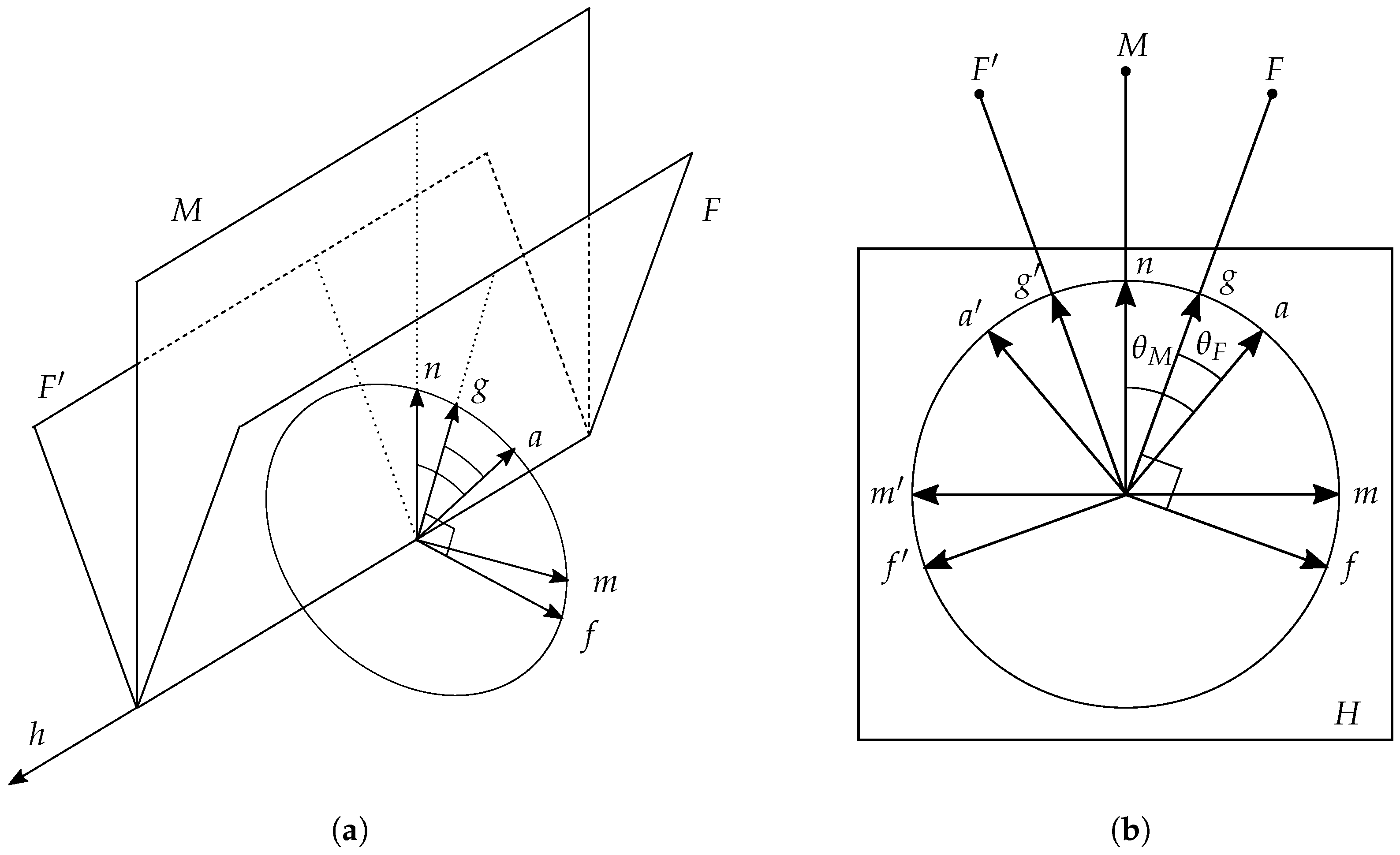
Let be the geometric algebra of with unit right-handed pseudoscalar I, and let be a unit vector orthogonal to I (and thus not in ). Thus I and span an with geometric algebra and unit pseudoscalar . In we denote the geometric (or Clifford) product by juxtaposition, with the inner and outer products indicated respectively by · and ∧. We define the following elements, which are illustrated in Figure 3.
In , let F and be distinct unit bivectors with a common unit vector h (all bivectors defined here and after are actually 2-blades, or “simple” bivectors, being factorizable as the product of two vectors).
Let unit vectors g and be defined by and . Since the bivectors are distinct, . Assume F and are oriented such that (if gives a left-handed trivector, swap the labels of F and to make it right handed).
Let unit vectors f and be defined by , . Thus, f and are the respective normals to F and within the 3-space of I, but with opposite handedness.
Let be a unit bivector.
We define the unit vector , used to generate reflections which are important for the discrete curvature transformation. Its normal in the H plane is , while its normal in I is the mirror plane . We call M the “mirror” because is the reflection of F in it (Section 4.1.2, Equation (2)). The mirror in J (i.e., in ) is , the hyperplane normal to m.
Now within H, we choose any unit vector a lying between g and m, and define the angles and between a and the bivectors F and M, respectively. Equivalently, these are the respective angles a makes with g and n. We define also as the counterpart to a, reflected by m.
4.1.2. Reflections
For an arbitrary even or odd grade multivector A, a reflection in the subspace normal to m (briefly, a reflection by m) is given by , where the sign is positive or negative according as A is even or odd. Therefore, the reflection of g by m is
Using the fact that , the reflections of F and f by m are
Indeed, quite generally, all vectors in the H plane are defined in pairs, the primed and unprimed versions being related by reflection by m. Of course, , while n is invariant under this reflection.
Within the H plane, reflection by m is equivalent to reflection in n, since n is the “hyperplane” in H normal to m. Outside that plane, however, the two are different. Reflections in n, important for the twist transformation, are written
where we have used the fact that H anticommutes with vectors lying in it, as well as with bivectors perpendicular to it, and that . One sees that the sign for reflection in a vector is opposite the sign for reflection by a vector (i.e., in its normal hyperplane).
Let us summarize the elements we have defined and their relationships, referring to Figure 3 for their illustration. We have vectors f, g, h, m, n, a, and and bivectors F, M, and H, as well as their primed counterparts reflected by m. With the exception of these can be seen in the figure, which shows the 3D subspace of I. They satisfy
In the definition of n, the sign was chosen so that g lies between m and n, and by inspecting the figure one readily sees the consequence that and are not obtuse for any choice of a between g and m. Vectors a and will now be used to define the rotation planes of the transformations.
4.2. Definitions of Transformations
Definition 1.
The discrete curvature transformation (briefly, the discrete curve) is a pair of rotations within, rotating unprimed and primed multivectors out of, in theandplanes respectively, by the transformation angle α. The rotations are implemented by the rotor C and its reflection,
where the tilde represents reversion,.
The transformation angleis the angle for which.
Definition 2.
The twist transformation (briefly, the twist) is a pair of rotations within, rotating unprimed and primed multivectors around the axes a and, respectively, by the transformation angle α. The rotations are implemented by the rotors T and,
The transformation angleis the angle for which.
Remark 1.
is the reflection of C by m, butis the reflection of T in n. A critical feature of the twist is that both T andhave the same angle, including sign, so their rotations have the same handedness; they are therefore related by reflection in a vector, not in a plane. Algebraically, the difference between the C and T rotors is manifest in the fact that m and n anticommute with(in the C exponent) but commute with I (in the T exponent).
4.3. Equivalence of Transformation Angles
It is well known (e.g., [1]) that, for any a between g and m, and for some angle , the discrete curve brings F and into coincidence. This is how, for example, gaps between edge-sharing polyhedra in can be closed to form a polytope in . Moreover, Fang et al. [3] have shown in a specific case that, for a certain vector a and some angle , the twist transformation also brings F and together. Our first result is that not only does the twist work for any vector a between g and m, but the angle for the twist is the same as for the discrete curve. We demonstrate this by using the transformations defined above to derive the same formula for the two transformation angles.
Theorem 1.
For arbitrary a in the H plane between vectors g and m, the twist and discrete curvature transformations both bring F andinto coincidence by rotation through the same angle, that is,.
Proof.
Under the transformations, reflections by m and in n lose the equivalence seen in Equation (6e). As F and are rotated by the discrete curve, they remain reflections of each other by m; as they are rotated by the twist, they remain reflections of each other in n, i.e.,
Therefore, rotating F and into coincidence implies and , or
where represents the k-grade part of the expression. These can be expanded by splitting F into parts that, respectively, commute and anticommute with a:
For C, we have used the fact that all bivectors in 3D commute with , so since commutes with a it also commutes with ; in like manner anticommutes with . For T, a similar argument applies to and . Next, to solve Equation (10) explicitly for the angles, we expand and as
The term in Equation (13) vanished because , so , and likewise for the term in Equation (14). The h is factored out of Equation (14) (next to last step) with the following justification: it anticommutes with both F and a, so it anticommutes with ; since it also anticommutes with m, it therefore commutes with ; hence, , allowing the mentioned factoring.
We see in Equations (13) and (14) that and satisfy the same equation. Without loss of generality, we can choose the angles to lie between and , and we conclude . Solving for the angle we find
where the denominator was simplified using the fact that is orthogonal to both a and m. Looking at Figure 3 we can write this in terms of the angles,
Since we defined a to lie between g and m, , both acute, so exists. ☐
Remark 2.
andhave the same sign, so. This result permits two solutions for α, differing by a sign. For the discrete curve, these correspond to curving “up” towardor “down” toward; for the twist, they correspond to right- or left-handed rotation about axis a. Since for each sign the twist has a solution matching the discrete curvature solution, we are justified in saying their angles are the same.
Remark 3.
We note incidentally that if the transformation vector a were not in the H plane, Equation (14) could still be satisfied for a twist, theterm leading to a quadratic in. However, no discrete curve could then satisfy Equation (13), since theterm, if it does not vanish, is linearly independent of the others.
The geometry of these constructions can be seen in Figure 4, Figure 5 and Figure 6. We first consider the discrete curve, shown in Figure 4. Since h is left invariant, we ignore it for now and picture the 3-space of . The triangle containing a is rotated in the plane, while that containing is rotated in the plane. Vectors g and are rotated along arcs until they meet at in the plane. At that point , and projects down to , closing the circular arc. At the same time, the unchanged is also perpendicular to m, so . This is what is expressed algebraically in Equation (10a), which permits the solution for .
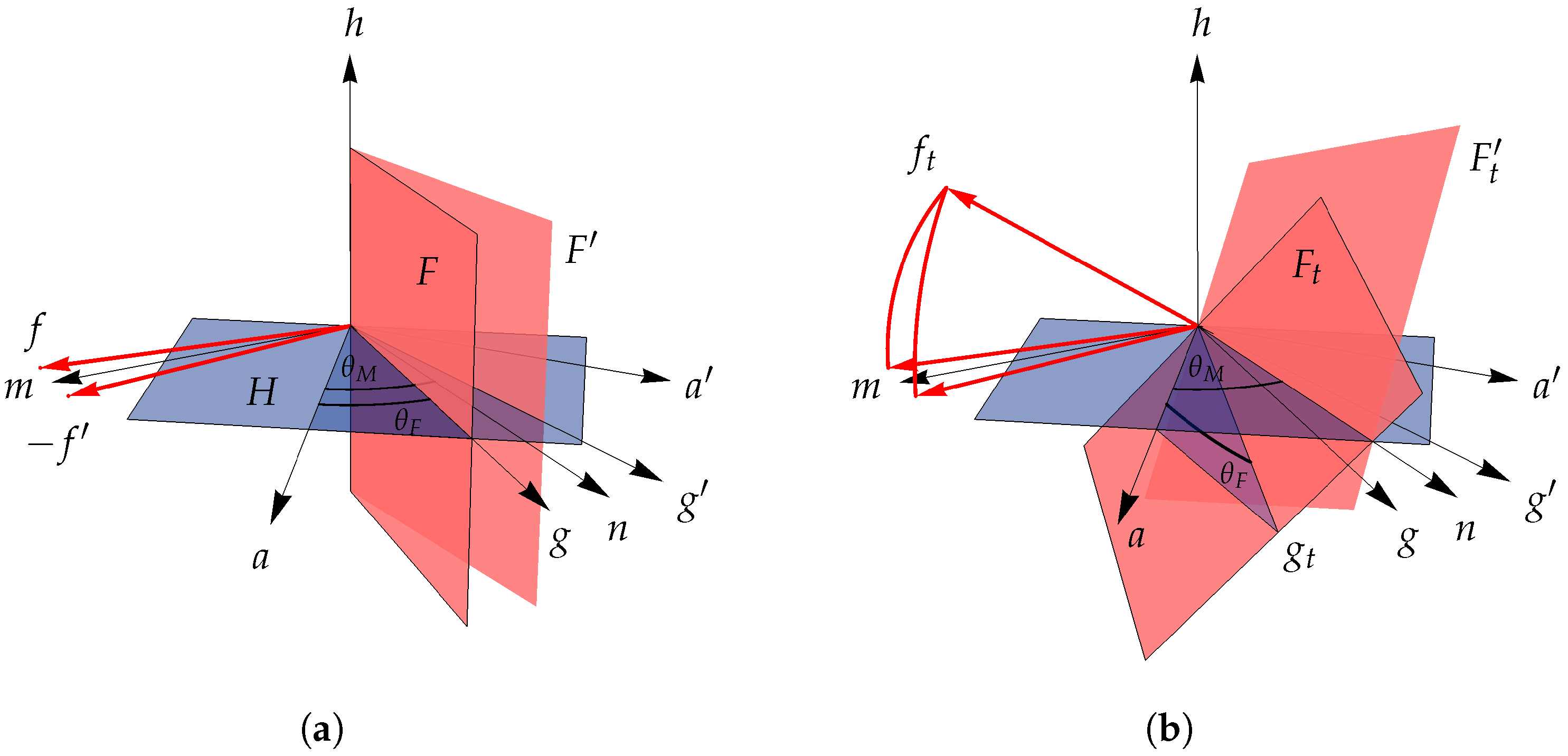
We next consider the twist, as shown in Figure 5. F and are rotated around a and , respectively, until they meet in , which contains n. This is expressed algebraically by Equation (10b), which permits the solution for . The similarity of this to the discrete curve is most easily seen by looking at the normal vectors f and , which follow arcs under the T transformation congruent to those followed by g and under the C transformation (Figure 4). This illustrates why the transformation angle is the same in both cases.
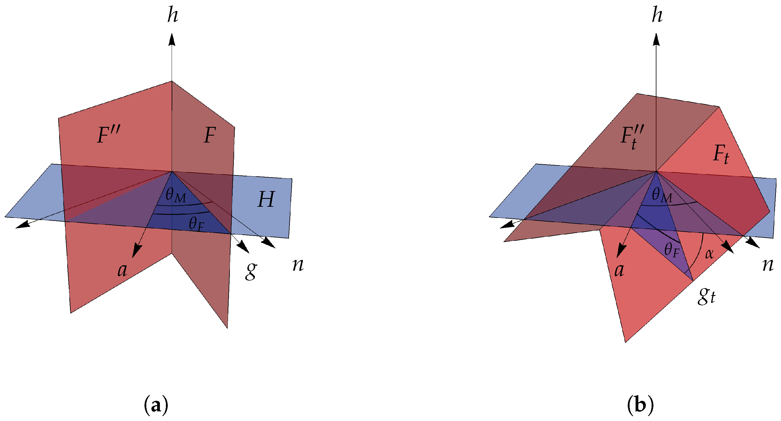
Figure 6 is a second illustration of the twist, where we leave out and show instead a new bivector , which is the reflection of F in the plane. Whereas F and represent adjacent face planes of neighbouring polyhedra brought together by being twisted around different axes, F and represent two face planes of a single polyhedron, rotated together around a single axis. This figure shows most clearly how the polyhedron’s actual dihedral angle is effectively enlarged in the H plane to match the target dihedral angle .
4.4. Equivalence of Joint Angles
Having established the equivalence of the transformation angles, we now turn to the joint angles. The two face planes F and live initially in the same , with unit trivector . The sign on the primed vectors is due to them being mirror reflections of the unprimed ones across M (one can see in Figure 3 that has the opposite handedness of ). The discrete curve and the twist are each constructed so as to bring the bivectors and into coincidence, but they do not in general align each individual vector with its primed counterpart. This misalignment is what results in the joint angles between polyhedra where the face planes meet.
Under the discrete curvature transformation, the two rotations C and have different actions on the original 3D space, so that is not the same as . More specifically, the vectors within F and do converge (g and are brought together in the final state, and is left invariant), but the normal vector does not become , because along the plane the 3-spaces of and meet at a bent joint.
Definition 3.
For the discrete curvature transformation, when, the joint angleis the angle inbetween trivectorsand. This is equivalent to the angle betweenand.
Remark 4.
If F andare faces of two distinct polyhedra brought together by the discrete curve to form two cells of anpolytope, then the joint angle thus defined is their exterior dihedral angle, supplementary to the ordinary interior dihedral angle.
Under the twist, the situation is reversed. T and leave I and invariant, so implies that . In this case, it is and that are twisted relative to and within the final plane, and their relative angle is the joint angle for the twist transformation.
Definition 4.
For the twist transformation, the joint angleis the angle in theplane betweenand.
Remark 5.
In an edge-sharing cluster of n polyhedra, the twist splits the shared edge into n distinct edges, leaving a void in the shape of an n-sided pyramidal cone (see row 2 of Table 1). For a vertex-sharing cluster, the nearest neighbour edges emanating from the shared vertex form a similar pyramidal cone. The joint angle is the angle between adjacent edges, i.e., the apex angle of the triangular sides of that pyramid.
In either case (discrete curvature or twist), the joint angle can be thought of as the angular relationship between the orthonormal triads f, g, h and , , h after they have been transformed. We now come to our second result, which is that both transformations yield the same joint angles.
Theorem 2.
The joint angles in the cases of discrete curvature and twist are the same, i.e.,.
Proof.
The proof is by direct computation of the half angles and (a briefer derivation than for the full angles).
Vector m bisects the angle between and , while n bisects the angle between and , for
Therefore,
For the twist T, it is straightforward to calculate using our explicit expression for T, but a more direct route to the result is found by using the fact that , which can be seen by looking at Figure 5. This is justified more rigorously by noting that n lies in (see Equation (10b)), so , while also . Hence, is perpendicular to any bivector containing . In particular, it is perpendicular to . However, also contains the invariant axis , and so is proportional to . Therefore, , or
using and . This can then be solved for
For , the computation is analogous. With , and also (Equation (10a), with lying in ), we find is perpendicular to any bivector containing . In particular, it is perpendicular to , which contains the invariant vector ( is orthogonal to both a and , which together form the plane of the rotation; it is the vector in H that remains invariant while H is rotated to ). Thus, , or
using and . Since , this can be solved for
The preceding proofs apply to any two bivectors F and that share a line of intersection. If these are the planes of adjacent faces of two edge-sharing or vertex-sharing polyhedra, we apply the respective rotations to each polyhedron as a whole. For a cluster of congruent polyhedra symmetrically arranged about a shared edge or vertex, each pair of adjacent face planes can be merged by simultaneously rotating all the polyhedra in the cluster, as illustrated for tetrahedral clusters in Table 1. In Appendix A, we apply the formula to several such clusters and show the explicit calculation of their transformation and joint angles.
5. Discussion and Outlook
In an attempt to fill flat 3D space, clusters of congruent polyhedral are geometrically frustrated—all arrangements with shared edges or vertices leave gaps between some of their neighbouring faces. A well-known isometric method for relieving this frustration and bringing those faces together uses discrete curvature, bending the cluster into the fourth dimension [1]. An alternative isometry is the twisting method, which involves the twisting of the cluster in 3D and thus does not require a fourth dimension.
In this paper, we have shown not only that twisting works quite generally, but also that the twisted structure entails the same transformation angle (relative to the symmetric, gapped configuration) and the same joint angle as the discretely curved one. We give the general formulae for the transformation and joint angles based on the dihedral angle of the polyhedra and the angle between adjacent polyhedra, thus simplifying the calculations required when applying our method.
The application of the twisting method to clusters of regular tetrahedra is particularly appealing, both because the tetrahedron is the simplest platonic solid, and because of its role in sphere packing, a case of interest for several research fields [2]. Therefore, we have presented the computations of the actual angles for tetrahedra in edge-sharing and vertex-sharing clusters with 3-, 4-, and 5-fold symmetry.
In this study, we have considered the particular case of clusters that share a single edge or vertex, but one would naturally like to know if our results could be generalized to larger groupings. We do know that, with the discrete curvature method, the local order can propagate beyond the local cluster, and that infinite propagation can be achieved with quasicrystalline order [1]. We also know that, for the 20 G, a twisted cluster whose 4D analogue is the vertex cap of a 600-cell, the local order can likewise be propagated indefinitely to form a quasicrystal, and that the same quasicrystal can be created by decorating a 3D slice of the Elser-Sloane quasicrystal, which is itself a network of intermeshing 600-cells [4,13]. In addition, the current paper has shown that, at least locally, the closing of gaps by the twist method, as well as the isogonism between the twist and the discrete curvature methods, are not coincidences due a particular configuration, but are quite general. This suggests that the success of the twist method at achieving global propagation from the 20 G is no coincidence either, and that a general method may be found to construct quasicrystals based on twisted structures to match those based on discretely curved structures. Perhaps to any corrugated 3-space complex of regular tetrahedra that does not deviate too far from a flat Euclidean 3-space, there corresponds some twisted structure in the flat space whose twist angles match the curvature angles of the corrugated structure. This is an interesting avenue for further research. If true, it would mean any such curved space complex could be represented by a twisted network of simplices in flat space.
Supplementary Materials
The following is available online at https://www.mdpi.com/2227-7390/6/6/89/s1. Figure S1: Twisting clusters. A set of dynamic, interactive images of edge- and vertex-sharing tetrahedral clusters that can be twisted, showing how the face planes are brought into coincidence.
Author Contributions
Conceptualization, K.I.; Formal analysis, R.C.; Investigation, F.F.; Visualization, F.F.; Writing—original draft, F.F. and R.C.
Acknowledgments
We thank Sinziana Paduroiu for her comments and for her generous help on technical writing and editing. We are grateful to Remy Mosseri for his suggestions and comments.
Conflicts of Interest
The authors declare no conflict of interest.
Appendix A. Computation of Angles for a Few Specific Cases
We apply the results of Section 4.3 and Section 4.4 to compute the transformation and joint angles for certain edge-sharing and vertex-sharing tetrahedron clusters with 3-, 4-, and 5-fold symmetry. Regular tetrahedra provide a simple and easy-to-visualize example of polyhedra that fail to tile 3D space. They may also be useful, if present results can be extended globally, in creating a twisted version of simplicial complexes to represent a discretely curved 3D manifold. For these reasons, it seems worthwhile to work out some tetrahedral examples in detail. Nevertheless, the principles apply equally to any symmetrically arranged polyhedral clusters, provided that they are congruent at their shared edge or vertex.
Appendix A.1. Shared Edge Configurations
We begin with a group of n congruent tetrahedra oriented symmetrically around a common edge (Figure A1 shows the case with regular tetrahedra). We define to be the unit vector directed from the centre of the shared edge out through the centroid of the ith tetrahedron (and hence toward the centre of that tetrahedron’s opposite, outer edge). These will all lie in a plane orthogonal to the shared edge, with angle between adjacent .
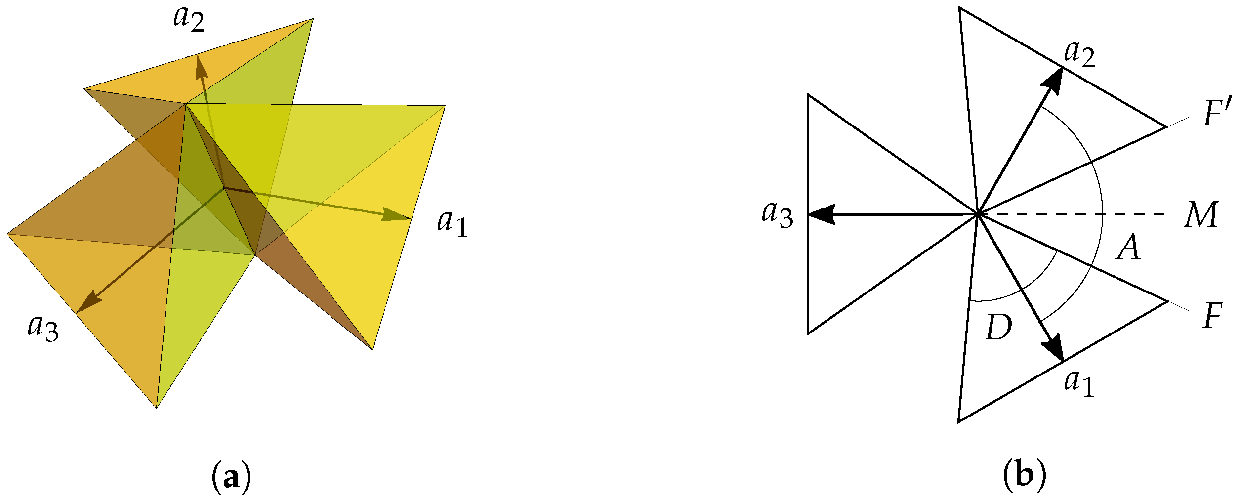
Figure A1.
(a) Edge-sharing group of three tetrahedra, including the from the centre of the shared edge out toward the centres of the respective opposite edges. (The unit vectors are not to scale—the distance between the centres of two opposite edges is not necessarily a unit length.) (b) Overhead view showing the face planes F and that will be rotated into coincidence by the transformation (curve or twist) defined by and . D is the dihedral angle of a tetrahedron and A is the angle between their centres (i.e., between adjacent ).

It is important that each vector makes the same angle A with its neighbours . Furthermore, each tetrahedron has the same dihedral angle D at the shared edge, and we suppose that , so that the tetrahedra do not fill the angular space around the edge, but leave gaps between their faces. (Actually, for our transformations to have the desired effect, it is not strictly necessary that the tetrahedra all be congruent, but only that their dihedral angles at this shared edge be congruent. The value of this angle in our example is determined by the use of regular tetrahedra).
Because all the tetrahedra share a common edge, any two neighbouring ones have adjacent face planes whose line of intersection is that shared edge and whose respective are orthogonal to it. Midway between the two faces we can define a mirror plane M, and together with the two (one in each tetrahedron) this provides the parameters for our transformation, whether the curve or the twist, which will bring those faces into contact. By comparing Figure A1b with Figure 3b where we defined and , we see that
These same angles apply to the faces and mirrors on either side of each tetrahedron, because the tetrahedra centroids are evenly spaced. Thus, will define the same transformation when paired with as with . In this manner, a set of transformations defined by all the and all the reflection planes will close all the gaps and bring all the faces into contact with their neighbouring faces. This can be achieved by either the discrete curve or the twist, with the transformation angle given by Equation (16),
After the transformation, the relative angle between adjacent faces, whether as a dihedral angle or as a twist, will be (Equations (20) and (22))
For regular tetrahedra, the dihedral angle is given by . Arranged about their shared edge in groups of three, four, or five, the respective angles between the are , , and . This leads to the following transformation and face joint angles:
where is the golden ratio satisfying , and .
Appendix A.2. Shared Vertex Configuration, 20 G
In a symmetrically gapped 20-tetrahedron cluster, the tetrahedra are arranged with uniform angular spacing about a shared vertex such that none share any edges (Figure A2). It remains true, however, that any two adjacent tetrahedra have adjacent faces which are symmetric across a mirror plane between them. Although the two faces do not themselves share an edge, the face planes share a common intersection line with the mirror plane (Figure A3), and the curve and twist transformations of Section 4.3 can be applied to bring the faces into contact.
That intersection line between the two face planes contains all points common between them, including therefore the shared vertex. For this case, we define to be the unit vector directed from that vertex out toward the centroid of the ith tetrahedron (hence toward the centre of the tetrahedron’s opposite, outer face, Figure A3b). The in an adjacent tetrahedron will be the reflection of in a vector n lying in the mirror plane between them.
Figure A2.
Vertex-sharing 20-tetrahedron cluster uniformly spaced, with gaps between all faces.
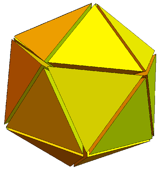
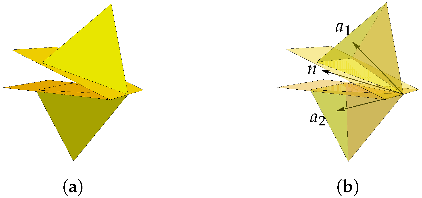
Figure A3.
Example of 2 vertex-sharing tetrahedra with accompanying face planes: (a) shown opaque for visual clarity, particularly where the shared vertex lies on the intersection line of the face planes; and (b) shown partially transparent, so the centroid axes and angle bisector n can be seen.
Figure A3.
Example of 2 vertex-sharing tetrahedra with accompanying face planes: (a) shown opaque for visual clarity, particularly where the shared vertex lies on the intersection line of the face planes; and (b) shown partially transparent, so the centroid axes and angle bisector n can be seen.

Since the tetrahedra are evenly spaced, their 20 centroids lie at the face centres of a regular icosahedron. The angle between adjacent is then supplementary to the icosahedron’s dihedral angle of , or . Furthermore, the angle from an to an adjacent face in its own tetrahedron is complementary to the tetrahedron’s dihedral angle of , so . Equations (16) and (20) then give (using )
These results may also be expressed in terms of the golden ratio , giving
for the vertex-sharing uniformly gapped 20-tetrahedron cluster. These values should be compared with those given in Table 1, which were determined by a sequence of trigonometric calculations. The 20-group considered here contains the same arrangement as the fivefold vertex-sharing configuration in the table; here corresponds to V and B, and corresponds to F and D.
Comparing this vertex-sharing case to the edge-sharing case of fivefold symmetry, note that the transformation angles are different, but the resulting joint angles are the same. This is illustrated geometrically in row five of Table 1, where the vertex-sharing twists are overlaid with scaled images of the edge-sharing twists, showing the same angular configurations.
Appendix A.3. Other Shared Vertex Configurations
If we start with four vertex-sharing tetrahedra, the most symmetric configuration in 3D is to arrange them so their centroids lie at the face centres of a larger tetrahedron. There is then threefold symmetry around an axis, so we call it the threefold vertex-sharing configuration (see the entry in Table 1). The angle between centroid axes is supplementary to the dihedral angle of the large tetrahedron, or ; is the same as before, . Then, we can write for 3-fold symmetry,
For fourfold symmetry, we use two layers of 4 tetrahedra each, with their centroids lying at the face centres of a large octahedron. The angle between centroid axes is supplementary to the octahedron’s dihedral angle of , so , and is still the same. Thus, for fourfold symmetry,
These angles may again be compared with Table 1, for the three- and fourfold cases. (An astute reader will notice a sign difference between the values given here for and those of F and D in Table 1; this is because the values in the table represent interior dihedral angles, while each here is an exterior angle, supplementary to that.)
References
- Sadoc, J.F.; Mosseri, R. Geometric Frustration; Cambridge University Press: Cambridge, UK, 1999. [Google Scholar]
- Martin, T. Shells of atoms. Phys. Rep. 1996, 273, 199–241. [Google Scholar] [CrossRef]
- Fang, F.; Irwin, K.; Kovacs, J.; Sadler, G. Cabinet of curiosities: The interesting geometry of the angle β = arccos((3φ − 1)/4). arXiv, 2013; arXiv:1304.1771. [Google Scholar]
- Fang, F.; Kovacs, J.; Sadler, G.; Irwin, K. An Icosahedral Quasicrystal an Icosahedral Quasicrystal as a Packing of Regular Tetrahedra. ACTA Phys. Pol. A 2014, 126, 458–460. [Google Scholar] [CrossRef]
- Fang, F.; Irwin, K. An Icosahedral Quasicrystal as a Golden Modification of the Icosagrid and its Connection to the E8 Lattice. arXiv, 2015; arXiv:1511.07786. [Google Scholar]
- Fuller, R.B. Synergetics: Explorations in the Geometry of Thinking; Macmillan Publishing Co., Inc.: New York, NY, USA, 1982. [Google Scholar]
- Hestenes, D. Oersted Medal Lecture 2002: Reforming the mathematical language of physics. Am. J. Phys. 2003, 71, 104–121. [Google Scholar] [CrossRef]
- Dorst, L.; Mann, S. Geometric algebra: A computational framework for geometrical applications. IEEE Comput. Graph. Appl. 2002, 22, 24–31. [Google Scholar] [CrossRef]
- Mann, S.; Dorst, L. Geometric algebra: A computational framework for geometrical applications. 2. IEEE Comput. Graph. Appl. 2002, 22, 58–67. [Google Scholar] [CrossRef]
- Doran, C.; Lasenby, A. Geometric Algebra for Physicists; Cambridge University Press: Cambridge, UK, 2003. [Google Scholar]
- Dorst, L.; Fontijne, D.; Mann, S. Geometric Algebra for Computer Science: An Object-Oriented Approach to Geometry; Morgan Kaufmann Publishers Inc.: Amsterdam, The Netherlands, 2009. [Google Scholar]
- Lounesto, P. Clifford Algebras and Spinors, 2th ed.; Number 286 in London Mathematical Society Leture Note Series; Cambridge University Press: Cambridge, UK, 2001. [Google Scholar]
- Elser, V.; Sloane, N.J.A. A highly symmetric four-dimensional quasicrystal. J. Phys. A 1987, 20, 6161–6168. [Google Scholar] [CrossRef]
Figure 1.
Images of: (a) edge-sharing; and (b) vertex sharing local tetrahedral clusters, which fail to locally fill space.
Figure 1.
Images of: (a) edge-sharing; and (b) vertex sharing local tetrahedral clusters, which fail to locally fill space.
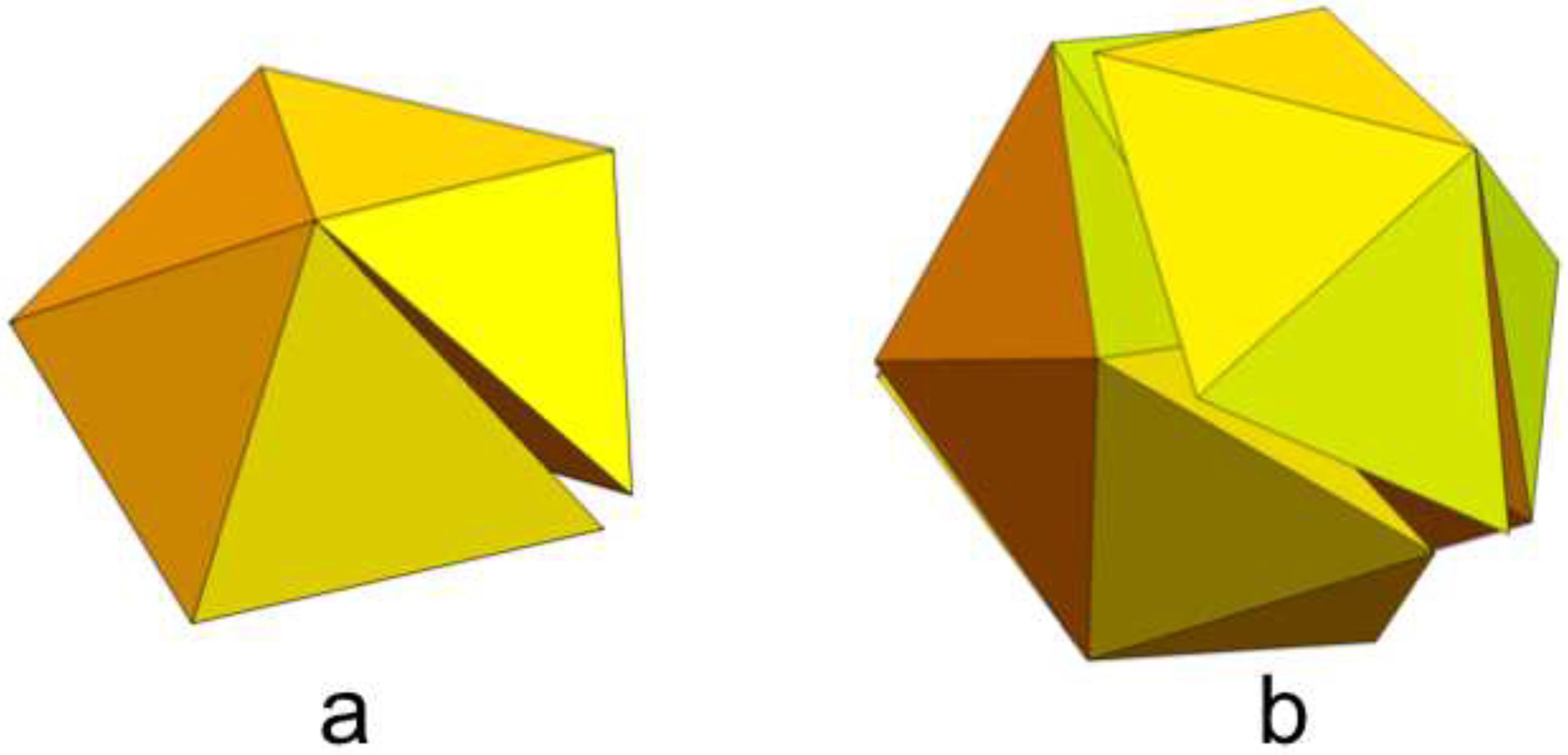
Figure 2.
Symmetric arrangements of a 20-tetrahedron vertex sharing cluster: (a) with open gaps; and then with gaps closed by: (b) discrete curvature; (c) distortion; and (d) twisting. (e,f) The 2D analogue of the transition from gaps to discrete curvature and then to distortion.
Figure 2.
Symmetric arrangements of a 20-tetrahedron vertex sharing cluster: (a) with open gaps; and then with gaps closed by: (b) discrete curvature; (c) distortion; and (d) twisting. (e,f) The 2D analogue of the transition from gaps to discrete curvature and then to distortion.

Figure 3.
Face planes F and symmetric across a mirror plane M, shown (a) obliquely and (b) directly from the direction. They share a common vector h, and have normals f and . The plane normal to h is H, which contains a number of auxiliary vectors. For visual clarity, the bivectors are shown enlarged, but are understood to have unit magnitude.

Figure 4.
The discrete curvature transformation, shown in the 3-space of : (a) the initial configuration; and (b) both the initial and the final state. Shaded planar segments represent bivectors H and before (blue) and after (red) the transformation. Vectors g and rotate in planes parallel to and , respectively, until they meet in the plane, perpendicular to m. Vector a also rotates up to , so between and projects down to between a and n.
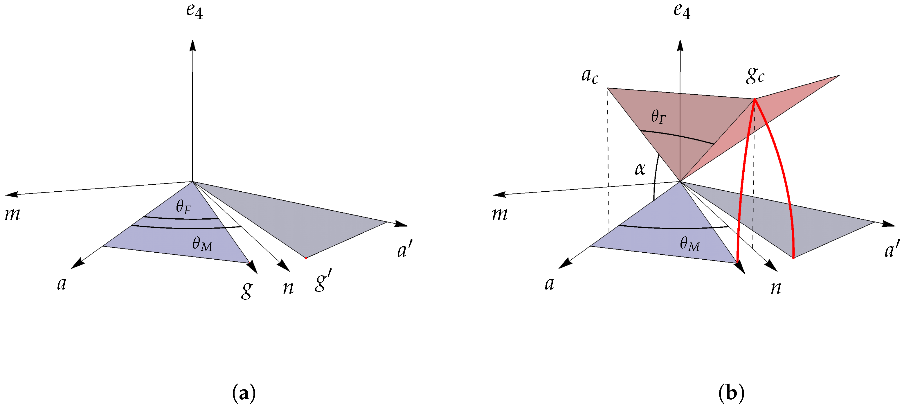
Figure 5.
The twist transformation, in the 3-space of . Bivectors F and are shown: (a) in the initial state; and (b) in the final state, where they are equal, having been rotated clockwise around a and , respectively, until meeting in , which contains n. Their normals f and also rotate around a and , to where they meet in the plane, perpendicular to n. This exactly matches the behavior of g and in Figure 4 above.

Figure 6.
Further illustration of the twist transformation, in the: (a) initial; and (b) final states. Bivectors F and with a dihedral angle of rotate around a. Vector g is rotated around a down to , whereupon between n and a projects in to between and a. Within the H plane the effective dihedral angle (determined by its intersections with and ) has expanded from to .


Table 1.
Properties of three different types of local tetrahedral clusters and their corresponding 4D polyhedra. Symmetrically arranged configurations with gaps are shown in Row 1 (edge sharing) and Row 3 (vertex sharing). Corresponding twisted configurations are shown in Rows 2 and 4. Rows 5 and 6 show overlays of various twisted configurations. In the last two rows note that, for each column, and . The symbol is used for the golden ratio, See the Supplementary Materials for dynamical versions of some images.
| Cluster Types | Threefold | Fourfold | Fivefold |
|---|---|---|---|
| Evenly spaced edge-sharing |  |  |  |
| Twisted edge-sharing |  |  |  |
| Evenly spaced vertex-sharing |  |  |  |
| Twisted vertex-sharing |  |  |  |
| Twisted vertex-sharing, overlaid with twisted edge-sharing, scaled for face matching |  |  |  |
| Twisted vertex-sharing, overlaid with twisted vertex-sharing 20G |  |  |  |
| Transformation angles and joint angles for twist | |||
| Vertex cap of the 4D polytope | 5-cell | 16-cell | 600-cell |
© 2018 by the authors. Licensee MDPI, Basel, Switzerland. This article is an open access article distributed under the terms and conditions of the Creative Commons Attribution (CC BY) license (http://creativecommons.org/licenses/by/4.0/).
Share and Cite
MDPI and ACS Style
Fang, F.; Clawson, R.; Irwin, K. Closing Gaps in Geometrically Frustrated Symmetric Clusters: Local Equivalence between Discrete Curvature and Twist Transformations. Mathematics 2018, 6, 89. https://doi.org/10.3390/math6060089
AMA Style
Fang F, Clawson R, Irwin K. Closing Gaps in Geometrically Frustrated Symmetric Clusters: Local Equivalence between Discrete Curvature and Twist Transformations. Mathematics. 2018; 6(6):89. https://doi.org/10.3390/math6060089
Chicago/Turabian StyleFang, Fang, Richard Clawson, and Klee Irwin. 2018. "Closing Gaps in Geometrically Frustrated Symmetric Clusters: Local Equivalence between Discrete Curvature and Twist Transformations" Mathematics 6, no. 6: 89. https://doi.org/10.3390/math6060089
Note that from the first issue of 2016, this journal uses article numbers instead of page numbers. See further details here.