The “Lévy or Diffusion” Controversy: How Important Is the Movement Pattern in the Context of Trapping?

Abstract

Many empirical and theoretical studies indicate that Brownian motion and diffusion models as its mean field counterpart provide appropriate modeling techniques for individual insect movement. However, this traditional approach has been challenged, and conflicting evidence suggests that an alternative movement pattern such as Lévy walks can provide a better description. Lévy walks differ from Brownian motion since they allow for a higher frequency of large steps, resulting in a faster movement. Identification of the ‘correct’ movement model that would consistently provide the best fit for movement data is challenging and has become a highly controversial issue. In this paper, we show that this controversy may be superficial rather than real if the issue is considered in the context of trapping or, more generally, survival probabilities. In particular, we show that almost identical trap counts are reproduced for inherently different movement models (such as the Brownian motion and the Lévy walk) under certain conditions of equivalence. This apparently suggests that the whole ‘Levy or diffusion’ debate is rather senseless unless it is placed into a specific ecological context, e.g., pest monitoring programs.

1. Introduction

Pests form a significant threat to agricultural ecosystems worldwide, and therefore, effective and reliable monitoring is required to ease the decision making process for intervention. In agro-ecosystems, monitoring is an essential component of integrated pest management programs (IPM) [1,2], where a control action is implemented if necessary. If the population abundance exceeds a certain predefined threshold level, and given that resource effort and expense is readily available, then intervention becomes imminent. Usually, the control action takes the form of pesticide application, which has many negative implications, such as environmental damage in the form of air, soil and water pollution. Such human-induced pressures on the environment often contribute towards bio-diversity loss and affect the functioning of ecosystems [3,4,5]. Other major drawbacks, which are not necessarily related, include cancer-related diseases for those handling such chemicals [6,7], increased consumer costs [8], poor efficiency in reaching targeted pests [9], pest resistance to regular use [10] and lethal effects on natural enemies [11], possibly leading to a resurgence of the pest population or a secondary pest to emerge. Therefore, in order to avoid unnecessary pesticide application or the risk of triggering pest outbreaks, accurate evaluation of population abundance is key [12]. Traps are usually installed in the field under controlled experimental conditions as a means to estimate population abundance [13,14,15]. They are then exposed for the duration of study, insects are caught, traps are normally emptied at regular intervals and the total number that falls into the trap is counted and forms the trap counts. It is precisely these counts that are converted to the pest population density at trap locations and then used to estimate the total pest population size [16,17].

A major ecological challenge is to develop relevant theoretical and mathematical models that can explain patterns and observations obtained from field data [18,19,20]. This is primarily due to the fact that inherent complexity found in the behavior of animals can be difficult to incorporate. However, insects and some invertebrates are easier to model since they have been thought of as non-cognitive. In the case of either single or multiple traps in the same field, individual insect movement can be modeled successfully using a random walk framework [12]. The earliest attempts were based on Brownian motion, which provided a framework to characterize patterns of movement with broad applications to conservation [21,22], biological invasions [23,24,25] and, in particular, insect pest monitoring [12,26,27,28]. Theoretical arguments supported by empirical observations suggest that individuals with limited sensory capabilities tend to follow a Brownian movement pattern, more so at large temporal and spatial scales [29,30,31,32,33,34]. The corresponding mean field counterpart describes the spatial-temporal population dynamics, which is governed by the diffusion equation [12,27,28,35]. Recently, both Brownian motion (BM) and the diffusion model have been often criticized and deemed to be oversimplified descriptions [36]. Other revised models have attempted to account for possible intermittent stop-start movement [37] or inherent intensive/extensive behavioral changes [38]. Simultaneously, there are also other studies with growing empirical evidence that support an alternative description, which postulates that animal movement can exhibit Lévy walking behavior [39,40]. Lévy walks (LW) are differentiated from Brownian movement, since they allow for arbitrarily large steps, that is the probability of executing a larger step is much higher; which results in a faster movement pattern altogether [26,27,41,42].

The usage of the terms Lévy walks or Lévy flights can vary between disciplines. In the physical sciences, a clear distinction is made, but in the ecological literature, the terminology is often interchanged [43]. Some have stressed the crucial distinction between this [44], and others have taken a more relaxed approach [40]. Lévy flights allow for arbitrarily large steps, which can theoretically result in infinite velocities; which is an unphysical/unrealistic phenomenon. On the other hand, Lévy walks ensure that steps are randomly drawn such that the velocity is constant, or nearly so. In order to avoid confusion, we will use Lévy walks as a reference to a random walk whose step distribution has the property of heavy power-law tails, although technically, this is a Lévy flight (see later Section 4.1 for more details). Note that subsequent results and analysis within this study therefore apply indirectly to Lévy walks.

The Lévy or diffusion controversy has arisen from ongoing debates that provide pro and con arguments for each description [42]. Some cases that provide promising evidence for Lévy-type movement [45] have been later classified as Brownian [41] and then have been reclassified as Lévy afterwards [46]. The confusion arises partly due to different studies providing mixed and often conflicting messages. For example, the movement pattern can switch from Brownian to Lévy in a context-specific scenario where resources are scarce [47]. In another study, Lévy-type characteristics can emerge as a consequence of the fundamental observation that individuals of the same species are non-identical [48]. It is also possible that the underlying movement pattern can be misidentified, since variation in the individual walking behavior of diffusive insects can create the impression of a Lévy flight [49]. Furthermore, composite correlated random walks can produce similar movement patterns as Lévy walks; therefore, current methods fail to reliably differentiate between these two models (although recent attempts have been made to address this issue [50]). On the other hand, diffusive properties can appear for a population of Lévy walking individuals due to strong interactions, e.g., if movement is stopped when individuals encounter each other [51]. Even more recently, the diffusion and Brownian framework has been revisited and shown to be in excellent agreement with field data [28]. In either case, it is still unclear which type of movement is adopted by insects, what conditions can alter the pattern and which mathematical framework is most efficient; hence, the controversy persists.

The idea of using a modified diffusion model as an equivalent framework for Lévy walking individuals was first introduced by Ahmed [35] and later further developed [26,27]. In particular, it was demonstrated that in the context of pest monitoring, trap count patterns could be reproduced when comparing a type of Lévy walk to time-dependent diffusion. Further discussions have highlighted that the ecological basis behind incorporating time-dependent diffusion is not clearly understood and how this is linked to the type of mechanisms [26,52,53]. Our study has been instigated by these fruitful discussions leading to an extension to the previous study by Ahmed and Petrovskii [27]. Our aim is two-fold; that is to propose a diffusion model that consists of parameters that are of ecological significance and can be interpreted with reference to the diffusive properties; also, to investigate if trap counts can be effectively reproduced for a broader class of Lévy walks using diffusion. If so, we question the relative importance of identifying the underlying movement pattern. From a cost perspective, it may make sense to concentrate more on the geometry and design of the experiment rather than the particular movement model.

2. BM vs. LW: Equivalence I

2.1. Brownian Motion

Individual-based models provide a complementary cost-effective methodology to field experiments and can be used to simulate movement and analyze trap counts [12,18,54]. The idea is to replicate these experiments through a virtual environment where supplementary and even alternative information is sought [55]. In the specific case of low-density populations, the magnitude of stochastic fluctuations can be quite large, and an individual-based modeling framework can be particularly useful to describe the movement dynamics, i.e., if dangerous pests are present. Note that movement patterns of the Lévy-type have not been identified in field studies for insects, and therefore, our motivation is from a theoretical viewpoint. Our interest is primarily based on understanding the underlying mechanisms that govern movement; it is sufficient to focus on a 1D conceptual scenario. Despite the fact that this case is hardly realistic in terms of modeling movement in a real field setting, however it does provide a theoretical background for the more realistic 2D case [56]. Furthermore, any unnecessary additional complexity that would arise due to the effects of trap and field geometries is then avoided.

The basic idea in 2D is to model walking or crawling insect movement along a continuous curvilinear path, which can be mapped to a broken line with the position recorded at discrete times [18]. In mathematical terms, the 1D analogue over unbounded space for a population of N individuals records the position $X_i^{\left(n\right)}$ of the n-th individual at time t, which is discretized as $t_i=\{t_0=0,t_1,t_2,\cdots ,t_S=T\}$, $i=0,1,\cdots ,S,n=1,2,\cdots ,N$, so that $X_i^{\left(n\right)}=X^{\left(n\right)}\left(t_i\right)$. Here, the script $\left(n\right)$ is included to differentiate between movement tracks of different individuals of the same insect. We assume that positions are recorded at regular intervals with constant time increment:

$$\Delta t=t_i-t_{i-1}=\frac{T}{S},$$

where the first observation is recorded at time $t=0$ with the total number of steps S and total time $t_S=T$. Each individual moves from position $X_{i-1}^{\left(n\right)}$ to $X_i^{\left(n\right)}$ with step length:

$$l_i^{\left(n\right)}=|X_i^{\left(n\right)}-X_{i-1}^{\left(n\right)}|$$

and velocity:

$$v_i^{\left(n\right)}=\frac{|X_i^{\left(n\right)}-X_{i-1}^{\left(n\right)}|}{\Delta t}$$

defined over each step. The n-th individual placed at some position $X_i^{\left(n\right)}$ can move either to the right or to the left with resulting position $X_{i+1}^{\left(n\right)}$. Assuming that each subsequent step is completely random 1 and generated according to a predefined probability distribution $\varphi \left(\xi \right)$, then each further position can be determined by:

$$X_{i+1}^{\left(n\right)}=X_i^{\left(n\right)}+\xi ,i=0,1,\cdots ,S,n=1,2,\cdots ,N,$$

(1)

where $\xi$ is a random variable. Trap counts can then be obtained if the individuals that fall within a well-pre-defined region are removed from the system at regular intervals and counted [12,35].

Generally, animal movement is anisotropic due to the mere fact that animals have a front and rear end [57], resulting in a correlated random walk [30]. For simpler movement modes, such as that of insects, we can assume that the walk is uncorrelated and the direction of movement is completely independent of previous directions. Each position is then solely dependent on the previous location, and therefore essentially Markovian [58,59]. Under this assumption, the resulting movement is isotropic, and there is no preferential direction, i.e., no advection or drift of any kind; which can arise in the presence of an attractant. In relation to the step distribution, $\varphi \left(\xi \right)$ is a symmetric probability density function (pdf) with zero mean, that is $\varphi \left(\xi \right)=\varphi (-\xi )$. In the case of Brownian motion, the corresponding pdf is normal, which reads:

$${\varphi }_n\left(\xi \right)=\frac{1}{\sigma \sqrt{2\pi }}exp\left(-\frac{{\xi }^2}{2{\sigma }^2}\right)$$

(2)

with scale parameter $\sigma$, which can possibly be dependent on time (the subscript n refers to normal). Alternatively, we write $\xi \sim \mathbf{N}(0,{\sigma }^2)$, which denotes that $\xi$ is randomly drawn from a normal distribution with mean zero and variance ${\sigma }^2$. In realistic ecological applications, many insects are released into the field instead of a single individual. Using the 1D scenario as a baseline case, the corresponding analogy is to initially distribute N individuals along a finite spatial interval $x\in (0,L)$. Common release methods used in trap count studies are either of two types; that is uniform or a point source. In the uniform case, we prescribe the initial position as $X_0^{\left(n\right)}\sim U(0,L)$, where $U(a,b)$ denotes the uniform distribution over the interval $a<x<b$. For a point source, we have $X_0^{\left(n\right)}=\tilde{x}$ for all $n=1,2,\cdots ,N$ at $t=0$ with $x=\tilde{x}$ as the centralized location of the release point. The resulting movement pattern is then completely determined by the type of initial condition and step distribution $\varphi \left(\xi \right)$. Note that the population distribution essentially becomes uniform for larger times, and therefore, identical trap counts are obtained irrespective of the type of initial distribution. This effect is realized due to the inherent random movement of individuals in the field. For more detailed information on how the shape of the trap count profile is affected by the type of initial condition, the reader is redirected to [35]. Generally, in most field applications, a uniform initial population distribution can be reasonably assumed. Even in the case when the true release distribution is characterized by multiple point source releases, the effect on trap count variation is somewhat minimal [28]. Henceforth, all simulations in this paper adopt the uniform distribution as an initial condition.

To describe the individual-based model fully, boundary conditions are enforced and defined as follows: an impermeable stop-go ‘sticky’-type boundary is installed at the external boundary at $x=L$ [60], such that at any instant in time, if the individual position exceeds this boundary, that is if $X_i^{\left(n\right)}>L$, then it remains at location $x=L$. The next position in the process is determined purely by (1), and the individual continues to interplay with the dynamics of the system provided $0<X_{i+1}^{\left(n\right)}<L$ at the next step; otherwise, it either remains at the external boundary, if $X_{i+1}^{\left(n\right)}\ge L$ or is deemed to be trapped if $X_{i+1}^{\left(n\right)}<0$. The trap boundary at $x=0$ introduces a perturbation to the movement and is incorporated in the following way: if $X_i^{\left(n\right)}<0$ at any instant in time, then the individual is removed from the system and the total trap count increases by one, functioning as an absorbing boundary. Cumulative trap counts $J_t$ are obtained at each step over discrete times $t=i\Delta t$, resulting in a stochastic trap count trajectory. It may be important to mention that the choice of time step $\Delta t$ has some significance, since it is known that time scale invariance is lost in the presence of an absorbing and/or stop-go boundary, possibly leading to noticeable differences in trap count recordings [60]. Therefore, $\Delta t$ is chosen small enough so that trap counts are in line with counts obtained using alternative methods, such as the mean field analytic or numerical solutions (see Section 3 and Appendix A for details). Furthermore, at the same time, $\Delta t$ is chosen to be sufficiently large, so that the assumption that subsequent steps are uncorrelated is feasible [12,31].

2.2. Condition of Equivalence

In many ecological applications (such as, for instance, conservation and monitoring), it is important to know the probability that a given animal will remain inside a certain domain or area. Since the movement is described by the probability distribution function (pdf) $\varphi \left(\xi \right)$, one can expect that the probability of remaining inside the domain depends on the properties of $\varphi$, in particular on its rate of decay at large distances.

We first consider the case where $\varphi \left(\xi \right)$ is fat-tailed, $\varphi \left(\xi \right)\sim {\left|\xi \right|}^{-(\alpha +1)}$ with $0<\alpha <2$, which is the characteristic exponent for Lévy walks (see Section 4.1 for more details later). We focus on the special case $\alpha =1$ as it is thought, based both on observations of movement patterns [61,62] and on some evolutionary argument [51], to be ecologically the most relevant. In this case, the pdf for the Lévy walk is described by the Cauchy distribution:

$${\varphi }_c\left(x;\gamma \right)=\frac{\gamma }{\pi }\frac{1}{x^2+{\gamma }^2},$$

(3)

where $\gamma$ is a scale parameter and the subscript c refers to Cauchy.

In the case that at $t=0$, the animal is at $x=0$, Function (3) gives the probability density of its position after one step. It is straightforward to see that the pdf of the animal position after i steps, i.e., at time $t_i=i\Delta t$, is given by the same distribution, but with a re-scaled value of the parameter $\gamma$, that is:

$${\varphi }_c\left(x;i\gamma \right)=\frac{i\gamma }{\pi }\frac{1}{x^2+{\left(i\gamma \right)}^2}.$$

(4)

From Equation (4), we may define a symmetric interval of interest $x_i\left(\gamma ,ϵ\right)$, such that the integral in this interval is always equal to a certain quantity $ϵ$,

$${\int }_{-x_i}^{x_i}{\varphi }_c\left(x;i\gamma \right)dx=ϵ,$$

(5)

and determine the limits of this interval as a function of the parameters of the process and the arbitrary probability $ϵ$:

$$x_i\left(\gamma ,ϵ\right)=i\gamma tan\left(\frac{\pi ϵ}{2}\right).$$

(6)

Our goal is to obtain an alternative stochastic process, composed by the sum of random variables from the Gaussian family, which may be comparable to this one in the sense that it replicates the same probability $ϵ$ over the interval of interest (e.g., see [28]). To do that, we will consider the sum $\overline{Y}=Y_1+Y_2+\cdots +Y_i$ of normally-distributed random variables, defined by the pdf:

$${\varphi }_n\left(y;{\Delta }_i\right)=\frac{1}{{\Delta }_i\sqrt{2\pi }}exp\left(-\frac{y^2}{2{\Delta }_i^2}\right),$$

(7)

where the variance ${\Delta }_i^2$ is just the sum of the variances from each random variable $Y_k$,

$${\Delta }_i^2=\sum _{k=1}^i{\sigma }_k^2.$$

(8)

As the relation between the two process is obtained by equating the integrals on the same domain $\left[-x_i,x_i\right]$, we may compute the probability $ϵ$ over the Gaussian process using Equation (7),

$${\int }_{-x_i}^{x_i}{\varphi }_n\left(y;{\Delta }_i\right)dy=\mathrm{erf}\left(\frac{x_i}{{\Delta }_i\sqrt{2}}\right)=ϵ,$$

(9)

and introducing the inverse error function as $\Phi \left(·\right)\equiv {\mathrm{erf}}^{-1}\left(·\right)$ (see footnote2), we relate the two processes by the following relation:

$${\Delta }_i^2\left(\gamma ,ϵ\right)=\frac{x_i\left(\gamma ,ϵ\right)}{2{\Phi }^2\left(ϵ\right)}=\frac{i^2{\gamma }^2{tan}^2\left(\frac{\pi ϵ}{2}\right)}{2{\Phi }^2\left(ϵ\right)}.$$

(10)

In order to determine the behavior of the increments ${\sigma }_k^2\left(\gamma ,ϵ\right)$, i.e., the variance of each additional Gaussian variable required to be comparable to the original Cauchy process, we only need to write Equation (8) as:

$${\Delta }_i^2={\sigma }_i^2+{\Delta }_{i-1}^2,$$

(11)

which immediately leads to the expression:

$${\sigma }_i^2\left(\gamma ,ϵ\right)=\frac{\left(2i-1\right){\gamma }^2{tan}^2\left(\frac{\pi ϵ}{2}\right)}{2{\Phi }^2\left(ϵ\right)}.$$

(12)

Now, we recall that i is the time of the movement (measured in steps). From Equation (12), we therefore conclude that the probability $ϵ$ to confine the insect performing the Lévy walk over the spatial domain $-L<x<L$ coincides exactly with the probability of the same event in the case where the insect performs the Brownian motion, provided the variance of the Brownian motion (i.e., essentially, the diffusion coefficient) increases linearly with time, ${\sigma }_t^2\sim 2t$.

3. Time-Dependent Diffusion

Insect movement is inherently more complex in nature, due to the contribution from both external and internal factors. Typical external factors include environmental effects or stimuli, which can be quite challenging to incorporate from a modeling perspective. Since our interest lies in the actual mechanisms at play, we assume homogeneity in the sense that external factors are absent. In terms of the underlying movement mechanisms, examples of internal factors include individual variation, composite and/or intermittent movement or even time-density-dependent diffusive behavior [63,64]. The main challenge is then to develop a coherent model that can include these different processes and accurately describe the population dynamics. Obviously, the issue becomes more difficult if a combination of these features is present. In the context of insect pest monitoring, diffusion models have been shown to provide a good theoretical framework and the means for trap count interpretation [12,27,35]. In particular, time-dependent diffusion provides an adequate description for more complicated behavior, at least where standard diffusion fails [26,27,35,65]. The notion of insect movement with time-dependent diffusivity is not new and has been observed in field studies [19].

The 1D diffusion equation for the population density $u(x,t)$ with time-dependent diffusion coefficient $D=D\left(t\right)$ over the semi-infinite domain $0<x<\infty$, with initial density $u(x,t=0)=u_0\left(x\right)$ and zero density condition $u(x=0,t)=0$ at the trap boundary, reads:

$$\frac{\partial u}{\partial t}=D\left(t\right)\frac{{\partial }^{2}u}{\partial x^2},u(x,t=0)=u_0\left(x\right),u(x=0,t)=0,0<x<\infty ,t>0.$$

(13)

By introducing a change of the time variable:

$$\tau \left(t\right)={\int }_0^{t}D\left(s\right)ds,$$

(14)

the system of equations (13) transforms to:

$$\frac{\partial u}{\partial \tau }=\frac{{\partial }^{2}u}{\partial x^2},u(x,\tau =0)=u_0\left(x\right),u(x=0,\tau )=0,0<x<\infty ,\tau >0.$$

(15)

The general solution [26,27,66] is then given by:

$$u(x,\tau )={\int }_0^{\infty }\left(F(x-x^{\prime },\tau )-F(x+x^{\prime },\tau )\right)u_0\left(x^{\prime }\right)d{x}^{\prime }$$

(16)

where:

$$F(x,\tau )=\frac{1}{\sqrt{4\pi \tau }}exp\left(-\frac{x^2}{4\tau }\right)$$

(17)

is the fundamental solution of the diffusion equation in (15), which reduces to $F(x,t)=\frac{1}{\sqrt{4\pi Dt}}exp\left(-\frac{x^2}{4Dt}\right)$ in the specific case of constant diffusivity. The diffusive flux through the boundary at $x=0$ corresponds to trap counts $j\left(\tau \right)$, which can be determined by Fick’s law, that is $j\left(\tau \right)=-{\left.\frac{\partial u(x,\tau )}{\partial x}\right|}_{x=0}$ with cumulative trap counts $J\left(\tau \right)$ (total flux) given by:

$$J\left(\tau \right)={\int }_0^{\tau }j\left({\tau }^{\prime }\right)d{\tau }^{\prime }={\int }_0^{\infty }{u}_0\left(x^{\prime }\right)\mathrm{erfc}\left(\frac{x^{\prime }}{\sqrt{4\tau }}\right)d{x}^{\prime }$$

(18)

where $\mathrm{erfc}\left(z\right)=1-\frac{2}{\sqrt{\pi }}{\int }_0^{z}exp\left(-z^{\prime 2}\right)d{z}^{\prime }$ is the complimentary error function. Therefore, the total number of trap counts $J\left(t\right)$ for the system (13) in normal time t is given by,

$$J\left(t\right)={\int }_0^{\infty }{u}_0\left(x^{\prime }\right)\mathrm{erfc}\left(\frac{x^{\prime }}{2\sqrt{{\int }_0^{t}D\left(s\right)ds}}\right)d{x}^{\prime }.$$

(19)

In the case of a uniform distribution $u_0\left(x\right)=U_0$, (19) reduces to:

$$J\left(t\right)=2U_0\sqrt{\frac{1}{\pi }{\int }_0^{t}D\left(s\right)ds}$$

(20)

with:

$$J\left(t\right)=2U_0\sqrt{\frac{Dt}{\pi }}$$

(21)

in the special case with constant diffusivity D, corresponding to standard diffusion.

Equivalence of Trap Counts: Brownian Motion vs. Diffusion in a Semi-Bounded Space

For the diffusion Equation (15), the mean location and mean squared displacement (MSD) are useful statistics that characterize the movement,

$$〈x\left(\tau \right)〉={\int }_{-\infty }^{\infty }xF(x,\tau )dx=0,〈x^2\left(\tau \right)〉={\int }_{-\infty }^{\infty }{x}^{2}F(x,\tau )dx=2\tau ,$$

(22)

where $F(x,\tau )$ is defined by (17). It is well known that diffusion is the macroscopic description of Brownian motion [67], where the MSD is equal to the variance of the step distribution $\varphi \left(\xi \right)$,

$$〈x^2\left(\tau \right)〉=\mathbb{E}\left({\xi }^2\right).$$

(23)

From this, we obtain a link between the scale parameter in (2) and the diffusion coefficient,

$${\sigma }^2\left(t\right)=2\tau =2{\int }_0^{t}D\left(s\right)ds.$$

(24)

For a discrete time model, one can expect that this remains valid, at least approximately, for a small, but finite value of $\Delta t$, that is:

$${\sigma }^2\left(t\right)\approx 2D\left(t\right)\Delta t.$$

(25)

In the case of standard diffusion, the MSD grows linearly with time and is related to the scale parameter by:

$${\sigma }^2\left(t\right)=2Dt,$$

(26)

which is known as the hallmark of Brownian motion [12,18,68]. More generally, for anomalous diffusion, the MSD grows according to some power law relationship:

$$〈x^2\left(t\right)〉\sim t^{2H},$$

(27)

where H is the Hurst exponent. Here, $H=\frac{1}{2}$ corresponds to standard diffusion (26), $\frac{1}{2}<H<1$ corresponds to super-diffusion and $H=1$ corresponds to ballistic or wavelike motion. A full comprehensive summary of movement properties with reference to H can be found in [59].

To demonstrate equivalence between Brownian motion and an anomalous diffusion model, consider as a baseline case:

$$D\left(t\right)=D_0+D_1{t}^{2H-1},H\ge \frac{1}{2}$$

(28)

where $D_0$ is the initial diffusivity and $D_1$ controls the effect of time dependency for a larger time. This structure is chosen as an example, so that the scale parameter (24) is in accordance with (27), i.e.,

$${\sigma }^2\left(t\right)=2{\int }_0^t\left(D_0+D_1{s}^{2H-1}\right)ds=2D_{0}t+\frac{D_1}{H}{t}^{2H}\sim t^{2H}\mathrm{provided}H\ge \frac{1}{2}.$$

(29)

The analytical solution for the model with an initial uniform distribution can be derived from (20), which reads:

$$J\left(t\right)=2U_0\sqrt{\frac{D_{0}t}{\pi }}{\left(1+\frac{D_1}{2D_{0}H}{t}^{2H-1}\right)}^{\frac{1}{2}}$$

(30)

and approximates the flux for constant diffusion (21) for small time.

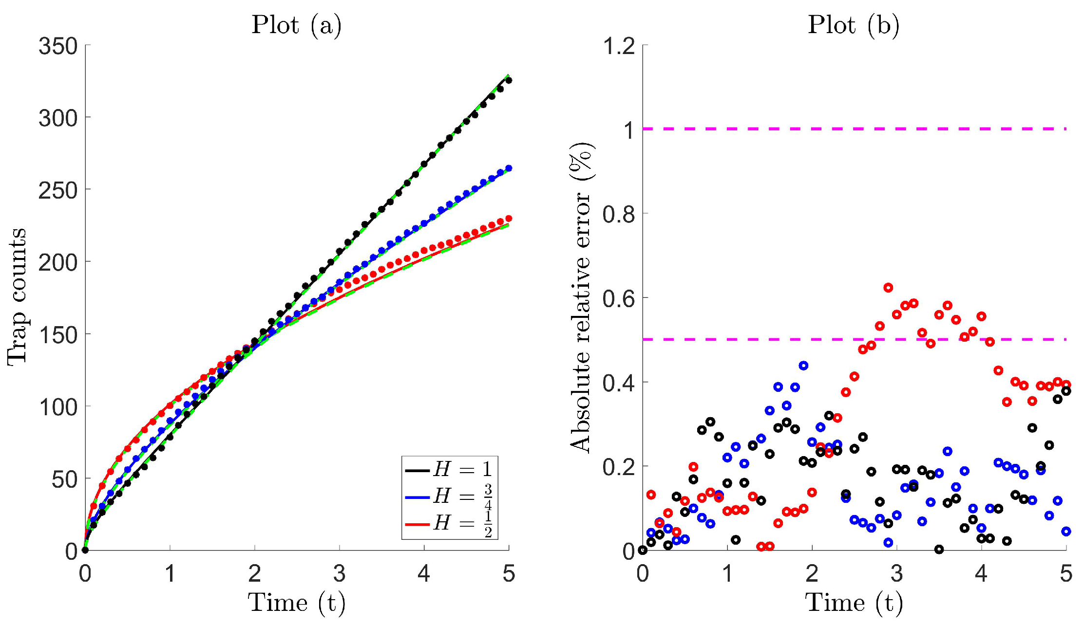
In Figure 1, Plot (a), we find that there is almost identical agreement between trap counts obtained from the Brownian individual-based model and the mean field diffusion model, as expected from theory. More specifically, it is shown here that the diffusive flux can be used to reproduce trap count patterns for standard diffusion $H=\frac{1}{2}$, super diffusion $H=\frac{3}{4}$ and ballistic movement $H=1$, to a high level of accuracy. Intuitively, we expect that this holds for diffusion coefficients that have a more complicated time-dependency. The diffusion coefficient consists of three unknown parameters, namely $D_0,D_1$ and H. In terms of usage, if initial diffusivity can be measured through experiments, then other parameters can be estimated using the tools outlined in [27], i.e., by approximating the flux rate in the limit $t\to 0$ and relating it to the expected number of individuals trapped after one time step. Note that, since an analytical solution cannot be obtained for the diffusion model (15) over a finite domain, the numerical solution is also shown for consistency. See Appendix A for details on the explicit finite difference scheme used and how the flux is computed at the trap boundary.

We introduce the average absolute error $\overline{A}$ as a means to quantify the discrepancy between the models. Although advanced statistical tools exist to measure differences between stochastic and deterministic processes, for our purposes, this simple statistical metric will suffice and will later prove to be effective. The absolute error (relative to the total population) evaluated at discrete times $t=hk$ is defined by,

$$A\left(t_k\right)=\frac{|\mathrm{Diffusive}\mathrm{flux}-\mathrm{Trap}\mathrm{counts}|}{\mathrm{Total}\mathrm{population}}=\frac{|J\left(hk\right)-J_{hk}|}{N},k=0,1,2,\cdots ,K$$

(31)

with time increment h and total time $T=hK$. The errors are then averaged over $(K+1)$ differences,

$$\overline{A}\left(t_k\right)=\frac{1}{N(K+1)}\sum _{k=0}^K|J\left(hk\right)-J_{hk}|.$$

(32)

Plot (b) illustrates the discrepancy using the absolute error, which lies within 0.6 and 0.7% of all total trap counts. Theoretically, the Brownian and corresponding diffusion model are equivalent, and the errors can be dismissed as somewhat negligible, partly due to the accumulation of small computational errors. We expect this error to tend to zero, with the magnitude of stochastic fluctuations decreasing as $N^{-\frac{1}{2}}$ in the limit $N\to \infty$ [69]. Furthermore, longer time simulations (not shown) demonstrate that the discrepancy increases as the effect of external boundary encounters is realized. Therefore, we require that the finite domain is large enough, that is $\frac{L^2}{D}$ is much larger than the typical characteristic trapping time. The quantified errors in

Table 1. Tabulated values of the average absolute relative error $\overline{A}$ as defined by (32), to compare the fit between the anomalous diffusion model (30) and trap counts obtained from Brownian motion (see Figure 1).

	Standard Diffusion $\mathit{H}=\frac{1}{2}$	Super Diffusion $\mathit{H}=\frac{3}{4}$	Ballistic Diffusion $\mathit{H}=1$
Brownian trap counts	0.306	0.157	0.167

are probably not useful on their own; however, for now, they function as benchmark values, which indicate an extremely good fit; indicating equivalence. As a general rule of thumb, we classify the level of fit as equivalent $0<\overline{A}\le 0.5$, good fit $0.5<\overline{A}\le 1$, moderate fit $1<\overline{A}\le 1.5$ and poor fit $\overline{A}>1.5$. These will be useful later as a point of reference, when comparisons are made between various diffusion models, in an attempt to reproduce Lévy trap count data.

4. BM vs. LW: Equivalence II

4.1. Stable Laws

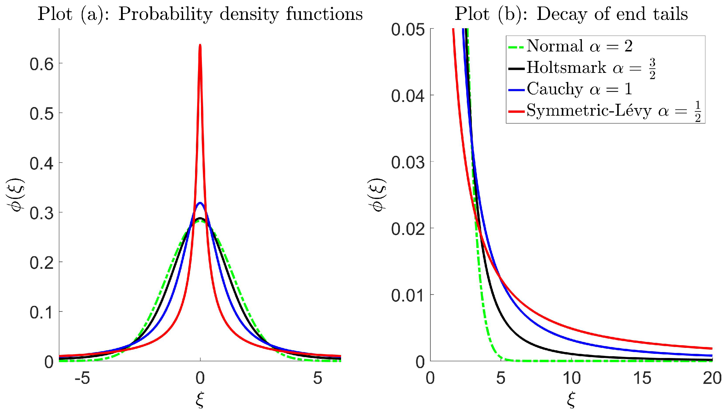
In the case of Brownian motion, the step distribution is normal (2), and the end tails decay exponentially fast (thin tail). A large number of studies has shown that animal movement can follow a more complicated movement pattern where the step distribution decays much more slowly according to some type of inverse power law (heavy or fat tail), known as Lévy walks [32,45,70]. As a result, individuals have a greater chance of executing ‘rare’ large steps, and therefore, the properties of the random walk are altered. The biological consequence is such that the overall movement pattern is faster in comparison to what is typically observed in Brownian motion. Lévy walks can be characterized by Lévy $\alpha$-stable distributions, simply known as stable laws. A distribution is said to be stable if the sum (or, more generally, a linear combination with positive weights) of two independent random variables has the same distribution up to a scaling factor and shift [44,71]. The mechanisms behind the resulting movement are governed by the step distribution, which is completely described using four parameters, namely a tail index $\alpha \in (0,2]$, skewness parameter $\beta \in [-1,1]$, scale parameter $\gamma \in (0,\infty )$ and location parameter $\delta \in \mathbb{R}$. The asymptotic behavior of the end tails is,

$$\varphi \left(\xi \right)\sim {\left|\xi \right|}^{-(\alpha +1)},\xi \to \pm \infty ,$$

(33)

where $\alpha \in (0,2]$ determines the rate at which the tails of the distribution taper off. For $\alpha \le 0$, the distribution cannot be normalized, and therefore, the pdf cannot be defined. For $\alpha \ge 2$, the end tails decay sufficiently fast at large $\left|\xi \right|$, ensuring that all moments exist and the central limit theorem (CLT) applies, that is the probability density of the walker after S steps converges to the normal distribution as $S\to \infty$. The generalized central limit theorem (gCLT) states that the sum of identically-distributed random variables with distributions having inverse power law tails converges to one of the stable laws, of which the normal distribution is a special case. For the range $0<\alpha <2$, the gCLT applies, and the condition on the second moment is relaxed; that is, second moments diverge, and the tails are asymptotically equivalent to a Pareto law. Since their first introduction, usage of stable laws has been overlooked and somewhat neglected, mainly due to difficulties arising from an infinite variance. However, there are now well-developed and readily-available algorithms that can be exploited for simulation runs [72,73], and thus, stable laws are increasingly being considered, particularly in movement ecology [40].

Stable laws can be parametrized in $\mathcal{Z}$ different, but equivalent ways, and currently, there exists at least eleven different variations, which has led to much confusion [74,75]. Each type has an advantage over the others, and the parameter $\mathcal{Z}$ is often chosen based on the purpose of use, i.e., simulation-based studies, data fitting or the study of algebraic/analytic properties. Since our focus is primarily based on obtaining trap counts from simulations, we choose the $\mathcal{Z}=0$ parametrization and henceforth use this setting. We adopt the notation introduced by [71]; that is, the random variable $\xi$ is drawn from the stable distribution:

$$\mathbf{S}(\alpha ,\beta ,\gamma ,\delta ;\mathcal{Z}).$$

Since explicit pdfs are not available for all values of $\alpha \in (0,2]$, the distribution is often described in terms of the characteristic function: the inverse Fourier transform of the pdf,

$$ln\mathbb{E}{e}^{i\omega \xi }=\left\{\begin{array}{cc}\hfill -{\gamma }^{\alpha }{\left|\omega \right|}^{\alpha }\left[1+i\beta tan\frac{\alpha \pi }{2}·\mathrm{sign}\left(\omega \right)·{\left(\right|\gamma \omega |}^{1-\alpha }-1)\right]+i\delta \omega ,& \alpha \ne 1\\ \hfill -\gamma \left|\omega \right|\left[1+\frac{2i\beta }{\pi }·\mathrm{sign}\left(\omega \right)·log\left|\gamma \omega \right|\right]+i\delta \omega ,& \alpha =1\end{array}\right.$$

(34)

For an isotropic random walk, the pdf of the step distribution is symmetrical, and therefore, both the skewness and location parameters are fixed with $\beta =\delta =0$. The resulting distribution is known as an $\alpha$-stable symmetric Lévy distribution, which is then completely characterized solely by the index $\alpha$ and scale parameter $\gamma$. For brevity, we adopt the notation:

$$\mathbf{S}(\alpha ,\beta =0,\gamma ,\delta =0;\mathcal{Z}=0)=\mathbf{S}(\alpha ,\gamma ),$$

where it is understood that all parameters are zero except $\alpha$ and $\gamma$. The resulting characteristic function in (34) reads:

$$\mathbb{E}{e}^{i\omega \xi }=exp\left(-{\gamma }^{\alpha }{\left|\omega \right|}^{\alpha }\right),$$

(35)

which is a useful way to mathematically describe all (symmetric) stable distributions, since a closed form or analytical expression does not exist for all indices $\alpha$, with the exception of the normal $\alpha =2$ and Cauchy $\alpha =1$ cases;

$$\begin{array}{cc}\mathrm{Normal}\xi \sim \mathbf{S}(2,{\gamma }_n)\hfill & \hfill {\varphi }_n\left(\xi \right)=\frac{1}{2{\gamma }_n\sqrt{\pi }}exp\left(-\frac{{\xi }^2}{4{\gamma }_n^2}\right),{\gamma }_n=\frac{\sigma }{\sqrt{2}}\end{array}$$

(36)

$$\begin{array}{cc}\mathrm{Holtsmark}\xi \sim \mathbf{S}\left(\frac{3}{2},{\gamma }_h\right)\hfill & \hfill {\varphi }_h\left(\xi \right)\mathrm{Cannot}\mathrm{be}\mathrm{expressed}\mathrm{in}\mathrm{closed}\mathrm{form}\end{array}$$

(37)

$$\begin{array}{cc}\mathrm{Cauchy}\xi \sim \mathbf{S}(1,{\gamma }_c)\hfill & \hfill {\varphi }_c\left(\xi \right)=\frac{{\gamma }_c}{\pi ({\gamma }_c^2+{\xi }^2)}\end{array}$$

(38)

$$\begin{array}{cc}\mathrm{Symmetric}-\mathrm{L}é\mathrm{vy}\xi \sim \mathbf{S}\left(\frac{1}{2},{\gamma }_l\right)\hfill & \hfill {\varphi }_l\left(\xi \right)\mathrm{Cannot}\mathrm{be}\mathrm{expressed}\mathrm{in}\mathrm{closed}\mathrm{form}\end{array}$$

(39)

where the subscripts $n,h,c,l$ have been included to distinguish between the different distributions. For the normal distribution, $\sigma$ is the standard deviation shown in the step distribution (2), with ${\gamma }_n$ defined in this way due to the choice of parametrization. This relation can be easily derived through the characteristic function (35). Note that, some authors use the term ‘Lévy distribution’ to refer to stable laws; however, more commonly, it refers to $\alpha =\frac{1}{2},\beta =1$, which is a skewed distribution, defined for $\xi \ge 0$ [71]. Since we consider symmetric distributions, i.e., $\beta =0$, we will refer to (39) as the ‘symmetric’-Lévy distribution. In some cases, the pdf can be expressed analytically, even if it cannot be written in closed form, e.g., the Holtsmark distribution (37) can be written using hyper-geometric functions (if symmetric) or the Whittaker function (if skewed). Furthermore, the symmetric-Lévy distribution can be expressed in terms of special functions, such as Fresnel integrals [74]. However, these representations are bulky and not useful in the context of this study.

Figure 2 illustrates pdfs for symmetric stable laws with the decay of end tails characterized by different indices $\alpha =\frac{1}{2},1,\frac{3}{2},2,$ with faster decay rates as $\alpha$ increases and exponential fast decay in the case of the normal distribution.

4.2. Equivalence of Trap Counts: Cauchy Walk vs. Diffusion

Standard diffusion provides an oversimplified description [76], partly due to an underlying assumption that all individuals are identical in terms of their movement capabilities. In reality, this is not entirely true, and it is known that individuals in the field do not possess an equal ability for self-motion. Even in the case of a population of an identical insect species type, distinct traits can significantly affect movement abilities, such as body mass, length of wings or more generally shape and size [77]. To overcome this assumption, modified diffusion models have been successfully introduced. For example, [48] take into account that the diffusion coefficient can vary according to some type of diffusivity distribution function, rather than being constant. As a result, it is shown that by introducing the concept of a statistically-structured population, the fat tails that are inherent in Lévy walks can appear due to the fact that individuals of the same species are non-identical. Therefore, the mechanism of fat tails’ formation in a real population is always present, even if it can sometimes be induced by a mixture of other processes. This is not the only approach that attempts to explain the phenomena of fat tails appearing. We propose an alternative model (see later Section 4.3), where diffusivity varies continuously with time. On an individual level, the interpretation is such that distinct diffusive rates are adopted, and therefore, the model takes into account individual variation. However, at the population level, when rates are aggregated, the movement is governed by time-dependent diffusion.

In Section 3, it was demonstrated that equivalent trap counts can be obtained for Brownian movement using an anomalous diffusion model (30). Here, we test whether this same model can explain trap counts from non-Brownian movement, with particular interest in the level of discrepancy.

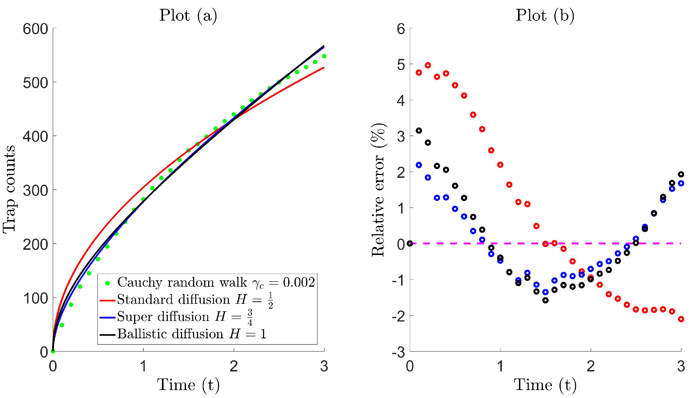
Figure 3, Plot (a), compares trap counts $J_t$ from the Cauchy walk 3 against the diffusive flux $J\left(t\right)$ for exponents; standard diffusion $H=\frac{1}{2}$, super-diffusion $H=\frac{3}{4}$ and ballistic diffusion $H=1$. A non-linear curve fitting tool is used to determine the best-fit parameters $D_0,D_1$ by fitting the analytic solution (30) against trap count recordings in the least squares sense (see

Table B1. Trap count recordings for the cases (a) Holtsmark $S(\alpha =\frac{3}{2},{\gamma }_h)$, (b) Cauchy $S(\alpha =1,{\gamma }_c)$ and (c) symmetric-Lévy $S(\alpha =\frac{1}{2},{\gamma }_l)$, with tail exponent $\alpha$ and scale parameter $\gamma$. Simulation details with all parameter values are given in the caption of Figure 5.

Time $\left(\mathit{t}\right)$	${\mathit{\gamma }}_{\mathit{h}}=0.01$	$0.02$	$0.04$	${\mathit{\gamma }}_{\mathit{c}}=0.0005$	$0.002$	$0.003$	${\mathit{\gamma }}_{\mathit{l}}=1\times {10}^{-6}$	$4\times {10}^{-6}$	$2\times {10}^{-5}$
0.1	54	93.8	188	21.6	48.6	91	32.6	69.4	134.2
0.2	83.2	147.2	283.4	36.4	86.4	147.8	60.6	123.4	241.6
0.3	106.6	195.6	355.2	53.2	120.2	206.2	94	173	324.8
0.4	127.6	235.6	413.8	68.4	145	252.6	123.2	222.2	399.4
0.5	146.2	270.6	466	78.4	171	291.2	147.4	263.6	460.8
0.6	163.2	299.6	510.4	91.6	194.4	328.4	171.6	305	513
0.7	180.6	326.2	551.8	103.8	218.6	364.4	196	340.4	560.
0.8	195.6	351.6	588.8	116.6	240.2	394.8	219.6	376.4	603.
0.9	209.8	376.8	629.6	126	262.6	425.4	238.4	409.6	645.8
1.0	225.6	400.8	661	133.8	282.2	451.6	258	438.2	686.4
1.1	238.2	421.8	689.6	143.2	302.6	476	279	466.2	717.4
1.2	251.4	442.4	715.2	155.4	321.6	498.4	298.6	491.6	746.4
1.3	260.8	460.4	740.6	166.4	335.8	521.2	321.4	513	773.2
1.4	271	482	760.4	175.2	355	545	341.4	536.2	797
1.5	282.6	499	783	184.2	372.6	563.8	358.6	555.2	820.2
1.6	290.6	516.2	804	194.2	384.6	584	374.8	575.8	839
1.7	301	531.4	821.2	204.8	398	600.8	390.2	596	856.8
1.8	311	546.4	836.4	214.2	413	617.4	407.8	612.2	871.2
1.9	323	562.8	851.6	222.6	427	633.8	422.8	632	883
2.0	333.2	574	864	231.8	439.6	652.6	435	648.6	894.8
2.1	342.6	586.2	877.2	333.2	574	864	446.6	668.4	904.6
2.2	350.4	599	888.8	241.8	452.2	669	462	681	912.4
2.3	359.2	609.2	898.8	246.4	465.2	683.8	474.2	694.2	919.4
2.4	369.4	620.2	907.6	254.2	476.6	695.2	488.6	704	928.2
2.5	376.2	631	914.8	263	488.2	708.2	502.6	716.4	934.6
2.6	386.2	645.8	921.8	271.6	499.2	721.2	515	730.4	941.6
2.7	394.4	655.4	928.4	280	509	735.2	525.6	747.4	946.2
2.8	399.4	666.8	934.4	288	518.2	745.8	538	756.4	950.2
2.9	407.6	678.2	938.8	294.2	527.2	757	550	768.2	956.2
3.0	415	686.8	943.8	301.2	536.8	766.8	560.8	779.2	961.2

for the complete list of trap count recordings). Plot (b) illustrates the discrepancy between the trap counts and diffusion model. The relative error is shown (instead of the absolute relative error used previously in Figure 1) to distinguish between the time intervals when trap counts are either over- or under-estimated; here, a positive relative error corresponds to the diffusive flux forming an overestimation, and vice versa.

Table 2. Tabulated values of the average absolute relative error $\overline{A}$ as defined by (32), to compare the fit between the anomalous diffusion model (30) and trap counts obtained from Brownian motion (see Figure 1) and the Cauchy walk (see Figure 3).

	Standard Diffusion $\mathit{H}=\frac{1}{2}$	Super Diffusion $\mathit{H}=\frac{3}{4}$	Ballistic Diffusion $\mathit{H}=1$
Brownian trap counts	0.306	0.157	0.167
Cauchy trap counts	2.035	0.849	1.120

quantifies the fit and compares whether the diffusion model can reproduce trap counts as effectively as what was previously seen in the Brownian case (see Figure 1).

From Figure 3, Plot (b), it is clear that standard diffusion fails to predict trap counts adequately, with a maximum relative error of about 5%. This is expected since standard diffusion corresponds to the random walk model with a normal step distribution whose end tails decay exponentially, unlike the Cauchy distribution. On comparison, Table 2 shows that both super diffusion and ballistic diffusion provide a good/moderate fitting, respectively. Petrovskii et al. [26] demonstrated that in the case of some simple diffusion models, such as linear dependency on time $D\left(t\right)=at+b$ and its variation $D\left(t\right)=at+b{t}^{\frac{1}{3}}$ ($a,b$ constant), both of which constitute ballistic motion, provide a reasonable fit to trap count data. Figure 3 also confirms a reasonable fit for the ballistic case where the relative error lies within approximately 3%; however, still, an evident discrepancy is noticed. Trap counts are much better reproduced by super-diffusion, in this case $H=\frac{3}{4}$ with relative error within approximately 2%. This is somewhat expected, since it is well known that generally, super diffusion has long been acquainted with Lévy walks [43,78]. Despite this promising accuracy, note that the diffusion flux tends to alternate; in the sense that trap counts are overestimated for small time, underestimated for intermediate time and overestimated again on a larger time scale; for both the super diffusive and ballistic case. This phenomenon is also realized for other Hurst exponents in the super-diffusive and ballistic regime (simulations not shown here), even when a variety of scale parameters is considered. Although the accuracy of the matching is somewhat ecologically acceptable in either case, a diffusion coefficient that yields trap counts at a higher level of precision is sought.

In a recent study, Ahmed and Petrovskii [27] demonstrated that the time-dependency of the diffusion coefficient could be inherently more complex than that proposed by anomalous diffusion. Subsequently, a time-dependent diffusion model was developed to provide an alternative framework for a Cauchy walk with the step distribution (38). In particular, passive trap counts were reproduced effectively, and the study indicated that in the case of a Cauchy walk, the problem of trap count interpretation can be addressed with a high precision based on the diffusion equation. However, some drawbacks with this model 4 include, firstly, that the complicated structure of the diffusion coefficient leads to practicality issues, since it is not expressed in closed form. Secondly, the model consists of multiple unknown parameters with little room for interpretation, i.e., the ecological significance of parameters or how they relate to the movement pattern is unclear. Finally, the study is constrained to Cauchy walks, and it is not known whether the diffusion model is effective at predicting trap counts for a broader range of tail indices $\alpha$. With this background, we attempt to address the following: Can trap counts obtained from a system of genuine Lévy walkers be accurately reproduced using the diffusion equation, in particular, with a greater accuracy than what is observed for anomalous diffusion in Figure 3? If so, what is the structure of the diffusion coefficient, and how can the behavior of the resulting diffusion profiles be explained from an ecological viewpoint in relation to any parameters?

4.3. Proposed Diffusion Coefficient

Observations of trap count patterns (such as those typically observed in Figure 3) suggest that the coefficient proposed should consist of some type of growth function $G\left(t\right)$, which should behave as a controlling mechanism for diffusivity on a short and/or intermediate time scale. In addition to this, a suitable decay function should also be introduced to induce a dampening effect to ensure that trap counts are not overestimated for larger times, typically observed when the movement process grows faster than standard diffusion. Intuitively, we propose the following structure:

$$D\left(t\right)=\underset{\begin{array}{c}\mathrm{Initial}\\ \mathrm{diffusivity}\end{array}}{\underbrace{D_0}}+\underset{\begin{array}{c}\mathrm{Growth}\\ \mathrm{function}\end{array}}{\underbrace{G\left(t\right)}}·\underset{\begin{array}{c}\mathrm{Exponential}\\ \mathrm{decay}\end{array}}{\underbrace{e^{-\nu t}}}$$

(40)

with $G\left(0\right)=0$, i.e., growth is zero at $t=0$ so that initial diffusivity is defined as $D\left(0\right)=D_0$, with obvious meaning. Here, the growth function is subject to exponential decay causing the diffusivity to be damped over larger times with damping coefficient $\nu$. Subsequently, the diffusivity returns to an initial state $D_0$ in the large time limit as $t\to \infty ,$ provided the growth function is not faster than exponential growth, that is ${lim}_{t\to \infty }G\left(t\right)e^{-\nu t}=0$. The corresponding diffusive flux for an initial uniform population density $U_0$ across a semi-infinite domain $x>0$ with zero density condition at $x=0$ (described in Section 3) can be derived using (20), which reads:

$$J\left(t\right)=2U_0\sqrt{\frac{D_{0}t}{\pi }+\frac{1}{\pi }{\int }_0^{t}G\left(s\right)e^{-\nu s}ds}.$$

(41)

A number of possible candidates for the growth function exist in the literature, but are often applied to model population dynamics. Examples of such include logistic, Gompertz, von Bertalanffy and generalized or hyper-logistic growth [79]. The simplest of these is the logistic type, and an example of an application is the Rosenzweig and MacArthur [80] model for predator-prey interactions with logistically growing prey. We propose that the growth function $G\left(t\right)$ in (40) grows logistically, as a means to model diffusivity, rather than the typical use of modeling populations, so that:

$$G\left(t\right)=D_{1}t\left(1-\frac{t}{k}\right)$$

(42)

with corresponding diffusion coefficient:

$$D\left(t\right)=D_0+D_{1}t\left(1-\frac{t}{k}\right)e^{-\nu t}.$$

(43)

The movement dynamics are then completely governed by set parameters $\{D_0,D_1,k,\nu \}$, all positive. This growth function is a parabolic function of time, which increases from $G=0$ at time $t=0$, until a maximum $G_{\max }=\frac{1}{4}{D}_{1}k$ is attained at time $t=\frac{k}{2}$, and then decreases until the growth diminishes, i.e., $G=0$ at time $t=k$. The corresponding diffusion coefficient is still valid for negative growth over the interval $k<t<t^{\ast }$ provided $D\left(t\right)>0$, where $t^{\ast }$ is a solution of $ln{D}_1(t^{\ast }-k)-\nu t^{\ast }=ln{D}_{0}k$. For fixed $D_1$, the value of k controls the maximum growth capacity and also determines the instant in time when growth alternates from positive to negative. In the special case, for sufficiently small time with large k, the term $\frac{t}{k}$ in (43) is negligible, and the growth function is approximately linear $G\left(t\right)\approx D_{1}t$, and in the limiting case as $k\to \infty$,

$$G\left(t\right)=D_{1}t$$

(44)

with corresponding diffusion coefficient,

$$D\left(t\right)=D_0+D_{1}t{e}^{-\nu t}$$

(45)

which now depends on three parameters $\{D_0,D_1,\nu \}$. The corresponding diffusive flux can be derived for the logistic model (42) from (41), which results in:

$$\mathrm{Model}1:J\left(t\right)=\frac{2U_0}{\sqrt{\pi }}{\left(D_{0}t+\frac{D_1}{{\nu }^2}\left[1-(1+\nu t)e^{-\nu t}\right]+\frac{D_1}{k{\nu }^3}\left[({\nu }^2{t}^2+2\nu t+2)e^{-\nu t}-2\right]\right)}^{\frac{1}{2}}$$

(46)

and simplifies to:

$$\mathrm{Model}2:J\left(t\right)=\frac{2U_0}{\sqrt{\pi }}{\left(D_{0}t+\frac{D_1}{{\nu }^2}\left[1-(1+\nu t)e^{-\nu t}\right]\right)}^{\frac{1}{2}}$$

(47)

in the reduced linear case (44). Henceforth, we will refer to this as Models 1 and 2, respectively.

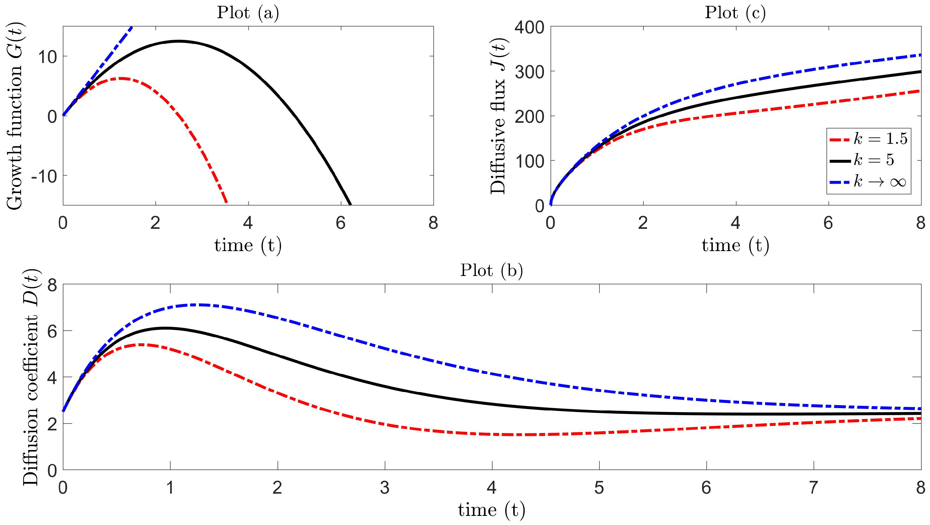
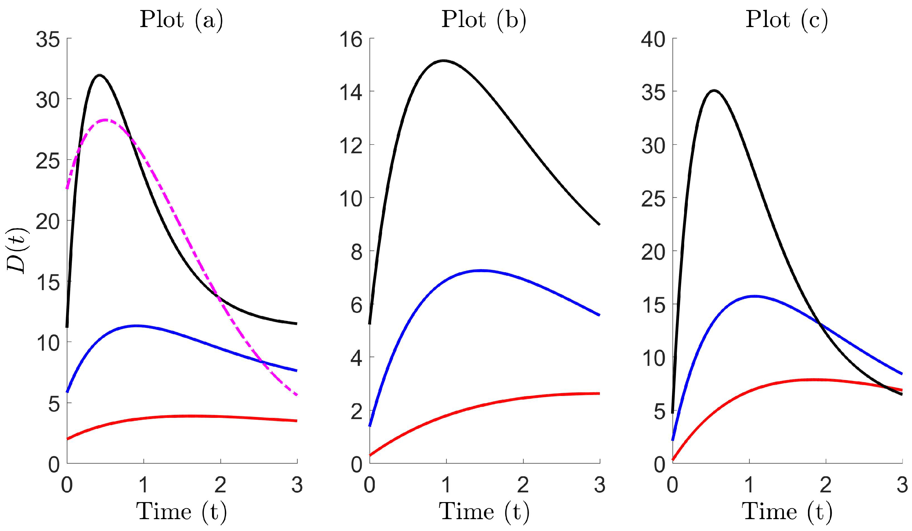
Figure 4, Plot (a), illustrates the logistic growth function as a parabolic profile for different values of k, with linear growth as $k\to \infty$. Figure 4, Plot (b), shows how the diffusion coefficient behaves for particular parameter values. In ecological terms, the mechanistic process is such that insect diffusivity increases from the initial value $D_0$ until maximum diffusivity $D_{\max }$ is attained at time $t=\frac{k}{2}+\frac{1}{\nu }-\frac{k}{2}\sqrt{1+\frac{4}{{\left(k\nu \right)}^2}}$. We presume that this increase in diffusion rate can induce faster movement, which can be comparable (at some level) to the pattern inherent in Lévy walks. Following this, the diffusivity begins to decrease until it reaches a minimum level $D_{\min }$ at time $t=\frac{k}{2}+\frac{1}{\nu }+\frac{k}{2}\sqrt{1+\frac{4}{{\left(k\nu \right)}^2}}$ and then asymptotically approaches the initial state $D_0$ in the large time limit. In the special case of the linear growth function, insect diffusivity reaches $D_{\max }=D_0+\frac{D_1}{e\nu }$ at time $t=\frac{1}{\nu }$ with no subsequent local minimum and the same asymptotic behavior as $t\to \infty$. Figure 4, Plot (c), illustrates the flux for each corresponding diffusion coefficient in Plot (b), and it is precisely these diffusion Models 1 and 2 ((46)–(47)) that will be tested in Section 4.4 against Lévy trap count data.

4.4. Reproducing Lévy Trap Counts Using Diffusion

In this section, we test Models 1 (46) and 2 (47) against Lévy trap count data (see Figure 5 and Table B1). The simulation setting, alongside the initial and boundary conditions, is precisely that which is outlined in Section 2.1, with the difference that the steps $\xi$ are now randomly drawn from those stable laws, defined in ((37)–(39)). Furthermore, the assumptions that the walk is uncorrelated and unbiased in a homogeneous environment still apply. In a system of N individuals executing a Lévy walk, the position of the n-th individual at the $(i+1)$-th step can be described by:

$$X_{i+1}^{\left(n\right)}=X_i^{\left(n\right)}+\xi ,i=0,1,\cdots ,S,n=1,2,\cdots ,N,\xi \sim \mathbf{S}(\alpha ,\gamma ),\alpha \in (0,2).$$

(48)

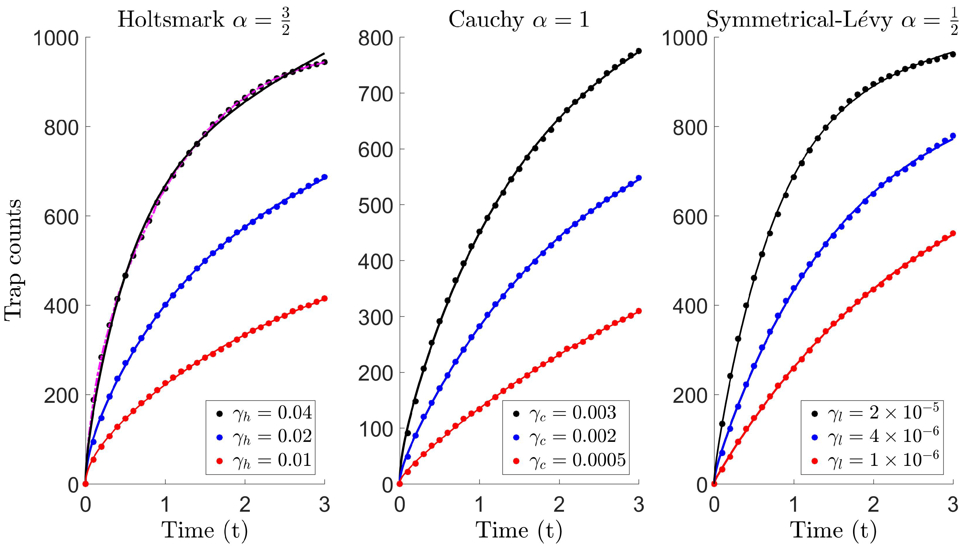
The trap count is expected to grow faster with time, compared to what is usually recorded for Brownian movement. This is due to the frequency of long jumps increasing, and therefore, the contribution from remote parts of the population to the trap count also increases. For our purposes, we simulate trap counts for the tail indices $\alpha =\frac{3}{2},1,\frac{1}{2}$, referring to the Holtsmark (37), Cauchy (38) and symmetric-Lévy (39) distributions, previously introduced in Section 4.1. The movement dynamics are completely governed by the scale parameters ${\gamma }_h,{\gamma }_c,{\gamma }_l$. Although, comparing random walks prior to simulation runs can reveal information on parameter selection [81] (also see Section 2.2), for our purposes, it suffices to arbitrarily select three distinct scale parameters for each case, i.e., ${\gamma }_h=0.01,0.02,0.04$, ${\gamma }_c=0.0005,0.002,0.003$ and ${\gamma }_l=1\times {10}^{-6},4\times {10}^{-6},2\times {10}^{-5}$. Here, parameters are chosen so that trap count data are obtained with a reasonable level of variation (see Table B1). The diffusive flux curves $J\left(t\right)$ given by Model 1 (46) and Model 2 (47) are then fitted (in the least squares sense) against these trap counts using a non-linear curve fitting tool, and the best-fit parameters are estimated, listed in

Table 3. Best-fit parameters using a non-linear curve fitting tool (in the least squares sense) by fitting Model 1 (46) and Model 2 (47) against cumulative trap counts (see Table B1 for the complete list of recordings). The diffusion coefficients in Figure 6 are those plotted with highlighted parameters in the table below.

	${\mathit{D}}_0$	${\mathit{D}}_1$	$\mathit{\nu }$	k	${\mathit{D}}_0$	${\mathit{D}}_1$	$\mathit{\nu }$
${\gamma }_h=$ 0.01	1.974	3.186	0.615	1286.032	1.9745	3.1834	0.6158
0.02	5.798	16.488	1.102	2846.675	5.7984	16.4881	1.1025
0.04	22.552	26.262	0.631	1.235	11.1403	133.0602	2.3539
${\gamma }_c=$ 0.0005	0.286	2.083	0.327	2598.906	0.2861	2.0828	0.3276
0.002	1.374	10.971	0.687	1918.029	1.3743	10.9709	0.6874
0.003	5.218	27.968	1.036	2589.831	5.2184	27.9676	1.0365
${\gamma }_l=$$1\times {10}^{-6}$	0.271	11.137	0.541	2608.857	0.2715	11.1369	0.5405
$4\times {10}^{-6}$	2.099	34.539	0.935	2613.735	2.0992	34.5388	0.9345
$2\times {10}^{-5}$	4.671	152.605	1.847	5202.465	4.6706	152.6045	1.8471

.

Figure 5 illustrates the fitting between the diffusive flux $J\left(t\right)$ and Lévy trap count data $J_t$, for the Holtsmark $\alpha =\frac{3}{2}$, Cauchy $\alpha =1$ and symmetric-Lévy $\alpha =\frac{1}{2}$ distributions, respectively. Model 2 is shown and found to form an almost identical fit, with the exception of the Holtsmark case with ${\gamma }_h=0.04$. In this special case, we find that Model 2 eventually overestimates trap counts, which is more apparent for larger ${\gamma }_h$. Here, we find that Model 1 forms a better fit, and this can also be realized upon inspection of the best-fit parameters in Table 3. The parameter k is significant (compare the order of magnitude of boxed value (k = 1.235) with other k), and therefore, the term $\frac{t}{k}$ behaves as some type of correction term, which slows the diffusivity rate. The corresponding growth function is of the logistic type, with diffusion coefficient $D\left(t\right)=D_0+D_{1}t\left(1-\frac{t}{k}\right)e^{-\nu t}$. In all other cases, k is relatively large, and therefore, on a short time scale, the term $\frac{t}{k}$ in this diffusion coefficient is negligible. As a result, the growth function is then approximately linear, and Model 1 reduces to Model 2 with diffusion coefficient $D\left(t\right)=D_0+D_{1}t{e}^{-\nu t}$.

Figure 6 shows a plot of the diffusion coefficients, corresponding to each case in Figure 5. The diffusive profiles tend to follow a particular pattern. Typically, the diffusivity begins at some initial value $D_0$, begins to increase until it peaks at $D_{\max }$ and then subsequently decays to re-approach the initial value for a larger time (where the latter is not typically essential as the interest is in short time dynamics). In the special case, seen in Plot (a), the rate of decay for Model 2 (black curve) is slower than required, resulting in larger diffusivity and explains the overestimation previously observed in Figure 5, Plot (a), for the Holtsmark case with ${\gamma }_h=0.04$. On comparing the diffusion coefficients for both models, we find that trap counts are better estimated using a profile with larger initial diffusivity, a smaller peak and a faster decay (see the dashed curve).

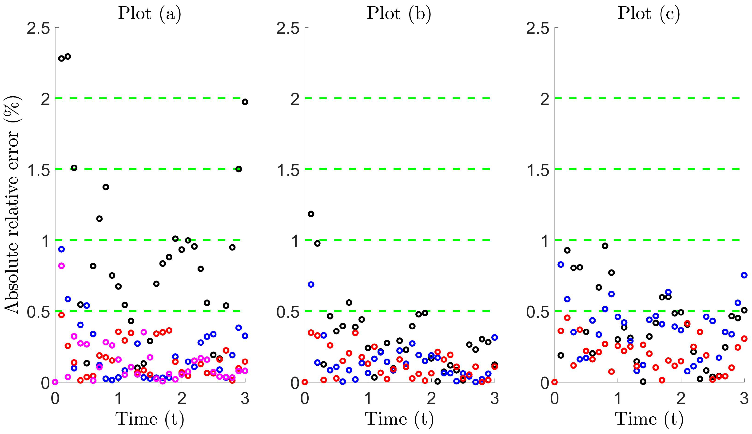
Figure 7 illustrates that a high level of accuracy is maintained, where the error lies roughly within 1% using (i) Model 1 for the Holtsmark case with ${\gamma }_h=0.04$ (magenta circles in Plot (a)) and (ii) Model 2 for all other cases. On comparing the absolute relative error in

Table 4. Tabulated values of the average absolute relative error $\overline{A}$ as defined by (32), to compare the fit between Models 1 (46) and 2 (47) and trap counts. $\overline{A}$ is also included for the anomalous diffusion model; see Figure 3 and Table 2. Boxed values signify ‘equivalence’ between the diffusion and Lévy movement models.

Diffusion	${\mathit{\gamma }}_{\mathit{h}}=0.01$	$0.02$	$0.04$	${\mathit{\gamma }}_{\mathit{c}}=0.0005$	$0.002$	$0.003$	${\mathit{\gamma }}_{\mathit{l}}={10}^{-6}$	$4\times {10}^{-6}$	$2\times {10}^{-5}$
Standard $H=\frac{1}{2}$					2.035
Super $H=\frac{3}{4}$					0.849
Ballistic $H=1$					1.120
Model 1 (46)			0.139
Model 2 (47)	0.162	0.198	0.839	0.123	0.135	0.299	0.194	0.370	0.394

, we find that the proposed diffusion models significantly improve trap count prediction more than what is obtained from super diffusion. Moreover, the numerical values in Table 4 are indicative of equivalence (compare the boxed values to the others), since these values lie within the interval $0<\overline{A}\le 0.5$, also previously seen when comparing standard diffusion to Brownian motion, which are theoretically equivalent movement processes (see Table 1). Evidently, these proposed diffusion models can be used effectively to reproduce trap counts for a system of Lévy walking individuals to a remarkable level of accuracy, yielding almost identical counts.

5. Discussion

The concept of Lévy walks emerging from time-dependent diffusion in the physical or biological sciences in not uncommon. For example, Ott et al. [82] argued that anomalous diffusion of tracer particles in systems of polymer-like breakable micelles (‘living polymers’) provides an experimental realization of a Lévy walk. A more recent example is that of Chen et al. [83], who showed from experiments that active transport within living cells described by time-dependent Brownian walks can self-organize into (truncated) Lévy walks. Other examples demonstrating this concept can be found elsewhere in the literature, e.g., swarming bacteria [84], pollen dispersal [85], etc. Despite this, from an ecological viewpoint, such as insect trapping, the motivation behind time-dependent diffusion, and how this is linked to the type of mechanisms involved, to date, has not been clearly understood [52].

In this study, the diffusion coefficient introduced (43) consists of parameters of ecological significance with obvious meaning, in the sense that they are not all arbitrary and are related to the underlying movement dynamics. One possible explanation of the type of diffusive pattern seen in Figure 6 can be arrived at through the concept of differential energetics [86,87,88]. If an individual executes a large step, then this will incur higher energy costs than a small step, so energy expenditure for different step lengths is a given. In relation to basic individual traits, such as body mass, a heavier body requires a larger force and a larger energy expense to change direction or execute a larger step. Therefore, it may be expected that the frequency of moving long distances is lower for heavier individuals. Furthermore, for those individuals that do prefer to take large steps, this could possibly induce larger rest pauses contributing towards intermittent behavior [89], from which the decrease in the rate of diffusivity can be explained. On the other hand, the mechanisms behind the movement behavior could involve a degree of spatial synchronization of individual variation. In the case of movement with a physiological origin, this could result from a diffusivity distribution as indicated by Petrovskii and Morozov [48] or, alternatively, even time-dependent diffusion. Furthermore, with reference to behavioral effects, a sudden event may trigger a change in behavior in one individual that results in swarming behavior, leading to a change at the population level [90]. It must also be realized that the build up of the insect population and following changes in diffusivity can also be a result of transient environmental factors, e.g., temperature [91], as sudden temperature changes can excite movement or even lead to erratic behavior. If one or more of these factors can bring about diffusive movement varying with time, then as a consequence, the pattern produced by an insect population performing Brownian motion may be indistinguishable from the pattern produced by insects performing Lévy walks. Altogether, it seems that identifying a genuine Lévy walk may be more challenging than previously thought. In light of this, it is not surprising that the Lévy or diffusion controversy has been persistent, with strong evidence arguing for either side; in this study, we have demonstrated that both sides are somewhat equivalent, at least in the context of trapping.

On a final note, we would like to mention some limitations and suggest possible further research directions. Although this study is purely theoretical and attempts to answer some important issues in movement ecology, it is limited to the 1D spatial scale. In a more practical scenario, it would be interesting to see a similar study in a more realistic 2D domain, which would be more relevant to field studies with the trapping of walking/crawling insects [12,28]. The problem would then have enhanced complexity due to the introduction of a single trap of different possible shapes and sizes. For example, Reynolds [92] suggests that trap size will become a relevant quantity when the analysis is extended from the 1D case to higher dimensions. The movement pattern would then be altered, as the effects of trap and field boundaries are realized by enforcing a confined or restricted space [60]. In particular, interest would lie in how the time-dependent diffusion model could be further refined in order to produce trap counts at a high level of accuracy within these different geometries. The diffusion model can then be checked and tested for good agreement against insect trap counts in the real field, given that there is evidence of Lévy-type movement beforehand. Developing a corresponding model in 2D would be the next obvious step to take.

Attempting to model more realistic scenarios would further increase the level of model complexity. For example, in the real field, very rarely, a single trap is installed; rather, a multiple trapping system is implemented [93]. In terms of modeling, the geometry of the domain becomes intrinsically complicated, and the effects of perturbations from each trap may become difficult to unravel. In addition, removing the assumption that the random walk is unbiased would result in directed movement. This can be related to baited traps, which are widely used in practice to increase the frequency of captures [94,95]. Application of a certain agent can induce behavioral responses and attract insects to the trap, such as light, odors or pheromone. Since installation of baited traps considerably alters the insect behavior, they are much more difficult to model [96], and the corresponding theory is largely absent. In this case, the convenient mathematical framework would consist of advection-diffusion equations, where possibly, a time-dependent diffusivity may be used.

6. Concluding Remarks

In this paper, we show that the diffusion coefficients (43) and the reduced version (45) can be incorporated into a time-dependent diffusion model, which can then be used to predict, almost identically, trap counts from a system of individuals who undergo a Lévy walk. Moreover, we show that this can be achieved for a broad range of Lévy tail indices. Furthermore, we find that these proposed diffusion models are much more accurate and effective when compared to super diffusion. Alongside the development of the models, we explore the biological basis for time-dependent diffusion in more detail and interpret parameters in relation to diffusive patterns. We argue that, if these inherently different movement models yield almost identical trap counts, then how important is the movement pattern in the context of trapping? This study suggests that the movement pattern is not that important after all, and rather, emphasis should be on the ecological context, at least in integrated pest monitoring programs.

References

- Burn, A. Integrated Pest Management; Academic Press: New York, NY, USA, 1987. [Google Scholar]
- Kogan, M. Integrated pest management: Historical perspectives and contemporary developments. Annu. Rev. Entomol. 1998, 43, 243–270. [Google Scholar] [CrossRef] [PubMed]
- Millennium Ecosystem Assessment (MEA). Ecosystems and Human Well-Being: Biodiversity Synthesis of the Millennium Ecosystem Assessment; Millennium Ecosystem Assessment World Resources Institute: Washington, DC, USA, 2005. [Google Scholar]
- Cardinale, B.; Duffy, J.; Gonzalez, A.; Hooper, D.; Perrings, C.; Venail, P.; Narwani, A.; Mace, G.; Tilman, D.; Wardle, D.; et al. Biodiversity loss and its impact on humanity. Nature 2012, 486, 59–67. [Google Scholar] [CrossRef] [PubMed]
- Ahmed, D.; van Bodegom, P.; Tukker, A. Evaluation and selection of functional diversity metrics with recommendations for their use in life cycle assessments. Int. J. Life Cycle Assess. 2018. [Google Scholar] [CrossRef]
- Pimentel, D.; Greiner, A. Environmental and socio-economic costs of pesticide use. In Techniques for Reducing Pesticide Use: Economic and Environmental Benefits; Pimentel, D., Ed.; John Wiley and Sons: New York, NY, USA, 1997. [Google Scholar]
- Alavanja, M.; Ross, M.; Bonner, M. Increased cancer burden among pesticide applicators and others due to pesticide exposure. CA Cancer J. Clin. 2013, 62, 120–142. [Google Scholar] [CrossRef] [PubMed]
- Bourguet, D.; Guillemaud, T. Sustainable Agriculture Reviews; The Hidden and External Costs of Pesticide Use; Springer: Berlin, Germany, 2016; Volume 19, pp. 35–120. [Google Scholar]
- Pimentel, D. Amounts of pesticides reaching target pests: Environmental impacts and ethics. J. Agric. Environ. Ethics 1995, 8, 17–29. [Google Scholar] [CrossRef]
- Alyokhin, A.; Baker, M.; Mota-Sanchez, D.; Dively, G.; Grafius, E. Colorado potato beetle resistance to insecticides. Am. J. Potato Res. 2008, 85, 395–413. [Google Scholar] [CrossRef]
- Sohrabi, F.; Shishehbor, P.; Saber, M.; Mosaddegh, M. Lethal and sub-lethal effects of imidacloprid and buprofezin on the sweet potato whitefly parasitoid Eretmocerus mundus (Hymenoptera: Aphelinidae). Crop. Prot. 2013, 45, 98–103. [Google Scholar] [CrossRef]
- Petrovskii, S.; Ahmed, D.; Blackshaw, R. Estimating Insect Population Density. Ecol. Complex 2012, 10, 69–82. [Google Scholar] [CrossRef]
- Holland, J.M.; Perry, J.N.; Winder, L. The within-field spatial and temporal distribution of arthropods in winter wheat. Bull. Entomol. Res. 1999, 89, 499–513. [Google Scholar] [CrossRef]
- Ferguson, A.W.; Klukowski, Z.; Walczak, B.; Perry, J.N.; Mugglestone, M.A.; Clark, S.J.; Williams, I. The spatio-temporal distribution of adult Ceutorhynchus assimilis in a crop of winter oilseed rape in relation to the distribution of their larvae and that of the parasitoid Trichomalus perfectus. Entomol. Exp. Appl. 2000, 95, 161–171. [Google Scholar] [CrossRef]
- Alexander, C.J.; Holland, J.M.; Winder, L.; Woolley, C.; Perry, J.N. Performance of sampling strategies in the presence of known spatial patterns. Ann. Appl. Biol. 2005, 146, 361–370. [Google Scholar] [CrossRef]
- Byers, J.A.; Anderbrant, O.; Lofqvist, J. Effective attraction radius: A method for comparing species attractants and determining densities of flying insects. J. Chem. Ecol. 1989, 15, 749–765. [Google Scholar] [CrossRef] [PubMed]
- Raworth, D.A.; Choi, M. Determining numbers of active carabid beetles per unit area from pitfall-trap data. Entomol. Exp. Appl. 2001, 98, 95–108. [Google Scholar] [CrossRef]
- Turchin, P. Quantitative Analysis of Movement: Measuring and Modelling Population Redistribution in Animals and Plants; Sinauer Associates: Sunderland, MA, USA, 1998. [Google Scholar]
- Okubo, A.; Levin, S. Diffusion and Ecological Problems: Modern Perspectives; Springer: New York, NY, USA, 2001. [Google Scholar]
- Lewis, M.; Maini, P.; Petrovskii, S. Dispersal, Individual Movement and Spatial Ecology; Springer: Berlin, Germany, 2013. [Google Scholar]
- Levin, S.; Cohen, D.; Hastings, A. Dispersal strategies in patchy environments. Theor. Popul. Biol. 1984, 26, 165–180. [Google Scholar] [CrossRef]
- Reichenbach, T.; Mobilia, M.; Frey, E. Mobility promotes and jeopardizes biodiversity in rock-paper-scissors games. Nature 2007, 448, 1046–1049. [Google Scholar] [CrossRef] [PubMed]
- Hengeveld, R. Dynamics of Biological Invasions; Chapman and Hall: London, UK, 1989. [Google Scholar]
- Shigesada, N.; Kawasaki, K. Biological Invasions: Theory and Practice; Oxford University Press: Oxford, UK, 1997. [Google Scholar]
- Petrovskii, S.; Brian, L. Exactly Solvable Models of Biological Invasion; Chapman and Hall/CRC: Boca Raton, FL, USA, 2006. [Google Scholar]
- Petrovskii, S.; Petrovskaya, N.; Bearup, D. Multiscale approach to pest insect monitoring: Random walks, pattern formation, synchronization and networks. Phys. Life Rev. 2014, 11, 467–525. [Google Scholar] [CrossRef] [PubMed]
- Ahmed, D.; Petrovskii, S. Time Dependent Diffusion as a Mean Field Counterpart of Lévy Type Random Walk. Math. Model. Nat. Phenom. 2015, 10, 5–26. [Google Scholar] [CrossRef]
- Bearup, D.; Benefer, C.; Petrovskii, S.; Blackshaw, R. Revisiting Brownian motion as a description of animal movement: A comparison to experimental movement data. Methods Ecol. Evol. 2016, 7, 1525–1537. [Google Scholar] [CrossRef]
- Skellam, J. Random dispersal in theoretical populations. Biometrika 1951, 38, 196–218. [Google Scholar] [CrossRef] [PubMed]
- Kareiva, P.; Shigesada, N. Analyzing insect movement as a correlated random walk. Oecologia 1983, 56, 234–238. [Google Scholar] [CrossRef] [PubMed]
- Kareiva, P. Local movement in herbivorous insecta: Applying a passive diffusion model to mark-recapture field experiments. Oecologia 1983, 57, 322–327. [Google Scholar] [CrossRef] [PubMed]
- Reynolds, A.; Smith, A.; Menzel, R.; Greggers, U.; Reynolds, D.; Riley, J. Displaced honey bees perform optimal scale-free search flights. Ecology 2007, 88, 1955–1961. [Google Scholar] [CrossRef] [PubMed]
- Hapca, S.; Crawford, J.; Young, I. Anomalous diffusion of heterogeneous populations characterized by normal diffusion at the individual level. J. R. Soc. Interface 2009, 6, 111–122. [Google Scholar] [CrossRef] [PubMed]
- Jansen, V.; Mashanova, A.; Petrovskii, S. Model selection and animal movement: “Comment on Lévy walks evolve through interaction between movement and environmental complexity”. Science 2012, 335, 918. [Google Scholar] [CrossRef] [PubMed]
- Ahmed, D. Stochastic and Mean Field Approaches for Trap Count Modelling and Interpretation. Ph.D. Thesis, Leicester University, Leicester, UK, 2015. [Google Scholar]
- Petrovskii, S.; Morozov, A.; Li, B. On a possible origin of the fat-tailed dispersal in population dynamics. Ecol. Complex. 2008, 5, 146–150. [Google Scholar] [CrossRef]
- Mashanova, A.; Olive, T.; Jansen, V. Evidence for intermittency and a truncated power law from highly resolved aphid movement data. J. R. Soc. Interface 2010, 7, 199–208. [Google Scholar] [CrossRef] [PubMed] [Green Version]
- Knell, A.; Codling, E. Classifying area-restricted search (ARS) using a partial sum approach. Theor. Ecol. 2012, 5, 325–329. [Google Scholar] [CrossRef]
- Sims, D.; Southall, E.; Humphries, N.; Hays, G.; Bradshaw, C.; Pitchford, J.; James, A.; Ahmed, M.; Brierley, A.; Hindell, M.; et al. Scaling laws of marine predator search behavior. Nature 2008, 451, 1098–1102. [Google Scholar] [CrossRef] [PubMed]
- Viswanathan, G.; Afanasyev, V.; Buldryrev, S.; Havlin, S.; da Luz, M.R.; Stanley, H. The Physics of Foraging; Cambridge University Press: Cambridge, UK, 2011. [Google Scholar]
- Edwards, A.; Phillips, R.; Watkins, N.; Freeman, M.; Murphy, E.; Afanasyev, V.; Buldyrev, S.; da Luz, M.G.; Raposo, E.; Stanley, H.; et al. Revisiting Lévy flight search patterns of wandering albatrosses, bumblebees and deer. Nature 2007, 449, 1044–1048. [Google Scholar] [CrossRef] [PubMed] [Green Version]
- Benhamou, S. How many animals really do the Lévy walk? Ecology 2007, 88, 1962–1969. [Google Scholar] [CrossRef] [PubMed]
- Shlesinger, M.; Zaslavsky, G.; Klafter, J. Strange kinetics. Nature 1993, 363, 31–37. [Google Scholar] [CrossRef]
- Zaburdaev, Z.; Denisov, S.; Klafter, J. Lévy walks. Rev. Mod. Phys. 2015, 87, 483. [Google Scholar] [CrossRef]
- Viswanathan, G.; Afanasyev, V.; Buldryrev, S.E.A. Lévy flight search patterns of wandering albatrosses. Nature 1996, 381, 413–415. [Google Scholar] [CrossRef]
- Reynolds, A. Olfactory search behavior in the wandering albatross is predicted to give rise to Lévy flight movement patterns. Anim. Behav. 2012, 83, 1225–1229. [Google Scholar] [CrossRef]
- Bartumeus, F.; Catalan, J. Optimal search behavior and classic foraging theory. J. Phys. A 2009, 132, 569–580. [Google Scholar] [CrossRef]
- Petrovskii, S.; Morozov, A. Dispersal in a Statistically Structured Population. Am. Nat. 2008, 173, 278–289. [Google Scholar] [CrossRef] [PubMed]
- Petrovskii, S.; Mashanova, A.; Jansen, V. Variation in individual walking behavior creates the impression of a Lévy flight. Proc. Natl. Acad. Sci. USA 2011, 108, 8704–8707. [Google Scholar] [CrossRef] [PubMed]
- Auger-Méthé, M.; Derocher, A.; Plank, M.; Codling, E.; Lewis, M. Differentiating the Lévy walk from a composite correlated random walk. Methods Ecol. Evol. 2015, 6, 1179–1189. [Google Scholar] [CrossRef]
- De Jager, M.; Weissing, F.; Herman, P.; Nolet, B.; vande Koppel, J. Response to Comment on “Lévy walks evolve through interaction between movement and environmental complexity”. Science 2012, 335, 918. [Google Scholar] [CrossRef]
- Codling, E. Pest insect movement and dispersal as an example of applied movement ecology. Comment on “Multiscale approach to pest insect monitoring: Random walks, pattern formation, synchronization, and networks” by Petrovskii, Petrovskaya and Bearup. Phys. Life Rev. 2014, 11, 533–535. [Google Scholar] [CrossRef] [PubMed]
- Petrovskii, S.; Petrovskaya, N.; Bearup, D. Multiscale ecology of agroecosystems is an emerging research field that can provide a stronger theoretical background for the integrated pest management. Reply to comments on “Multiscale approach to pest insect monitoring: Random walks, pattern formation, synchronization, and networks”. Phys. Life Rev. 2014, 11, 536–539. [Google Scholar] [PubMed]
- Grimm, V.; Railsback, S. Individual Based Modelling and Ecology; Princeton University Press: Princeton, NJ, USA, 2005. [Google Scholar]
- Petrovskii, S.; Petrovskaya, N. Computational ecology as an emerging science. Interface Focus 2012, 2, 241–254. [Google Scholar] [CrossRef] [PubMed]
- Bearup, D.; Petrovskaya, N.; Petrovskii, S. Some analytical and numerical approaches to understanding trap counts resulting from pest insect immigration. Math. Biosci. 2015, 263, 143–160. [Google Scholar] [CrossRef] [PubMed]
- Pyke, G. Understanding movements of organisms: It’s time to abandon the Lévy foraging hypothesis. Methods Ecol. Evol. 2015, 6, 1–16. [Google Scholar] [CrossRef]
- Weiss, G. Aspects and Applications of the Random Walk; North Holland Press: Amsterdam, The Netherlands, 1994. [Google Scholar]
- Codling, E.; Plank, M.; Benhamou, S. Random walk models in biology. J. R. Soc. Interface 2008, 5, 813–834. [Google Scholar] [CrossRef] [PubMed]
- Bearup, D.; Petrovskii, S. On time scale invariance of random walks in confined space. J. Theor. Biol. 2015, 367, 230–245. [Google Scholar] [CrossRef] [PubMed]
- Viswanathan, G.; Buldyrev, S.; Havlin, S. Optimizing the success of random searches. Nature 1999, 401, 911–914. [Google Scholar] [CrossRef] [PubMed]
- Knighton, J.; Dapkey, T.; Cruz, J. Random walk modeling of adult Leuctra ferruginea (stonefly) dispersal. Ecol. Inf. 2014, 19, 1–9. [Google Scholar] [CrossRef]
- Nathan, R.; Getz, W.; Revilla, E.; Holyoak, M.; Kadmon, R.; Saltz, D.; Smouse, P. A movement ecology paradigm for unifying organismal movement research. Proc. Natl. Acad. Sci. USA 2008, 105, 19052–19059. [Google Scholar] [CrossRef] [PubMed]
- Benhamou, S. Of scales and stationarity in animal movements. Ecol. Lett. 2014, 17, 261–272. [Google Scholar] [CrossRef] [PubMed]
- Murray, J. Mathematical Biology: I. An Introduction, 3rd ed.; Springer: Berlin, Germany, 2002. [Google Scholar]
- Crank, J. The Mathematics of Diffusion, 2nd ed.; Oxford University Press: Oxford, UK, 1975. [Google Scholar]
- Einstein, A. Über die von der molekularkinetischen Theorie der Wärme geforderte Bewegung von in ruhenden Flüssigkeiten suspendierten Teilchen. Ann. Phys. 1905, 17, 549–560. [Google Scholar] [CrossRef]
- Sornette, D. Critical Phenomena in Natural Sciences, 2nd ed.; Springer: Berlin, Germay, 2004. [Google Scholar]
- Balescu, R. Equilibrium and Non-Equilibrium Statistical Mechanics; John Wiley: New York, NY, USA, 1975. [Google Scholar]
- Kölzsch, A.; Alzate, A.; Bartumeus, F.; de Jager, M.; Weerman, E.; Hengeveld, G.; Naguib, M.; Nolet, B.; van de Koppel, J. Experimental evidence for inherent Lévy search behavior in foraging animals. Proc. R. Soc. B 2015, 282. [Google Scholar] [CrossRef] [PubMed]
- Nolan, J. Stable Distributions—Models for Heavy Tailed Data; Birkhauser: Boston, MA, USA, 2015; In Progress: Chapter 1; Available online: academic2.american.edu/~jpnolan (accessed on 1 December 2017).
- Chambers, J.; Mallows, C.; Stuck, B. A method for simulating stable random variables. JASA 1976, 71, 340–344. [Google Scholar] [CrossRef]
- Weron, R. On the Chambers-Mallows-Stuck method for simulating skewed stable random variables. Stat. Probabil. Lett. 1996, 28, 165–171, See also Weron, R. Correction to: On the Chambers-Mallows-Stuck Method for Simulating Skewed Stable Random Variables, Research Report HSC/96/1, Wroc Law University of Technology, 1996. Available online: http://www.im.pwr.wroc.pl/~hugo/Publications.html (accessed on 1 December 2017). [CrossRef] [Green Version]
- Zolotarev, V. One-Dimensional Stable Distributions; American Mathematical Society: Providence, RI, USA, 1986. [Google Scholar]
- Samorodnitsky, G.; Taqqu, M. Stable Non-Gaussian Random Processes; Chapman and Hall: Boca Raton, FL, USA, 1994. [Google Scholar]
- Holmes, E.E. Are diffusion models too simple? A comparison with telegraph models of invasion. Am. Nat. 1993, 142, 779–795. [Google Scholar] [CrossRef] [PubMed]
- Brose, U. Body-mass constraints on foraging behavior determine population and food-web dynamics. Funct. Ecol. 2010, 24, 28–34. [Google Scholar] [CrossRef]
- Klafter, J.; Sokolov, I. Anomalous diffusion spreads its wings. Phys. World 2005, 18, 29–32. [Google Scholar] [CrossRef]
- Malchow, H.; Petrovskii, S.; Venturino, E. Spatiotemporal Patterns in Ecology and Epidemiology: Theory, Models, and Simulations; Chapman and Hall/CRC: Boca Raton, FL, USA, 2008. [Google Scholar]
- Rosenzweig, M.; MacArthur, R. Graphical representation and stability conditions of predator-prey interaction. Am. Nat. 1963, 97, 209–223. [Google Scholar] [CrossRef]
- Choules, J.; Petrovskii, S. Which Random Walk is Faster? Methods to Compare Different Step Length Distributions in Individual Animal Movement. Math. Model. Nat. Phenom. 2017, 12, 22–45. [Google Scholar] [CrossRef]
- Ott, A.; Bouchaud, J.; Langevin, D.; Urbach, W. Anomalous diffusion in ‘‘living polymers’’: A genuine Lévy flight? Phys. Rev. Lett. 1990, 65, 2201–2204. [Google Scholar] [CrossRef] [PubMed]
- Chen, K.; Wang, B.; Granick, S. Memoryless self-reinforcing directionality in endosomal active transport within living cells. Nat. Mater. 2015, 14, 589–593. [Google Scholar] [CrossRef] [PubMed]
- Ariel, G.; Rabani, A.; Benisty, S.; Partridge, J.; Harshey, R.; Be’er, A. Swarming bacteria migrate by Lévy Walk. Nat. Commun. 2015, 6, 8396. [Google Scholar] [CrossRef] [PubMed]
- Vallaeys, V.; Tyson, R.; Lane, W.; Deleersnijder, E.; Hanert, E. A Lévy-flight diffusion model to predict transgenic pollen dispersal. J. R. Soc. Interface 2017, 14. [Google Scholar] [CrossRef] [PubMed]
- Harold, H. Energetics of Desert Invertebrates; Springer: Berlin, Germany, 1996. [Google Scholar]
- El Baidouri, F.; Venditti, C.; Humphries, S. Independent evolution of shape and motility allows evolutionary flexibility in Firmicutes bacteria. Nat. Ecol. Evol. 2016, 9, 0009. [Google Scholar] [CrossRef] [PubMed]
- Halsey, L. Terrestrial movement energetics: Current knowledge and its application to the optimising animal. J. Exp. Biol. 2016, 219, 1424–1431. [Google Scholar] [CrossRef] [PubMed]
- Kramer, D.; McLaughlin, R. The Behavioral Ecology of Intermittent Locomotion. Am. Zool. 2015, 41, 137–153. [Google Scholar] [CrossRef]
- Jervis, M. Insects as Natural Enemies: A Practical Perspective; Springer: Berlin, Germany, 2005; p. 281. [Google Scholar]
- Tyson, R. Pest control: A modeling approach. Comment on “Multiscale approach to pest insect monitoring: Random walks, pattern formation, synchronization, and networks” by S. Petrovskii, N. Petrovskaya, D. Bearup. Phys. Life Rev. 2014, 11, 526–528. [Google Scholar] [CrossRef] [PubMed]
- Reynolds, A. Extending Lévy search theory from one to higher dimensions: Lévy walking favours the blind. Proc. Math. Phys. Eng. Sci. 2015, 471. [Google Scholar] [CrossRef] [PubMed]
- Brennan, K.; Majer, J.; Reygaert, N. Determination of an Optimal Pitfall Trap Size for Sampling Spiders in a Western Australian Jarrah Forest. J. Insect Conserv. 1999, 3, 297–307. [Google Scholar] [CrossRef]
- Elkinton, J.; Lance, D.; Boettner, G.; Khrimian, A.; Leva, N. Evaluation of pheromone-baited traps for winter moth and Bruce spanworm (Lepidoptera: Geometridae). J. Econ. Entomol. 2011, 104, 494–500. [Google Scholar] [CrossRef] [PubMed]
- Tuf, I.; Chmelík, V.; Dobroruka, I.; Hábová, L.; Hudcová, P.; Ŝipoŝ, J.; Staŝiov, S. Hay-bait traps are a useful tool for sampling of soil dwelling millipedes and centipedes. Zookeys 2015, 510, 197–207. [Google Scholar] [CrossRef] [PubMed]
- Yamanaka, T.; Tatsuki, S.; Shimada, M. An individual-based model for sex-pheromone-oriented flight patterns of male moths in a local area. Ecol. Model. 2003, 161, 35–51. [Google Scholar] [CrossRef]
- Morton, K.; Mayers, D. Numerical Solution of Partial Differential Equations: An Introduction; Cambridge University Press: Cambridge, UK, 1994. [Google Scholar]
- Holmes, M. Introduction to Numerical Methods in Differential Equations; Springer: Berlin, Germany, 2006. [Google Scholar]
- Strauss, W. Partial Differential Equations: An Introduction; John Wiley and Sons: Hoboken, NJ, USA, 2008. [Google Scholar]