Role of Bi-Directional Migration in Two Similar Types of Ecosystems


1
Department of Mathematics, Visva-Bharati University, Santiniketan 731235, India
2
Department of Mathematics, Faculty of Science & Arts-Rabigh, King Abdulaziz University, Rabigh 25732, Saudi Arabia
3
Department of Mathematics, University of Florida, Gainesville, FL 32611, USA
4
Agricultural and Ecological Research Unit, Indian Statistical Institute 203, B. T. Road, Kolkata 700108, India
*
Author to whom correspondence should be addressed.
†
Work supported by NSF grant DMS-1515661.
Mathematics 2018, 6(3), 36; https://doi.org/10.3390/math6030036
Submission received: 15 January 2018
/
Revised: 18 February 2018
/
Accepted: 20 February 2018
/
Published: 2 March 2018
(This article belongs to the Special Issue Progress in Mathematical Ecology)
Abstract
:Migration is a key ecological process that enables connections between spatially separated populations. Previous studies have indicated that migration can stabilize chaotic ecosystems. However, the role of migration for two similar types of ecosystems, one chaotic and the other stable, has not yet been studied properly. In the present paper, we investigate the stability of ecological systems that are spatially separated but connected through migration. We consider two similar types of ecosystems that are coupled through migration, where one system shows chaotic dynamics, and other shows stable dynamics. We also note that the direction of the migration is bi-directional and is regulated by the population densities. We propose and analyze the coupled system. We also apply our proposed scheme to three different models. Our results suggest that bi-directional migration makes the coupled system more regular. We have performed numerical simulations to illustrate the dynamics of the coupled systems.
1. Introduction
In mathematical biology, population theory plays an important role. Historically, the first model of population dynamics was formulated by Malthus [1] and was later on adapted for more realistic situations by Verhulst [2]. Lotka and Volterra [3,4] first modeled oscillations occurring in natural populations. Subsequently, the Lotka–Volterra model was modified by several researchers, and many of them observed chaotic dynamics [5,6,7,8,9]. The occurrence of chaos in a simple ecological system motivated researchers to investigate complex dynamical behaviors of ecological systems, such as bi-stability, bifurcation and chaos. However, in real-world populations, the evidence of chaos is rare. In ecology, until now, many researchers have investigated three-species food chain/web models with the aim of controlling the chaos by incorporating several biological phenomena [10,11,12].
Spatial structure is an important factor in ecological systems. Natural systems are rarely isolated but rather interact among themselves as well as with their natural surroundings, and the dynamics of ecological systems connected by migration are very different from the dynamics of the individual systems. The concept of a metapopulation is a formalism to describe spatially separated interacting populations [13,14]. A metapopulation consists of a group of spatially separated populations living in patches; individuals are allowed to migrate to surrounding patches. Levins (1969) [13] proposed a metapopulation theory and applied it in a pest-control situation. In landscape ecology and conservation biology, the idea of a metapopulation plays an important role [15,16].
In population biology, two systems can be coupled through migration, which is a common biological phenomenon and plays a vital role in the stability of ecosystems. Migration has been studied in a variety of taxa [17,18,19]. In the stability of an ecosystem, migration can have a stabilizing effect [20,21,22,23]. Holt (1985) [23] observed that passive dispersal between sink and source habitats can stabilize an otherwise unstable system. MacCullum observed that immigration could stabilize a chaotic system of the crown of thorns starfish Acanthaster planci and its associated larval recruitment patterns [21]. Stone and Hart [22] observed that a discrete-time chaotic system could be stabilized by constant immigration. Silva et al. [24] also synchronized chaotic oscillations of uncoupled populations through migration. Furthermore, it has been established that unstable equilibria of a single-patch predator–prey model cannot be stabilized by coupling with identical patches [25]. The persistence of coupled locally unstable systems depends on asynchronous behaviors between the populations [25,26,27]. Ruxton [28] showed that weak coupling between two chaotic systems exhibited simple cycles or remained at a stable level and reduced populations’ extinction probabilities. Recently, Pal et al. [29] investigated the effect of bi-directional migration on the stability of two non-identical ecosystems, which were connected through migration. They observed that an increase in the rate of migration could stabilize the non-identical coupled ecosystem. The above observations clearly indicate that migration has a major role in stabilizing chaotic ecosystems. However, the role of bi-directional migration for two similar types of ecosystems, where one is chaotic and the other is stable in nature, has not yet been investigated properly.
In the present paper, we consider metapopulation dynamics of spatially separated food webs that are connected through bi-directional migrations. Our aim of the present study is to investigate the role of migration on the stability of a coupled ecosystem for which one system shows chaotic dynamics, and the other system shows stable dynamics. In the next section, we formulate the model and analyze its behavior regarding the interior equilibrium point. In Section 3, we show the applications of the present scheme in three different models. Finally, the paper ends with a brief conclusion.
2. General Model Formulation and Stability Analysis
Two isolated systems can be coupled via migration. We consider the general case of two coupled ecological systems:
where X and Y are the variables in the vector notation. The individual systems are described by the functions and ; and are coupling functions. The equilibrium solutions of the uncoupled system are given by and . When coupling occurs, the equilibrium points of the system given by Equation (1) are given by .
Now we consider two three-species food-chain ecological systems that are coupled through bi-directional migrations. In bi-directional migration, a population can migrate from one patch to another depending on the population densities. The flow of the migration is from higher to lower density. Therefore, in bi-directional migration, the migration depends on the relative density difference between two patches. Then Equation (1) with bi-directional migration can be written as
where are the populations of system 1 and are the populations of system 2; and are the functions describing systems 1 and 2, respectively; are the migration coefficients of the three different populations. To study the stability behavior of the coupled system around the interior equilibrium point , we have to calculate the Jacobian matrix of the system given by Equation (2) at the interior equilibrium point. The Jacobian matrix at is
where the
- , , , , , , , ,
- , , , , , , ,
- , , and
suffixes denote the partial derivatives with respect to the corresponding variable.
The characteristic equation of the above Jacobian matrix is
where
- with , ,
- ,
- , ,
- and .
Now, the eigenvalues of the characteristic equation are negative or have negative real parts if all Routh–Hurwitz (RH) determinants () are positive, where , and , where if .
3. Applications
Migration within a population with spatial subdivision is important in some species and systems. It is observed that, if two identical patches are coupled through migration, then the coupled system acts exactly as a single-patch system. The persistence of coupled locally unstable systems depends on asynchrony behaviors among populations [25,26,27]. It is to be noted that two identical chaotic systems cannot be stabilized by diffusive migration. Here we consider two tri-trophic food-chain systems of the same type with different parameter values, where one system shows chaotic dynamics and the other system shows stable dynamics. We also note that the two tri-trophic food web systems are spatially separated but are connected through bi-directional migrations. In this section, we describe the application of the above scheme developed in Section 2 to three different models, namely, the Hastings–Powell (HP) model, the Upadhyay–Rai (UR) model and the Priyadarshi–Gakkhar (PG) model, which are able to produce stable dynamics as well as chaotic dynamics for different sets of parameter values.
3.1. Hastings–Powell Model
In 1991, Hastings and Powell [6] proposed and analyzed a three-species food-chain model with a Holling type II functional response. The model is known for exhibiting chaotic dynamics in a continuous-time food-chain model. The non-dimensional HP model is governed by the following equations:
where x, y and z are the densities of the prey, middle-predator and top-predator populations, respectively; and are the non-negative parameters that have the usual meanings [6]. Hastings and Powell [6] studied the model given by Equation (3) and observed switching of the dynamics of the system between stable focus, limit cycle oscillations and chaos by changing the parameter .
Coupling between Chaotic HP Model and Stable HP Model
The HP model shows different dynamical behaviors, including chaos. In the present section, we investigate the dynamics of the coupled ecosystem, for which one HP system shows chaotic dynamics and the other HP system shows stable dynamics. Here, we assume that the two different systems are connected by migration and that the direction of the migration is bi-directional. Further, all populations are free to migrate from one system to another. We denote the chaotic HP system with subscript 1 and the stable HP system with subscript 2. The coupled system is governed by the following equations:
where are the migration coefficients of the prey, middle-predator and top-predator populations, respectively. We assume that two systems differ only in the parameter in Equation (3); and are the parameters corresponding to systems 1 and 2, respectively.
Non-Negativity of the Solutions: We let be the non-negative octant in . Then the interaction functions of the system given by Equation (4) are continuously differentiable and locally satisfy Lipschitz conditions in . Thus, any solution of the system given by Equation (4) with non-negative initial conditions satisfies the non-negativity condition and exists uniquely in the interval for some ([30], Theorem A.4).
Boundedness of the Solutions:
We define a function
Applying the theorem of differential inequality [31], we obtain which implies that for all . Therefore, all the solutions of the system given by Equation (4) are bounded.
Hence, all the solutions of the system given by Equation (4), which are initiated in , are positively invariant in the region .
Now we describe the numerical simulations for the system given by Equation (3) and the coupled system given by Equation (4) by considering the following parameter values:
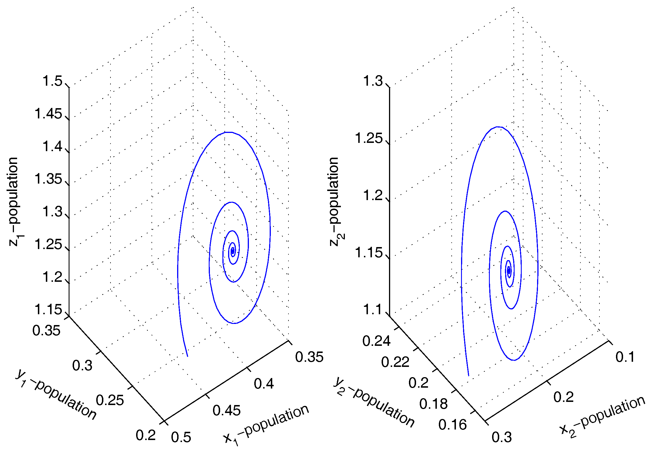
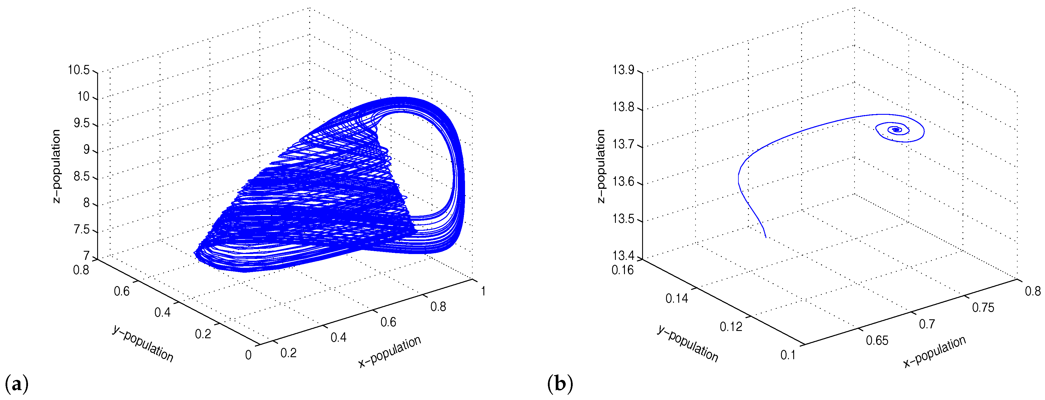
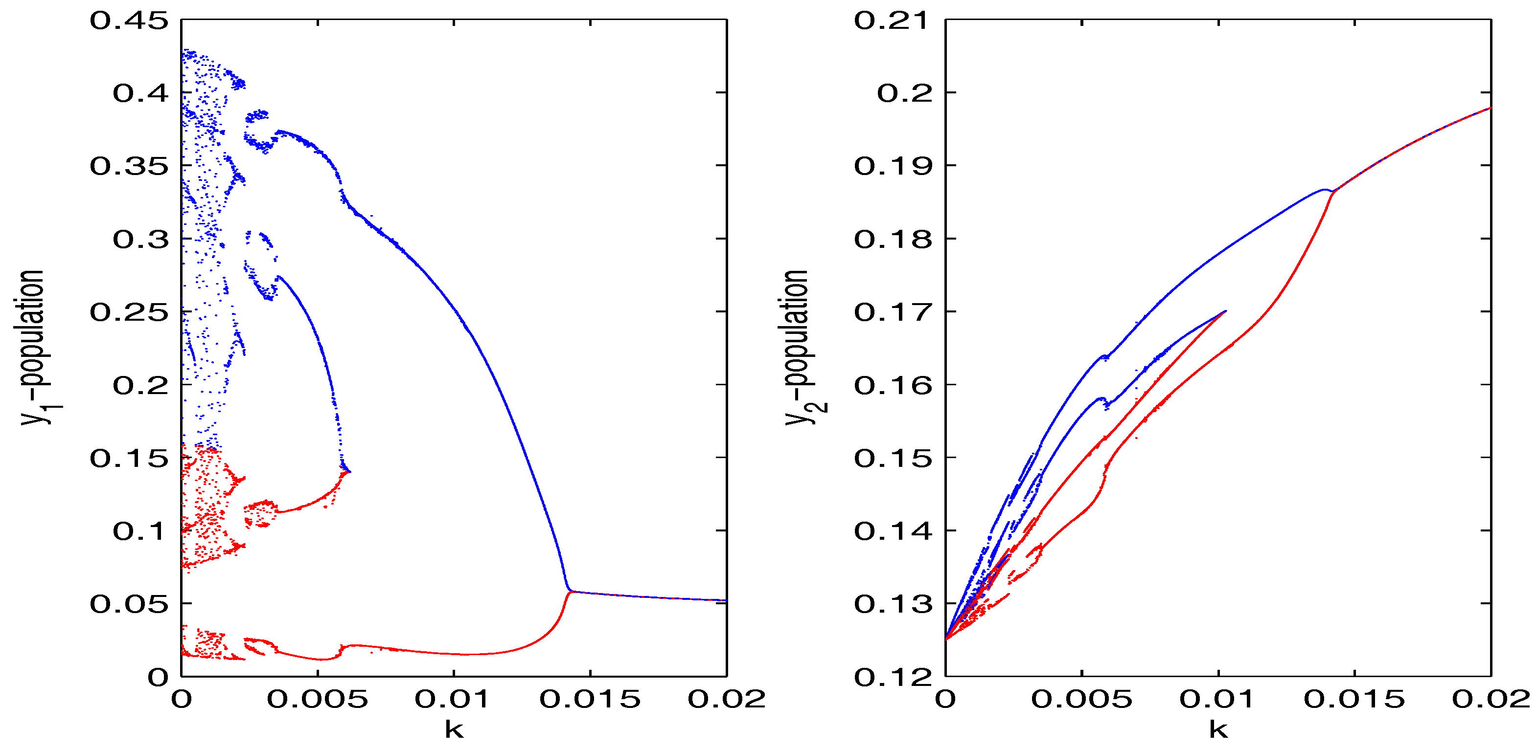
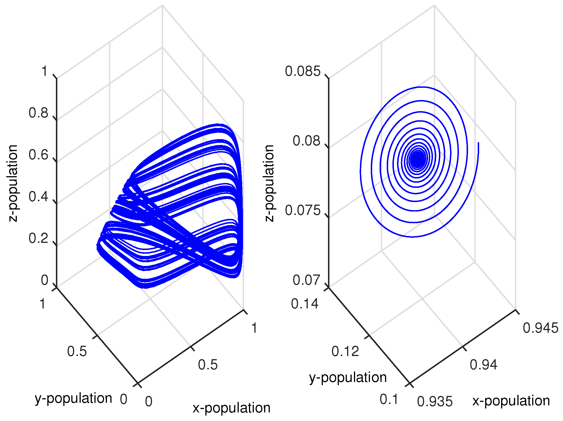
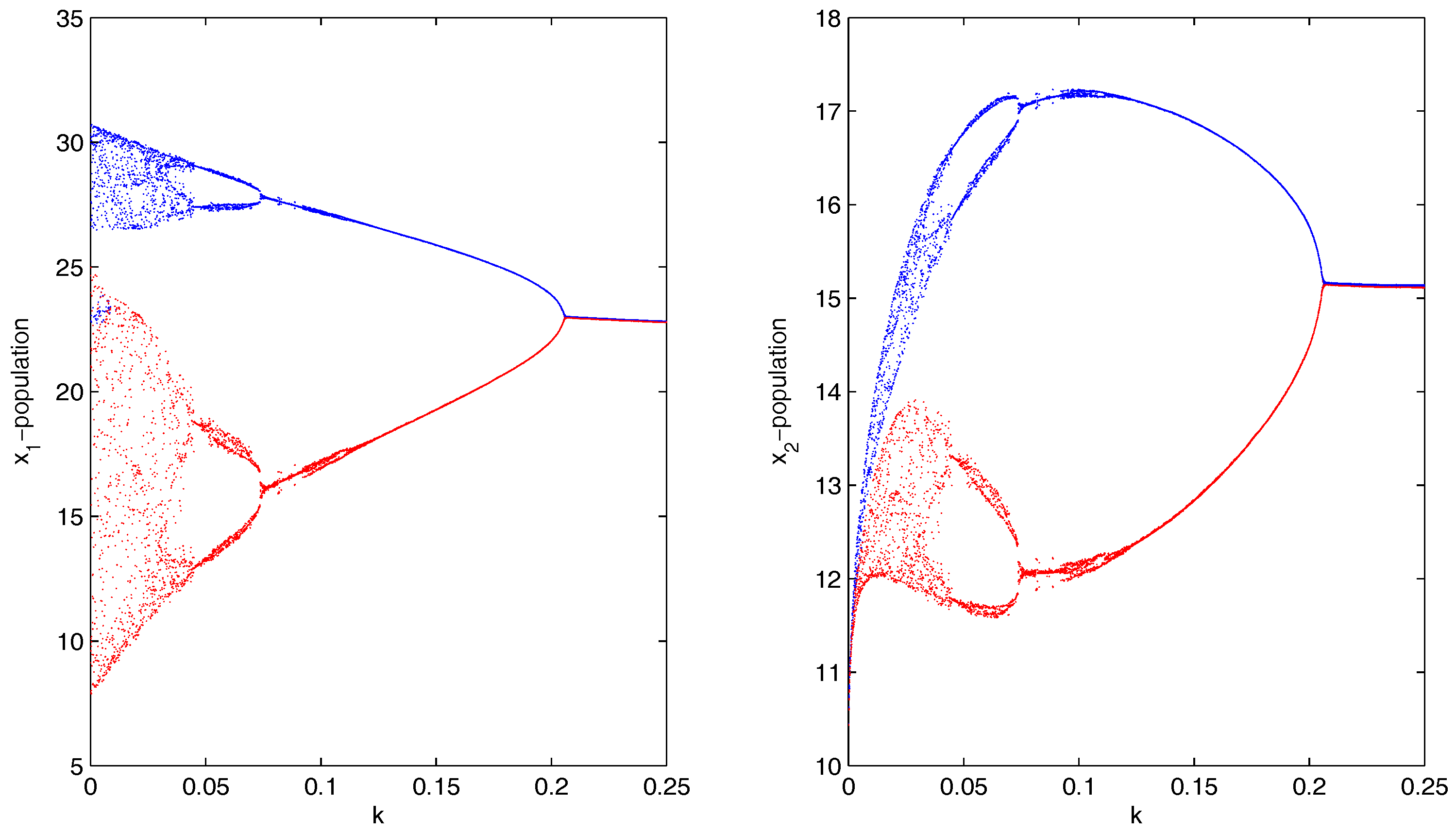
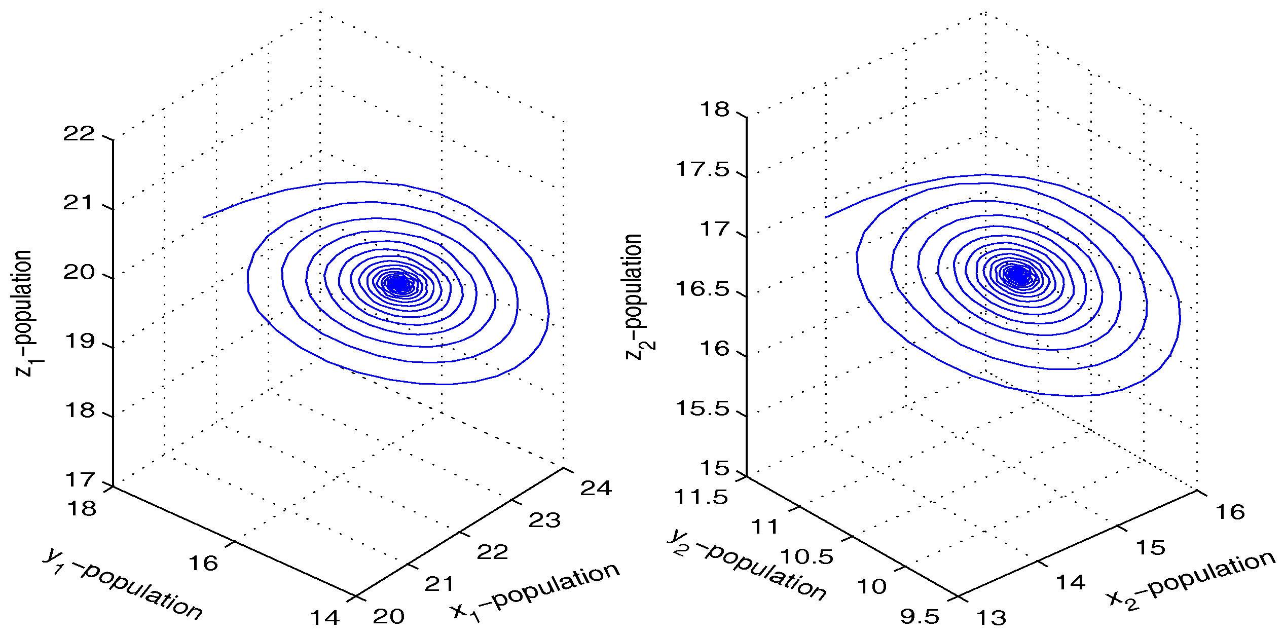
which were taken from [6]. Choosing , then the coupled system given by Equation (4) remained chaotic for any coupling strength (migration rate). We then chose two different values of and , and the HP model of Equation (3) showed chaotic dynamics and stable dynamics. For system 1, we set , so that the system showed chaotic dynamics, and for system 2, we set , so that the system showed stable dynamics (Figure 1). The initial condition for the simulation of the coupled system given by Equation (4) was . We could then investigate the effect of bi-directional migration between the two systems. For simplicity, we considered and drew the bifurcation diagram of the coupled system of Equation (4) with respect to the rate of migration k (Figure 2). It is to be noted that in the absence of migration (), system 1 showed chaotic dynamics and system 2 showed stable dynamics. When we introduced migration between these two systems, then the coupled system became stable through a Hopf bifurcation when the migration rate (k) crossed a threshold value, (Figure 2). We observed that a small migration destabilized the stable system, and the coupled system showed higher periodic and chaotic oscillations, but if the strength of migration was increased gradually, then the coupled system became stable. We also observed that for , the coupled system of Equation (4) had a unique positive interior equilibrium . We also obtained the RH determinants, , , , , , and , which satisfied the RH stability criterion of order 6. The eigenvalues of the coupled system given by Equation (4) were . Hence, the system given by Equation (4) was stable around the positive interior equilibrium (Figure 3).
Further, we performed numerical simulations of the coupled system for the realistic parameter values considered by McCann and Yodzis [32]. McCann and Yodzis [32] considered the modified HP model [6]; they produced a range of more “plausible” parameter values and demonstrated the existence of chaos for a wide range of these values. We considered the following parameter values:
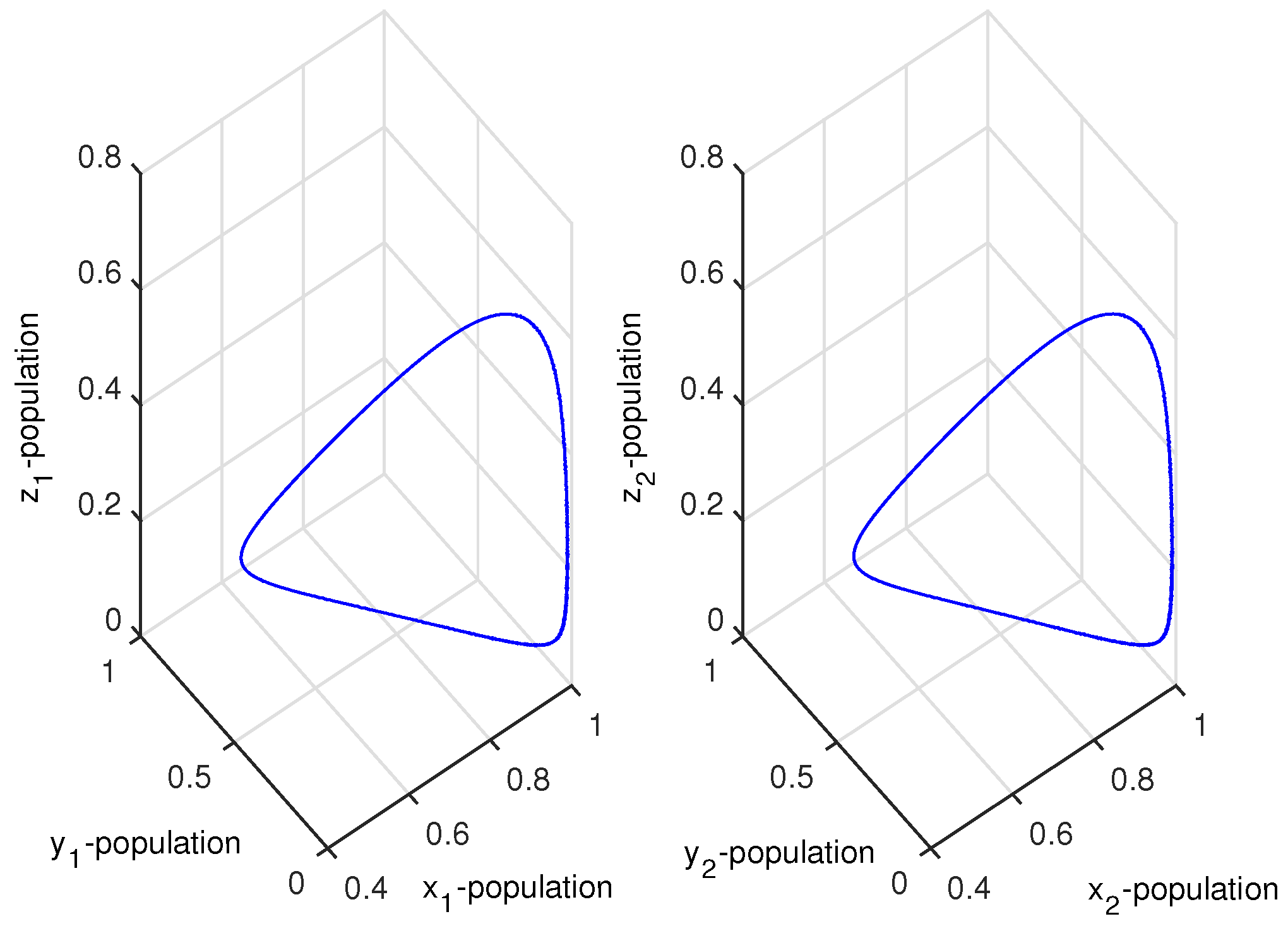
which were taken from [32]. The model and the meaning of the parameter values are given in [32]. For system 1, we set , so that the system showed chaotic dynamics, and for system 2, we set , so that the system showed stable dynamics (Figure 4). The initial condition for the simulations of the coupled system was . If we introduced migration between the two systems (chaotic system and stable system), then the coupled system showed limit cycle oscillations via period-halving bifurcations (Figure 5). We observed that a gradual increase in migration made the coupled system switch its stability from chaotic dynamics to limit cycle oscillations (Figure 6). Therefore, migration could stabilize the coupled system by producing stable focus or more regular oscillations.
3.2. Upadhyay–Rai Model
Upadhyay and Rai [7,33] proposed and analyzed a tri-trophic food-chain model by considering the middle predator as a specialist predator and the top predator as a generalist predator.
The prey–specialist predator–generalist system is governed by the following equations [7,33]:
where x, y and z are the densities of the prey, specialist predator, and generalist predator populations, respectively; and c are the non-negative parameters that have the usual meanings [7,33]. In the above model, the prey population (x) grows logistically; the specialist predator (y) predates prey (only food item available to the specialist predator) via a Holling type II functional response; the generalist predator (z) sexually reproduces, its population growing quadratically () and decaying as a result of intraspecific competition (). Additionally, males and females in the generalist predator population are assumed to be equal in terms of numbers, and the mating frequency is directly proportional to the number of males as well as the number of females. The interaction between the generalist predator and specialist predator follows a modified Leslie–Gower scheme. Here, the specialist middle predator is the favourite food choice of the generalist top predator and the generalist predator feeds on other food items (alternative food resources), in case of a short supply of the middle predator.
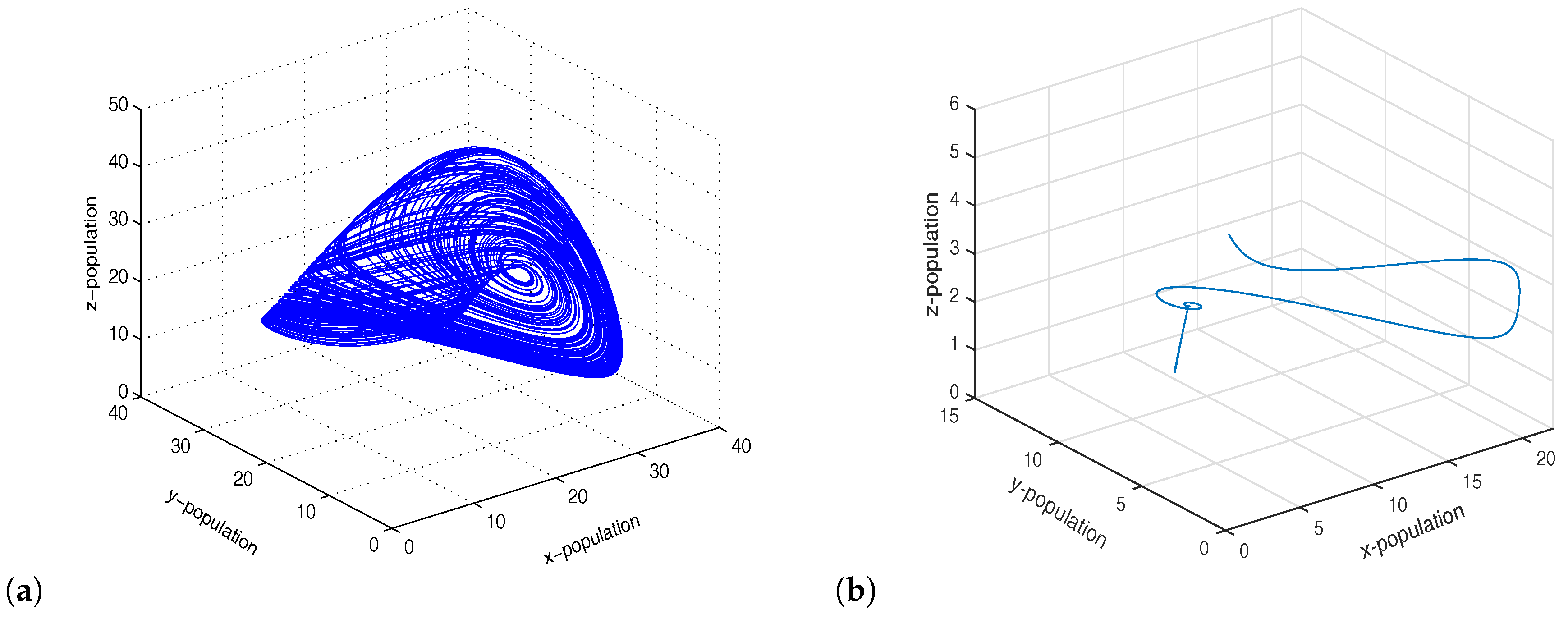
It is to be noted here that the system given by Equation (8) is not always dissipative, and the solutions may blow-up in finite time (explosive instability) depending on the parameter values and initial conditions [34]. In recent literature, few researchers have investigated different models that show finite-time blow-up in the solutions [34,35,36,37,38,39,40]. However, the above system given by Equation (8) shows very rich dynamics when . Upadhyay and Rai [7,33] explored chaotic dynamics in the system by increasing the intrinsic growth rate .
Coupling between Chaotic UR Model and Stable UR Model
In this section, we denote the chaotic UR system with the subscript 1 and the stable UR system with the subscript 2. The coupled system is governed by the following equations:
where are the migration coefficients of the prey, specialist predator and generalist predator populations, respectively. We assume that two systems differ only in the parameter in Equation (8); and are the parameters corresponding to systems 1 and 2, respectively.
Now we describe the numerical simulations of the system given by Equation (8) and the coupled system given by Equation (9). The set of parameters were as follows:
which were taken from [33]. Choosing , then the coupled system given by Equation (8) remained chaotic for any coupling strength (migration rate). We then chose two different values of and , and the UR model given by Equation (8) showed chaotic dynamics and stable dynamics, respectively (Figure 7). For system 1, we set , so that the system showed chaotic dynamics, and for system 2, we set , so that the system showed stable dynamics. The initial condition for the simulations of the coupled system given by Equation (9) was . We then investigated the effect of bi-directional migration on the two systems. For simplicity, we considered and drew the bifurcation diagram of the coupled system given by Equation (9) with respect to the rate of migration k (Figure 8). We observed that the coupled system given by Equation (9) became stable through a Hopf bifurcation when the migration coefficient crossed a threshold value . We observed that when the migration was weak (k small), the stable system became unstable and the coupled system showed higher periodic and chaotic oscillations, but if the strength of migration was increased gradually, then the coupled system became stable. Further, we observed that for , the coupled system given by Equation (9) had a unique positive interior equilibrium . We also obtained the RH determinants , , , , , and , which satisfied the RH stability criterion of order 6. The eigenvalues of the coupled system given by Equation (9) were . Hence, the coupled system given by Equation (9) was stable around the positive interior equilibrium (Figure 9).
3.3. Priyadarshi–Gakkhar Model
Priyadarshi and Gakkhar [9] proposed and analyzed a tri-trophic food-web model consisting of a Leslie–Gower-type generalist predator, where the middle predator is a specialist predator and the top predator is a generalist predator.
The prey–specialist predator–generalist predator system is governed by the following equations [9]:
where x, y and z are the densities of the prey, specialist predator, and generalist predator populations, respectively. The parameters and are non-negative parameters that have the usual meanings [9]. The formulation of the above model is similar to that of the UR model. However, in the above model, the specialist predator predates prey according to a Holling type II functional response, whereas the generalist predator predates prey and the specialist predator following a modified Holling type II functional response. It is to be noted that the system given by Equation (11) may not be dissipative and shows the blow-up phenomenon depending on the parameter values and initial conditions [34]. Priyadarshi and Gakkhar [9] explored a “snail-shell” chaotic attractor in the system.
Coupling between Chaotic PG Model and Stable PG Model
In this section, we investigate the dynamics of the coupled ecosystem, where one PG system shows chaotic dynamics and the other PG system shows stable dynamics. Here, we consider that two different systems are connected by bi-directional migration. We assume that all populations are free to migrate from one system to the other. We denote the chaotic PG system with the subscript 1 and the stable PG system with the subscript 2. The coupled system is governed by the following equations:
where are the migration coefficients of the prey, specialist predator and generalist predator populations, respectively. We assume that two systems differ only in the parameter in Equation (11); , are the parameters corresponding to systems 1 and 2, respectively.
In numerical simulations, we considered the following parameter values:
which were taken from [9]. Choosing , then the coupled system given by Equation (11) remained chaotic for any coupling strength (migration rate). Choosing two different values of and , then the PG model of Equation (11) showed chaotic dynamics and stable dynamics (Figure 10). For system 1, we set , so that the system showed chaotic dynamics, and for system 2, we set , so that the system showed stable dynamics. The initial condition for the simulation of the coupled system given by Equation (12) was . We then investigated the effect of bi-directional migration on the two systems. For simplicity, we considered and drew the bifurcation diagram of the coupled system given by Equation (12) with respect to the rate of migration k (Figure 11). We observed that the coupled system became stable through a Hopf bifurcation when the migration rate (k) crossed a threshold value, (Figure 11). We observed that weak migration destabilized the stable system, but if the strength of the migration was increased gradually, then the coupled system became stable. Further, we observed that for , the coupled system given by Equation (12) had a unique positive interior equilibrium . We also obtained the RH determinants , , , , , and , which satisfied the RH stability criterion of order 6. The eigenvalues of the coupled system given by Equation (12) were . Hence, the system given by Equation (12) was stable around the positive interior equilibrium (Figure 12).
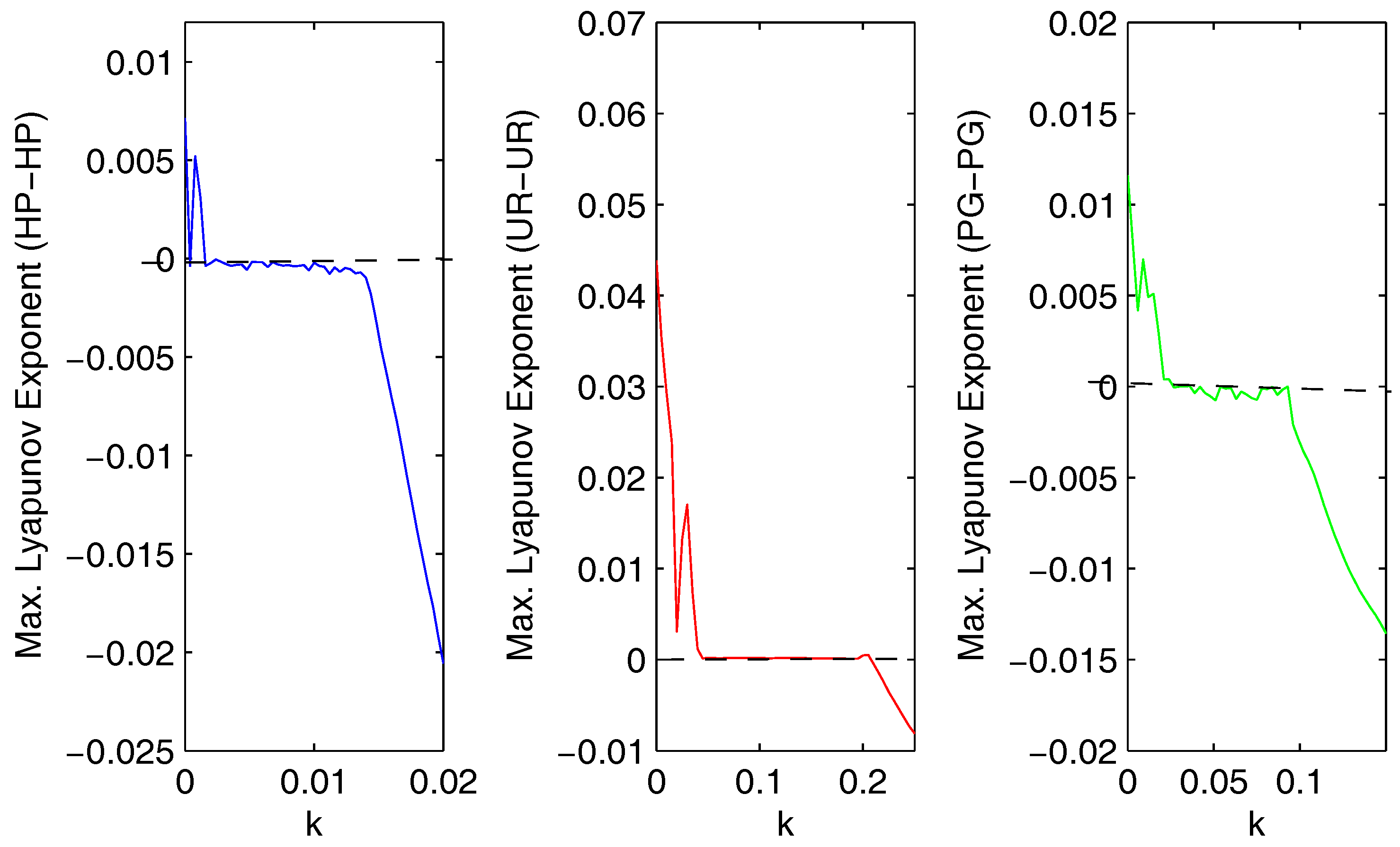
We calculated the maximum Lyapunov exponent (Figure 13) for the coupled systems given by Equations (4), (9) and (12) with respect to the coupling strength (k). We observed that if we increased the strength of migration, then the value of the maximum Lyapunov exponent became negative. The maximum Lyapunov exponent (Figure 13) confirmed that the coupled systems (HP–HP, UR–UR, and PG–PG) became stable from chaotic dynamics.
4. Conclusions
The persistence of coupled unstable systems depends on the maintenance of the asynchronous behavior among populations. Several types of asynchronous behaviors, such as the existence of refuge [41], biased dispersal [42], fixed differences in parameters [43], and so on, can enhance the stability of predator–prey systems. In the present paper, we considered two ecological systems of the same type that were connected through migration. We also considered different sets of parameter values so that one system (HP-1/UR-1/PG-1) showed chaotic dynamics and the other system (HP-2/UR-2/PG-2) showed stable dynamics. The direction of migration was taken as bi-directional and depended on the density difference of the populations in the two patches. We studied the effect of bi-directional migration on the chaotic ecosystem and stable ecosystem by considering three different types of food webs. We observed that small migration destabilized the stable system, and the coupled system showed higher periodic and chaotic oscillations, but if the strength of the migration was increased gradually, then above a threshold value, all the coupled systems (HP/UR/PG) became stable. Bi-directional migration can replace chaotic oscillations by a stable steady state or stable limit cycle. Therefore, migration makes the system more regular. In the present work, migration was considered as the coupling force; the migration could be both ways depending on the density difference of each population in the two patches. If the migration strength was weak, then we observed that the chaotic system dominated the dynamic properties of the coupled system. For a low migration rate, the population density of each patch changed very slowly. Intuitively, migration has a stabilizing effect. However, if the change in the population densities due to trophic interactions is greater than the change due to migration, then the population dynamics are likely to be dominated by trophic interactions. Therefore, the population dynamics of a coupled system may be unstable. However, if the migration strength is high enough, then the population densities of each patch quickly converge to the average density of the two patches, which may stabilize the coupled system.
A possible explanation could be provided as follows: If the populations in a system show chaotic dynamics, the population densities oscillate in an unpredictable manner. The amplitude of the population oscillations may be high enough or may be very low. However, depending on the density difference of the populations in the two patches, all species start to migrate from one patch to the other (from higher to lower density). Bi-directional migration mediates the population densities, and none of the population densities increase or decrease drastically. Migration helps to balance the population densities in two patches. In terms of stability and extinction, populations in the coupled system will be less prone to extinction. Therefore, migration can prevent chaos in a coupled system and also enhance the stability and persistence of the system.
Author Contributions
N.P., S.S., M.M. and J.C. formulated the model. N.P. and S.S. performed mathematical analysis and numerical simulations. N.P., S.S., M.M. and J.C. wrote the paper.
Conflicts of Interest
The authors declare no conflicts of interest.
References
- Malthus, T.R. An Essay on the Principle of Population; Joseph Johnson: London, UK, 1798. [Google Scholar]
- Verhulst, P.F. Notice sur la loi que la population suit dans son accroissement. Correspondance Mathmatique et Physique Publie par A. Quetelet 1838, 10, 113–121. [Google Scholar]
- Volterra, V. Fluctuations in the abundance of a species considered mathematically. Nature 1926, 118, 558–560. [Google Scholar] [CrossRef]
- Lotka, A.J. Elements of Physical Biology; Williams and Wilkins: Baltimore, MD, USA, 1925. [Google Scholar]
- Gilpin, M.E. Spiral chaos in a predator-prey model. Am. Nat. 1979, 113, 306–308. [Google Scholar] [CrossRef]
- Hastings, A.; Powell, T. Chaos in three-species food chain. Ecology 1991, 72, 896–903. [Google Scholar] [CrossRef]
- Upadhyay, R.K.; Rai, V. Why chaos is rarely observed in natural populations. Chaos Solitons Fractals 1997, 8, 1933–1939. [Google Scholar] [CrossRef]
- Tanabe, K.; Namba, T. Omnivory creates chaos in simple food web models. Ecology 2005, 86, 3411–3414. [Google Scholar] [CrossRef]
- Priyadarshi, A.; Gakkhar, S. Dynamics of Leslie-Gower type generalist predator in a tri-trophic food web system. Commun. Nonlinear Sci. Numer. Simul. 2013, 18, 3202–3218. [Google Scholar] [CrossRef]
- McCann, K.; Hastings, A. Re-evaluating the omnivory-stability relationship in food webs. Proc. R. Soc. Lond. B Biol. Sci. 1997, 264, 1249–1254. [Google Scholar] [CrossRef]
- Chattopadhayay, J.; Sarkar, R. Chaos to order: Preliminary experiments with a population dynamics models of three tropic levels. Ecol. Model. 2003, 163, 45–50. [Google Scholar] [CrossRef]
- Pal, N.; Samanta, S.; Chattopadhyay, J. Revisited Hastings and Powell model with omnivory and predator switching. Chaos Solitons Fractals 2014, 66, 58–73. [Google Scholar] [CrossRef]
- Levins, R. Some demographic and genetic consequences of environmental heterogeneity for biological control. Bull. Entomol.Soc. Am. 1969, 15, 237–240. [Google Scholar] [CrossRef]
- Gilpin, M. (Ed.) Metapopulation Dynamics: Empirical and Theoretical Investigations; Academic Press: Cambridge, MA, USA, 1991. [Google Scholar]
- Hanski, I.; Thomas, C.D. Metapopulation dynamics and conservation: A spatially explicit model applied to butterflies. Biol. Conserv. 1994, 68, 167–180. [Google Scholar] [CrossRef]
- Hanski, I. Metapopulation Ecology; Oxford University Press: Oxford, UK, 1999. [Google Scholar]
- Dingle, H. Migration strategies of insects. Science 1972, 175, 1327–1335. [Google Scholar] [CrossRef] [PubMed]
- Dixon, A.F.G.; Horth, S.; Kindlmann, P. Migration in insects: Cost and strategies. J. Anim. Ecol. 1993, 62, 182–190. [Google Scholar] [CrossRef]
- Matthiopoulos, J.; Harwood, J.; Thomas, L.E.N. Metapopulation consequences of site fidelity for colonially breeding mammals and birds. J. Anim. Ecol. 2005, 74, 716–727. [Google Scholar] [CrossRef]
- Gyllenberg, M.; Soderbacka, G.; Ericsson, S. Does migration stabilize local population dynamics? Analysis of a discrete metapopulation model. Mat. Biosci. 1993, 118, 25–49. [Google Scholar] [CrossRef]
- McCallum, H.I. Effects of immigration on chaotic population dynamics. J. Theor. Biol. 1992, 154, 277–284. [Google Scholar] [CrossRef]
- Stone, L.; Hart, D. Effects of Immigration on the Dynamics of Simple Population Models. Theor. Popul. Biol. 1999, 55, 227–234. [Google Scholar] [CrossRef] [PubMed]
- Holt, R.D. Population dynamics in two-patch environments: Some anomalous consequences of an optimal habitat distribution. Theor. Popul. Biol. 1985, 28, 181–208. [Google Scholar] [CrossRef]
- Silva, A.L.J.; De Castro, L.M.; Justo, A.M.D. Synchronism in a metapopulation model. Bull. Math. Biol. 2000, 62, 337–349. [Google Scholar] [CrossRef] [PubMed]
- Reeve, J.D. Environmental variability, migration, and persistence in host-parasitoid systems. Am. Nat. 1988, 132, 810–836. [Google Scholar] [CrossRef]
- Reeve, J.D. Stability, variability, and persistence in host-parasitoid systems. Ecology 1990, 71, 422–426. [Google Scholar] [CrossRef]
- Taylor, A.D. Large-scale spatial structure and population dynamics in arthropod predator-prey systems. Ann. Zool. Fenn. 1988, 25, 63–74. [Google Scholar]
- Ruxton, G.D. Low levels of immigration between chaotic populations can reduce system extinctions by inducing asynchronous regular cycles. Proc. R. Soc. Lond. B Biol. Sci. 1994, 256, 189–193. [Google Scholar] [CrossRef]
- Pal, N.; Samanta, S.; Chattopadhyay, J. The impact of diffusive migration on ecosystem stability. Chaos Solitons Fractals 2015, 78, 317–328. [Google Scholar] [CrossRef]
- Thieme, R. Mathematics in Population Biology; Princeton University Press: Princeton, NJ, USA, 2003. [Google Scholar]
- Birkhoff, G.; Rota, G. Ordinary Differential Equation; John Wiley and Sons: Boston, MA, USA, 1989. [Google Scholar]
- McCann, K.; Yodzis, P. Biological Conditions for Chaos in a Three-Species Food Chain. Ecology 1994, 75, 561–564. [Google Scholar] [CrossRef]
- Upadhyay, R.K.; Rai, V. Complex dynamics and synchronization in two non-identical chaotic ecological systems. Chaos Solitons Fractals 2009, 40, 2233–2241. [Google Scholar] [CrossRef]
- Parshad, R.D.; Kumari, N.; Kouachi, S. A remark on “Study of a Leslie–Gower-type tritrophic population model” [Chaos, Solitons & Fractals 14 (2002) 1275–1293]. Chaos Solitons Fractals 2015, 71, 22–28. [Google Scholar]
- Straughan, B. Explosive Instabilities in Mechanics; Springer: Heidelberg, Germany, 1998. [Google Scholar]
- Quittner, P.; Souplet, P. Superlinear Parabolic Problems: Blow-Up, Global Existence and Steady States; Birkhauser Verlag: Basel, Switzerland, 2007. [Google Scholar]
- Parshad, R.D.; Quansah, E.; Black, K.; Beauregard, M. Biological control via “ecological” damping: An approach that attenuates non-target effects. Math. Biosci. 2016, 273, 23–44. [Google Scholar] [CrossRef] [PubMed]
- Parshad, R.D.; Upadhyay, R.K.; Mishra, S.; Tiwari, S.K.; Sharma, S. On the explosive instability in a three-species food chain model with modified Holling type IV functional response. Math. Methods Appl. Sci. 2016, 40, 5707–5726. [Google Scholar] [CrossRef]
- Parshad, R.D.; Quansah, E.; Beauregard, M.; Kouachi, S. On “small” data blow-up in a three species food chain model. Comput. Math. Appl. 2017, 73, 576–587. [Google Scholar] [CrossRef]
- Parshad, R.D.; Basheer, A.; Jana, D.; Tripathi, J.P. Do prey handling predators really matter: Subtle effects of a Crowley-Martin functional response. Chaos Solitons Fractals 2017, 103, 410–421. [Google Scholar] [CrossRef]
- Hassell, M.P. The Dynamics of Arthropod Predator-Prey Systems; Princeton University Press: Princeton, NJ, USA, 1978. [Google Scholar]
- Bailey, V.A.; Nicholson, A.J.; Williams, E.J. Interaction between hosts and parasites when some host individuals are more difficult to find than others. J. Theor. Biol. 1962, 3, 1–18. [Google Scholar] [CrossRef]
- Chewning, W.C. Migratory effects in predator-prey models. Math. Biosci. 1975, 23, 253–262. [Google Scholar] [CrossRef]
Figure 1.
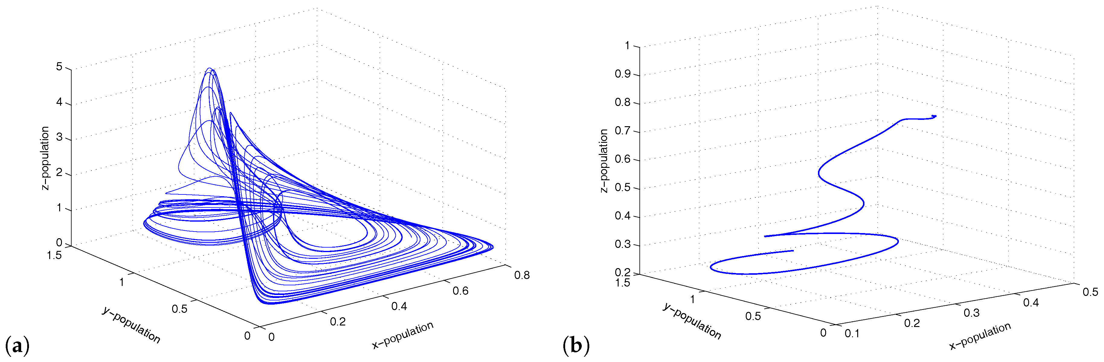
(a,b) Chaotic oscillations and stable focus of the system given by Equation (3) for and , respectively.
Figure 1.
(a,b) Chaotic oscillations and stable focus of the system given by Equation (3) for and , respectively.

Figure 2.
Bifurcation diagram for and populations of the coupled Hastings–Powell (HP)–HP system corresponding to the bifurcating parameter k, where .
Figure 2.
Bifurcation diagram for and populations of the coupled Hastings–Powell (HP)–HP system corresponding to the bifurcating parameter k, where .

Figure 3.
Figure shows stable dynamics of the coupled system given by Equation (4) for .
Figure 3.
Figure shows stable dynamics of the coupled system given by Equation (4) for .

Figure 4.
Figure shows chaotic oscillations and stable focus for and , respectively.

Figure 5.
Bifurcation diagram of the top-predator populations of the coupled system corresponding to the bifurcating parameter k, where .
Figure 5.
Bifurcation diagram of the top-predator populations of the coupled system corresponding to the bifurcating parameter k, where .
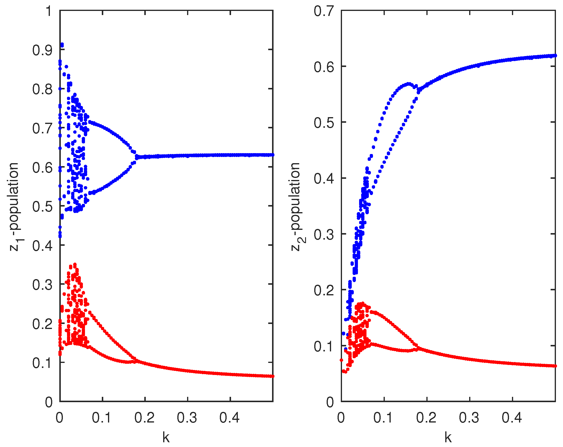
Figure 6.
Figure shows limit cycle oscillations of the coupled system for .

Figure 7.
(a,b) Chaotic oscillations and stable focus of the system given by Equation (8) for and , respectively.
Figure 7.
(a,b) Chaotic oscillations and stable focus of the system given by Equation (8) for and , respectively.

Figure 8.
Bifurcation diagram for and populations of the coupled Upadhyay–Rai (UR)–UR system corresponding to the bifurcating parameter k, where .
Figure 8.
Bifurcation diagram for and populations of the coupled Upadhyay–Rai (UR)–UR system corresponding to the bifurcating parameter k, where .

Figure 9.
The figure shows stable dynamics of the coupled system given by Equation (9) for .
Figure 9.
The figure shows stable dynamics of the coupled system given by Equation (9) for .

Figure 10.
(a,b) Chaotic oscillations and stable focus of the system given by Equation (11) for and , respectively.
Figure 10.
(a,b) Chaotic oscillations and stable focus of the system given by Equation (11) for and , respectively.

Figure 11.
Bifurcation diagram for and populations of the coupled Priyadarshi–Gakkhar (PG)–PG system given by Equation (12) corresponding to the bifurcating parameter k, where .
Figure 11.
Bifurcation diagram for and populations of the coupled Priyadarshi–Gakkhar (PG)–PG system given by Equation (12) corresponding to the bifurcating parameter k, where .
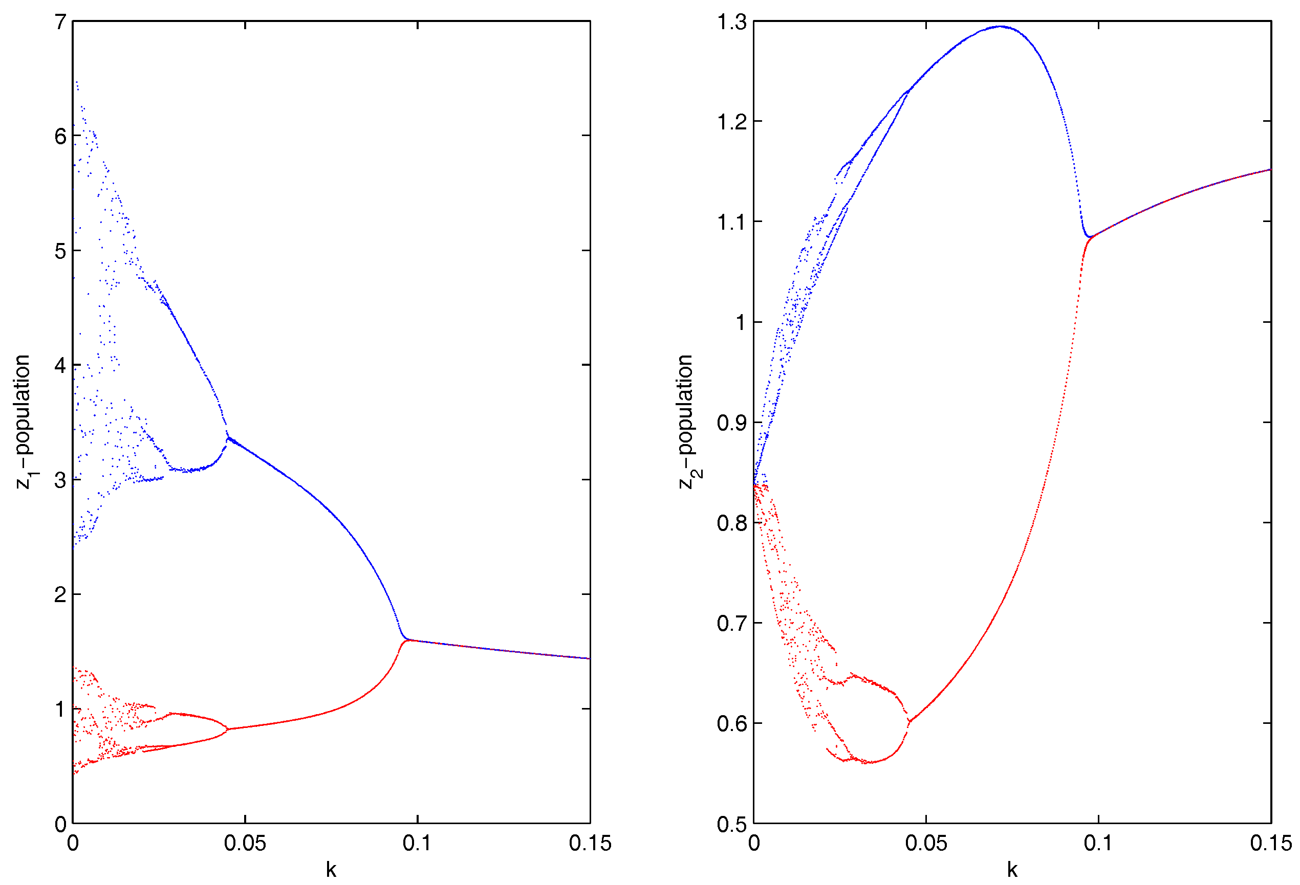
Figure 12.
The figure shows stable dynamics of the coupled system given by Equation (12) for .
Figure 12.
The figure shows stable dynamics of the coupled system given by Equation (12) for .

© 2018 by the authors. Licensee MDPI, Basel, Switzerland. This article is an open access article distributed under the terms and conditions of the Creative Commons Attribution (CC BY) license (http://creativecommons.org/licenses/by/4.0/).
Share and Cite
MDPI and ACS Style
Pal, N.; Samanta, S.; Martcheva, M.; Chattopadhyay, J. Role of Bi-Directional Migration in Two Similar Types of Ecosystems. Mathematics 2018, 6, 36. https://doi.org/10.3390/math6030036
AMA Style
Pal N, Samanta S, Martcheva M, Chattopadhyay J. Role of Bi-Directional Migration in Two Similar Types of Ecosystems. Mathematics. 2018; 6(3):36. https://doi.org/10.3390/math6030036
Chicago/Turabian StylePal, Nikhil, Sudip Samanta, Maia Martcheva, and Joydev Chattopadhyay. 2018. "Role of Bi-Directional Migration in Two Similar Types of Ecosystems" Mathematics 6, no. 3: 36. https://doi.org/10.3390/math6030036
Note that from the first issue of 2016, this journal uses article numbers instead of page numbers. See further details here.