Best Approximation of the Fractional Semi-Derivative Operator by Exponential Series


Institute of Mathematics and Information Technologies, Volgograd State University, Volgograd 400062, Russia
*
Author to whom correspondence should be addressed.
Mathematics 2018, 6(1), 12; https://doi.org/10.3390/math6010012
Submission received: 30 November 2017
/
Revised: 11 January 2018
/
Accepted: 12 January 2018
/
Published: 16 January 2018
(This article belongs to the Special Issue Fractional Calculus: Theory and Applications)
Abstract
:A significant reduction in the time required to obtain an estimate of the mean frequency of the spectrum of Doppler signals when seeking to measure the instantaneous velocity of dangerous near-Earth cosmic objects (NEO) is an important task being developed to counter the threat from asteroids. Spectral analysis methods have shown that the coordinate of the centroid of the Doppler signal spectrum can be found by using operations in the time domain without spectral processing. At the same time, an increase in the speed of resolving the algorithm for estimating the mean frequency of the spectrum is achieved by using fractional differentiation without spectral processing. Thus, an accurate estimate of location of the centroid for the spectrum of Doppler signals can be obtained in the time domain as the signal arrives. This paper considers the implementation of a fractional-differentiating filter of the order of ½ by a set of automation astatic transfer elements, which greatly simplifies practical implementation. Real technical devices have the ultimate time delay, albeit small in comparison with the duration of the signal. As a result, the real filter will process the signal with some error. In accordance with this, this paper introduces and uses the concept of a “pre-derivative” of ½ of magnitude. An optimal algorithm for realizing the structure of the filter is proposed based on the criterion of minimum mean square error. Relations are obtained for the quadrature coefficients that determine the structure of the filter.
1. Introduction
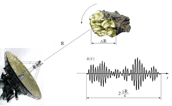
A number of technical problems require the estimation of the parameters of the spectrum of broadband signals in real time. For example, in radar, the central frequency of the Doppler signal spectrum determines the radial component of the speed of the moving object and is necessary for prediction of its trajectory. In particular, this issue refers to Doppler radar systems that measure the spectral characteristics of beats of a probing and reflected signal. Accurate and rapid measurement of these parameters, in this case, is a necessary condition for effective operation of such systems. However, in order to estimate the parameters of the reflected signal spectrum, the use of spectral analysis does not always satisfy operational requirements. For example, the spectrum of the Doppler signal can be broadened by the motion of individual points of the object with different velocities. In the case when the various points of the object forming the reflected signal move with different velocities (for example, when the object rotates), the reflected signal can have a wide spectrum of Doppler frequencies corresponding to the spectrum of the reflecting point velocities on its surface. In such a case, the centroid of the energy spectrum of the Doppler signal is used as the Doppler frequency in the radar, which remains a stable characteristic corresponding to the motion of the center of mass of the moving object. A complex movement of an object can take place if the object maneuvers. For uncontrolled objects, in particular, asteroids, tumbling (rotation with respect to all three axes with incommensurable angular velocities) is a common phenomenon when moving along a ballistic trajectory [1]. This reduces the accuracy of estimating the instantaneous speed of the object and complicates the forecast of its trajectory. The priority of mankind to counteract the threat from near-Earth cosmic objects (NEO’s) explains the importance of solving the subtask of ultra-fast and ultra-precise determination of the speed of a fast asteroid [2].
A fast and accurate forecast of the trajectory of a dangerous cosmic object is necessary for calculating the point of encounter for weapons to destroy such an object. Forecasting the trajectory is undertaken by measuring the speed of the object based on the analysis of the Doppler frequency shift of the reflected radar signal.
Increasing the accuracy and speed of measuring the frequency of the Doppler signal is a prerequisite for the effective operation of space-based radar systems. At the final stage of the weapons’ approach to the object, the parameters of the asteroid’s motion must be measured quickly. At velocities of cosmic objects of several tens of km/s, the error price multiplies many times, and the requirements for accuracy must be maximized.
It was shown in [3,4] that an estimate of the velocity of the “average” point of a fast moving asteroid can be reduced to a calculation of the derivative of order ½ from the so-called “Doppler signal”, that is, the beat signal of the reflected and probing signals. On the basis of this, an algorithm for the operation of a fractional-differentiating filter (FDF) of order ½ has been proposed, which allows for the estimation of the centroid of the spectrum of the input signal to be obtained in real time without spectral processing. It has also been shown that the use of such a fractal-processing algorithm makes it possible to increase the rate by which an estimate can be obtained by up to six orders of magnitude [4].
Of course, modern signal-processing tools should be designed as digital, given obvious progress in the development of digital devices, and questions about the analog methods. The characteristics of digital filters are absolutely stable, while the parameters of analog filters are unstable and depend on external conditions.
Nevertheless, models of analog devices usually precede the construction of digital models. Analog algorithms are more obvious than digital ones. The analog filter in this problem is interesting in that it allows for real-time signal processing, i.e., at the rate of input of the input signal.
In the present paper, using an analog FDF as an example, we consider its possible use by simple technical means in the form of a set of operations realized by simple elements of—astatic transfer elements of the first order. We show that, mathematically, the structure of the FDF can be represented by a linear approximation of the kernel of the fractional derivative operator of the order of ½ by decaying exponents. We propose an optimal realization of the structure of the FDF by the criterion of minimum mean square error.
The problem considered in the present paper belongs to that class of problems pertaining to the recognition of signal singularities. We note the rapid growth of the development of algorithms using fractional differentiation, specifically in the field of artificial intelligence. These include, for example, image-processing algorithms [5], the identification of image features [6,7,8], and computer [9,10,11] and experimental [12,13] implementation of fractal proportional-integral-derivative (PID) controllers for industrial control systems.
2. The Possibility of Using Fractal Signal Processing
As a signal , we consider a class of Lebesgue measurable functions on a set , . In other words, for functions , the inequality must hold, where . The function corresponds to the spectral density of the signal amplitude (spectrum) . Here, the symbol denotes the Fourier transform of the signal.
In the theory of signals, the method of moments [14] (pp. 135–136) is widely used to estimate the parameters of the spectrum, according to which the mean frequency and effective width of the signal spectrum on the positive half-axis of frequencies is defined as the centroid and twice the radius of inertia (twice the standard deviation) of the energy spectrum of the signal (see Figure 1):
In the case of expanding the spectrum of Doppler frequencies, it can be agreed that the “average” speed of the object is estimated from the position of the centroid of the spectrum [15] whose definition is given by the ratio:
Calculations using Equation (1) require a sufficiently long time for the observation of the signal and its processing, since processing uses the procedure for calculating the spectrum , which from the computational point of view is quite laborious. With the number of signal samples, the calculation of the spectrum in the most economical case will require the number of multiplications by the fast Fourier transform (FFT) technique. To this, we additionally require multiplications in order to calculate the integrals in the numerator and denominator in the fraction (1). In addition, in order to carry out these calculations it is necessary to first obtain the entire signal (all samples), which introduces an additional delay in obtaining an estimate. Moreover, such an algorithm requires a fairly large amount of working memory for counts of the spectrum. In this case, it is advantageous to have a flow algorithm that allows for the calculation of the numerator and denominator in Equation (1) in real time as the signal arrives. This condition is satisfied by the Duhamel integral calculation algorithm, which can be realized using a transversal filter that processes a signal in the time domain in real time. This allows us to calculate the numerator and denominator in Equation (1) at the end of the signal.
It has been shown in [3,4] that the right-hand side of Equation (1) can be represented by the ratio of the square of the fractional derivative to the square of the signal’s norm (energy), which allows for us to find the centroid of the spectrum without using the Fourier transform:
Here is the operator of the fractional Liouville derivative of half-integer order [16]
which we further refer to as the semiderivative operator in accordance with the terminology that has been accepted in the literature. The denominator of the fraction in Equation (2) is derived using Parseval’s equation [14] (p. 140) in the transition from the frequency domain to the time domain:
Similarly, on the basis of Parseval’s equality, the numerator of the fraction in (2) is also transformed:
where is the imaginary unit. From this, it follows that in order to calculate the centroid of the spectrum, it is necessary to calculate the square of the norm of the fractional derivative of the order of ½ and the signal energy.
The semi-derivative operator must satisfy the following condition:
Equation (6) shows that the fractional derivative can be calculated using linear FDF. The action of the fractional derivative operator according to Equation (6) is interpreted as the convolution of the investigated signal with the following function
which is usually called the pulse response of the FDF. The pulse response (7) is identical to the kernel of the fractional differentiation operator.
It follows from Equation (2) that for a limited observation interval of signal (), the processing time can be substantially reduced if we calculate the fractional derivative of the order of ½ in real time [3,4]. Estimating the location of the centroid of the spectrum (2) can be undertaken without spectral processing as the reflected signal reaches the detector and is obtained at the end of the observation interval . For example, in the problem of the rapid estimation of the radial velocity of a potentially dangerous near-Earth asteroid, the real computational speed can be increased by a million times [4].
In fact, for a space object with a diameter of ~100 m and a rotation period of ~10 min, the width of the velocity spectrum amounts to ~1 m/s, which corresponds to the width of the Doppler spectrum in the X band ~50 Hz. In this case, the average Doppler frequency at a speed of 30 km/s is ~2 MHz; the signal sampling frequency should be appropriately selected as >4 MHz ( 0.1 мs).
For high-speed resolution (~0.01 m/s or higher), it is necessary to measure the Doppler frequency with an accuracy of ~0.5 Hz. With a Doppler duration of ~0.1 s, this will require processing of the signal samples.
A standard calculation using the FFT method will require multiplication operations. For a processor with a performance of 1 Mflops, this will take about 20 s, while the signal delay in the filter for the filter of order is only s. Thus, the gain in speed will be more than six orders. Time costs will be comparable only when using the FFT method on processors with a performance of several teraflops, which is economically unprofitable and technically difficult to implement.
Thus, it is important to find the optimal algorithm for an approximate calculation of the fractional derivative of the signal (maximum accuracy with a minimum of computational operation). If fractional differentiation is performed on analog devices, then the algorithm simultaneously determines the design of real devices. The present paper is devoted to the search for the quadrature of the highest degree of accuracy for finding the approximate value of the fractional semi-derivative.
We emphasize that we do not construct an n-point quadrature of the highest degree of accuracy for calculating the semi-derivative in which the semi-derivative is approximated by the weighted sum of the values of the integrand at different nodes. Such a problem was solved long ago [17,18]. Instead, we find the best approximation precisely for the kernel of the fractional derivative operator, and the calculation of the semi-derivative by the quadrature formula deduced by us reduces to the sum of integrals contained as weight-function damped exponentials.
3. The Pulse Response Characteristic of the Liouville Semi-Derivative
By virtue of the linearity property of the fractional differentiation operator and the difference kernel, expression (6) can be written as the Duhamel integral [14] (p. 142),
and this means that the fractional differentiation operator can be realized as a linear stationary FDF with specified characteristics. The general requirements imposed on the filter are expressed by the conditions (9) and (10).
Among the mandatory requirements is the condition of causality of the impulse response
which has already been taken into account in its definition in Equation (8).
The specific form of the pulse response is determined by the method of specifying a fractional derivative. In [3,4], the definition of a fractional Riemann-Liouville derivative was used. Here we confine ourselves to its particular limiting case, the Liouville derivative [16]
The Liouville derivative (3) has more habitual and evident properties, such as the identity vanishing of the derivative of a constant. The latter, as follows from Equation (8), implies another condition on the pulse response
An explicit expression for the pulse response of the Liouville operator of a semi-derivative is presented in [3,4]:
Here is the Dirac function, and is the Heaviside function. Since this expression was originally derived in an article in a hard-to-get edition [19], we reiterate its derivation below.
Definition 1.
Let . Then the left-sided Liouville pre-derivative of order ½ is defined by
We call the real quantity the parameter of the pre-derivative.
Definition 2.
The Liouville fractional derivative of order ½ (see Equation (3)) is then defined as the limit of sequence of the Liouville pre-derivatives:
Theorem 1.
The pulse response of the Liouville operator of a semi-derivative (13) is given by Equation (11).
Proof.
Differentiating the integral with a variable upper limit on the rhs of Equation (12) with respect to ,
and using the definition (6), we find an expression for the pulse response of the pre-derivative in the form
Passing to the limit , we confirm that Equation (11) is satisfied.
4. Approximation of Operator Kernel of Fractional Pre-Derivative by Superposition of Damped Exponentials
For the practical implementation of analog FDF, it is desirable to use the simplest technical means. These are physical elements with pulse characteristics in the form of damped exponentials that are the first-order astatic transfer elements [20]. The time of the pulse response decay from the physical point of view corresponds to the memory time of the physical element.
We construct the best approximation of the impulse response of a FDF of the order of ½ by a linear combination of damped exponentials. We will take into account the fact that, in the practical implementation of differentiating or integrating filters, one always has to have finite systems in which there is a finite delay time . The magnitude of the time delay is sufficiently small and is determined by the signal delay in the input circuits of the analog device. Usually it is a fraction of a microsecond, which is commensurate with the clock interval of digital signal processing processors, and is small when compared to the time of signal processing by the filter. As digital technology develops, the value of will only decrease.
Our task is to approximate the component of expression (15), which has the form of a damped power function,
by a set of damped exponentials on the interval .
The direct Laplace transform of a function ,
is the expansion of a function over an infinite set (continuum) of exponentials. The problem is reduced to finding a quadrature formula containing a finite number of exponentials for an approximate presentation of ,
instead of the true representation (the continuum of exponentials). Here, is the remainder term, , the weight coefficients, and , the nodes of the approximating quadrature formula.
Let us change a variable. We introduce the function:
Then, (17) can be rewritten in the form:
where is the inverse of (19).
From the condition for the existence of the Laplace integral,
and from definition (19), it follows that,
and the variable itself is defined on the interval .
The maximum accuracy when approximating the integral (20) by a quadrature of type (18), as we know, can be achieved using the Gaussian quadrature of the highest degree of accuracy [21]. To achieve maximum accuracy, when integrating the integral over a finite interval with a fixed number of nodes , the quadrature formula follows as nodes, where ; we take the nodes of the Legendre polynomials, and as weight coefficients and some functional combinations of them. In this case, of course, it is necessary to transform the segment on which the Legendre polynomials are defined into a segment . The nodes and weight coefficients of the Gauss–Legendre quadrature formulas can be found in the reference books [22].
We note that the inverse Laplace transform,
and the relation resulting from (19),
allow for us to establish a connection between and if (23) is integrated over :
For in a particular form (16), the Laplace transform is known:
Here, is the gamma function. Integrating (24), we find:
The function that is found increases monotonically from zero to the maximum value:
Unfortunately, the function according to (27), although continuous on the interval , is non-smooth. When it behaves like , so does not even have the first derivative. According to the standard estimate [22],
where is the majorant estimate of the absolute value of the derivative,
the Gauss-Legendre quadrature will not show rapid convergence with an increasing number of nodes.
5. Test Results
In numerical calculations, a harmonic signal with a constant amplitude and phase was considered as a model. The accuracy of the approximation was estimated by the mean-square error:
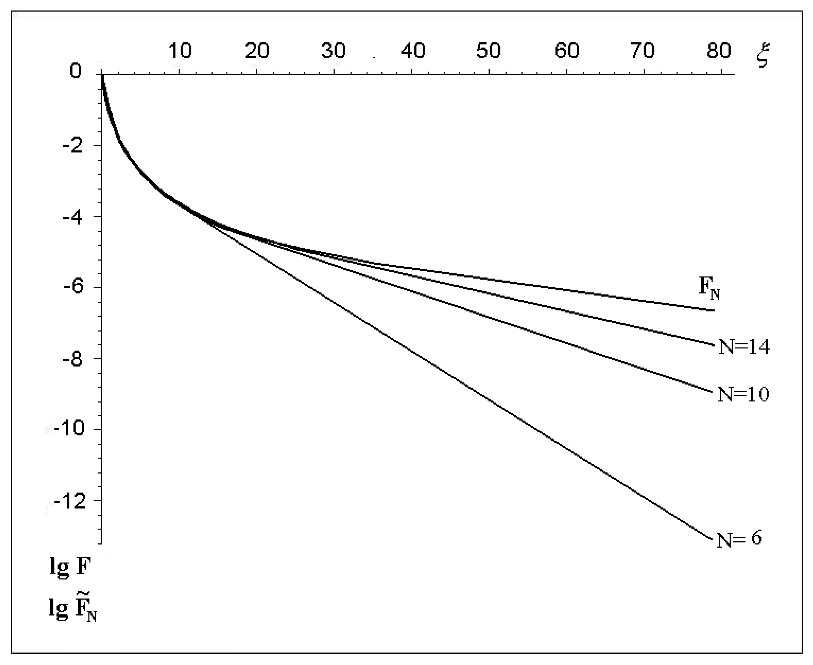
Figure 2 demonstrates on a logarithmic scale the approximated function (upper curve), and approximating functions , successively approaching at = 6, 10, 14.
The calculations show that decreases with growth , but its tendency to zero is relatively slow because the exponents decrease faster than a polynomial of any degree. The same calculations show that to achieve acceptable accuracy in radio engineering of 1% (i.e., ), it is necessary to take = 18 elements. It should be borne in mind that the elements making up a real filter include errors due to the imperfection of their manufacture. In this case, in practice the error introduced by each element will be accumulated separately and, therefore, it is not profitable to build a filter from such a large number of elements ( = 18).
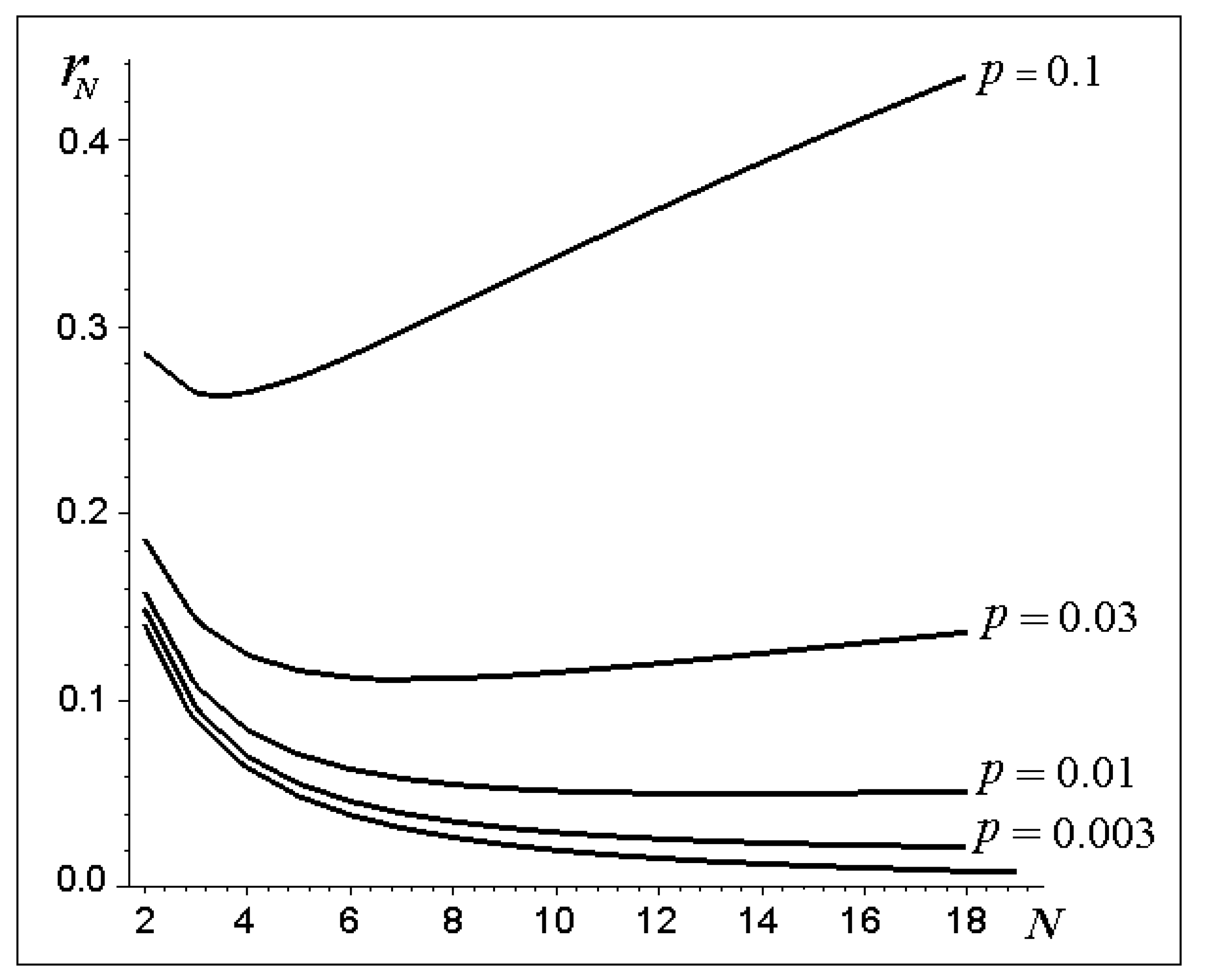
Consider the optimization of the number of elements in more detail. Let each element be characterized by a relative error in the manufacture of the device. It is natural to expect the total error introduced by elements to be defined as a statistical error proportional to the root of the number of elements. Then, the total error of the FDF approximation will be:
Figure 3 presents the graphs of the total error . If the permissible error of the device is = 0.01, then, as follows from the figure, the minimum of the total error as a function of the number of elements is reached approximately at = 12. The minimum is thus flat, and this means that when decreasing the number of elements, the error will change insignificantly. Hence it follows that for almost the same accuracy of approximation it is economically more advantageous to use 6–8 elements to construct the FDF.
6. Conclusions
The radial velocity of fast asteroids that pose a danger to the Earth (speeds of tens of kilometers per second) can be accurately measured by means of radar by estimating the centroid of the Doppler signal spectrum.
An increase in the speed of the algorithm used for estimating the average frequency of the spectrum of the Doppler signals in the time domain as the signal is received can be achieved by using fractional differentiation without spectral processing. Thus, an accurate estimate of the centroid of the signal spectrum can be obtained almost immediately after the arrival of the signal.
The approximation of the impulse response of an analog FDF by a quadrature of the highest degree of accuracy is constructed in this paper. The kernel of the fractional pre-derivative operator is approximated by the sum of the damped exponentials. The calculation is made for FDF, as composed of the first-order astatic elements that are common in engineering, which greatly simplifies practical implementation. Relations are obtained for the quadrature coefficients that determine the structure of the FDF. The number of approximation nodes corresponds to the number of elements making up the filter. There is convergence: with the increasing number of nodes used, the accuracy of the approximation can be made arbitrarily high. The accuracy of the procedure for approximate fractional differentiation, based on the use of an approximating quadrature on the example of a function, is proved using the analytic expression of the Liouville semi-derivative for which it is known (the harmonic signal).
The problem of optimizing the analog FDF circuit, composed of first-order astatic elements, has been solved. In order to limit the number of elements used, and in order to achieve the specified accuracy, an optimal number of elements is found for a given error of each. It is shown that to achieve a precision characteristic in engineering of 99%, the optimal scheme is from elements.
7. Patents
The method for estimating the mean frequency of Doppler signals reflected by fast maneuvering targets in real time using fractional differentiation operations is protected by the Russian Federation Patent [Zakharchenko V.D. Method for estimating the mean frequency of broadband Doppler signals—RF Patent No. 2114440, 27.06.98].
Acknowledgments
This study was supported by the grant 15-47-02438-r-povolzhie_a from the Russian Foundation for Basic Research.
Author Contributions
Vladimir D. Zakharchenko suggested an idea of fractional differential analog filter composed of 1st-order lag elements; Ilya G. Kovalenko constructed an exponential series expansion; both co-wrote the paper.
Conflicts of Interest
The authors declare no conflict of interest.
References
- Hatch, P.; Wiegert, P.A. On the rotation rates and axis ratios of the smallest known near-Earth asteroids—The archetypes of the Asteroid Redirect Mission targets. Planet. Space Sci. 2015, 111, 100–104. [Google Scholar] [CrossRef]
- National Near-Earth Object Preparedness Strategy (December 2016). Available online: https://www.nasa.gov/sites/default/files/atoms/files/national_near-earth_object_preparedness_strategy_tagged.pdf (accessed on 29 November 2017).
- Zakharchenko, V.D.; Kovalenko, I.G. Estimation of radial velocity of objects using fractional differentiation of Doppler radar signal. In Proceedings of the 23rd Int. Crimean Conference “Microwave & Telecommunication Technology” (CriMiCo’2013), Sevastopol, Ukraine, 9–13 September 2013; Weber Publishing: Sevastopol, Ukraine, 2013; Volume 2, pp. 1120–1121. [Google Scholar]
- Zakharchenko, V.D.; Kovalenko, I.G. On protecting the planet against cosmic attack: ultrafast real-time estimate of the asteroid’s radial velocity. Acta Astronaut. 2014, 98, 158–162. [Google Scholar] [CrossRef]
- Khanna, S.; Chandrasekaran, V. Fractional derivative filter for image contrast enhancement with order prediction. In Proceedings of the IET Conference on Image Processing (IPR 2012), London, UK, 3–4 July 2012; Curran Associates, Inc.: Red Hook, NY, USA, 2012; pp. 73–78, ISBN 978-1-62276-267-5. [Google Scholar] [CrossRef]
- Mathieu, B.; Melchior, P.; Oustaloup, A.; Ceyral, C. Fractional differentiation for edge detection. Signal Process. 2003, 83, 2421–2432. [Google Scholar] [CrossRef]
- Pu, Y.; Wang, W.-X.; Zhou, J.-L.; Wang, Y.-Y.; Jia, H.-D. Fractional Differential Approach to Detecting Textural Features of Digital Image and Its Fractional Differential Filter Implementation. Sci. China Ser. F Inf. Sci. 2008, 51, 1319–1339. [Google Scholar] [CrossRef]
- Xu, X.; Dai, F.; Long, J.; Guo, W. Fractional Differentiation-based Image Feature Extraction. Int. J. Signal Proc. Image Proc. Pattern Recogn. 2014, 7, 51–64. [Google Scholar] [CrossRef]
- Luo, Y.; Chen, Y.Q. Fractional order [proportional derivative] controller for a class of fractional order systems. Automatica 2009, 45, 2446–2450. [Google Scholar] [CrossRef]
- Biswas, A.; Das, S.; Abraham, A.; Dasgupta, S. Design of fractional-order PIλDμ controllers with an improved differential evolution. Eng. Appl. Artif. Intell. 2009, 22, 343–350. [Google Scholar] [CrossRef]
- Luo, Y.; Chen, Y.Q.; Wang, C.Y.; Pi, Y.G. Tuning fractional order proportional integral controllers for fractional order systems. J. Process Control 2010, 20, 823–831. [Google Scholar] [CrossRef]
- Monje, C.A.; Vinagre, B.M.; Feliu, V.; Chen, Y.Q. Tuning and auto-tuning of fractional order controllers for industry applications. Control Eng. Pract. 2008, 16, 798–812. [Google Scholar] [CrossRef] [Green Version]
- Luo, Y.; Chen, Y.Q.; Pi, Y. Experimental study of fractional order proportional derivative controller synthesis for fractional order systems. Mechatronics 2011, 21, 204–214. [Google Scholar] [CrossRef]
- Franks, L.E. Signal Theory; Prentice-Hall: Upper Saddle River, NJ, USA, 1969. [Google Scholar]
- Gonorovskii, I.S. Radio Circuits and Signals, 5th ed.; Drofa: Moscow, Russia, 2006; pp. 69–73. ISBN 5-7107-7985-7. (In Russian) [Google Scholar]
- Samko, S.; Kilbas, A.; Marichev, O. Fractional Integrals and Derivatives. Theory and Application; Gordon & Breach Sci. Publishers: Philadelphia, PA, USA, 1993; p. 95. ISBN 2881248640. [Google Scholar]
- Lether, F.G. Quadrature rules for approximating semi-integrals and semiderivatives. J. Comput. Appl. Math. 1987, 17, 115–129. [Google Scholar] [CrossRef]
- Acharya, M.; Mohapatra, S.N.; Acharya, B.P. On Numerical Evaluation of Fractional Integrals. Appl. Math. Sci. 2011, 5, 1401–1407. [Google Scholar]
- Zakharchenko, V.D. Mean frequency of Doppler signals estimate by the method of fractional differentiation. Phys. Wave Process. Radiotech. Syst. 1999, 2, 39–41. (In Russian) [Google Scholar]
- Unbehauen, H. Description of Continuous Linear Time-Invariant Systems in Frequency Domain. In Control Systems, Robotics, and Automation; Unbehauen, H., Ed.; EOLSS Publishers Co. Ltd.: Abu Dhabi, UAE, 2009; Volume 1, pp. 164–189. ISBN 1848265905. [Google Scholar]
- Hildebrand, F.B. Introduction to Numerical Analysis, 2nd ed.; McGraw-Hill: New York, NY, USA, 1974; pp. 390–394. ISBN 0-07-028761-9. [Google Scholar]
- Kahaner, D.; Moler, C.; Nash, S. Numerical Methods and Software; Prentice Hall: Bergen County, NJ, USA, 1989; p. 146. ISBN 978-0-13-627258-8. [Google Scholar]
Figure 1.
Determination of the parameters of the spectrum and of the Doppler signal by the method of moments. is the velocity distribution of the reflecting elements of the object’s surface.
Figure 1.
Determination of the parameters of the spectrum and of the Doppler signal by the method of moments. is the velocity distribution of the reflecting elements of the object’s surface.
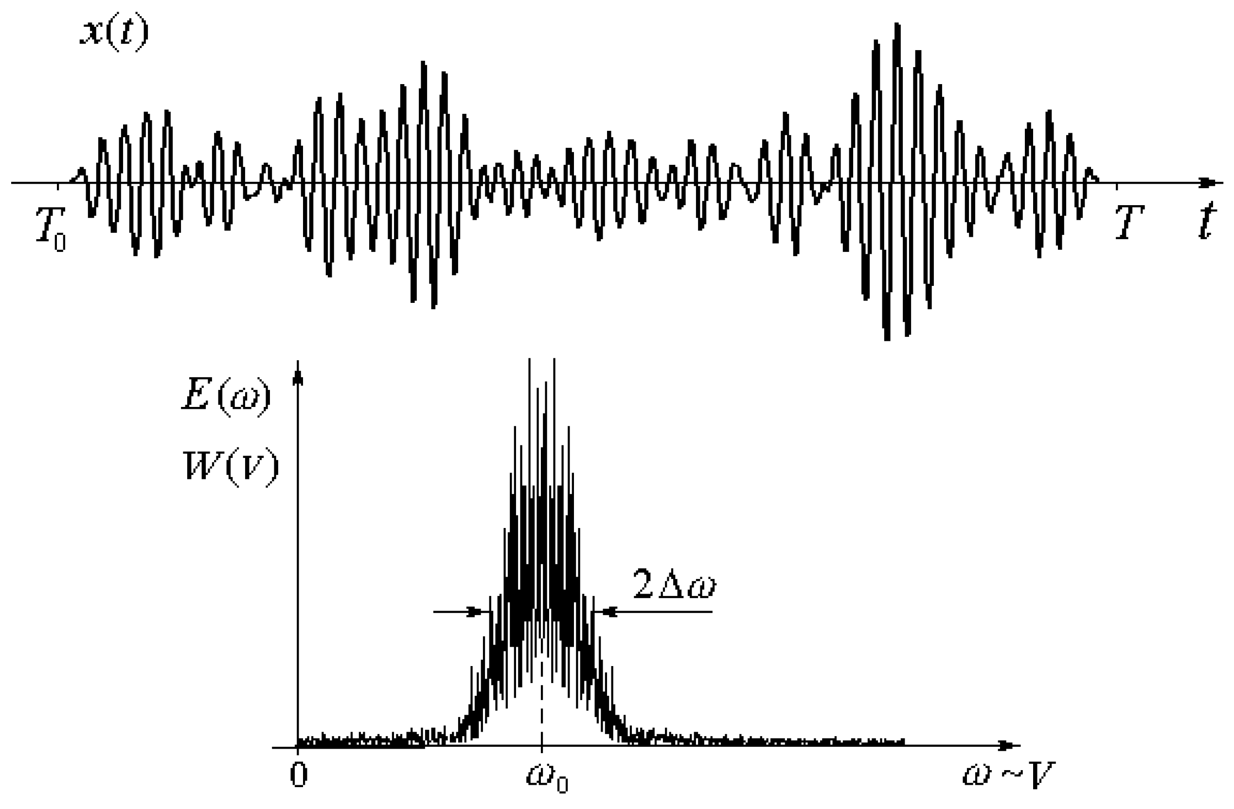
Figure 2.
Dependence of the approximated function and approximating functions .

Figure 3.
Graphs of functions of total errors . The lower curve corresponds to the rootmean-square error . From the bottom up are the curves corresponding to the errors of the device = 0.003, 0.01, 0.03, 0.1.
Figure 3.
Graphs of functions of total errors . The lower curve corresponds to the rootmean-square error . From the bottom up are the curves corresponding to the errors of the device = 0.003, 0.01, 0.03, 0.1.

© 2018 by the authors. Licensee MDPI, Basel, Switzerland. This article is an open access article distributed under the terms and conditions of the Creative Commons Attribution (CC BY) license (http://creativecommons.org/licenses/by/4.0/).
Share and Cite
MDPI and ACS Style
Zakharchenko, V.D.; Kovalenko, I.G. Best Approximation of the Fractional Semi-Derivative Operator by Exponential Series. Mathematics 2018, 6, 12. https://doi.org/10.3390/math6010012
AMA Style
Zakharchenko VD, Kovalenko IG. Best Approximation of the Fractional Semi-Derivative Operator by Exponential Series. Mathematics. 2018; 6(1):12. https://doi.org/10.3390/math6010012
Chicago/Turabian StyleZakharchenko, Vladimir D., and Ilya G. Kovalenko. 2018. "Best Approximation of the Fractional Semi-Derivative Operator by Exponential Series" Mathematics 6, no. 1: 12. https://doi.org/10.3390/math6010012
Note that from the first issue of 2016, this journal uses article numbers instead of page numbers. See further details here.