
Fractional Schrödinger Equation in the Presence of the Linear Potential

Institut für Lasertechnologien in der Medizin und Meßtechnik an der Universität Ulm, Helmholtzstr. 12, D-89081 Ulm, Germany
*
Author to whom correspondence should be addressed.
Mathematics 2016, 4(2), 31; https://doi.org/10.3390/math4020031
Submission received: 24 March 2016
/
Revised: 18 April 2016
/
Accepted: 21 April 2016
/
Published: 4 May 2016
(This article belongs to the Special Issue Fractional Differential and Difference Equations)
Abstract
:In this paper, we consider the time-dependent Schrödinger equation:
with the Riesz space-fractional derivative of order in the presence of the linear potential . The wave function to the one-dimensional Schrödinger equation in momentum space is given in closed form allowing the determination of other measurable quantities such as the mean square displacement. Analytical solutions are derived for the relevant case of , which are useable for studying the propagation of wave packets that undergo spreading and splitting. We furthermore address the two-dimensional space-fractional Schrödinger equation under consideration of the potential including the free particle case. The derived equations are illustrated in different ways and verified by comparisons with a recently proposed numerical approach.
1. Introduction
The time-dependent Schrödinger equation is a fundamental equation in quantum mechanics for studying the dynamics and evolution of wave packets over time. Several years ago, the classical Schrödinger equation has been generalized to a fractional partial differential equation that takes into account the Riesz space-fractional derivative instead of the conventional Laplacian [1,2]. Apart from quantum mechanics, there are many other equations occurring in science that have been reconsidered in terms of fractional derivatives such as the diffusion-wave equation [3,4,5,6], the Langevin equation [7] or the radiative transport equation [8]. Analytical solutions to fractional differential equations are, in general, not available in terms of elementary functions. As an example, the fundamental solution to the Schrödinger equation for a free particle can only be written in closed form under consideration of the Fox H-function [9]. Very recently, the space-fractional Schrödinger equation has been employed for studying the propagation dynamics of wave packets in the presence of the harmonic potential [10] as well as of the free particle [11]. In addition, the fractional Schrödinger equation subject to a periodic -symmetric potential has been used to investigate the conical diffraction of a light beam [12]. An optical realization of the space-fractional Schrödinger equation, based on transverse light dynamics in aspherical optical cavities, has been recently proposed in the study [13]. Besides the free particle and the harmonic potential, the case of a linear potential is also a fundamental problem in quantum mechanics that can be treated and solved analytically [14,15]. In this context, we refer to the paper [16] dealing with the nonlinear Schrödinger equation in the presence of uniform acceleration. We additionally note on the time-dependent Schrödinger equation with a nonlocal term that has been analyzed in the publication [17].
In this article, we consider the time-dependent Schrödinger equation with the Riesz space-fractional derivative of order in the presence of the linear potential. In the one-dimensional (1D) case, the wave function in momentum space is derived for an arbitrary fractional order α in closed form, which allows the determination of other important quantities such as the mean square displacement (MSD). For the case of , we provide some explicit analytical solutions useable for studying the time evolution of wave packets that undergo both spreading and splitting. We additionally address the space-fractional Schrödinger equation in two spatial dimensions. The obtained equations are illustrated in different ways and partly verified by comparisons with a recently proposed numerical approach.
2. 1D Space-Fractional Schrödinger Equation
The 1D space-fractional Schrödinger equation in the presence of the linear potential is given by
where is the wave function, is the order of the Riesz space-fractional derivative and . The nonlocal operator occurring in Equation (1) is defined in the sense of [18]
with being the Fourier transform of . Alternatively, it can also be defined directly in real space in terms of the left- and right-sided Riemann-Liouville derivatives [19]. In this section, Equation (1) is considered under the initial and boundary conditions
where is the initial wave packet that is normalized according to . The corresponding Schrödinger equation in momentum space is given by
where . In order to solve this equation, we introduce a wave function of the form , where φ and u are unknown. Inserting this function into Equation (4) results in
where denotes the first derivative of the unknown function u. Comparing both sides of Equation (5) leads to the equation
which is solved by the function
with C being an arbitrary constant. The unknown quantity u can be found by employing the initial condition according to
Therefore, the general solution of the Schrödinger Equation (4) in momentum space is found to be
for all . It can be seen that , which is a measure for the probability density in momentum space, is independent of the fractional order. The wave function in real space is formally given by
In general, this integral must be carried out numerically using one of the established quadrature rules. For the classical case of , the wave function can also be given in terms of the convolution
The probability density function (pdf) associated with the position of the particle is defined as . Furthermore, in view of experimental activities, the MSD is known to be an important quantity that can be computed by means of the pdf as . In our case, when is not given, the MSD can be determined from the wave function in momentum space according to
Using Equation (9), one obtains the MSD for an arbitrary initial stage as
In the following, we also want to address the case of the free particle which is obtained for . The corresponding solution in momentum space Equation (9) reduces to
However, also in this case, the wave function in real space is not available in elementary form. Instead, we have
with being Green’s function, which is given for by
The Fox H-function occurring above is defined in terms of the Mellin-Barnes integral [9]
where is the Gamma function and L denotes an appropriate integration path in the complex plane. The fundamental solution Equation (16) can be evaluated by means of the series
where . The corresponding MSD for becomes
where is the sign function. It can be verified that the MSD Equation (19) as function of time describes for all fractional orders a parabola. As an example, for the commonly applied Gaussian wave packet
one obtains in the free particle case the MSD
which exists for all . Figure 1 displays the MSD Equation (21) for different values of the fractional order.
Explicit Solutions for the Square Root of the Laplacian
In this subsection, we provide some explicit analytical solutions of Equation (1) for the order . In this case, the fractional Laplacian can be represented as [20]
where is the Hilbert transform that is defined by
and denotes the Cauchy principal value. It should be noted that, in recent time, the case of has attracted attention in the context of the propagation dynamics of wave packets under the use of the space-fractional Schrödinger equation [10,11,13]. In this study, we investigate the time evolution of the Cauchy initial wave packet
where is a measure for the beam width. We afore have to note that the time evolution of the Gaussian wave packet and the Cauchy wave packet shows a similar behavior. However, in the latter case, we are able to derive simple analytical solutions that are easy to implement and reproduce. Our starting point is the evaluation of the Fourier integral Equation (10) under consideration of the wave function Equation (9). For this, we also need the Cauchy wave packet Equation (24) in momentum space, that is . Splitting the integrand into three sections and assuming that enables the derivation of the following closed-form expression
where is the error function. Note that the case can be treated in the same manner. The associated MSD belonging to this process can be obtained from Equation (13) and summarized as
In this context, we note on the limits
In the case of the free particle, there is the possibility to provide the general solution for an arbitrary initial stage. In doing so, we need the inverse Fourier transform of the impulse response , which can be written as
Inserting this finding into Equation (15) leads to the general solution of the Schrödinger equation
In the actual case of the Cauchy initial wave packet Equation (24), we find the time evolution
which can be confirmed via Equation (25) by setting . The resulting pdf belonging to this process is
In addition, the cumulative distribution function is found to be
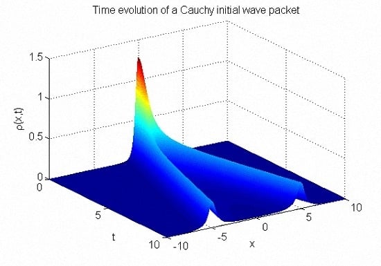
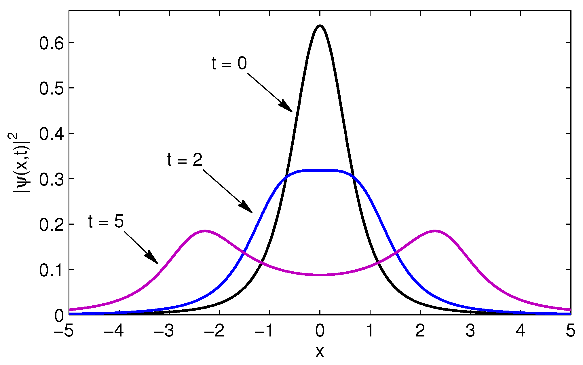
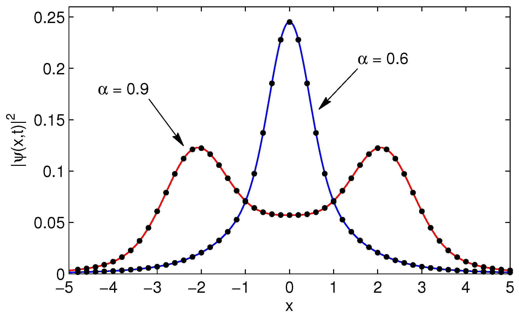
Within the classical quantum mechanics, it is known that a pdf belonging to the free particle solution typically spreads out but it does not split. However, as has been very recently shown, the pdf belonging to the space-fractional Schrödinger equation additionally undergoes splitting [11]. For the Cauchy wave packet, there is the possibility to provide some more details concerning this feature. Taking the first derivative of the pdf Equation (31) with respect to the space and setting , yields three critical positions, namely or . From the behavior of , it follows that is an absolute maximum as long as . On the other side, for time values , the position becomes a relative minimum. At the same time, we obtain two absolute maxima located at . Consequently, the probability density spreads out for , and additionally, starts to split at . For illustration purposes, Figure 2 shows the time evolution of a Cauchy initial wave packet according to Equation (31).
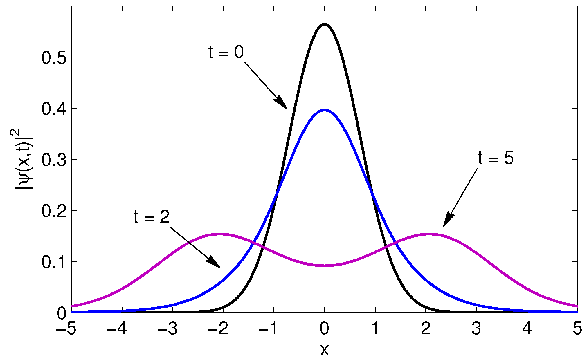
A similar behavior can be observed in the case of the Gaussian initial wave packet Equation (20), where the critical time regarding the splitting process must be determined numerically from the wave function
where is the imaginary error function and is given by Equation (20). Figure 3 displays the same situation as shown in Figure 2 for the the Gaussian initial wave packet Equation (20).
Concerning an experimental verification/realization of the derived theoretical results we refer to the recent publication [11], which proposes an optical system composed of two convex lenses and a phase mask. We furthermore note on the free particle solution to the classical Schrödinger equation. In the case of the Cauchy wave packet Equation (24), we have
where is the Faddeeva function. The corresponding MSD belonging to this process is . Figure 4 displays the time evolution of the wave function Equation (34) for the same time values considered in Figure 2. It can can be seen that the probability density indeed spreads out but it does not split.
3. 2D Space-Fractional Schrödinger Equation
The 2D space-fractional Schrödinger equation in the presence of the potential is given by
where and . Again, the 2D fractional Laplacian is most convenient defined by
where denotes the length of the wave vector that belongs to the Fourier transform . In addition, for , the 2D fractional Laplacian can be represented as
where denotes the Riesz transform [21], that maps a scalar function into a vector field according to
We note that relation Equation (37) is a generalization of the 1D differential operator Equation (22). Concerning the initial and boundary conditions in 2D, we have
where . The Schrödinger Equation (35) in momentum space becomes
where the Del operator has to be applied with regard to the Fourier variables. Similar as in 1D, we seek a wave function of the form . Inserting this ansatz into Equation (40), leads to the first order partial differential equation
In contrast to the 1D case, we are not able to solve this equation for all fractional orders in elementary form. However, for the relevant case of , an exact solution can be derived and summarized as
The solution belonging to the classical case with is less complicated and given by . Again, the unknown function u can be recovered under consideration of the initial condition such as
Therefore, we obtain the wave function in momentum space according to
In the case of the free particle with , the solution in momentum space can be given for all orders as
Moreover, if the initial wave packet exhibits rotational symmetry which implies that , the solution in real space can be evaluated by means of the inverse Hankel transform
with being the zero order Bessel function. For and , Equation (46) yields the 2D Green’s function
which can be evaluated by means of the series
where . In the case of , this relation coincides with the known result . On the other side, Green’s function for and is found to be
Based on this relation, we obtain the wave function
which is the general solution of Equation (35) for and . In the following, we investigate the time evolution of the rotationally symmetric Cauchy wave packet
which is normalized according to . Similar as in 1D, we consider the case of in detail. The desired wave function can be obtained either via the convolution Equation (50) or by means of the inverse Hankel transform Equation (46). In the latter case, we need the initial wave packet Equation (51) in momentum space, that is . The required inverse Hankel transform can be taken exactly and summarized as
The associated probability density to this wave function is given by
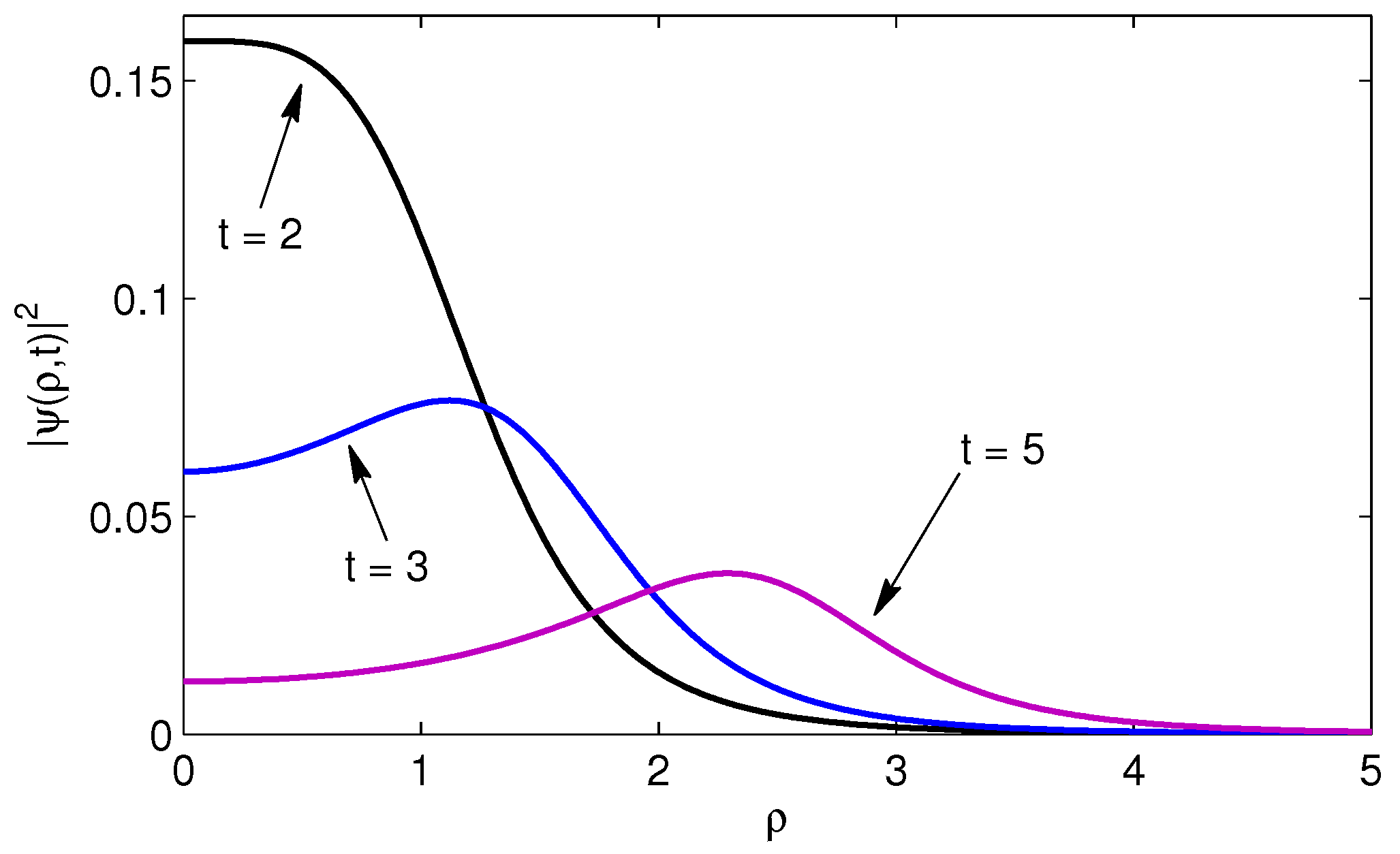
In accordance with the 1D case, the probability density in 2D also undergoes spreading and splitting. Remarkable, the probability density Equation (53) starts to split at , which is exactly the same time value as for the 1D pendant Equation (31). Figure 5 displays the time evolution of a rotationally symmetric Cauchy initial wave packet for different time values.
We note that the solution for the rotationally symmetric Gaussian wave packet can be derived in a similar manner. The required Hankel transform for evaluation of the wave function Equation (46) is given by .
4. Numerical Solution of the Fractional Schrödinger Equation
In this section, we describe a recently proposed matrix approach [22] that has been used for solving numerically the 1D space-fractional diffusion equation. In this context, we additionally refer to the recent publication [23], which takes into account the so-called Adomian decomposition method. We adopt the matrix approach in order to solve the space-fractional Schrödinger Equation (1) subject to an arbitrary potential function . Within this framework, we consider the computational domain together with the uniform grid for as well as the node spacing . Furthermore, the fractional Laplacian has to be restricted to a bounded domain. If , we have the representation
whereas for it is given by
In particular, the square root of the negative Laplacian on a bounded domain becomes
For our applications, the quantity L has to be chosen relatively large in order to obtain a reasonable model for the infinite domain. On the other side, the matrix approach is designed for solving the fractional Schrödinger on a bounded domain, where analytical solutions are typically not available. The key point here is the approximation of the fractional Laplacian by means of the fractional centered difference [22]
which can be applied for all . The corresponding weights are given by [22]
We note that within the definition Equation (57), we have taken into account the boundary data . The weights given in Equation (58) can be computed efficiently by means of the recursion [22]
Applying the fractional centered difference scheme Equation (57) to the Schrödinger Equation (1) leads to the following system of ordinary differential equations
where , and . The system Equation (60) in matrix notation becomes
where . The associated solution can be directly given in terms of the matrix exponential according to
where is a column vector that contains the sampled initial wave packet . If MATLAB is used, the matrix exponential can be evaluated via the function expm. For illustration purposes, the corresponding matrix M in the case of looks like
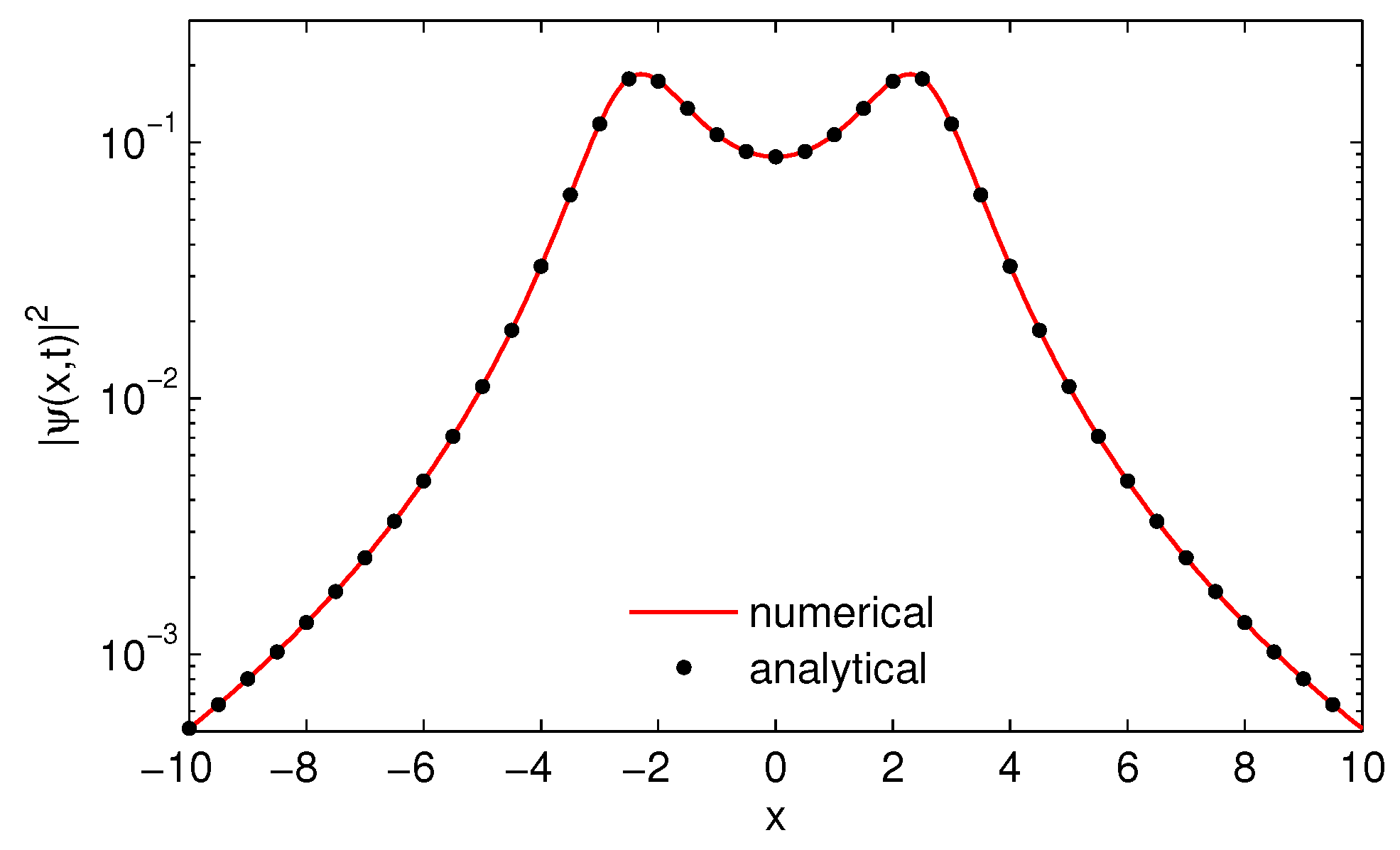
Now, the structure of the matrix M can be readily continued for an arbitrary N. In the following, we use the above described numerical scheme in order to solve the space-fractional Schrödinger Equation (1). We take into account the Cauchy initial wave packet Equation (24) with and evaluate the resulting probability density for and . The size of the computational domain for approximation of the infinite domain is set to . Figure 6 displays the comparison between the analytical solution Equation (31) and the matrix approach Equation (62) for the case of a free particle.
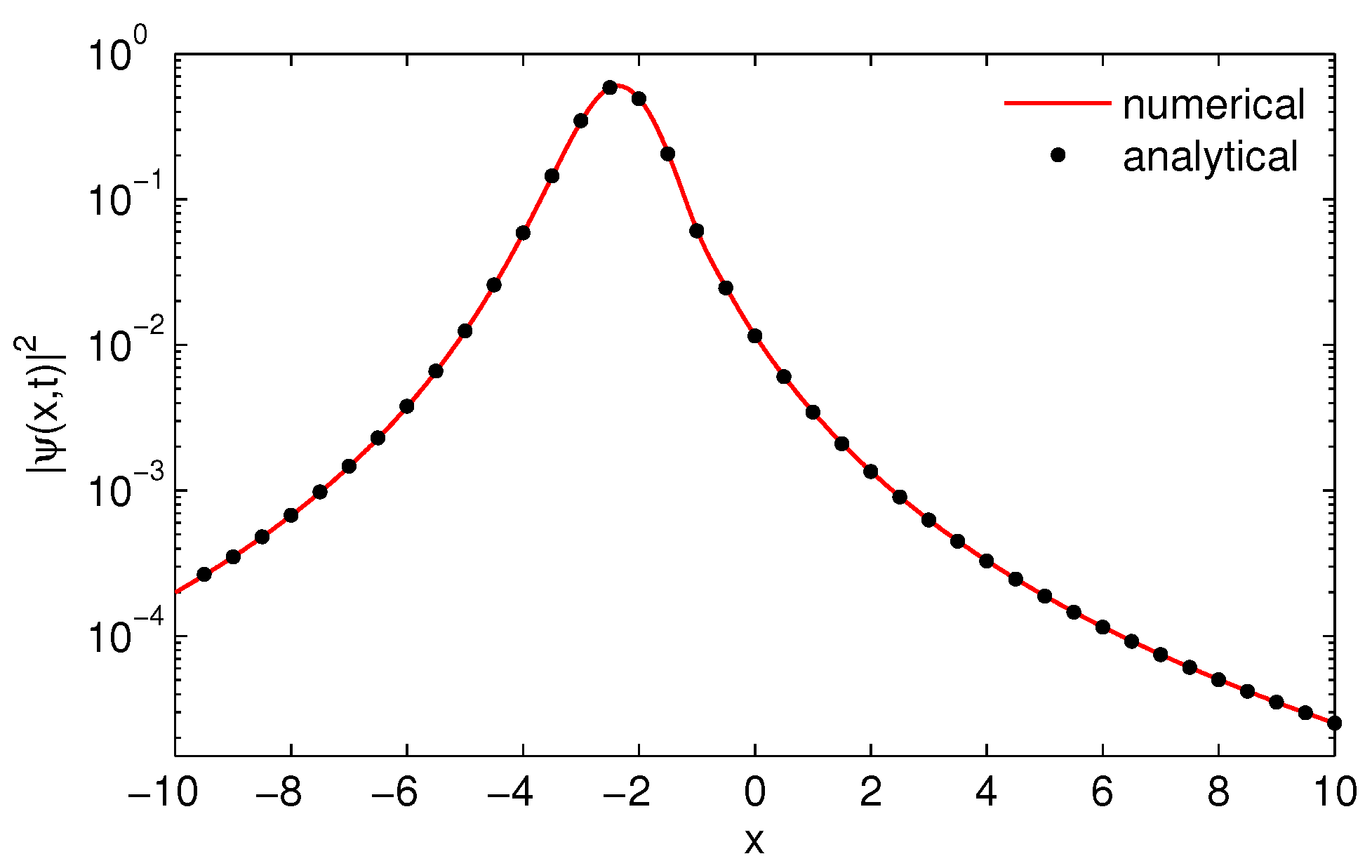
Next, we consider the case of the linear potential with . The resulting probability density belonging to this process is shown in Figure 7. In contrast to the free particle, the probability density is no longer symmetric and additionally exhibits some oscillations.
We repeat the last numerical experiment for the case of a stronger accelerated particle with . The resulting probability density, which is depicted in Figure 8, is given by a smooth curve without oscillations. Furthermore, in contrast to the free particle case, the probability density has not been splitted.
The numerical experiments outlined above confirm both the correctness of the analytical solutions as well as the good quality of the matrix approach. Besides these comparisons, we additionally have performed numerical experiments for other fractional orders α. As a result, we observed in all cases the same good agreement between the analytical solution Equation (10) and the matrix approach Equation (62). It should also be noted that the above matrix approach can be readily extended for solving the space-time fractional Schrödinger equation. More precisely, if we replace the classical time derivative occurring in Equation (1) by the Caputo derivative [24] of order
one obtains the following system of fractional differential equations
The solution to this system is formally given by , where is the Mittag-Leffler matrix function. It can be computed under consideration of the eigenvalue decomposition , where U is a matrix containing the eigenvectors of A. For with eigenvalues , we have together with the diagonal matrix
As a final numerical experiment, we consider the space-time fractional Schrödinger equation
for the joint fractional order . In this case, the wave function in momentum space can be written as , where . The corresponding Green’s function in space domain is available in elementary form as
We note that this result can be derived in a similar manner as the fundamental solution to the neutral-fractional wave equation [25]. The response to an arbitrary initial stage is given by the convolution
In most cases, this integral must be evaluated numerically. However, for the Cauchy initial wave packet Equation (24) the integration can be carried out analytically and summarized as
In Figure 9 we have evaluated the solution of the space-time fractional Schrödinger equation for two different fractional orders subject to the initial stage Equation (20). The analytical solution Equation (69) is denotes by filled dots, whereas the solid line is the numerical solution obtained by means of the Mittag-Leffler matrix function. In both cases the wave function is evaluated for the time value .
5. Conclusions and Discussion
In this article, we considered the space-fractional Schrödinger equation with the Riesz space-fractional derivative in the presence of the linear potential. The general solution to the 1D Schrödinger equation in momentum space has been obtained in closed form, which allows the determination of other measurable quantities such as the spatial moments. Furthermore, we investigated the time evolution of a Cauchy wave packet in detail. Besides the 1D Schrödinger equation we also addressed the case of two spatial dimensions. The obtained equations have been illustrated and verified by comparisons with an independent recently proposed numerical scheme. Consequently, the derived equations are therefore also useful for verification of other numerical approaches which are designed for solving the fractional Schrödinger equation. Besides the space-fractional time-dependent Schrödinger equation solutions to the associated time-independent counterpart are also of importance. Concerning the relationship between the space-fractional time-dependent and time-independent Schrödinger equation we refer to the article [26].
Author Contributions
Both authors have worked together in order to prepare the present manuscript.
Conflicts of Interest
The authors declare no conflict of interest.
References
- Laskin, N. Fractional quantum mechanics. Phys. Rev. E 2000, 62, 3135. [Google Scholar]
- Laskin, N. Fractional Schrödinger equation. Phys. Rev. E 2002, 66, 056108. [Google Scholar] [CrossRef] [PubMed]
- Metzler, R.; Klafter, J. The random walk’s guide to anomalous diffusion: A fractional dynamics approach. Phys. Rep. 2000, 339, 1–77. [Google Scholar] [CrossRef]
- Mainardi, F.; Luchko, Y.; Pagnini, G. The fundamental solution of the space-time fractional diffusion equation. Fract. Calc. Appl. Anal. 2001, 4, 153–192. [Google Scholar]
- Metzler, R.; Klafter, J. The restaurant at the end of the random walk: Recent developments in the description of anomalous transport by fractional dynamics. J. Phys. A Math. Gen. 2004, 37, R161. [Google Scholar] [CrossRef]
- Debnath, L.; Bhatta, D. Integral Transforms and Their Applications; CRC Press: New York, NY, USA, 2014. [Google Scholar]
- Sandev, T.; Metzler, R.; Tomovski, Z. Correlation functions for the fractional generalized Langevin equation in the presence of internal and external noise. J. Math. Phys. 2014, 55, 023301. [Google Scholar] [CrossRef]
- Machida, M. The time-fractional radiative transport equation—Continuous-time random walk, diffusion approximation, and Legendre-polynomial expansion. Available online: http://arxiv.org/abs/1602.05382 (accessed on 25 April 2016).
- Mathai, A.M.; Saxena, R.K.; Haubold, H.J. The H-Function: Theory and Applications; Springer Verlag: New York, NY, USA, 2010. [Google Scholar]
- Zhang, Y.; Liu, X.; Belić, M.R.; Zhong, W.; Zhang, Y.; Xiao, M. Propagation Dynamics of a Light Beam in a Fractional Schrödinger Equation. Phys. Rev. Lett. 2015, 115, 180403. [Google Scholar] [CrossRef] [PubMed]
- Zhang, Y.; Zhong, H.; Belić, M.R.; Ahmed, N.; Zhang, Y.; Xiao, M. Diffraction-free beams in fractional Schrödinger equation. Available online: http://arxiv.org/abs/1512.08671 (accessed on 25 April 2016).
- Zhang, Y.; Zhong, H.; Belić, M.R.; Zhu, Y.; Zhong, W.; Zhang, Y.; Christodoulides, D.N.; Xiao, M. symmetry in a fractional Schrödinger equation. Laser Photonics Rev. 2016. [Google Scholar] [CrossRef]
- Longhi, S. Fractional Schrödinger equation in optics. Opt. Lett. 2015, 40, 1117–1120. [Google Scholar] [CrossRef] [PubMed]
- Robinett, R.W. Quantum mechanical time-development operator for the uniformly accelerated particle. Am. J. Phys. 1996, 64, 803–807. [Google Scholar] [CrossRef]
- Guedes, I. Solution of the Schrödinger equation for the time-dependent linear potential. Phys. Rev. A 2001, 63, 034102. [Google Scholar] [CrossRef]
- Plastino, A.R.; Tsallis, C. Nonlinear Schroedinger equation in the presence of uniform acceleration. J. Math. Phys. 2013, 54, 041505. [Google Scholar] [CrossRef]
- Sandev, T.; Petreska, I.; Lenzi, E.K. Time-dependent Schrödinger-like equation with nonlocal term. J. Math. Phys. 2014, 55, 092105. [Google Scholar] [CrossRef]
- Luchko, Y. Fractional Schrödinger equation for a particle moving in a potential well. J. Math. Phys. 2013, 54, 012111. [Google Scholar] [CrossRef]
- Al-Saqabi, B.; Boyadjiev, L.; Luchko, Y. Comments on employing the Riesz-Feller derivative in the Schrödinger equation. Eur. Phys. J. Spec. Top. 2013, 222, 1779–1794. [Google Scholar] [CrossRef]
- Luchko, Y. Wave-diffusion dualism of the neutral-fractional processes. J. Comput. Phys. 2015, 293, 40–52. [Google Scholar] [CrossRef]
- Adams, D.; Hedberg, L. Function Spaces and Potential Theory; Springer-Verlag: Berlin, Germany, 1999. [Google Scholar]
- Popolizio, M. A matrix approach for partial differential equations with Riesz space fractional derivatives. Eur. Phys. J. Spec. Top. 2013, 222, 1975–1985. [Google Scholar] [CrossRef]
- Dubbeldam, J.L.A.; Tomovski, Z.; Sandev, T. Space-Time Fractional Schrödinger Equation With Composite Time Fractional Derivative. Fract. Calc. Appl. Anal. 2015, 18, 1179–1200. [Google Scholar] [CrossRef]
- Debnath, L. Recent applications of fractional calculus to science and engineering. Int. J. Math. Math. Sci. 2003, 2003, 3413–3442. [Google Scholar] [CrossRef]
- Luchko, Y. Fractional wave equation and damped waves. J. Math. Phys. 2013, 54, 031505. [Google Scholar] [CrossRef]
- Dong, J. Scattering problems in the fractional quantum mechanics governed by the 2D space-fractional Schrödinger equation. J. Math. Phys. 2014, 55, 032102. [Google Scholar] [CrossRef]
Figure 1.
Illustration of the mean square displacement (MSD) Equation (21) for different values of the fractional order α under consideration of the Gaussian initial wave packet Equation (20) with .
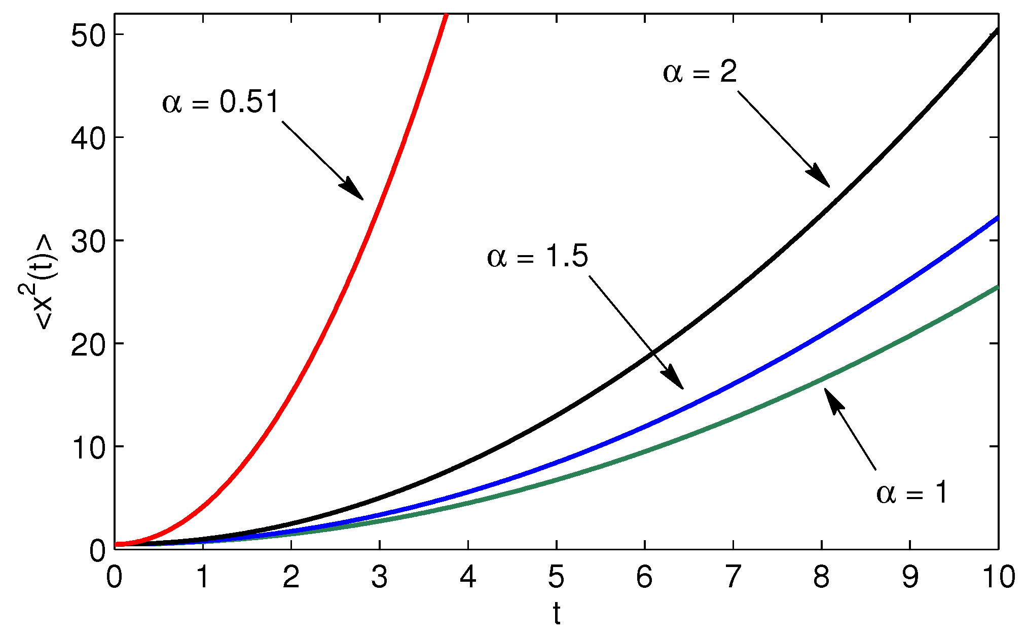
Figure 2.
Time evolution of the Cauchy initial wave packet Equation (24) for the parameter .
Figure 2.
Time evolution of the Cauchy initial wave packet Equation (24) for the parameter .

Figure 3.
Time evolution of the Gaussian initial wave packet Equation (20) for the parameter .
Figure 3.
Time evolution of the Gaussian initial wave packet Equation (20) for the parameter .

Figure 4.
Time evolution of the Cauchy initial wave packet Equation (24) for within the classical quantum mechanics.
Figure 4.
Time evolution of the Cauchy initial wave packet Equation (24) for within the classical quantum mechanics.
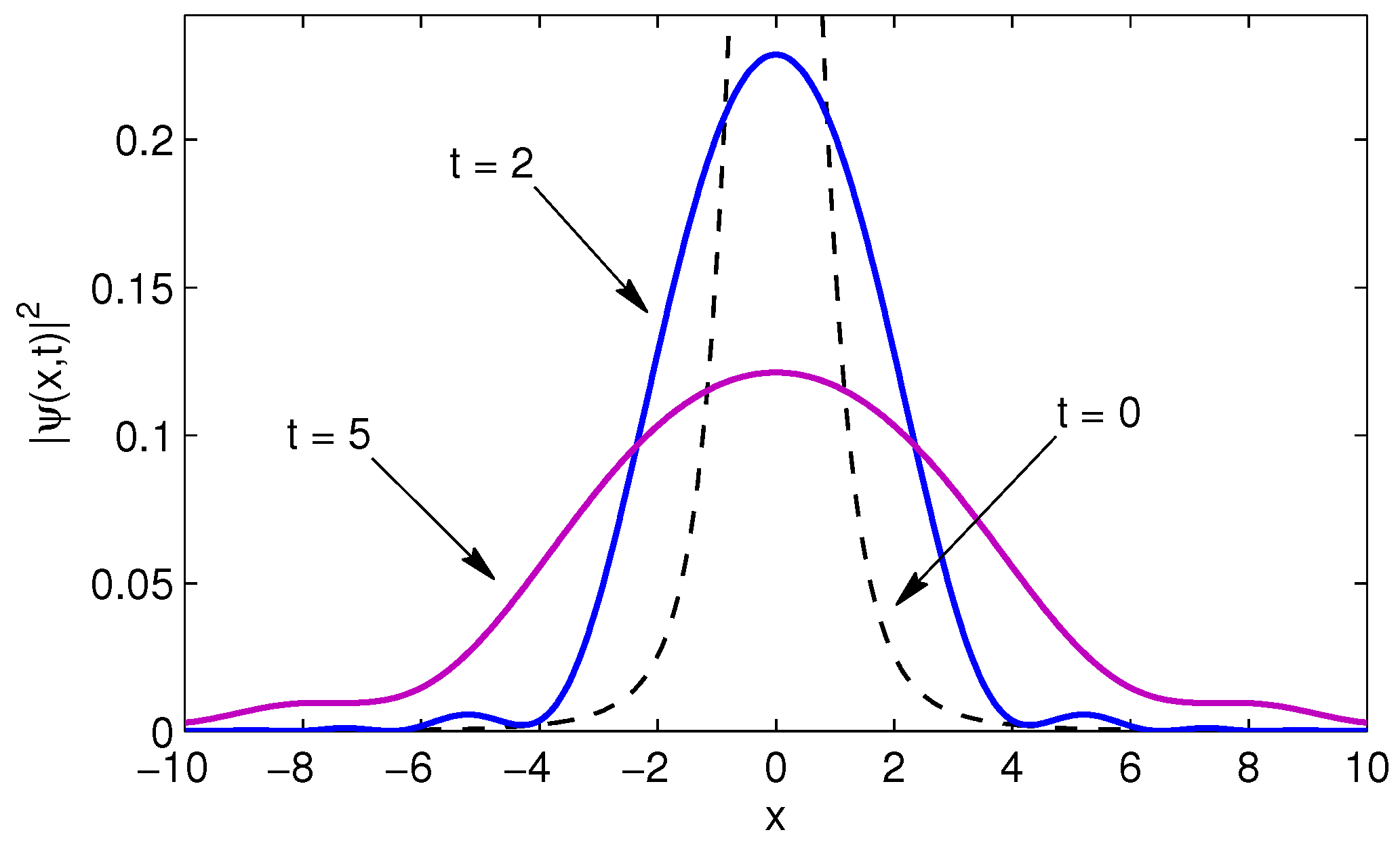
Figure 5.
Time evolution of the rotationally symmetric Cauchy initial wave packet Equation (51) for the parameter .
Figure 5.
Time evolution of the rotationally symmetric Cauchy initial wave packet Equation (51) for the parameter .

Figure 6.
Comparison between the analytical solution Equation (31) and the matrix approach Equation (62) for the case of a free particle.

Figure 7.
Comparison between the analytical solution Equation (25) and the matrix approach Equation (62) for the case of a liner potential with .
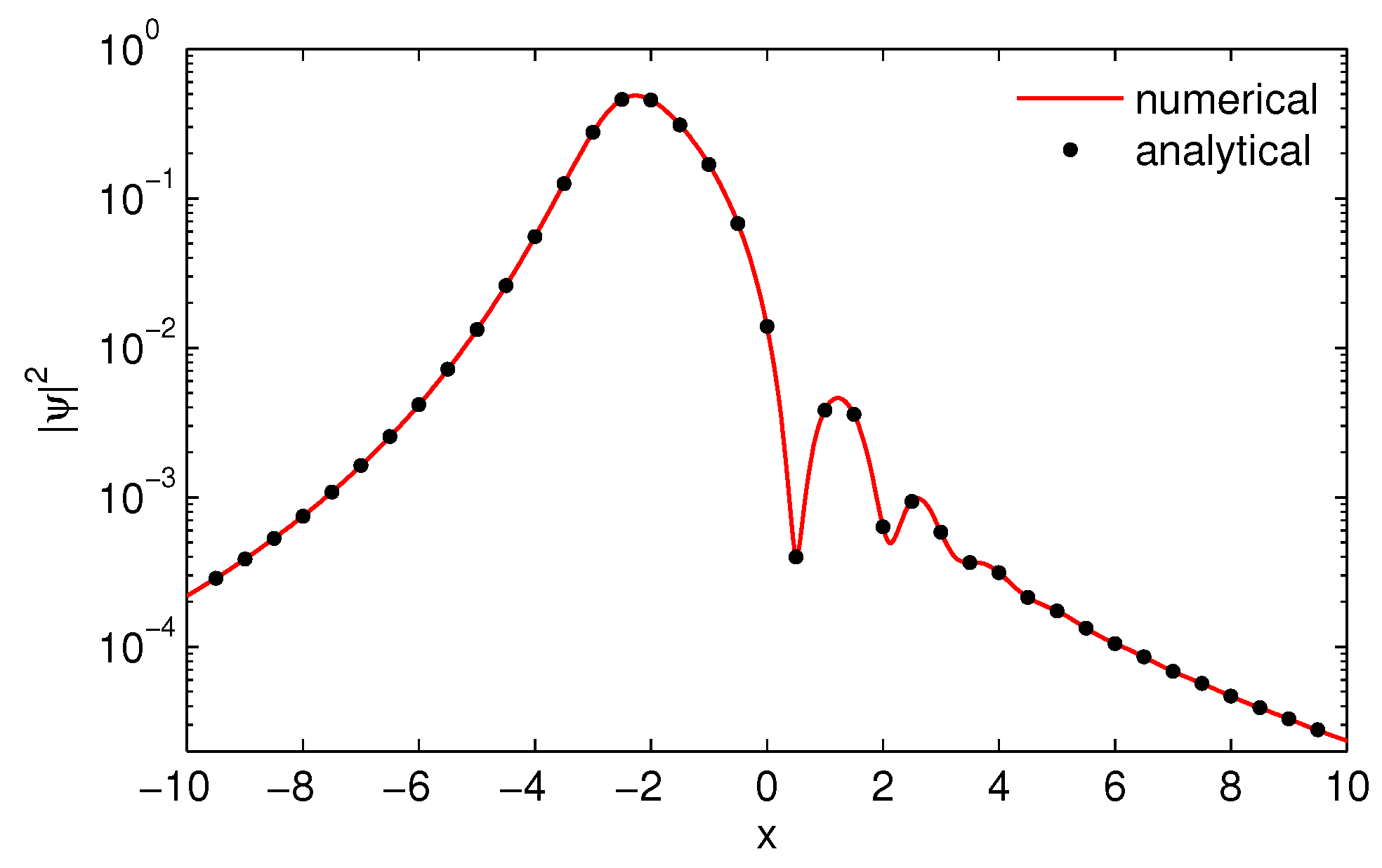
Figure 8.
Comparison between the analytical solution Equation (25) and the matrix approach Equation (62) for the case of a liner potential with .


© 2016 by the authors; licensee MDPI, Basel, Switzerland. This article is an open access article distributed under the terms and conditions of the Creative Commons Attribution (CC-BY) license (http://creativecommons.org/licenses/by/4.0/).
Share and Cite
MDPI and ACS Style
Liemert, A.; Kienle, A. Fractional Schrödinger Equation in the Presence of the Linear Potential. Mathematics 2016, 4, 31. https://doi.org/10.3390/math4020031
AMA Style
Liemert A, Kienle A. Fractional Schrödinger Equation in the Presence of the Linear Potential. Mathematics. 2016; 4(2):31. https://doi.org/10.3390/math4020031
Chicago/Turabian StyleLiemert, André, and Alwin Kienle. 2016. "Fractional Schrödinger Equation in the Presence of the Linear Potential" Mathematics 4, no. 2: 31. https://doi.org/10.3390/math4020031
Note that from the first issue of 2016, this journal uses article numbers instead of page numbers. See further details here.