
Qualitative Properties of Difference Equation of Order Six


1
Department of Mathematics, Faculty of Science, King Abdulaziz University, P.O. Box 80203, Jeddah 21589, Saudi Arabia
2
Department of Mathematics, Faculty of Science, Mansoura University, Mansoura 35516, Egypt
*
Author to whom correspondence should be addressed.
Mathematics 2016, 4(2), 24; https://doi.org/10.3390/math4020024
Submission received: 10 February 2016
/
Revised: 28 March 2016
/
Accepted: 1 April 2016
/
Published: 12 April 2016
Abstract
:In this paper we study the qualitative properties and the periodic nature of the solutions of the difference equation
where the initial conditions are arbitrary positive real numbers and are positive constants. In addition, we derive the form of the solutions of some special cases of this equation.
Mathematics Subject Classification:
39A101. Introduction
This paper deals with behavior of the solutions of the difference equation
where the initial conditions are arbitrary positive real numbers and are constants. In addition, we obtain the form of solution of some special cases.
Recently, there has been great interest in studying difference equation systems. One of the reasons for this is a necessity for some techniques which can be used in investigating equations arising in mathematical models describing real life situations in population biology, economics, probability theory, genetics, psychology, and so forth.
Difference equations appear naturally as discrete analogues and as numerical solutions of differential and delay differential equations having applications in biology, ecology, economy, physics, and so on. Although difference equations are very simple in form, it is extremely difficult to understand thoroughly the behaviors of their solution (see [1,2,3,4,5,6,7,8,9] and the references cited therein). Recently, a great effort has been made in studying the qualitative analysis of rational difference equations and rational difference system (see [10,11,12,13,14,15,16,17,18,19,20,21,22,23]).
Elabbasy et al. [8] studied the boundedness, global stability, periodicity character and gave the solution of some special cases of the difference equation.
Elabbasy and Elsayed [9] investigated the local and global stability, boundedness, and gave the solution of some special cases of the difference equation
In [13], Elsayed investigated the solution of the following non-linear difference equation
Yalçınkaya [26] has studied the following difference equation
For other related work on rational difference equations, see [24,25,26,27,28,29,30,31,32,33,34,35,36,37,38,39,40,41,42,43,44,45,46,47,48,49].
Below, we outline some basic definitions and some theorems that we will need to establish our results.
Let I be some interval of real numbers and let
be a continuously differentiable function. Then for every set of initial conditions , the difference equation
has a unique solution .
A point is called an equilibrium point of Equation (1.2) if
That is, for is a solution of Equation (1.2), or equivalently, is a fixed point of f.
DEFINITION 1.1.
(Equilibrium Point)
A point is called an equilibrium point of Equation (1.2) if
That is, for is a solution of Equation (1.2), or equivalently, is a fixed point of f.
DEFINITION 1.2.
(Periodicity)
A Sequence is said to be periodic with period p if for all
DEFINITION 1.3.
(Fibonacci Sequence)
The sequence
is called Fibonacci Sequence.
DEFINITION 1.4.
(Stability)
- (i)
- The equilibrium point of Equation (1.2) is locally stable if for every there exists such that for all ,withwe have
- (ii)
- The equilibrium point of Equation (1.2) is locally asymptotically stable if is locally stable solution of Equation (1.2) and there exists such that for all , withwe have
- (iii)
- The equilibrium point of Equation (1.2) is global attractor if for all , we have
- (iv)
- The equilibrium point of Equation (1.2) is globally asymptotically stable if is locally stable, and is also a global attractor of Equation (1.2).
- (v)
- The equilibrium point of Equation (1.2) is unstable if is not locally stable.
- (vi)
- The linearized equation of Equation (1.2) about the equilibrium is the linear difference equation
Theorem A.
[38] Assume that and. Then
is a sufficient condition for the asymptotic stability of the difference equation
The following theorem will be useful for establishing the results in this paper.
Theorem B.
[39] Let be an interval of real numbers assume that is a continuous function and consider the following equation
satisfying the following conditions :
- (a)
- is non-decreasing in for each fixed and is non-increasing in for each fixed
- (b)
- For any that is a solution of the systemwe have that
Then Equation (1.4) has a unique equilibrium and every solution of Equation (1.4) converges to
2. Local Stability of the Equilibrium Point of Equation (1.1)
In this section we study the local stability properties of the equilibrium point of Equation (1.1). The equilibrium points of Equation (1.1) are given by the relation
or
If then the unique equilibrium point is
Let be a continuously differentiable function defined by
Therefore
Then the linearized equation of Equation (1.1) about is
Theorem 1.
Assume thatThen the equilibrium point of Equation (1.1) is locally asymptotically stable.
Proof:
From Theorem A, it follows that Equation (2.2) is asymptotically stable if
or
and so
which completes the proof.
3. Global Attractivity of the Equilibrium Point of Equation (1.1)
In this section we investigate the global attractivity character of solutions of Equation (1.1).
Theorem 2.
The equilibrium point of Equation (1.1) is a global attractor if
Proof:
Let are real numbers and assume that be a function defined by Equation (2.1).
Suppose that is a solution of the system
Then from Equation (1.1), we see that
Therefore
or,
thus
From Theorem B, it follows that is a global attractor of Equation (1.1) and then the proof is complete.
4. Boundedness of Solutions of Equation (1.1)
In this section we study the boundedness of solution of Equation (1.1)
Theorem 3.
Every solution of Equation(1.1) is bounded if
Proof:
Let be a solution of Equation (1.1). It follows from Equation (1.1) that
Then
Then the sub-sequences and are decreasing and so are bounded from above by
5. Special Cases of Equation (1.1)
5.1. First Equation
In this section we study the following special case of Equation (1.1)
where the initial conditions are arbitrary real numbers.
Theorem 4.
Letbe a solution of Equation (5.1) then for
where
Proof:
We prove that the forms given are solutions of Equation (5.1) by using mathematical induction. First, we let then the result holds. Second, we assume that the expressions are satisfied for . Our objective is to show that the expressions are satisfied for n. That is;
Now, it follows from Equation (5.1) that,
Therefore
Also, we see from Equation (5.1) that,
Then
Also, wee see from Equation (5.1) that,
Thus
Hence, the proof is complete.
We will confirm our result by considering some numerical examples assume (See Figure 3).
5.2. Second Equation
In this section we solve a more specific form of Equation (1.1)
where the initial conditions are arbitrary real numbers.
Theorem 5.
Letbe a solution of Equation (5.3). Then for
where
Proof:
The proof is the same as for Theorem 4 and is therefore omitted.
To confirm our result assume (See Figure 4).
5.3. Third Equation
In this section we deal with the following special case of Equation (1.1)
where the initial conditions are arbitrary real numbers.
Theorem 6.
Let be a solution of Equation(5.5) then for
where
Proof:
For , the result holds. Now suppose that and that our assumption holds for That is,
Now, it follows from Equation (5.3) that,
Also, from Equation (5.3), we see that,
Also, from Equation (5.3), we get,
Hence, the proof is complete.
We consider a numerical example of this special case, assume (See Figure 5).
5.4. Fourth Equation
In this section we deal with the form of solution of the following equation
where the initial conditions are arbitrary real numbers.
Theorem 7.
Let be a solution of Equation (5.4) Then every solution of Equation (5.4) is periodic with period 18. Moreover, takes the form
or,
where
Proof:
The proof is the same as the proof of Theorem 6 and thus will be omitted.
Figure 6 shows the solution when
6. Conclusions
In this paper we investigated the global attractivity, boundedness and the solutions of some special cases of Equation (1.1). In Section 2 we proved when , Equation (1.1) has local stability. In Section 3 we showed that the unique equilibrium of Equation (1.1) is globally asymptotically stable if In Section 4 we investigated that the solution of Equation (1.1) is bounded if . In Section 5 we obtained the form of the solution of four special cases of Equation (1.1) and gave numerical examples of each of the case with different initial values.
Acknowledgments
The authors thank the main editor and anonymous referees for their valuable suggestions and comments leading to improvement of this paper.
Author Contributions
All authors carried out the proofs of the main results and approved the final manuscript.
Conflicts of Interest
The authors declare no conflict of interest.
References
- Ahmed, A.M.; Youssef, A.M. A solution form of a class of higher-order rational difference equations. J. Egyp. Math. Soc. 2013, 21, 248–253. [Google Scholar] [CrossRef]
- Alghamdi, M.; Elsayed, E.M.; El-Dessoky, M.M. On the Solutions of Some Systems of Second Order Rational Difference Equations. Life Sci. J. 2013, 10, 344–351. [Google Scholar]
- Asiri, A.; Elsayed, E.M.; El-Dessoky, M.M. On the Solutions and Periodic Nature of Some Systems of Difference Equations. J. Comput. Theor. Nanosci. 2015, 12, 3697–3704. [Google Scholar] [CrossRef]
- Das, S.E.; Bayram, M. On a System of Rational Difference Equations. World Appl. Sci. J. 2010, 10, 1306–1312. [Google Scholar]
- Din, Q. Qualitative nature of a discrete predator-prey system. Contemp. Methods Math. Phys. Gravit. 2015, 1, 27–42. [Google Scholar]
- Din, Q. Stability analysis of a biological network. Netw. Biol. 2014, 4, 123–129. [Google Scholar]
- Din, Q.; Elsayed, E.M. Stability analysis of a discrete ecological model. Comput. Ecol. Softw. 2014, 4, 89–103. [Google Scholar]
- Elabbasy, E.M.; El-Metwally, H.; Elsayed, E.M. On the Difference Equation . Acta Math. Vietnam. 2008, 33, 85–94. [Google Scholar]
- Elabbasy, E.M.; Elsayed, E.M. Dynamics of a rational difference equation. Chin. Ann. Math. Ser. B 2009, 30, 187–198. [Google Scholar] [CrossRef]
- El-Dessoky, M.M.; Elsayed, E.M. On the solutions and periodic nature of some systems of rational difference equations. J. Comput. Anal. Appl. 2015, 18, 206–218. [Google Scholar]
- El-Metwally, H.; Elsayed, E.M. Qualitative Behavior of some Rational Difference Equations. J. Comput. Anal. Appl. 2016, 20, 226–236. [Google Scholar]
- El-Moneam, M.A. On the dynamics of the solutions of the rational recursive sequences. Br. J. Math. Comput. Sci. 2015, 5, 654–665. [Google Scholar] [CrossRef] [PubMed]
- Elsayed, E.M. Qualitative behaviour of difference equation of order two. Math. Comput. Model. 2009, 50, 1130–1141. [Google Scholar] [CrossRef]
- Elsayed, E.M. Solution and attractivity for a rational recursive sequence. Discret. Dyn. Nat. Soc. 2011, 2011, 982309. [Google Scholar] [CrossRef]
- Elsayed, E.M. Solutions of rational difference system of order two. Math. Comput. Mod. 2012, 55, 378–384. [Google Scholar] [CrossRef]
- Elsayed, E.M. Behavior and expression of the solutions of some rational difference equations. J. Comput. Anal. Appl. 2013, 15, 73–81. [Google Scholar]
- Elsayed, E.M. Solution for systems of difference equations of rational form of order two. Comput. Appl. Math. 2014, 33, 751–765. [Google Scholar] [CrossRef]
- Elsayed, E.M. On the solutions and periodic nature of some systems of difference equations. Int. J. Biomath. 2014, 7, 1450067. [Google Scholar] [CrossRef]
- Elsayed, E.M. New method to obtain periodic solutions of period two and three of a rational difference equation. Nonlinear Dyn. 2015, 79, 241–250. [Google Scholar] [CrossRef]
- Elsayed, E.M. Dynamics and Behavior of a Higher Order Rational Difference Equation. J. Nonlinear Sci. Appl. 2016, 9, 1463–1474. [Google Scholar]
- Elsayed, E.M.; Ahmed, A.M. Dynamics of a three-dimensional systems of rational difference equations. Math. Methods Appl. Sci. 2016, 39, 1026–1038. [Google Scholar] [CrossRef]
- Elsayed, E.M.; Alghamdi, A. Dynamics and Global Stability of Higher Order Nonlinear Difference Equation. J. Comput. Anal. Appl. 2016, 21, 493–503. [Google Scholar]
- Elsayed, E.M.; El-Dessoky, M.M. Dynamics and global behavior for a fourth-order rational difference equation. Hacet. J. Math. Stat. 2013, 42, 479–494. [Google Scholar]
- Karatas, R.; Cinar, C.; Simsek, D. On positive solutions of the difference equation . Int. J. Contemp. Math. Sci. 2006, 1, 495–500. [Google Scholar]
- Saleh, M.; Aloqeili, M. On the difference equation Appl. Math. Comput. 2006, 176, 359–363. [Google Scholar] [CrossRef]
- Yalçınkaya, I. On the difference equation . Discret. Dyn. Nat. Soc. 2008, 2008, 805460. [Google Scholar] [CrossRef]
- Elsayed, E.M.; El-Dessoky, M.M.; Alzahrani, E.O. The Form of The Solution and Dynamics of a Rational Recursive Sequence. J. Comput. Anal. Appl. 2014, 17, 172–186. [Google Scholar]
- Elsayed, E.M.; El-Dessoky, M.M.; Asiri, A. Dynamics and Behavior of a Second Order Rational Difference equation. J. Comput. Anal. Appl. 2014, 16, 794–807. [Google Scholar]
- Elsayed, E.M.; El-Metwally, H. Stability and solutions for rational recursive sequence of order three. J. Comput. Anal. Appl. 2014, 17, 305–315. [Google Scholar]
- Elsayed, E.M.; El-Metwally, H. Global behavior and periodicity of some difference equations. J. Comput. Anal. Appl. 2015, 19, 298–309. [Google Scholar]
- Elsayed, E.M.; Ibrahim, T. F. Solutions and periodicity of a rational recursive sequences of order five. Bull. Malays. Math. Sci. Soc. 2015, 38, 95–112. [Google Scholar] [CrossRef]
- Elsayed, E.M.; Ibrahim, T.F. Periodicity and solutions for some systems of nonlinear rational difference equations. Hacet. J. Math. Stat. 2015, 44, 1361–1390. [Google Scholar] [CrossRef]
- Halim, Y.; Bayram, M. On the solutions of a higher-order difference equation in terms of generalized Fibonacci sequences. Math. Methods Appl. Sci. 2015. [Google Scholar] [CrossRef]
- Ibrahim, T.F.; Touafek, N. Max-type system of difference equations with positive two-periodic sequences. Math. Methods Appl. Sci. 2014, 37, 2562–2569. [Google Scholar] [CrossRef]
- Ibrahim, T.F.; Touafek, N. On a third order rational difference equation with variable coefficients. Dyn. Contol Disc Imput Syst. Appl. Algo. 2013, 20, 251–264. [Google Scholar]
- Jana, D.; Elsayed, E.M. Interplay between strong Allee effect, harvesting and hydra effect of a single population discrete-time system. Int. J. Biomath. 2016, 9, 1650004. [Google Scholar] [CrossRef]
- Khaliq, A.; Elsayed, E.M. The Dynamics and Solution of some Difference Equations. J. Nonlinear Sci. Appl. 2016, 9, 1052–1063. [Google Scholar]
- Khan, A.Q.; Qureshi, M.N. Global dynamics of a competitive system of rational difference equations. Math. Methods Appl. Sci. 2015, 38, 4786–4796. [Google Scholar] [CrossRef]
- Khan, A.Q.; Qureshi, M.N.; Din, Q. Asymptotic behavior of an anti-competitive system of rational difference equations. Life Sci. J. 2014, 11, 16–20. [Google Scholar]
- Kocic, V.L.; Ladas, G. Global Behavior of Nonlinear Difference Equations of Higher Order with Applications; Kluwer Academic Publishers: Dordrecht, The Netherlands, 1993. [Google Scholar]
- Kulenovic, M.R.S.; Ladas, G. Dynamics of Second Order Rational Difference Equations with Open Problems and Conjectures; Chapman & Hall / CRC Press: London, UK, 2001. [Google Scholar]
- Kurbanli, A.S. On the Behavior of Solutions of the System of Rational Difference Equations. World Appl. Sci. J. 2010, 10, 1344–1350. [Google Scholar]
- Simsek, D.; Cinar, C.; Yalcinkaya, I. On the recursive sequence Int. J. Contemp. Math. Sci. 2006, 1, 475–480. [Google Scholar]
- Touafek, N. On a second order rational difference equation. Hacet. J. Math. Stat. 2012, 41, 867–874. [Google Scholar]
- Yalcinkaya, I.; Cinar, C. On the dynamics of difference equation . Fasc. Math. 2009, 42, 141–148. [Google Scholar]
- Yazlik, Y.; Elsayed, E.M.; Taskara, N. On the Behaviour of the Solutions of Difference Equation Systems. J. Comput. Anal. Appl. 2014, 16, 932–941. [Google Scholar]
- Yazlik, Y.; Tollu, D.T.; Taskara, N. On the solutions of a max-type difference equation system. Math. Methods Appl. Sci. 2015, 38, 4388–4410. [Google Scholar] [CrossRef]
- Zayed, E.M.E.; El-Moneam, M.A. On the rational recursive sequence Commun. Appl. Nonlinear Anal. 2005, 12, 15–28. [Google Scholar]
- Zayed, E.M.E.; El-Moneam, M.A. On the rational recursive sequence . Commun. Appl. Nonlinear Anal. 2008, 15, 47–57. [Google Scholar]
Figure 1.
Expresses the solution of , when we put initials and constants
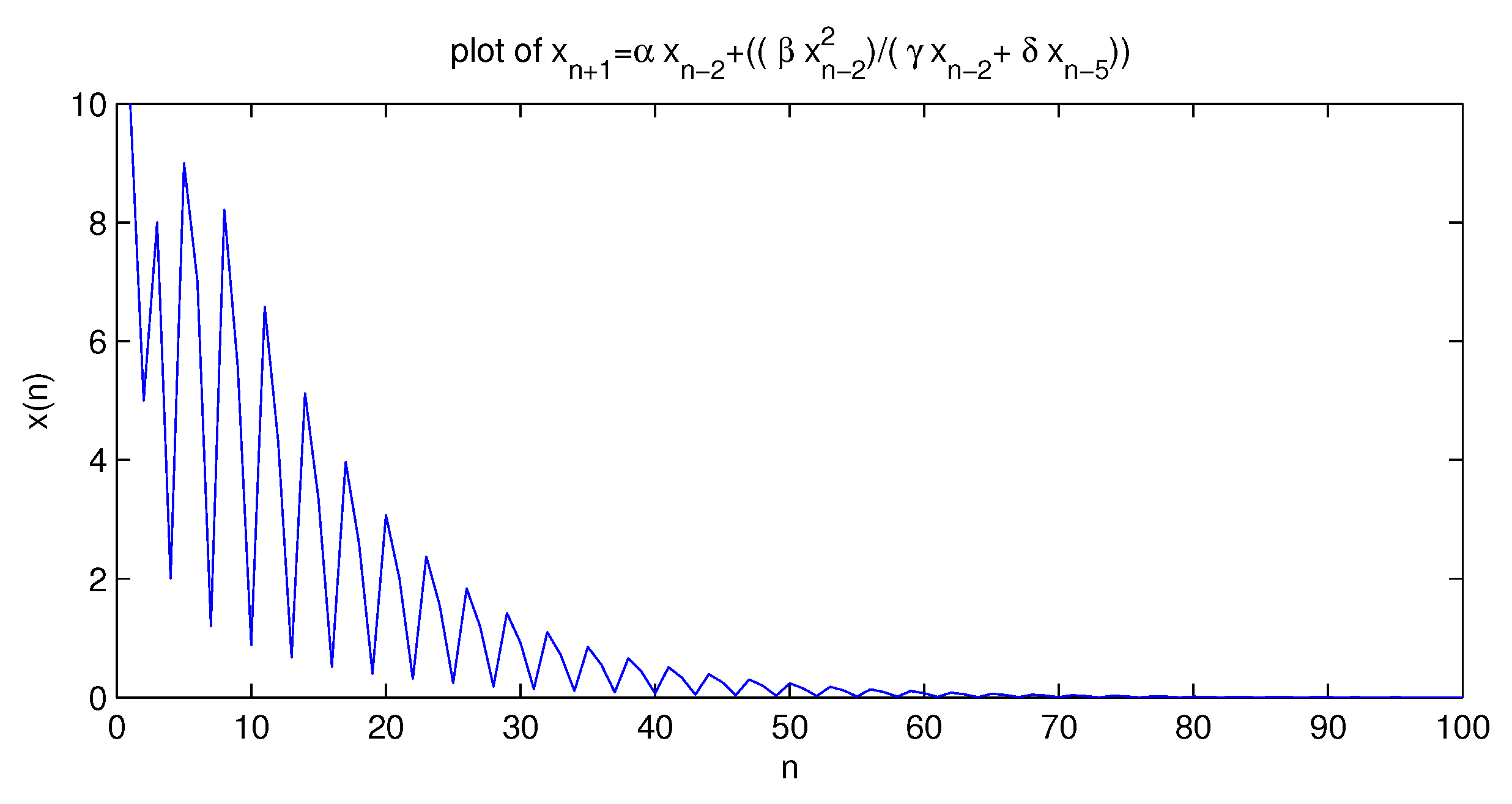
Figure 2.
Represents behavior of Equation (1.1) when
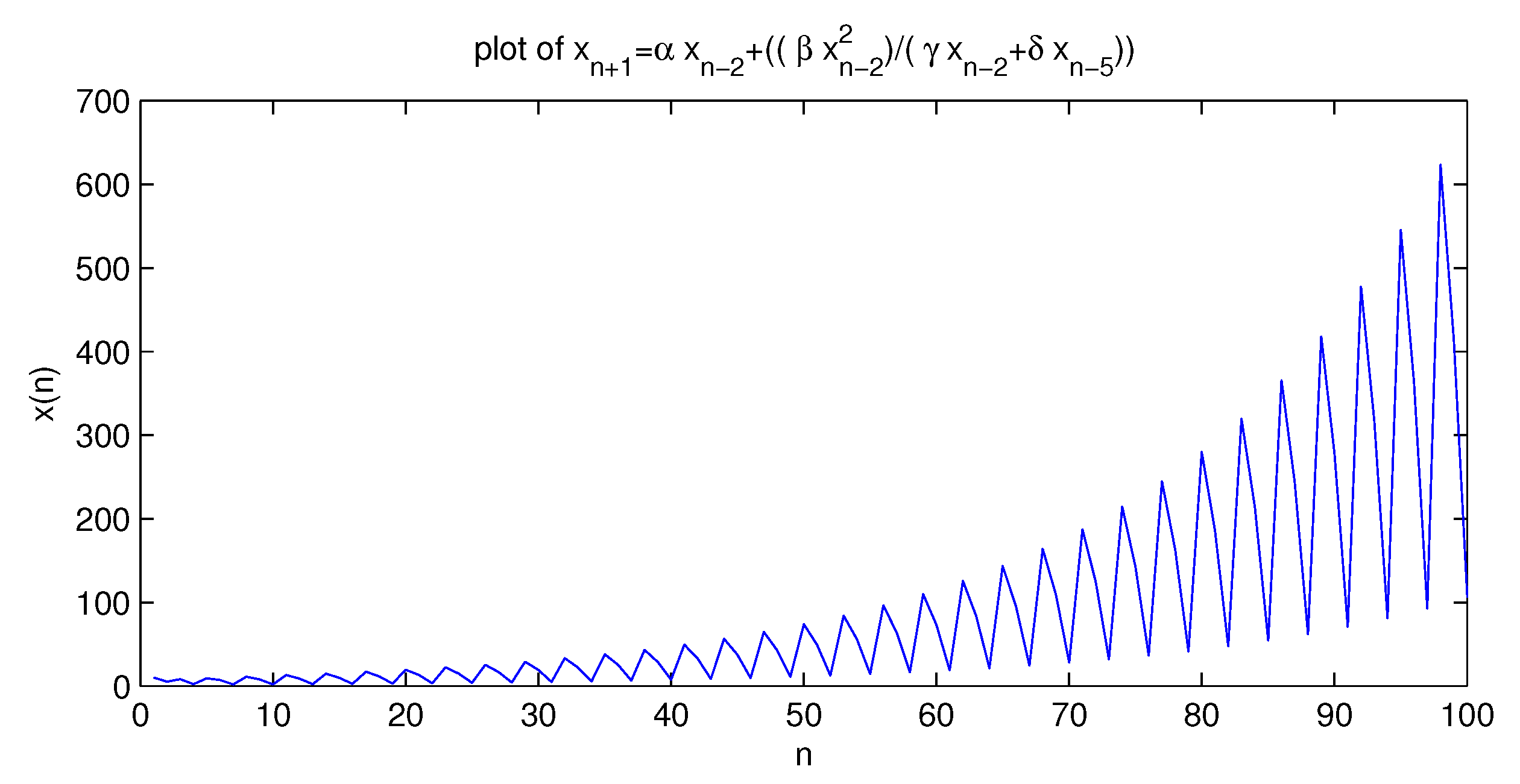
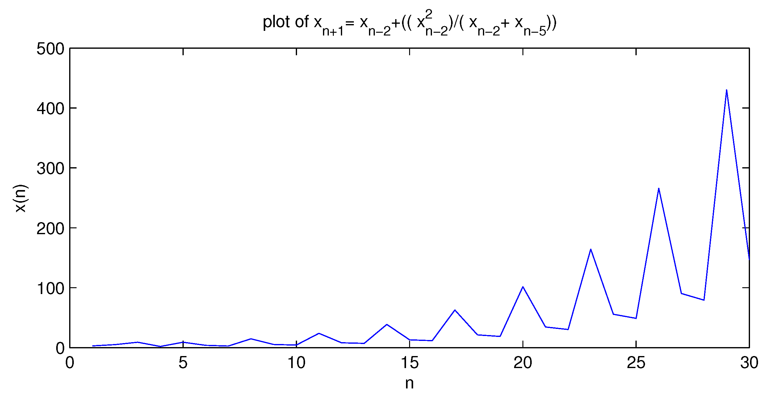
Figure 3.
Shows the behavior for Equation (5.1) with

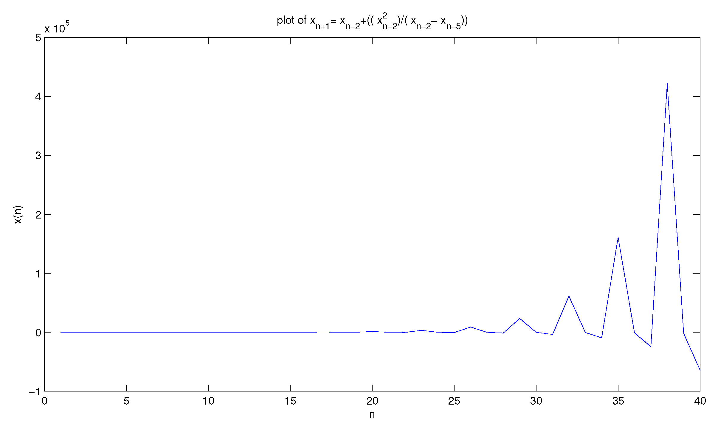
Figure 4.
Shows solution of Equation (5.2) with

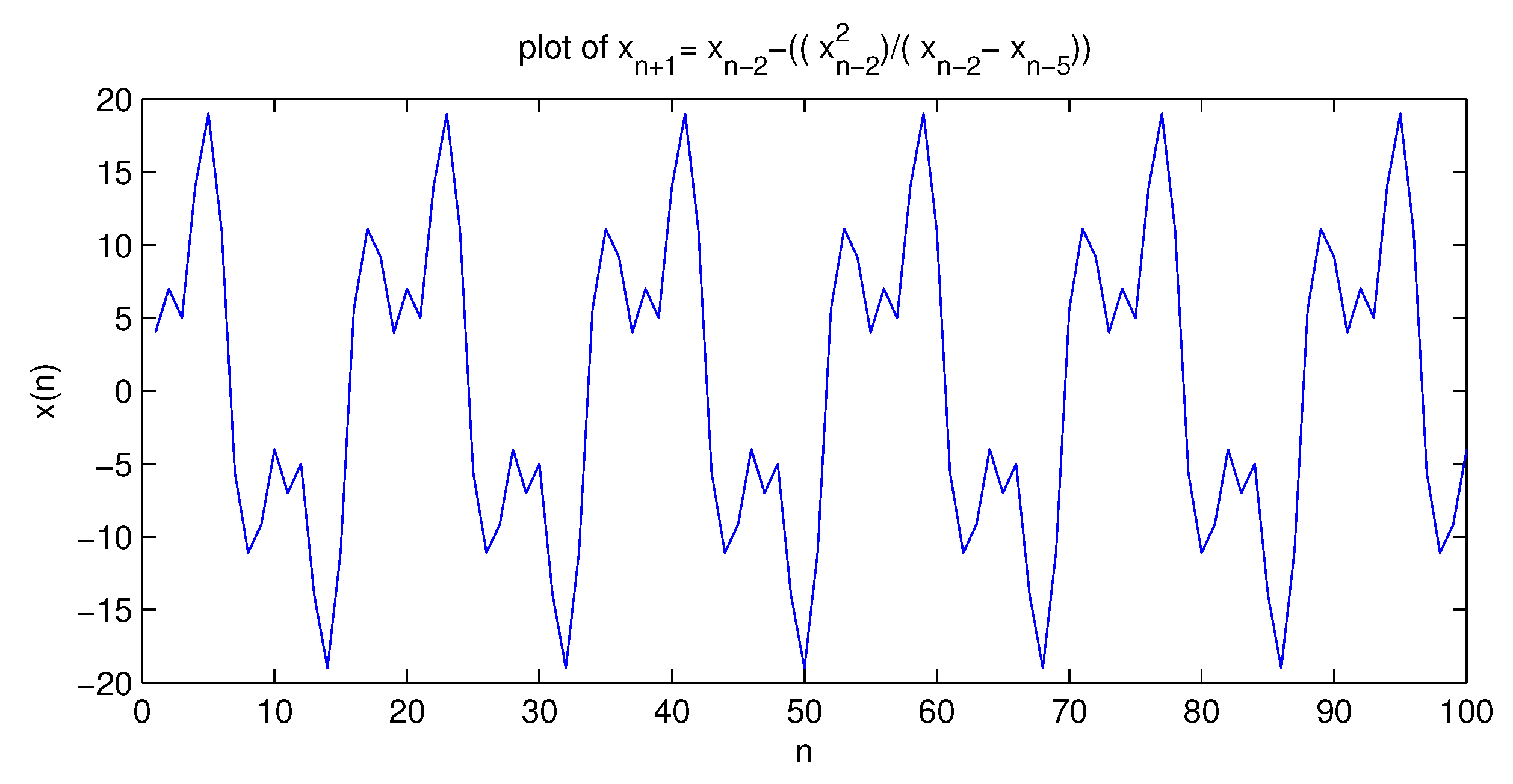
Figure 5.
Shows the dynamics of Equation (5.3) when
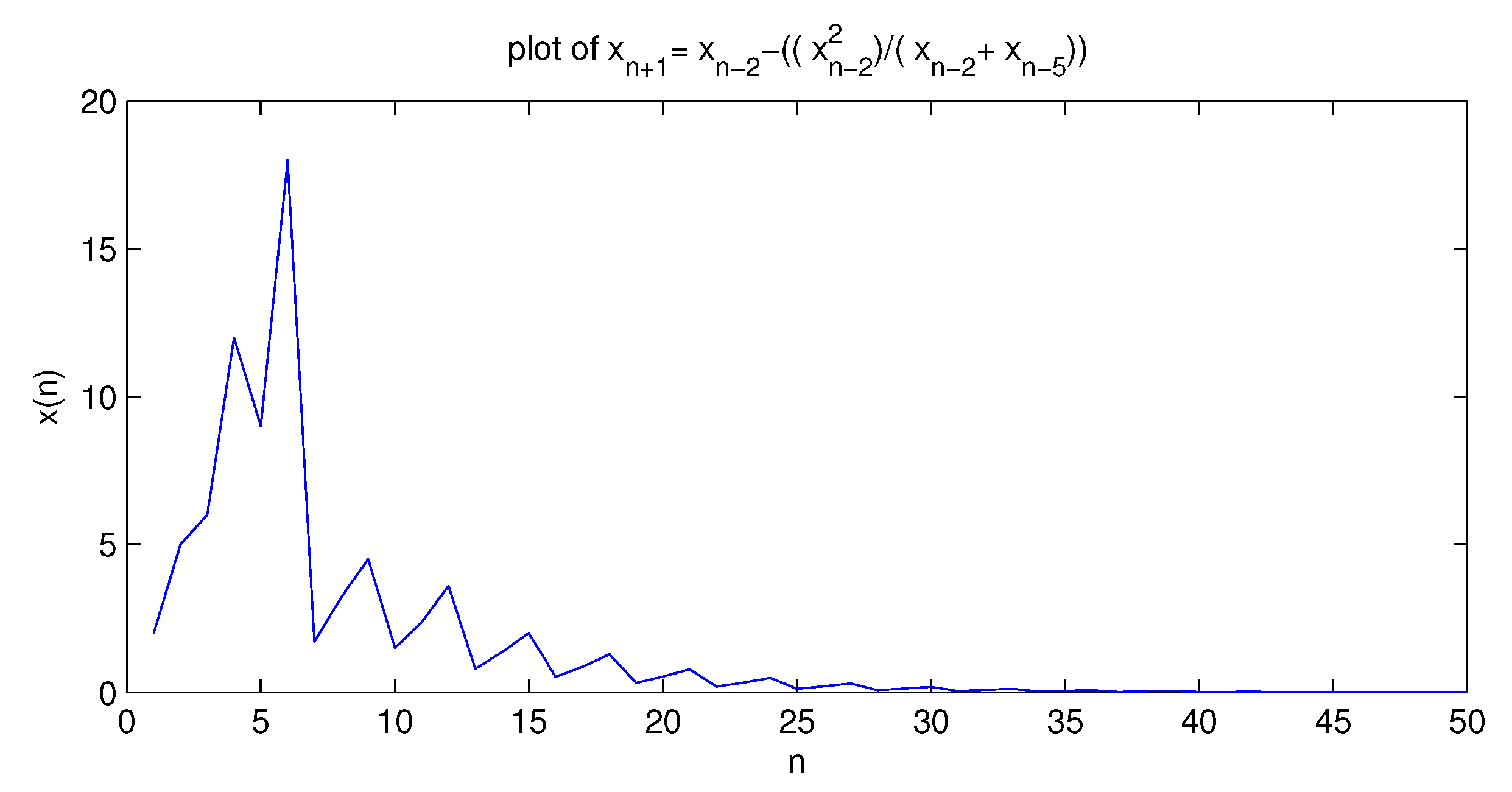
Figure 6.
Shows the periodic behavior of solution of , with

© 2016 by the authors; licensee MDPI, Basel, Switzerland. This article is an open access article distributed under the terms and conditions of the Creative Commons by Attribution (CC-BY) license (http://creativecommons.org/licenses/by/4.0/).
Share and Cite
MDPI and ACS Style
Khaliq, A.; Elsayed, E.M. Qualitative Properties of Difference Equation of Order Six. Mathematics 2016, 4, 24. https://doi.org/10.3390/math4020024
AMA Style
Khaliq A, Elsayed EM. Qualitative Properties of Difference Equation of Order Six. Mathematics. 2016; 4(2):24. https://doi.org/10.3390/math4020024
Chicago/Turabian StyleKhaliq, Abdul, and E.M. Elsayed. 2016. "Qualitative Properties of Difference Equation of Order Six" Mathematics 4, no. 2: 24. https://doi.org/10.3390/math4020024
Note that from the first issue of 2016, this journal uses article numbers instead of page numbers. See further details here.