Optimal Intervention Strategies for a SEIR Control Model of Ebola Epidemics

Abstract

A SEIR control model describing the Ebola epidemic in a population of a constant size is considered over a given time interval. It contains two intervention control functions reflecting efforts to protect susceptible individuals from infected and exposed individuals. For this model, the problem of minimizing the weighted sum of total fractions of infected and exposed individuals and total costs of intervention control constraints at a given time interval is stated. For the analysis of the corresponding optimal controls, the Pontryagin maximum principle is used. According to it, these controls are bang-bang, and are determined using the same switching function. A linear non-autonomous system of differential equations, to which this function satisfies together with its corresponding auxiliary functions, is found. In order to estimate the number of zeroes of the switching function, the matrix of the linear non-autonomous system is transformed to an upper triangular form on the entire time interval and the generalized Rolle’s theorem is applied to the converted system of differential equations. It is found that the optimal controls of the original problem have at most two switchings. This fact allows the reduction of the original complex optimal control problem to the solution of a much simpler problem of conditional minimization of a function of two variables. Results of the numerical solution to this problem and their detailed analysis are provided.

1. Introduction

Ebola is a lethal virus for humans. It was previously confined to Central Africa, but recently was also identified in West Africa ([1]). As of October 8, 2014, the World Health Organization (WHO) reported 4656 cases of Ebola virus deaths, with most cases occurring in Liberia ([2]). The extremely rapid increase of the disease, high mortality rate, and the nonexistence of a vaccine make this virus a major problem for public health. Ebola is transmitted through direct contact with blood, bodily secretions and tissues of infected humans and primates ([3,4]). Therefore, the practical control interventions of public health measures are major factors for stopping Ebola transmission. To understand the dynamics of the spread of Ebola infection in the affected countries, it is crucial to have models of this process to simulate.

In this paper we focus our attention on a SEIR deterministic model and its use for the description of the Ebola epidemics ([5,6,7]). In order to deal with the epidemics of Ebola, governments of affected countries decided to implement intervention measures: some applied social distancing, early detection of infectious individuals, quarantine procedures, campaigns for information and education, and acceleration of the burial process. In this context, we introduce into the SEIR model the control functions reflecting these intervention measures and consider the optimal control problem to study the effect of these intervention control strategies on the epidemic spread. Optimality is measured as the minimization of the weighted sum of total fractions of infected end exposed individuals and the total cost of intervention control constraints over a given time interval.

We model the effects from intervention control measures by reducing the rate at which the disease is contracted from an average individual during such measures (called shortly transmission rate). We justify this as follows: suppose during an outbreak one starts the measures orienting susceptible individuals to avoid contracting the virus (assuming some protective behavior, for example, washing hands, avoiding close environments, etc.). The effect of these measures will be that the probability of a susceptible individual contracting the virus will decrease. This reduction (increase) is bounded below (above) and costs of such measures are linear on the controls. Hence, the original problem renders itself to analytical treatment and we can establish the main properties about optimal strategies of intervention control measures. It simplifies the problem and allows its complete numerical study. Influence of health-promotion and educational campaigns on the spread of epidemic, which is described by various SIR models, was previously studied in [8,9].

The paper is organized as follows. In Section 2, we introduce a SEIR control model, describe its variables, control functions, parameters and study the properties of these variables. In Section 3 we state the optimal control problem and consider in detail the epidemiological significance of the introduced functional. Next, we discuss the existence of the optimal solutions in our problem. In Section 4, for the analysis of these solutions, we use the Pontryagin maximum principle to write the Hamiltonian of the optimal control problem and corresponding adjoint system and find the formulas which determine the appropriate optimal controls through solutions of this system. Based on these formulas we find the switching function that defines the type of the optimal controls. Finally, we obtain the system of differential equations to which this function satisfies with its corresponding auxiliary functions. Section 5 is devoted to studying the properties of the switching function, which lead to the conclusion regarding bang-bang type of the optimal controls and help in the estimation of the number of switchings. These results are the basis of the method of the solution to the optimal control problem, a description of which is given in Section 6. Here the Lipschitz constant is found for use in the numerical algorithm. Results of numerical calculations and their detailed analysis are presented in Section 7. Finally, Section 8 contains our conclusions.

2. SEIR Model and Its Properties

At a given time interval $[0,T]$ we consider a SEIR model described by the following system of differential equations:

$$\left\{\begin{array}{c}\dot{S}\left(t\right)=-N^{-1}\left(\beta I\left(t\right)+\alpha E\left(t\right)\right)S\left(t\right),\hfill \\ \dot{E}\left(t\right)=N^{-1}\left(\beta I\left(t\right)+\alpha E\left(t\right)\right)S\left(t\right)-\delta E\left(t\right),\hfill \\ \dot{I}\left(t\right)=\delta E\left(t\right)-\gamma I\left(t\right),\hfill \\ \dot{R}\left(t\right)=\gamma I\left(t\right),\hfill \\ S\left(0\right)=S_0,E\left(0\right)=E_0,I\left(0\right)=I_0,R\left(0\right)=R_0;S_0,E_0,I_0,R_0>0.\hfill \end{array}\right.$$

(1)

Such a model describes the spread of the epidemic in a population of the constant size N. Indeed, considering that the equality

$$S_0+E_0+I_0+R_0=N$$

(2)

holds, we add together the equations of system (1). Taking into account relationship (2), we find the equality:

$$S\left(t\right)+E\left(t\right)+I\left(t\right)+R\left(t\right)=N.$$

(3)

System (1) was used in [5] to describe the Ebola outbreak in Zaire (1976), then, in [6], for studying the effects of public health measures during Ebola outbreaks in Congo (1995) and Uganda (2000). Finally, this system was applied in [7] for the study of recent Ebola outbreaks in Guinea, Liberia and Sierra Leone (2014).

In system (1) the quantity $S\left(t\right)$ is the number of susceptible individuals. The quantity $E\left(t\right)$ denotes the number of individuals exposed to the virus of infected but not yet infectious. Individuals that are infected with the disease and are suffering the symptoms of Ebola are classified as infectious individuals, the number of them is denoted by $I\left(t\right)$. Similarly, the number of deceased or recovered individuals is denoted by $R\left(t\right)$. In system (1) the value $\beta N^{-1}I\left(t\right)S\left(t\right)$ is the number of individuals infected due to direct contact with an infected individual, and the value $\alpha N^{-1}E\left(t\right)S\left(t\right)$ is the number of individuals infected due to direct contact with an exposed individual. Here β is the transmission rate; $\alpha =q\beta$, where $q\in [0,1]$ is a weight factor taking into account that a susceptible individual has a higher chance of getting infected from an infectious individual than from an exposed individual. The value $\delta E\left(t\right)$ is the individuals in the exposed stage, which show symptoms of the disease and pass on to the infectious stage; δ is the infectious rate. The value $\gamma I\left(t\right)$ is the individuals in the infectious stage, which die; γ is the death rate. We consider that death and recovery are taken to be the same, since there has not been a case in which a person who survived Ebola contracts the disease again.

Now, we will make controllable SEIR model, described by system (1). For this, we introduce two control functions $u\left(t\right)$, $v\left(t\right)$ implying the efforts of preventing susceptible individuals from becoming infectious individuals as a result of contact with infectious and exposed ones. For our controls we have the following constraints:

$$0<u_{min}\le u\left(t\right)\le u_{max},0\le v_{min}\le v\left(t\right)\le v_{max},$$

(4)

where $u_{max}=\beta$, $v_{max}=\alpha$. We observe that the control functions $u\left(t\right)$, $v\left(t\right)$ regulate the goals and efforts of two similar interventions. In the case of control $u\left(t\right)$, the equality $u\left(t\right)=\beta$ corresponds to not having an intervention affecting the susceptible individuals and the equality $u\left(t\right)=u_{min}$ corresponds to the maximum effort that can be made. Similar conclusions are valid for the control $v\left(t\right)$. Today there are no licensed treatment and approved vaccines for Ebola; there are examples of experimental vaccines as proof of the possibility of treatment by vaccinating infected individuals (see [10]). Therefore, controlled interventions are the major factor for stopping Ebola transmission.

Thus, we have the following SEIR control model of the type:

$$\left\{\begin{array}{c}\dot{S}\left(t\right)=-N^{-1}\left(u\left(t\right)I\left(t\right)+v\left(t\right)E\left(t\right)\right)S\left(t\right),t\in [0,T],\hfill \\ \dot{E}\left(t\right)=N^{-1}\left(u\left(t\right)I\left(t\right)+v\left(t\right)E\left(t\right)\right)S\left(t\right)-\delta E\left(t\right),\hfill \\ \dot{I}\left(t\right)=\delta E\left(t\right)-\gamma I\left(t\right),\hfill \\ S\left(0\right)=S_0,E\left(0\right)=E_0,I\left(0\right)=I_0,\hfill \\ S_0,E_0,I_0>0;S_0+E_0+I_0<N,\hfill \end{array}\right.$$

(5)

in which the equation for the function $R\left(t\right)$ is excluded, and this function can be found from equality (3) by the formula:

$$R\left(t\right)=N-S\left(t\right)-E\left(t\right)-I\left(t\right).$$

Moreover, in system (5) we introduce the new variables:

$$s\left(t\right)=N^{-1}S\left(t\right),e\left(t\right)=N^{-1}E\left(t\right),i\left(t\right)=N^{-1}I\left(t\right)$$

with corresponding initial values:

$$s_0=N^{-1}{S}_0,e_0=N^{-1}{E}_0,i_0=N^{-1}{I}_0,$$

for which the following inequalities hold:

$$s_0,e_0,i_0>0;s_0+e_0+i_0<1.$$

These variables are fractions of the quantities $S\left(t\right)$, $E\left(t\right)$, $I\left(t\right)$ in a population of size N.

Then, for the variables $s\left(t\right)$, $e\left(t\right)$, $i\left(t\right)$ we obtain the following nonlinear control system:

$$\left\{\begin{array}{c}\dot{s}\left(t\right)=-(u\left(t\right)i\left(t\right)+v\left(t\right)e\left(t\right))s\left(t\right),t\in [0,T],\hfill \\ \dot{e}\left(t\right)=(u\left(t\right)i\left(t\right)+v\left(t\right)e\left(t\right))s\left(t\right)-\delta e\left(t\right),\hfill \\ \dot{i}\left(t\right)=\delta e\left(t\right)-\gamma i\left(t\right),\hfill \\ s\left(0\right)=s_0,e\left(0\right)=e_0,i\left(0\right)=i_0,\hfill \\ s_0,e_0,i_0>0;s_0+e_0+i_0<1.\hfill \end{array}\right.$$

(6)

For this system the set of all admissible controls is formed by all possible Lebesgue measurable functions $u\left(t\right)$, $v\left(t\right)$, which for almost all $t\in [0,T]$ satisfy constraints (4).

Now, we introduce a region:

$$\Lambda =\left\{{(s,e,i)}^{\top }\in {\Re }^3:s>0,e>0,i>0,s+e+i<1\right\}.$$

Here a sign ${}^{\top }$ means transpose.

It is easy to establish the boundedness, positiveness, and continuation of solutions for system (6) by the following lemma.

Lemma 1. If the inclusion $(s_0,e_0,i_0)\in \Lambda$ holds, then for any admissible controls $u\left(t\right)$, $v\left(t\right)$ the corresponding solutions $s\left(t\right)$, $e\left(t\right)$, $i\left(t\right)$ for system (6) are defined on the entire interval $[0,T]$ and satisfy the inclusion:

$${(s\left(t\right),e\left(t\right),i\left(t\right))}^{\top }\in \Lambda ,t\in (0,T].$$

(7)

Proof of this fact is standard, and so we omit it. Relationship (7) implies that the region Λ is a positive invariant set for system (6).

3. Optimal Control Problem for a SEIR Model

For controlled system (6) on the set of all admissible controls (4) we consider the functional:

$$J_1(u,v)=\underset{0}{\overset{T}{\int }}\left(\nu e\left(t\right)+\sigma i\left(t\right)\right)dt,$$

(8)

which defines the weighted sum of the total fractions of exposed and infected individuals on the given time interval $[0,T]$.

Next, as in [9], we introduce the following costs of intervention control constraints:

$$J_2(u,v)=\underset{0}{\overset{T}{\int }}\left((\alpha -v(t\left)\right)e\left(t\right)+(\beta -u(t\left)\right)i\left(t\right)\right)dt.$$

(9)

These costs are linear in the controls $u\left(t\right)$, $v\left(t\right)$ and supposed to be proportional to the fractions of the exposed and infected individuals. If one assumes that these fractions are proportional to the fraction of the number of regions where the disease occurs, to the population size, and therefore to the the fraction of the number of regions to be converted by our intervention controls to the population size as well. The higher the fractions of exposed and infected, the higher corresponding costs.

Finally, for system (6) on the set of all admissible controls (4) we consider the optimal control problem of minimization of the sum of values (8), (9):

$$\underset{u(·),v(·)}{min}\{J(u,v)=\underset{0}{\overset{T}{\int }}\left((\nu +\alpha -v(t\left)\right)e\left(t\right)+(\sigma +\beta -u(t\left)\right)i\left(t\right)\right)dt\}.$$

(10)

The existence in problem (10) of the optimal controls $u_{*}\left(t\right)$, $v_{*}\left(t\right)$ and corresponding optimal solutions $s_{*}\left(t\right)$, $e_{*}\left(t\right)$, $i_{*}\left(t\right)$ for system (6) follows from Lemma 1 and Theorem 4 ([11], Chapter 4).

4. Pontryagin Maximum Principle

In order to analyze problem (10), we apply the Pontryagin maximum principle ([12]). According to it, we write the Hamiltonian as

$$H(s,e,i,{\psi }_1,{\psi }_2,{\psi }_3,u,v)=(ui+ve)s({\psi }_2-{\psi }_1)+\delta e({\psi }_3-{\psi }_2)-\gamma i{\psi }_3-(\nu +\alpha -v)e-(\sigma +\beta -u)i,$$

where ${\psi }_1$, ${\psi }_2$, ${\psi }_3$ are the adjoint variables. We calculate the necessary derivatives:

$$\begin{array}{c}\frac{{\displaystyle \partial H}}{{\displaystyle \partial s}}(s,e,i,{\psi }_1,{\psi }_2,{\psi }_3,u,v)=(ui+ve)({\psi }_2-{\psi }_1),\hfill \\ \\ \frac{{\displaystyle \partial H}}{{\displaystyle \partial e}}(s,e,i,{\psi }_1,{\psi }_2,{\psi }_3,u,v)=vs({\psi }_2-{\psi }_1)+\delta ({\psi }_3-{\psi }_2)-(\nu +\alpha -v),\hfill \\ \\ \frac{{\displaystyle \partial H}}{{\displaystyle \partial i}}(s,e,i,{\psi }_1,{\psi }_2,{\psi }_3,u,v)=us({\psi }_2-{\psi }_1)-\gamma {\psi }_3-(\sigma +\beta -u),\hfill \\ \\ \frac{{\displaystyle \partial H}}{{\displaystyle \partial u}}(s,e,i,{\psi }_1,{\psi }_2,{\psi }_3,u,v)=is\left(({\psi }_2-{\psi }_1)+s^{-1}\right),\hfill \\ \\ \frac{{\displaystyle \partial H}}{{\displaystyle \partial v}}(s,e,i,{\psi }_1,{\psi }_2,{\psi }_3,u,v)=es\left(({\psi }_2-{\psi }_1)+s^{-1}\right).\hfill \end{array}$$

Then, by the Pontryagin maximum principle, for the controls $u_{*}\left(t\right)$, $v_{*}\left(t\right)$ and corresponding solutions $s_{*}\left(t\right)$, $e_{*}\left(t\right)$, $i_{*}\left(t\right)$ there exists a nontrivial solution ${\psi }_{*}\left(t\right)={({\psi }_1^{*}\left(t\right),{\psi }_2^{*}\left(t\right),{\psi }_3^{*}\left(t\right))}^{\top }$ of the adjoint system:

$$\left\{\begin{array}{c}{\dot{\psi }}_1^{*}\left(t\right)=-(u_{*}\left(t\right)i_{*}\left(t\right)+v_{*}\left(t\right)e_{*}\left(t\right))({\psi }_2^{*}\left(t\right)-{\psi }_1^{*}\left(t\right)),t\in [0,T],\hfill \\ {\dot{\psi }}_2^{*}\left(t\right)=-v_{*}\left(t\right)s_{*}\left(t\right)({\psi }_2^{*}\left(t\right)-{\psi }_1^{*}\left(t\right))-\delta ({\psi }_3^{*}\left(t\right)-{\psi }_2^{*}\left(t\right))+(\nu +\alpha -v_{*}\left(t\right)),\hfill \\ {\dot{\psi }}_3^{*}\left(t\right)=-u_{*}\left(t\right)s_{*}\left(t\right)({\psi }_2^{*}\left(t\right)-{\psi }_1^{*}\left(t\right))+\gamma {\psi }_3+(\sigma +\beta -u_{*}\left(t\right)),\hfill \\ {\psi }_1^{*}\left(T\right)=0,{\psi }_2^{*}\left(T\right)=0,{\psi }_3^{*}\left(T\right)=0,\hfill \end{array}\right.$$

(11)

such that the controls $u_{*}\left(t\right)$, $v_{*}\left(t\right)$ maximize the Hamiltonian

$$H(s_{*}\left(t\right),e_{*}\left(t\right),i_{*}\left(t\right),{\psi }_1^{*}\left(t\right),{\psi }_2^{*}\left(t\right),{\psi }_3^{*}\left(t\right),u,v)$$

with respect to $u\in [u_{min},u_{max}]$, $v\in [v_{min},v_{max}]$ for almost all $t\in [0,T]$, and therefore satisfy the relationships:

$$u_{*}\left(t\right)=\left\{\begin{array}{cc}{u}_{max}\hfill & ,ifL\left(t\right)>0,\hfill \\ \forall u\in [u_{min},u_{max}]\hfill & ,ifL\left(t\right)=0,\hfill \\ u_{min}\hfill & ,ifL\left(t\right)<0,\hfill \end{array}\right.$$

(12)

$$v_{*}\left(t\right)=\left\{\begin{array}{cc}{v}_{max}\hfill & ,ifL\left(t\right)>0,\hfill \\ \forall v\in [v_{min},v_{max}]\hfill & ,ifL\left(t\right)=0,\hfill \\ v_{min}\hfill & ,ifL\left(t\right)<0.\hfill \end{array}\right.$$

(13)

Here the function $L\left(t\right)=({\psi }_2^{*}\left(t\right)-{\psi }_1^{*}\left(t\right))+s_{*}^{-1}\left(t\right)$ is the switching function, which defines the types of the optimal controls $u_{*}\left(t\right)$, $v_{*}\left(t\right)$ according to formulas (12), (13).

In order to investigate the behavior of the switching function $L\left(t\right)$ we will introduce the following auxiliary functions:

$$G\left(t\right)=({\psi }_3^{*}\left(t\right)-{\psi }_2^{*}\left(t\right))-{\delta }^{-1}(\nu +\alpha ),P\left(t\right)={\psi }_3^{*}\left(t\right)+{\gamma }^{-1}(\sigma +\beta ).$$

Now, using the equations of systems (6), (11), we obtain the differential equations for the functions $L\left(t\right)$, $G\left(t\right)$, $P\left(t\right)$:

$$\begin{array}{lll}\dot{L}\left(t\right)\hfill & =\hfill & ({\dot{\psi }}_2^{*}\left(t\right)-{\dot{\psi }}_1^{*}\left(t\right))-s_{*}^{-2}\left(t\right){\dot{s}}_{*}\left(t\right)\hfill \\ & =\hfill & (u_{*}\left(t\right)i_{*}\left(t\right)+v_{*}\left(t\right)e_{*}\left(t\right)-v_{*}\left(t\right)s_{*}\left(t\right))\left(({\psi }_2^{*}\left(t\right)-{\psi }_1^{*}\left(t\right))+s_{*}^{-1}\left(t\right)\right)\hfill \\ & & -\delta \left(({\psi }_3^{*}\left(t\right)-{\psi }_2^{*}\left(t\right))-{\delta }^{-1}(\nu +\alpha )\right)\hfill \\ & =\hfill & (u_{*}\left(t\right)i_{*}\left(t\right)+v_{*}\left(t\right)e_{*}\left(t\right)-v_{*}\left(t\right)s_{*}\left(t\right))L\left(t\right)-\delta G\left(t\right),\hfill \\ \dot{G}\left(t\right)\hfill & =\hfill & {\dot{\psi }}_3^{*}\left(t\right)-{\dot{\psi }}_2^{*}\left(t\right)=(v_{*}\left(t\right)-u_{*}\left(t\right))s_{*}\left(t\right)\left(({\psi }_2^{*}\left(t\right)-{\psi }_1^{*}\left(t\right))+s_{*}^{-1}\left(t\right)\right)\hfill \\ & & +\delta \left(({\psi }_3^{*}\left(t\right)-{\psi }_2^{*}\left(t\right))-{\delta }^{-1}(\nu +\alpha )\right)+\gamma \left({\psi }_3^{*}\left(t\right)+{\gamma }^{-1}(\sigma +\beta )\right)\hfill \\ & =\hfill & (v_{*}\left(t\right)-u_{*}\left(t\right))s_{*}\left(t\right)L\left(t\right)+\delta G\left(t\right)+\gamma P\left(t\right),\hfill \\ \dot{P}\left(t\right)\hfill & =\hfill & {\dot{\psi }}_3^{*}\left(t\right)=-u_{*}\left(t\right)s_{*}\left(t\right)\left(({\psi }_2^{*}\left(t\right)-{\psi }_1^{*}\left(t\right))+s_{*}^{-1}\left(t\right)\right)+\gamma \left({\psi }_3^{*}\left(t\right)+{\gamma }^{-1}(\sigma +\beta )\right)\hfill \\ & =\hfill & -u_{*}\left(t\right)s_{*}\left(t\right)L\left(t\right)+\gamma P\left(t\right).\hfill \end{array}$$

Using the initial conditions of system (11), we find the initial conditions for the functions $L\left(t\right)$, $G\left(t\right)$, $P\left(t\right)$:

$$L\left(T\right)=s_{*}^{-1}\left(T\right)>0,G\left(T\right)=-{\delta }^{-1}(\nu +\alpha )<0,P\left(T\right)={\gamma }^{-1}(\sigma +\beta )>0.$$

Combining the obtained differential equations and the found initial conditions, we have the system:

$$\left\{\begin{array}{l}\dot{L}\left(t\right)=(u_{*}\left(t\right)i_{*}\left(t\right)+v_{*}\left(t\right)e_{*}\left(t\right)-v_{*}\left(t\right)s_{*}\left(t\right))L\left(t\right)-\delta G\left(t\right),t\in [0,T],\hfill \\ \dot{G}\left(t\right)=(v_{*}\left(t\right)-u_{*}\left(t\right))s_{*}\left(t\right)L\left(t\right)+\delta G\left(t\right)+\gamma P\left(t\right),\hfill \\ \dot{P}\left(t\right)=-u_{*}\left(t\right)s_{*}\left(t\right)L\left(t\right)+\gamma P\left(t\right),\hfill \\ L\left(T\right)=s_{*}^{-1}\left(T\right),G\left(T\right)=-{\delta }^{-1}(\nu +\alpha ),P\left(T\right)={\gamma }^{-1}(\sigma +\beta ).\hfill \end{array}\right.$$

(14)

System (14) can be simplified by introducing the following functions:

$$a\left(t\right)=u_{*}\left(t\right)i_{*}\left(t\right)+v_{*}\left(t\right)e_{*}\left(t\right)-v_{*}\left(t\right)s_{*}\left(t\right),b\left(t\right)=(v_{*}\left(t\right)-u_{*}\left(t\right))s_{*}\left(t\right),c\left(t\right)=u_{*}\left(t\right)s_{*}\left(t\right).$$

Finally, we obtain the system of differential equations for the functions $L\left(t\right)$, $G\left(t\right)$, $P\left(t\right)$:

$$\left\{\begin{array}{c}\dot{L}\left(t\right)=a\left(t\right)L\left(t\right)-\delta G\left(t\right),t\in [0,T],\hfill \\ \dot{G}\left(t\right)=b\left(t\right)L\left(t\right)+\delta G\left(t\right)+\gamma P\left(t\right),\hfill \\ \dot{P}\left(t\right)=-c\left(t\right)L\left(t\right)+\gamma P\left(t\right),\hfill \\ L\left(T\right)=s_{*}^{-1}\left(T\right),G\left(T\right)=-{\delta }^{-1}(\nu +\alpha ),P\left(T\right)={\gamma }^{-1}(\sigma +\beta ).\hfill \end{array}\right.$$

(15)

This system will be the subject of our investigation.

5. Properties of the Switching Function

Analyzing system (15), we establish the properties of the switching function $L\left(t\right)$. The following lemma is valid.

Lemma 2. The switching function $L\left(t\right)$ cannot be zero on any subinterval of the interval $[0,T]$.

Proof of Lemma 2. We assume the contrary. Let the function $L\left(t\right)$ become zero everywhere on the interval $\Delta \subset [0,T]$. Then, it is obvious that $\dot{L}\left(t\right)=0$ almost everywhere on this interval. Therefore, from the first equation of system (15) we find that $G\left(t\right)=0$ for all $t\in \Delta$. Hence, the derivative $\dot{G}\left(t\right)$ becomes zero almost everywhere on the interval Δ. From the second equation of this system we obtain that $P\left(t\right)=0$ for $t\in \Delta$. Therefore, we have the equality $\dot{P}\left(t\right)=0$ almost everywhere on the interval Δ. Then, the third equation of system (15) is also satisfied. Thus, we find the equalities:

$$L\left(t\right)=0,G\left(t\right)=0,P\left(t\right)=0,$$

(16)

which are valid for all $t\in \Delta$. System (15) is the linear non-autonomous homogeneous system of differential equations. Therefore, relationships (16) hold on the entire interval $[0,T]$, and, in particular, at $t=T$. This fact contradicts the initial conditions of system (15). Our assumption was wrong, and the switching function $L\left(t\right)$ does not vanish on any subinterval of the interval $[0,T]$. ☐

Lemma 2 and formulas (12), (13) show that the optimal controls $u_{*}\left(t\right)$, $v_{*}\left(t\right)$ are bang-bang functions taking values $\{u_{min};u_{max}\}$, $\{v_{min};v_{max}\}$, respectively. Moreover, these controls switch from maximum values to minimum values and vice versa at the same moments of switching.

The following important fact is contained in the lemma presented below.

Lemma 3. The switching function $L\left(t\right)$ has at most two distinct zeros on the interval $[0,T]$.

Proof of Lemma 3. Justification of this statement consists of three stages. At the first stage, using special substitutions of variables we reduce the matrix of linear non-autonomous system (15) to the upper triangular form. At first, the following change of the variables is made:

$$r\left(t\right)=L\left(t\right),q\left(t\right)=G\left(t\right),\mu \left(t\right)=P\left(t\right)+g_1\left(t\right)L\left(t\right)+g_2\left(t\right)G\left(t\right),$$

where the functions $g_1\left(t\right)$, $g_2\left(t\right)$ will be further defined. Using system (15), we write the system of differential equations for the functions $r\left(t\right)$, $q\left(t\right)$, $\mu \left(t\right)$ as

$$\left\{\begin{array}{ccc}\dot{r}\left(t\right)\hfill & =\hfill & a\left(t\right)r\left(t\right)-\delta q\left(t\right),\hfill \\ \dot{q}\left(t\right)\hfill & =\hfill & (b\left(t\right)-\gamma g_1\left(t\right))r\left(t\right)+(\delta -\gamma g_2\left(t\right))q\left(t\right)+\gamma \mu \left(t\right),\hfill \\ \dot{\mu }\left(t\right)\hfill & =\hfill & \left\{{\dot{g}}_1\left(t\right)-\gamma g_1\left(t\right)g_2\left(t\right)+(a\left(t\right)-\gamma )g_1\left(t\right)+b\left(t\right)g_2\left(t\right)-c\left(t\right)\right\}r\left(t\right)\hfill \\ & & +\left\{{\dot{g}}_2\left(t\right)-\gamma g_2^2\left(t\right)-\delta g_1\left(t\right)-(\gamma -\delta )g_2\left(t\right)\right\}q\left(t\right)+\gamma (1+g_2\left(t\right))\mu \left(t\right).\hfill \end{array}\right.$$

(17)

We choose the functions $g_1\left(t\right)$, $g_2\left(t\right)$ in such a way that the expressions inside the braces of the last equation of system (17) become zero. Then, this system can be rewritten as

$$\left\{\begin{array}{c}\dot{r}\left(t\right)=a\left(t\right)r\left(t\right)-\delta q\left(t\right),\hfill \\ \dot{q}\left(t\right)=(b\left(t\right)-\gamma g_1\left(t\right))r\left(t\right)+(\delta -\gamma g_2\left(t\right))q\left(t\right)+\gamma \mu \left(t\right),\hfill \\ \dot{\mu }\left(t\right)=\gamma (1+g_2\left(t\right))\mu \left(t\right),\hfill \end{array}\right.$$

(18)

and the corresponding differential equations for the functions $g_1\left(t\right)$, $g_2\left(t\right)$ have the following form:

$$\left\{\begin{array}{c}{\dot{g}}_1\left(t\right)=\gamma g_1\left(t\right)g_2\left(t\right)-(a\left(t\right)-\gamma )g_1\left(t\right)-b\left(t\right)g_2\left(t\right)+c\left(t\right),\hfill \\ {\dot{g}}_2\left(t\right)=\gamma g_2^2\left(t\right)+\delta g_1\left(t\right)+(\gamma -\delta )g_2\left(t\right).\hfill \end{array}\right.$$

(19)

Now, a change of variables of the following form in system (18) is executed:

$$\tilde{r}\left(t\right)=r\left(t\right),\tilde{q}\left(t\right)=q\left(t\right)+g_3\left(t\right)r\left(t\right),\tilde{\mu }\left(t\right)=\mu \left(t\right),$$

where the function $g_3\left(t\right)$ will be further defined. Using system (18), we write the system of differential equations for the functions $\tilde{r}\left(t\right)$, $\tilde{q}\left(t\right)$, $\tilde{\mu }\left(t\right)$ as

$$\left\{\begin{array}{ccc}\dot{\tilde{r}}\left(t\right)\hfill & =\hfill & (a\left(t\right)+\delta g_3\left(t\right))\tilde{r}\left(t\right)-\delta \tilde{q}\left(t\right),\hfill \\ \dot{\tilde{q}}\left(t\right)\hfill & =\hfill & \left\{{\dot{g}}_3\left(t\right)+\gamma g_2\left(t\right)g_3\left(t\right)+\delta g_3^2\left(t\right)-\gamma g_1\left(t\right)+(a\left(t\right)-\delta )g_3\left(t\right)+b\left(t\right)\right\}\tilde{r}\left(t\right)\hfill \\ & & +(\delta -\gamma g_2\left(t\right)-\delta g_3\left(t\right))\tilde{q}\left(t\right)+\gamma \tilde{\mu }\left(t\right),\hfill \\ \dot{\tilde{\mu }}\left(t\right)\hfill & =\hfill & \gamma (1+g_2\left(t\right))\tilde{\mu }\left(t\right).\hfill \end{array}\right.$$

(20)

We choose the function $g_3\left(t\right)$ in such a way that the expression in the braces of the second equation of system (20) becomes zero. Then, this system has the form:

$$\left\{\begin{array}{c}\dot{\tilde{r}}\left(t\right)=(a\left(t\right)+\delta g_3\left(t\right))\tilde{r}\left(t\right)-\delta \tilde{q}\left(t\right),\hfill \\ \dot{\tilde{q}}\left(t\right)=(\delta -\gamma g_2\left(t\right)-\delta g_3\left(t\right))\tilde{q}\left(t\right)+\gamma \tilde{\mu }\left(t\right),\hfill \\ \dot{\tilde{\mu }}\left(t\right)=\gamma (1+g_2\left(t\right))\tilde{\mu }\left(t\right),\hfill \end{array}\right.$$

(21)

and the corresponding differential equation for the function $g_3\left(t\right)$ is written as follows

$${\dot{g}}_3\left(t\right)=-\gamma g_2\left(t\right)g_3\left(t\right)-\delta g_3^2\left(t\right)+\gamma g_1\left(t\right)-(a\left(t\right)-\delta )g_3\left(t\right)-b\left(t\right).$$

(22)

Thus, using relationships (19), (22), we have the non-autonomous quadratic system of differential equations for the functions $g_1\left(t\right)$, $g_2\left(t\right)$, $g_3\left(t\right)$:

$$\left\{\begin{array}{c}{\dot{g}}_1\left(t\right)=\gamma g_1\left(t\right)g_2\left(t\right)-(a\left(t\right)-\gamma )g_1\left(t\right)-b\left(t\right)g_2\left(t\right)+c\left(t\right),\hfill \\ {\dot{g}}_2\left(t\right)=\gamma g_2^2\left(t\right)+\delta g_1\left(t\right)+(\gamma -\delta )g_2\left(t\right),\hfill \\ {\dot{g}}_3\left(t\right)=-\gamma g_2\left(t\right)g_3\left(t\right)-\delta g_3^2\left(t\right)+\gamma g_1\left(t\right)-(a\left(t\right)-\delta )g_3\left(t\right)-b\left(t\right).\hfill \end{array}\right.$$

(23)

The problem of continuability of solutions of non-autonomous quadratic systems of differential equations was considered in [13,14]. In these studies, as well as in the classic textbook on differential equations [15], it was noted that, when the initial conditions $g_j\left(0\right)=g_j^0$, $j=\overline{1,3}$ were added to system (23), an appropriate solution $g\left(t\right)={(g_1\left(t\right),g_2\left(t\right),g_3\left(t\right))}^{\top }$ will be determined on the interval $[0,t_{max})$, which is the maximum possible interval for the existence of such solution, and either $t_{max}=+\infty$ or $t_{max}<+\infty$. In the latter case, it may be so that $t_{max}\le T$. Therefore, at the second stage of our arguments we show the existence of such solution $\widehat{g}\left(t\right)$ for system (23), that is defined on the entire interval $[0,T]$. For this, we write the system in a matrix form. Introduce the symmetric matrices:

$$Q_1=\left(\begin{array}{ccc}0& 0.5\gamma & 0\\ 0.5\gamma & 0& 0\\ 0& 0& 0\end{array}\right)Q_2=\left(\begin{array}{ccc}0& 0& 0\\ 0& \gamma & 0\\ 0& 0& 0\end{array}\right)Q_3=\left(\begin{array}{ccc}0& 0& 0\\ 0& 0& -0.5\gamma \\ 0& -0.5\gamma & -\delta \end{array}\right),$$

vector functions:

$$d_1\left(t\right)=\left(\begin{array}{c}-\left(a\right(t)-\gamma )\\ -b\left(t\right)\\ 0\end{array}\right)d_2\left(t\right)=\left(\begin{array}{c}\delta \\ (\gamma -\delta )\\ 0\end{array}\right)d_3\left(t\right)=\left(\begin{array}{c}\gamma \\ 0\\ -\left(a\right(t)-\delta )\end{array}\right),$$

and scalar functions:

$$f_1\left(t\right)=c\left(t\right),f_2\left(t\right)=0,f_3\left(t\right)=-b\left(t\right).$$

Then, system (23) can be written as follows

$$\left\{\begin{array}{c}{\dot{g}}_1\left(t\right)=g^{\top }\left(t\right)Q_{1}g\left(t\right)+d_1^{\top }\left(t\right)g\left(t\right)+f_1\left(t\right),\hfill \\ {\dot{g}}_2\left(t\right)=g^{\top }\left(t\right)Q_{2}g\left(t\right)+d_2^{\top }\left(t\right)g\left(t\right)+f_2\left(t\right),\hfill \\ {\dot{g}}_3\left(t\right)=g^{\top }\left(t\right)Q_{3}g\left(t\right)+d_3^{\top }\left(t\right)g\left(t\right)+f_3\left(t\right).\hfill \end{array}\right.$$

(24)

Next, we assume the contrary, i.e., whatever a solution $g\left(t\right)$ for system (24) we do not consider, it is defined on the interval $[0,t_1)$, where $t_1\le T$, and this interval is the maximum possible of the existence of such solution. Then, from Lemma ([16], § 14, Chapter 4) for solution $g\left(t\right)$ it follows the relationship:

$$\underset{t\to t_1-0}{lim}\left|\right|g\left(t\right)\left|\right|=+\infty ,$$

(25)

where $\left|\right|·\left|\right|$ is the usual Euclidean norm of a vector. This relationship implies the existence of the number $\rho >0$ and the value $t_0\in [0,t_1)$ for which the inequality $\left|\right|g\left(t\right)\left|\right|\ge \rho$ holds for all $t\in [t_0,t_1)$. Note that the values ρ and $t_0$ will be defined below.

Now, on the interval $[t_0,t_1)$ we calculate the derivative of the function $\left|\right|g\left(t\right)\left|\right|$ with respect to system (24). We have the equality:

$$\begin{array}{ccc}\frac{{\displaystyle d}}{{\displaystyle dt}}\left(\left|\right|g\left(t\right)\left|\right|\right)\hfill & =\hfill & {\left|\right|g\left(t\right)\left|\right|}^{-1}(\left[g_1\left(t\right)g^{\top }\left(t\right)Q_{1}g\left(t\right)+g_2\left(t\right)g^{\top }\left(t\right)Q_{2}g\left(t\right)+g_3\left(t\right)g^{\top }\left(t\right)Q_{3}g\left(t\right)\right]\hfill \\ & & +\left[g_1\left(t\right)d_1^{\top }\left(t\right)g\left(t\right)+g_2\left(t\right)d_2^{\top }\left(t\right)g\left(t\right)+g_3\left(t\right)d_3^{\top }\left(t\right)g\left(t\right)\right]\hfill \\ & & +\left[g_1\left(t\right)f_1\left(t\right)+g_2\left(t\right)f_2\left(t\right)+g_3\left(t\right)f_3\left(t\right)\right]).\hfill \end{array}$$

(26)

Using Lemma 1 and the inequalities from (4), we evaluate the upper boundary of the expressions inside the square brackets in formula (26).

At first, we consider the third expression, and the corresponding chain of inequalities:

$$g_1\left(t\right)f_1\left(t\right)+g_2\left(t\right)f_2\left(t\right)+g_3\left(t\right)f_3\left(t\right)\le \sqrt{b^2\left(t\right)+c^2\left(t\right)}\left|\right|g\left(t\right)\left|\right|\le C\left|\right|g\left(t\right)\left|\right|,$$

where $C=\sqrt{2u_{max}^2+v_{max}^2}$.

Now, we consider the second expression, and the following chain of inequalities:

$$\begin{array}{cc}\hfill g_1\left(t\right)d_1^{\top }\left(t\right)g\left(t\right)& +g_2\left(t\right)d_2^{\top }\left(t\right)g\left(t\right)+g_3\left(t\right)d_3^{\top }\left(t\right)g\left(t\right)\hfill \\ & \le \sqrt{{(a\left(t\right)-\gamma )}^2+{(a\left(t\right)-\delta )}^2+b^2\left(t\right)+{(\gamma -\delta )}^2+{\gamma }^2+{\delta }^2}{\left|\right|g\left(t\right)\left|\right|}^2\le {B\left|\right|g\left(t\right)\left|\right|}^2,\hfill \end{array}$$

where $B=\sqrt{5u_{max}^2+9v_{max}^2+4{\gamma }^2+4{\delta }^2}$.

Finally, we consider the first expression, and the corresponding inequality:

$$\begin{array}{c}{g}_1\left(t\right)g^{\top }\left(t\right)Q_{1}g\left(t\right)+g_2\left(t\right)g^{\top }\left(t\right)Q_{2}g\left(t\right)+g_3\left(t\right)g^{\top }\left(t\right)Q_{3}g\left(t\right)\hfill \\ \hspace{1em}\hspace{1em}\hspace{1em}\hspace{1em}\hspace{1em} \le |g_1\left(t\right)|·||Q_{1}g\left(t\right)\left|\right|·\left|\right|g\left(t\right)\left|\right|+|g_2\left(t\right)|·||Q_{2}g\left(t\right)\left|\right|·\left|\right|g\left(t\right)\left|\right|+|g_3\left(t\right)|·|g^{\top }\left(t\right)Q_{3}g\left(t\right)|.\hfill \end{array}$$

(27)

For the first two terms of the right hand side of this relationship, we obtain the inequalities:

$$\left|\right|Q_{1}g\left(t\right)\left|\right|\le \frac{\gamma }{2}\left|\right|g\left(t\right)\left|\right|,\left|\right|Q_{2}g\left(t\right)\left|\right|\le \gamma \left|\right|g\left(t\right)\left|\right|.$$

(28)

Next, let us find the eigenvalues of matrix $Q_3$. We have the formulas:

$${\lambda }_1=0,{\lambda }_{2,3}=\frac{-\delta \pm \sqrt{{\gamma }^2+{\delta }^2}}{2}.$$

Then, for the last term in the right hand side of relationship (27) the inequality is valid:

$$|g^{\top }\left(t\right)Q_{3}g\left(t\right)|\le \frac{\delta +\sqrt{{\gamma }^2+{\delta }^2}}{2}{\left|\right|g\left(t\right)\left|\right|}^2.$$

(29)

Using inequalities (28), (29), we continue evaluating the right hand side in (27):

$$|g_1\left(t\right)|·||Q_{1}g\left(t\right)\left|\right|·\left|\right|g\left(t\right)\left|\right|+|g_2\left(t\right)|·||Q_{2}g\left(t\right)\left|\right|·\left|\right|g\left(t\right)\left|\right|+|g_3\left(t\right)|·|g^{\top }\left(t\right)Q_3{g\left(t\right)|\le A|\left|g\left(t\right)\right||}^3,$$

where $A=\sqrt{\frac{{\displaystyle 7{\gamma }^2}}{{\displaystyle 4}}+{\delta }^2}$.

Substituting the obtained relationships for the expressions in the square brackets into formula (26), we finally have the differential inequality:

$$\frac{{\displaystyle d}}{{\displaystyle dt}}\left(\left|\right|g\left(t\right)\left|\right|\right)\le {A\left|\right|g\left(t\right)\left|\right|}^2+B\left|\right|g\left(t\right)\left|\right|+C,t\in [t_0,t_1).$$

(30)

Now, let us consider the quadratic equation

$$A{K}^2-BK+C=0.$$

(31)

We define the sign of its discriminant:

$$\begin{array}{ccc}\hfill B^2-4AC& =& 5u_{max}^2+9v_{max}^2+4{\gamma }^2+4{\delta }^2-\sqrt{8u_{max}^2+4v_{max}^2}·\sqrt{7{\gamma }^2+4{\delta }^2}\hfill \\ & =& {\left(\sqrt{8u_{max}^2+4v_{max}^2}\right)}^2-\sqrt{8u_{max}^2+4v_{max}^2}·\sqrt{7{\gamma }^2+4{\delta }^2}\hfill \\ & & +{\left(\sqrt{7{\gamma }^2+4{\delta }^2}\right)}^2+\left(5v_{max}^2-3u_{max}^2-3{\gamma }^2\right)\hfill \\ & \ge & 4u_{max}^2+2v_{max}^2+\frac{7}{2}{\gamma }^2+2{\delta }^2+5v_{max}^2-3u_{max}^2-3{\gamma }^2\hfill \\ & =& u_{max}^2+7v_{max}^2+\frac{1}{2}{\gamma }^2+2{\delta }^2.\hfill \end{array}$$

It is easy to see that this discriminant is positive. Let us denote by $K_0$ the biggest root of (31). Then, the following formula holds:

$$K_0=\frac{B+\sqrt{B^2-4AC}}{2A}.$$

Now, for all vectors $g\in {\Re }^3$ such that $\left|\right|g\left|\right|\ge \rho$ we introduce the function $W\left(g\right)=\left|\right|g\left|\right|+K_0$, and then rewrite differential inequality (30) for this function. We have the inequality:

$$\frac{{\displaystyle d}}{{\displaystyle dt}}\left(W\left(g\right(t\left)\right)\right)\le A{\left(W\left(g\left(t\right)\right)-K_0\right)}^2+B\left(W\left(g\left(t\right)\right)-K_0\right)+C.$$

After its transformations regarding relationship $A{K}_0^2-B{K}_0+C=0$ we find the differential inequality:

$$\frac{{\displaystyle d}}{{\displaystyle dt}}\left(W\left(g\right(t\left)\right)\right)\le A{W}^2\left(g\left(t\right)\right)-\left(2A{K}_0-B\right)W\left(g\left(t\right)\right),t\in [t_0,t_1).$$

(32)

Finally, let us consider the auxiliary Cauchy problem:

$$\left\{\begin{array}{c}\dot{h}\left(t\right)=A{h}^2\left(t\right)-\left(2A{K}_0-B\right)h\left(t\right),t\in [t_0,t_1],\hfill \\ h\left(t_0\right)=h_0,h_0\ge K_0+\rho .\hfill \end{array}\right.$$

(33)

It is easy to see that the value $h_0$ satisfies the inequality

$$h_0>\frac{2A{K}_0-B}{A}.$$

(34)

Let us find the solution to Cauchy problem (33). We solve the corresponding Bernoulli equation and satisfy the initial condition. Then, the following formula can be obtained:

$$h\left(t\right)={\left(\frac{A}{2A{K}_0-B}+\left[\frac{1}{h_0}-\frac{A}{2A{K}_0-B}\right]{\mathrm{e}}^{\left(2A{K}_0-B\right)(t-t_0)}\right)}^{-1},t\in [t_0,t_1].$$

(35)

In this equality we assume that the values ρ and $t_0$ are such that the expression inside the brackets is defined for all $t\in [t_0,t_1]$. We can do this, for example, by choosing for a given ρ, a value $t_0$ such that the difference $(t_1-t_0)$ is sufficiently small. By inequality (34) the expression inside the square brackets in (35) is negative, and hence $h\left(t\right)$ is a finite positive function increasing on the interval $[t_0,t_1]$. Then, we have the inequality $h\left(t\right)<h\left(t_1\right)$ for all $t\in [t_0,t_1)$. Therefore, from differential inequality (32), Cauchy problem (33), the Chaplygin’s Theorem ([17]), and the equality:

$$h_0=W\left(g\left(t_0\right)\right)=\left|\right|g\left(t_0\right)\left|\right|+K_0,$$

the chain of inequalities follows:

$$\left|\right|g\left(t\right)\left|\right|<h\left(t\right)-K_0<h\left(t_1\right)-K_0,t\in (t_0,t_1),$$

which contradicts relationship (25). Our assumption was wrong. Therefore, there exists the solution $\widehat{g}\left(t\right)$ for system (24), and hence for system (23), which is defined on the entire interval $[0,T]$. Then, system (21) is also defined on this interval. We rewrite this system using the components of the solution $\widehat{g}\left(t\right)={({\widehat{g}}_1\left(t\right),{\widehat{g}}_2\left(t\right),{\widehat{g}}_3\left(t\right))}^{\top }$ as

$$\left\{\begin{array}{c}\dot{\tilde{r}}\left(t\right)=(a\left(t\right)+\delta {\widehat{g}}_3\left(t\right))\tilde{r}\left(t\right)-\delta \tilde{q}\left(t\right),\hfill \\ \dot{\tilde{q}}\left(t\right)=(\delta -\gamma {\widehat{g}}_2\left(t\right)-\delta {\widehat{g}}_3\left(t\right))\tilde{q}\left(t\right)+\gamma \tilde{\mu }\left(t\right),\hfill \\ \dot{\tilde{\mu }}\left(t\right)=\gamma (1+{\widehat{g}}_2\left(t\right))\tilde{\mu }\left(t\right).\hfill \end{array}\right.$$

(36)

Finally, at the third stage, we show that the function $\tilde{r}\left(t\right)=L\left(t\right)$ has at most two distinct zeros on the interval $[0,T]$. Again, we assume the contradiction. Let the function $\tilde{r}\left(t\right)$ has on the interval $[0,T]$ at least three distinct zeros ${\tau }_1$, ${\tau }_2$, ${\tau }_3$, where $0\le {\tau }_1<{\tau }_2<{\tau }_3\le T$. Applying the generalized Rolle’s Theorem ([18]) to the first differential equation of system (36), we conclude that the function $\tilde{q}\left(t\right)$ has on the interval $(0,T)$ at least two distinct zeros ${\eta }_1$, ${\eta }_2$, where $0<{\eta }_1<{\eta }_2<T$. Applying now this theorem to the second differential equation from (36), we find that the function $\tilde{\mu }\left(t\right)$ has at least one zero ξ on the interval $(0,T)$. However, this function satisfies the linear homogeneous differential equation, and therefore $\tilde{\mu }\left(t\right)=0$ everywhere on the interval $[0,T]$. Considering then the second equation of system (36), we conclude that the function $\tilde{q}\left(t\right)$ is also zero everywhere on the interval $[0,T]$. Therefore, using the first equation of this system, the similar conclusion is obtained for the function $\tilde{r}\left(t\right)$, i.e., $\tilde{r}\left(t\right)=0$ for all $t\in [0,T]$. This fact contradicts Lemma 2. Hence, our assumption was wrong, and the switching function $L\left(t\right)$ has at most two distinct zeros on the interval $[0,T]$. ☐

Let us note one important fact of the proof of Lemma 3. Due to various ways of evaluation of expressions inside square brackets in formula (26), the values $A$, B, C are not uniquely defined. They can be made as big in value or not. Analysis of the formula of $K_0$, relationship (35), and the initial condition at Cauchy problem (33) shows that the values B, $(B^2-4AC)$ should be the smallest possible. Therefore, the values $A$, C should be the biggest possible as well, and satisfy the inequality $4AC<B^2$.

Arguments similar to those presented in Lemma 3, were previously used in [19,20] to estimate the number of zeros of switching functions in optimal control problems for the SIR model of the epidemic spread.

By Lemma 3, the initial conditions of system (15), and formulas (12), (13), we find the type of the optimal controls $u_{*}\left(t\right)$, $v_{*}\left(t\right)$:

$$u_{*}\left(t\right),v_{*}\left(t\right)=\left\{\begin{array}{cc}{u}_{max},v_{max},\hfill & if0\le t\le {\theta }_1^{*},\hfill \\ u_{min},v_{min},\hfill & if{\theta }_1^{*}<t\le {\theta }_2^{*},\hfill \\ u_{max},v_{max},\hfill & if{\theta }_2^{*}<t\le T,\hfill \end{array}\right.$$

(37)

where ${\theta }_1^{*},{\theta }_2^{*}\in [0,T)$ are the moments of switching.

6. Solution to Optimal Control Problem

We describe the method of solving the optimal control problem (10). At first, we define the set:

$$\Omega =\left\{\theta ={({\theta }_1,{\theta }_2)}^{\top }\in {\Re }^2:0\le {\theta }_1\le {\theta }_2\le T\right\}.$$

Next, for arbitrary point $\theta \in \Omega$ we define the controls $u_{\theta }\left(t\right)$, $v_{\theta }\left(t\right)$ by formula:

$$u_{\theta }\left(t\right),v_{\theta }\left(t\right)=\left\{\begin{array}{cc}{u}_{max},v_{max},\hfill & if0\le t\le {\theta }_1,\hfill \\ u_{min},v_{min},\hfill & if{\theta }_1<t\le {\theta }_2,\hfill \\ u_{max},v_{max},\hfill & if{\theta }_2<t\le T.\hfill \end{array}\right.$$

(38)

It is easy to see that the controls $u_{\theta }\left(t\right)$, $v_{\theta }\left(t\right)$, defined in this way, include the type of the optimal controls $u_{*}\left(t\right)$, $v_{*}\left(t\right)$ given by formula (37).

Finally, substituting the controls $u_{\theta }\left(t\right)$, $v_{\theta }\left(t\right)$ into system (6), and integrating this system over interval $[0,T]$, we find the functions $s_{\theta }\left(t\right)$, $e_{\theta }\left(t\right)$, $i_{\theta }\left(t\right)$, which correspond to these controls. Then, using the controls $u_{\theta }\left(t\right)$, $v_{\theta }\left(t\right)$ and the functions $e_{\theta }\left(t\right)$, $i_{\theta }\left(t\right)$, we find the value of functional $J(u_{\theta },v_{\theta })$ by formula (10), corresponding to these controls, or, in other words, to the point $\theta \in \Omega$.

Thus, the function of two variables is defined:

$$F\left(\theta \right)=J(u_{\theta },v_{\theta }),\theta \in \Omega ,$$

(39)

and problem (10) is now reduced to the problem of constrained minimization:

$$\underset{\theta \in \Omega }{min}\left\{F\left(\theta \right)\right\}.$$

(40)

Methods for numerical solution of such problem are well-known (see [21]). Problem (40) is considerably simpler than optimal control problem (10) and can be solved numerically by using, for example, the overlapping method. Using this method assumes a knowledge of the Lipschitz constant of the function $F\left(\theta \right)$. The following lemma is devoted to finding of this constant.

Lemma 4. The function $F\left(\theta \right)$ satisfies the Lipschitz condition with constant $L_0$ defined as

$$L_0=\sqrt{6}\left((u_{max}-u_{min})+(v_{max}-v_{min})\right){\mathrm{e}}^{\left(\sqrt{{\gamma }^2+{(\nu +\alpha )}^2+{(\sigma +\beta )}^2+2{\delta }^2}+\sqrt{5}(u_{max}+v_{max})\right)T}.$$

(41)

Proof of Lemma 4. We express the value of the functional $J(u_{\theta },v_{\theta })$ through the solution of the following Cauchy problem:

$$\left\{\begin{array}{l}{\dot{w}}_{\theta }\left(t\right)=(\nu +\alpha -v_{\theta }\left(t\right))e_{\theta }\left(t\right)+(\sigma +\beta -u_{\theta }\left(t\right))i_{\theta }\left(t\right),t\in [0,T],\hfill \\ w_{\theta }\left(0\right)=0.\hfill \end{array}\right.$$

(42)

Then, it is obvious that $J(u_{\theta },v_{\theta })=w_{\theta }\left(T\right)$, and hence, by (39), we find that $F\left(\theta \right)=w_{\theta }\left(T\right)$.

Let us consider arbitrary points $\tau ,\eta \in \Omega$. We suppose that $u_{\tau }\left(t\right)$, $v_{\tau }\left(t\right)$, and $u_{\eta }\left(t\right)$, $v_{\eta }\left(t\right)$ are controls, defined by formula (38), which correspond to these points; and $p_{\tau }\left(t\right)$, $p_{\eta }\left(t\right)$ are solutions of systems (6), (42) corresponding to these controls, where:

$$p_{\tau }\left(t\right)={(s_{\tau }\left(t\right),e_{\tau }\left(t\right),i_{\tau }\left(t\right),w_{\tau }\left(t\right))}^{\top },p_{\eta }\left(t\right)={(s_{\eta }\left(t\right),e_{\eta }\left(t\right),i_{\eta }\left(t\right),w_{\eta }\left(t\right))}^{\top }.$$

We need to find a constant $L_0>0$ that the following inequality holds:

$$|F\left(\tau \right)-F\left(\eta \right)|\le L_0\left|\right|\tau -\eta \left|\right|.$$

(43)

Then, this relationship is called the Lipschitz condition for the function $F\left(\theta \right)$, and $L_0$ the Lipschitz constant.

To do this, we find the chain of relationships:

$$|F\left(\tau \right)-F\left(\eta \right)|=|w_{\tau }\left(T\right)-w_{\eta }\left(T\right)|\le ||p_{\tau }\left(T\right)-p_{\tau }\left(T\right)\left|\right|,$$

(44)

which shows that it is necessary to estimate the value $\left|\right|p_{\tau }\left(T\right)-p_{\tau }\left(T\right)\left|\right|$.

Next, for the point $\theta \in \Omega$ we write systems (6), (42) in a matrix form:

$$\left\{\begin{array}{c}{\dot{p}}_{\theta }\left(t\right)=M{p}_{\theta }\left(t\right)+U\left(p_{\theta }\left(t\right)\right)u_{\theta }\left(t\right)+V\left(p_{\theta }\left(t\right)\right)v_{\theta }\left(t\right),t\in [0,T],\hfill \\ p_{\theta }\left(0\right)=p_0={(s_0,e_0,i_0,0)}^{\top },\hfill \end{array}\right.$$

(45)

where M is the matrix:

$$M=\left(\begin{array}{cccc}0& 0& 0& 0\\ 0& -\delta & 0& 0\\ 0& \delta & -\gamma & 0\\ 0& (\nu +\alpha )& (\sigma +\beta )& 0\end{array}\right),$$

and $U\left(p_{\theta }\left(t\right)\right)$, $V\left(p_{\theta }\left(t\right)\right)$ are the vector functions:

$$U\left(p_{\theta }\left(t\right)\right)=\left(\begin{array}{c}-s_{\theta }\left(t\right)i_{\theta }\left(t\right)\\ s_{\theta }\left(t\right)i_{\theta }\left(t\right)\\ 0\\ i_{\theta }\left(t\right)\end{array}\right),V\left(p_{\theta }\left(t\right)\right)=\left(\begin{array}{c}-s_{\theta }\left(t\right)e_{\theta }\left(t\right)\\ s_{\theta }\left(t\right)e_{\theta }\left(t\right)\\ 0\\ e_{\theta }\left(t\right)\end{array}\right).$$

Now, we rewrite Cauchy problem (45) as the integral equation:

$$p_{\theta }\left(t\right)=p_0+\underset{0}{\overset{t}{\int }}M{p}_{\theta }\left(\xi \right)d\xi +\underset{0}{\overset{t}{\int }}U\left(p_{\theta }\left(\xi \right)\right)u_{\theta }\left(\xi \right)d\xi +\underset{0}{\overset{t}{\int }}V\left(p_{\theta }\left(\xi \right)\right)v_{\theta }\left(\xi \right)d\xi ,t\in [0,T],$$

and then this equality we write for the points $\tau ,\eta \in \Omega$:

$$\begin{array}{c}{p}_{\tau }\left(t\right)=p_0+\underset{0}{\overset{t}{\int }}M{p}_{\tau }\left(\xi \right)d\xi +\underset{0}{\overset{t}{\int }}U\left(p_{\tau }\left(\xi \right)\right)u_{\tau }\left(\xi \right)d\xi +\underset{0}{\overset{t}{\int }}V\left(p_{\tau }\left(\xi \right)\right)v_{\tau }\left(\xi \right)d\xi ,\hfill \\ p_{\eta }\left(t\right)=p_0+\underset{0}{\overset{t}{\int }}M{p}_{\eta }\left(\xi \right)d\xi +\underset{0}{\overset{t}{\int }}U\left(p_{\eta }\left(\xi \right)\right)u_{\eta }\left(\xi \right)d\xi +\underset{0}{\overset{t}{\int }}V\left(p_{\eta }\left(\xi \right)\right)v_{\eta }\left(\xi \right)d\xi .\hfill \end{array}$$

Next, the difference of these expressions can be found as

$$\begin{array}{ccc}{p}_{\tau }\left(t\right)-p_{\eta }\left(t\right)\hfill & =\hfill & \underset{0}{\overset{t}{\int }}M\left(p_{\tau }\left(\xi \right)-p_{\eta }\left(\xi \right)\right)d\xi \hfill \\ & +\hfill & \underset{0}{\overset{t}{\int }}\left\{U\left(p_{\tau }\left(\xi \right)\right)(u_{\tau }\left(\xi \right)-u_{\eta }\left(\xi \right))+\left(U\left(p_{\tau }\left(\xi \right)\right)-U\left(p_{\eta }\left(\xi \right)\right)\right)u_{\eta }\left(\xi \right)\right\}d\xi \hfill \\ & +\hfill & \underset{0}{\overset{t}{\int }}\left\{V\left(p_{\tau }\left(\xi \right)\right)(v_{\tau }\left(\xi \right)-v_{\eta }\left(\xi \right))+\left(V\left(p_{\tau }\left(\xi \right)\right)-V\left(p_{\eta }\left(\xi \right)\right)\right)v_{\eta }\left(\xi \right)\right\}d\xi .\hfill \end{array}$$

Using Lemma 1 and the inequalities from (4), we estimate the norm of such difference:

$$\begin{array}{cc}\hfill \left|\right|p_{\tau }\left(t\right)-p_{\eta }\left(t\right)\left|\right|\le & \left(\left|\right|M\left|\right|+\sqrt{5}(u_{max}+v_{max})\right)\underset{0}{\overset{t}{\int }}\left|\right|p_{\tau }\left(\xi \right)-p_{\eta }\left(\xi \right)\left|\right|d\xi \hfill \\ & +\sqrt{6}\left((u_{max}-u_{min})+(v_{max}-v_{min})\right)\left|\right|\tau -\eta \left|\right|,\hfill \end{array}$$

(46)

where $\left|\right|M\left|\right|$ is the Euclidean norm of the matrix M. It is easy to see that

$$\left|\right|M\left|\right|=\sqrt{{\gamma }^2+{(\nu +\alpha )}^2+{(\sigma +\beta )}^2+2{\delta }^2}.$$

Applying the Gronwall’s inequality ([21]) to expression (46), we find the expression:

$$\left|\right|p_{\tau }\left(t\right)-p_{\eta }\left(t\right)\left|\right|\le \sqrt{6}\left((u_{max}-u_{min})+(v_{max}-v_{min})\right){\mathrm{e}}^{\left(\left|\right|M\left|\right|+\sqrt{5}(u_{max}+v_{max})\right)t}\left|\right|\tau -\eta \left|\right|,t\in [0,T].$$

Putting in it $t=T$ and using relationships (44), we finally have required inequality (43) in which the constant $L_0$ is defined by formula (41). The proof is completed. ☐

7. Numerical Simulation

In order to find the global minimum of the function $F\left(\theta \right)$, the overlapping method is used, because the Lipschitz constant of this function was found in Lemma 4. Since the Pontryagin maximum principle is only a necessary optimality condition, then the function $F\left(\theta \right)$ can have local minima different from the global minimum. To take this into account, we introduce a grid of points on the set Ω. The partitioning of the grid depends on the Lipschitz constant. Comparing the values of the function $F\left(\theta \right)$ at the nodes of the grid with each other, we find approximately its local minima. Finally, comparing the obtained results we approximately determine the global minimum, which is the solution of problem (40), and hence the solution of the original problem (10).

We conducted numerical calculations for the values of the parameters N, T, α, β, γ, δ, σ, ν, and the initial conditions $S_0$, $E_0$, $I_0$ for system (1), and also control constraints $u_{min}$, $u_{max}$, $v_{min}$, $v_{max}$ from (4), which are presented in Table 1. These values are adopted from [5,6,22,23,24] and based on actual data of Ebola epidemics.

Table 1. Values for parameters, initial conditions for system (1), and control constraints (4).

Parameter or Constraint	Zaire (1976) Value	Congo (1995) Value	Uganda (2000) Value	Guinea (2014) Value	Liberia (2014) Value
N (humans)	900	5000	1000	4000	6000
$S_0$ (humans)	890	4950	987	3960	5940
$E_0$ (humans)	3	17	4	13	20
$I_0$ (humans)	5	28	6	22	33
T (days)	90	150	150	400	300
$\alpha \left({\mathrm{days}}^{-1}\right)$	$0.141779$	$0.000000$	$0.000000$	$0.000000$	$0.000000$
$\beta \left({\mathrm{days}}^{-1}\right)$	$0.567114$	$0.330000$	$0.380000$	$0.270000$	$0.450000$
$\gamma \left({\mathrm{days}}^{-1}\right)$	$0.142857$	$0.178253$	$5.263158$	$0.178253$	$0.178253$
$\delta \left({\mathrm{days}}^{-1}\right)$	$0.833333$	$0.188679$	$4.347826$	$0.158730$	$0.158730$
σ	$0.01-10$	$0.01-10$	$0.01-10$	$0.01-10$	$0.01-10$
ν	$0.01-10$	$0.01-10$	$0.01-10$	$0.01-10$	$0.01-10$
$u_{min}$	$0.283557$	$0.090000$	$0.190000$	$0.135000$	$0.225000$
$u_{max}$	$0.567114$	$0.330000$	$0.380000$	$0.270000$	$0.450000$
$v_{min}$	$0.070889$	$0.000000$	$0.000000$	$0.000000$	$0.000000$
$v_{max}$	$0.141779$	$0.000000$	$0.000000$	$0.000000$	$0.000000$

Table 1. Values for parameters, initial conditions for system (1), and control constraints (4).

Parameter or Constraint	Zaire (1976) Value	Congo (1995) Value	Uganda (2000) Value	Guinea (2014) Value	Liberia (2014) Value
N (humans)	900	5000	1000	4000	6000
$S_0$ (humans)	890	4950	987	3960	5940
$E_0$ (humans)	3	17	4	13	20
$I_0$ (humans)	5	28	6	22	33
T (days)	90	150	150	400	300
$\alpha \left({\mathrm{days}}^{-1}\right)$	$0.141779$	$0.000000$	$0.000000$	$0.000000$	$0.000000$
$\beta \left({\mathrm{days}}^{-1}\right)$	$0.567114$	$0.330000$	$0.380000$	$0.270000$	$0.450000$
$\gamma \left({\mathrm{days}}^{-1}\right)$	$0.142857$	$0.178253$	$5.263158$	$0.178253$	$0.178253$
$\delta \left({\mathrm{days}}^{-1}\right)$	$0.833333$	$0.188679$	$4.347826$	$0.158730$	$0.158730$
σ	$0.01-10$	$0.01-10$	$0.01-10$	$0.01-10$	$0.01-10$
ν	$0.01-10$	$0.01-10$	$0.01-10$	$0.01-10$	$0.01-10$
$u_{min}$	$0.283557$	$0.090000$	$0.190000$	$0.135000$	$0.225000$
$u_{max}$	$0.567114$	$0.330000$	$0.380000$	$0.270000$	$0.450000$
$v_{min}$	$0.070889$	$0.000000$	$0.000000$	$0.000000$	$0.000000$
$v_{max}$	$0.141779$	$0.000000$	$0.000000$	$0.000000$	$0.000000$

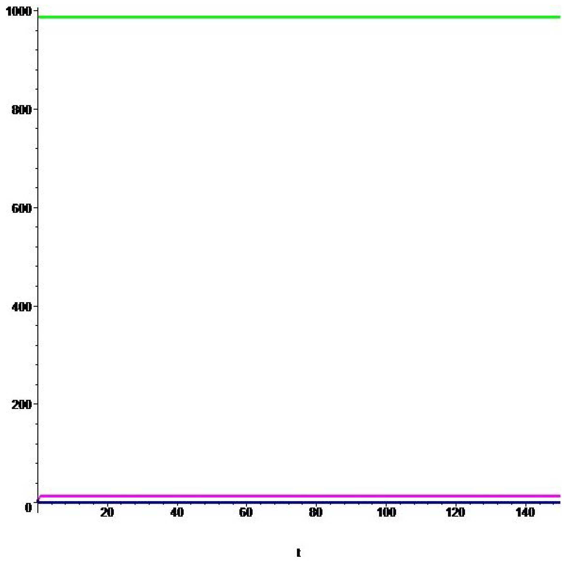
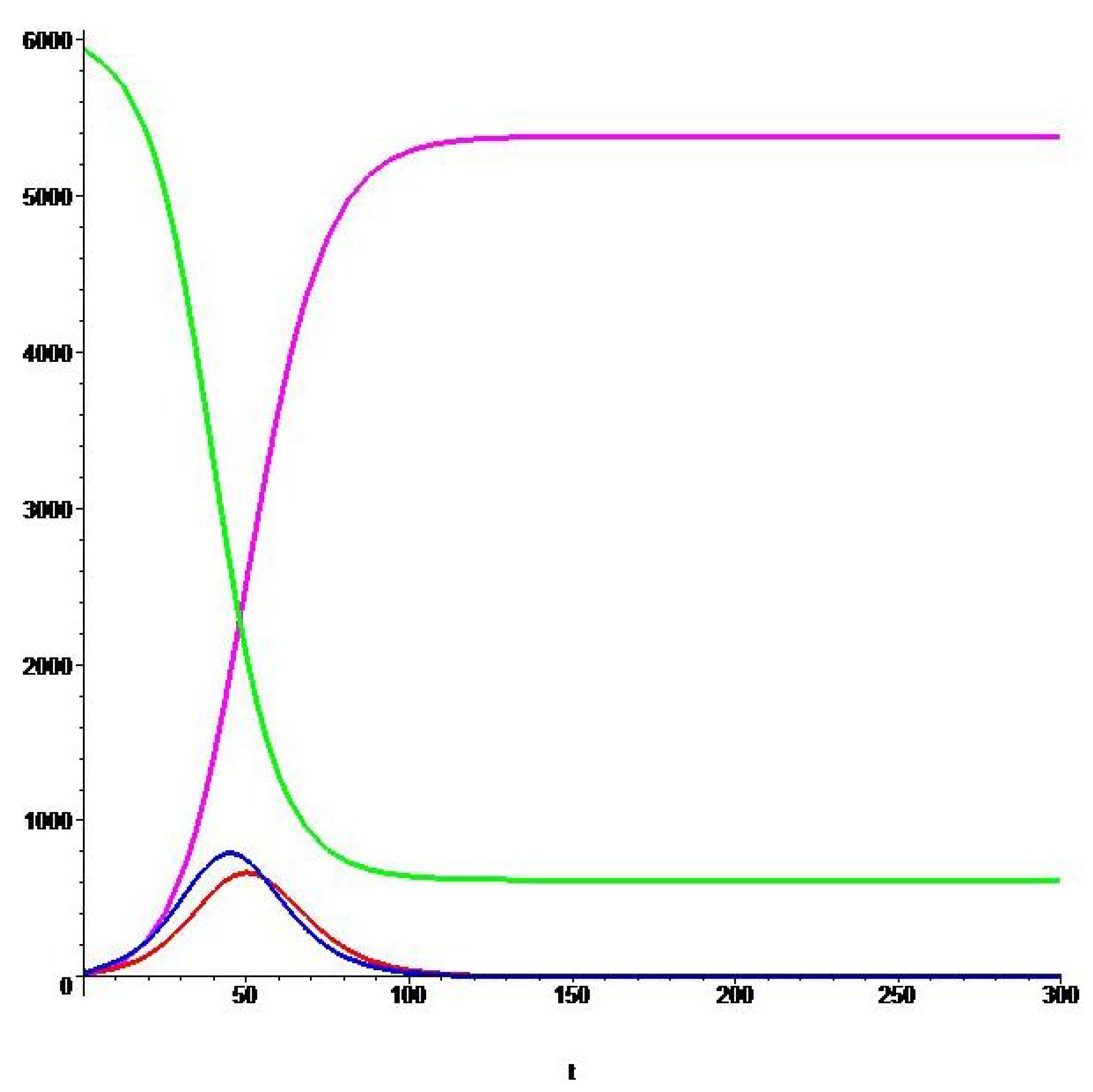
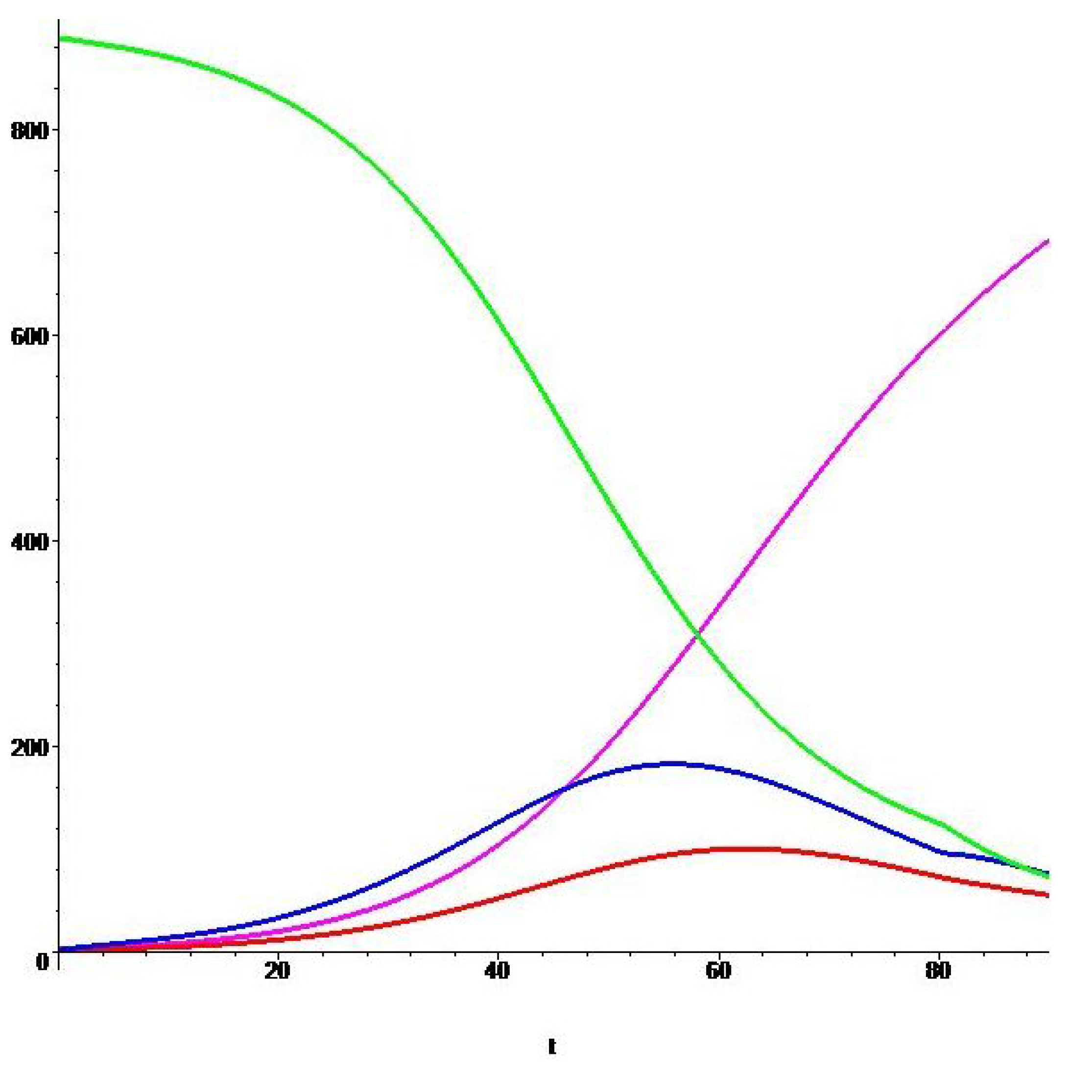
Figure 1, Figure 2 and Figure 3 show the graphs of the optimal solutions $S_{*}\left(t\right)$, $E_{*}\left(t\right)$, $I_{*}\left(t\right)$, $R_{*}\left(t\right)$ for Ebola epidemics in Zaire (1976), Uganda (2000), and Liberia (2014), respectively. The solution $S_{*}\left(t\right)$ is shown as a green curve, $E_{*}\left(t\right)$ as blue and $I_{*}\left(t\right)$ as a red curves, and, finally, the solution $R_{*}\left(t\right)$ is shown in magenta. 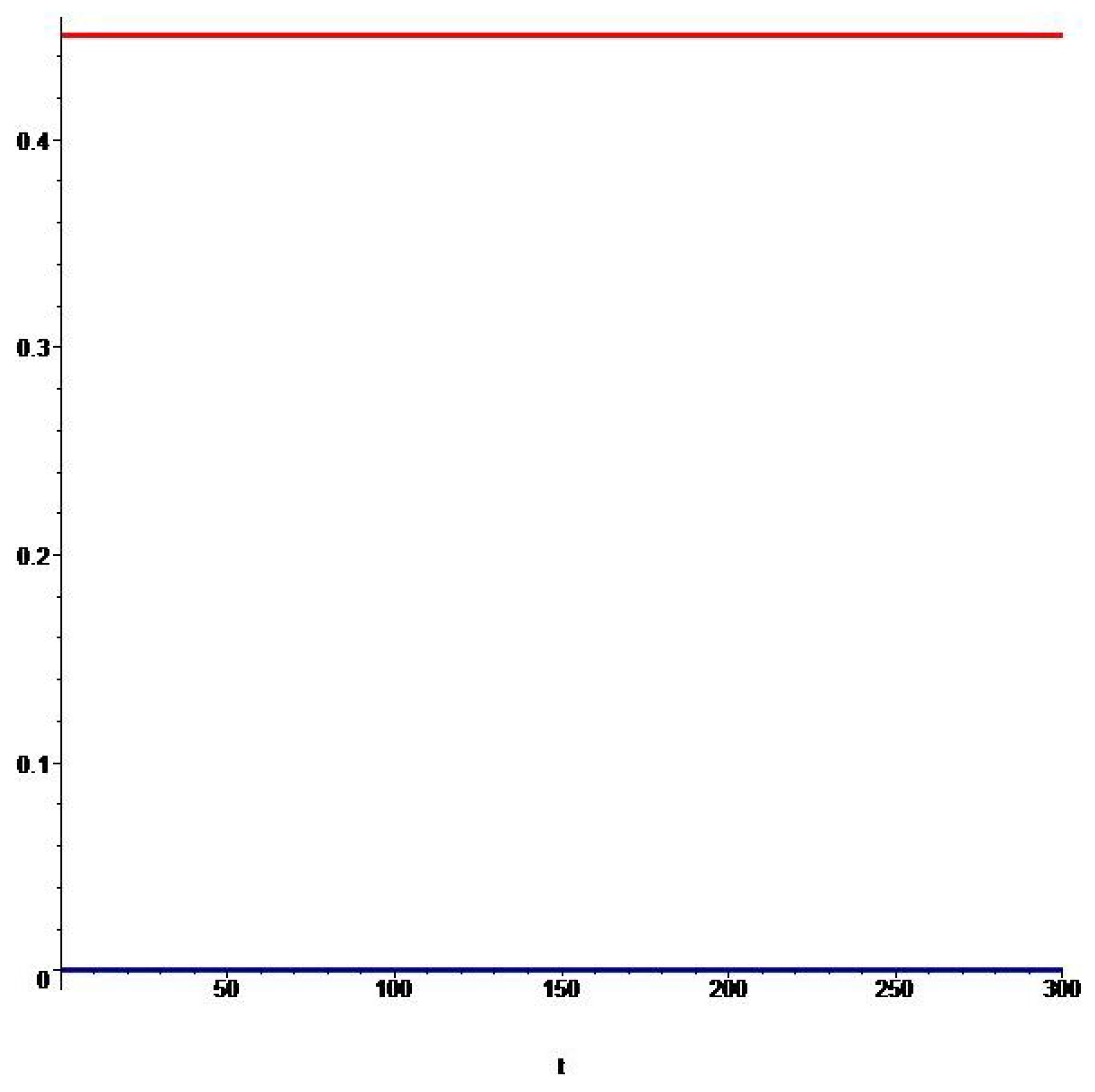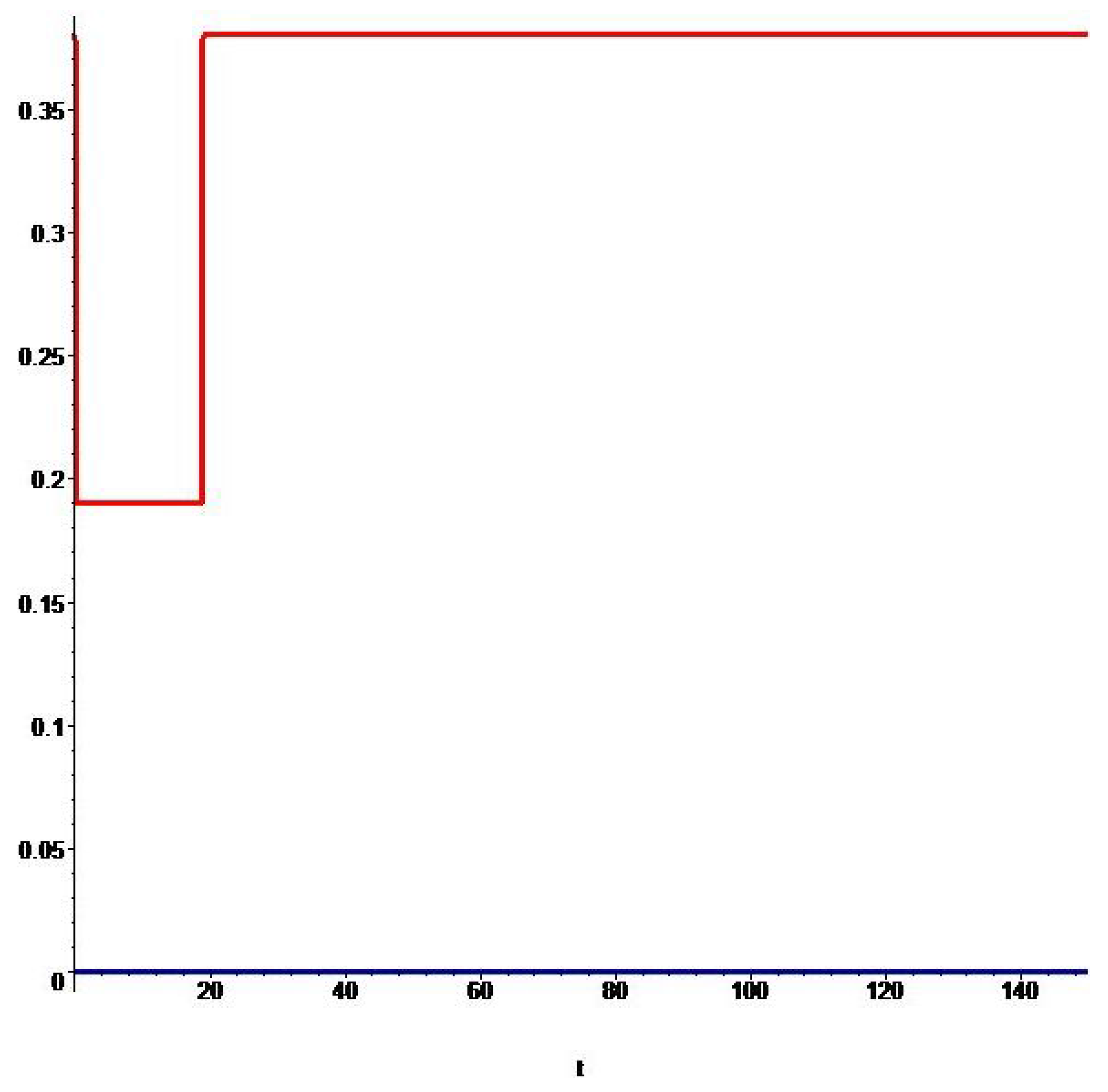Figure 4, Figure 5 and Figure 6 show the graphs of the corresponding optimal controls $u_{*}\left(t\right)$, $v_{*}\left(t\right)$. The control $u_{*}\left(t\right)$ is shown in red, and the control $v_{*}\left(t\right)$ is shown in blue. For these Ebola outbreaks, Table 2 shows the dependence of the values of the switchings ${\theta }_1^{*}$, ${\theta }_2^{*}$ of the controls $u_{*}\left(t\right)$, $v_{*}\left(t\right)$, and the optimal value of the functional ${\tilde{J}}_{*}=NJ(u_{*},v_{*})$ on the values of the weighting coefficients σ and ν.

Let us discuss the results presented by Table 2 and obtained for Zaire (1976). We can see that the type of the optimal controls $u_{*}\left(t\right)$, $v_{*}\left(t\right)$ for $0.01\le \sigma =\nu \le 0.1$ is very different from the type of these controls corresponding to $0.5\le \sigma =\nu \le 10$. In the first case, if $0.01\le \sigma =\nu \le 0.1$, the moments of switching ${\theta }_1^{*}$, ${\theta }_2^{*}$ of the controls $u_{*}\left(t\right)$, $v_{*}\left(t\right)$ are almost the same, which means that almost no intervention is needed in order to minimize the functional from (10), and all preventive control measures would take less than one day. In the second case, if $0.5\le \sigma =\nu \le 10$, the type of the optimal controls $u_{*}\left(t\right)$, $v_{*}\left(t\right)$ are qualitatively different, that is ${\theta }_1^{*}=0$, and the switching ${\theta }_2^{*}$ moves to the end of the interval $[0,T]$ as the values of the weighting coefficients σ, ν increase. In particular, if $\sigma =\nu =0.5$, active intervention control measures take place during the first 29–30 days, then they stop. If $\sigma =\nu =1$, then these measures continue at the maximum effort during the first 80–81 days. Finally, if $\sigma =\nu =10$, then intervention control measures continue at the maximum rate almost during the entire time interval (90 days). Note that similar behavior of the optimal controls $u_{*}\left(t\right)$, $v_{*}\left(t\right)$ can be observed for the Ebola outbreaks in Uganda (2000) and Liberia (2014). Such behavior of these controls is explained by the fact that the weighting coefficients σ and ν from formula (8) determine the relative importance of the functional $J_1(u,v)$ to $J_2(u,v)$. If the values of these weighting coefficients are small $(0.01\le \sigma =\nu \le 0.1)$, then the costs of intervention control constraints are relatively more important than the total fractions of exposed and infected individuals, and vice versa.

Figure 1. Graphs of the optimal solutions $S_{*}\left(t\right)$, $E_{*}\left(t\right)$, $I_{*}\left(t\right)$, $R_{*}\left(t\right)$ for the Ebola outbreak in Zaire (1976) for $\sigma =1$, $\nu =1$.

Figure 1. Graphs of the optimal solutions $S_{*}\left(t\right)$, $E_{*}\left(t\right)$, $I_{*}\left(t\right)$, $R_{*}\left(t\right)$ for the Ebola outbreak in Zaire (1976) for $\sigma =1$, $\nu =1$.

Figure 2. Graphs of the optimal solutions $S_{*}\left(t\right)$, $E_{*}\left(t\right)$, $I_{*}\left(t\right)$, $R_{*}\left(t\right)$ for the Ebola outbreak in Uganda (2000) for $\sigma =10$, $\nu =10$.

Figure 2. Graphs of the optimal solutions $S_{*}\left(t\right)$, $E_{*}\left(t\right)$, $I_{*}\left(t\right)$, $R_{*}\left(t\right)$ for the Ebola outbreak in Uganda (2000) for $\sigma =10$, $\nu =10$.

Figure 3. Graphs of the optimal solutions $S_{*}\left(t\right)$, $E_{*}\left(t\right)$, $I_{*}\left(t\right)$, $R_{*}\left(t\right)$ for the Ebola outbreak in Liberia (2014) for $\sigma =0.01$, $\nu =0.01$.

Figure 3. Graphs of the optimal solutions $S_{*}\left(t\right)$, $E_{*}\left(t\right)$, $I_{*}\left(t\right)$, $R_{*}\left(t\right)$ for the Ebola outbreak in Liberia (2014) for $\sigma =0.01$, $\nu =0.01$.

Figure 4. Graphs of the optimal controls $u_{*}\left(t\right)$, $v_{*}\left(t\right)$ for the Ebola outbreak in Zaire (1976) for $\sigma =1$, $\nu =1$.

Figure 4. Graphs of the optimal controls $u_{*}\left(t\right)$, $v_{*}\left(t\right)$ for the Ebola outbreak in Zaire (1976) for $\sigma =1$, $\nu =1$.

Figure 5. Graphs of the optimal controls $u_{*}\left(t\right)$, $v_{*}\left(t\right)$ for the Ebola outbreak in Uganda (2000) for $\sigma =10$, $\nu =10$.

Figure 5. Graphs of the optimal controls $u_{*}\left(t\right)$, $v_{*}\left(t\right)$ for the Ebola outbreak in Uganda (2000) for $\sigma =10$, $\nu =10$.

Figure 6. Graphs of the optimal controls $u_{*}\left(t\right)$, $v_{*}\left(t\right)$ for the Ebola outbreak in Liberia (2014) for $\sigma =0.01$, $\nu =0.01$.

Figure 6. Graphs of the optimal controls $u_{*}\left(t\right)$, $v_{*}\left(t\right)$ for the Ebola outbreak in Liberia (2014) for $\sigma =0.01$, $\nu =0.01$.

Table 2. Dependence of the optimal switchings ${\theta }_1^{*}$, ${\theta }_2^{*}$ and the optimal value ${\tilde{J}}_{*}$ from the parameters σ, ν.

	$\sigma =\nu$ $=0.01$	$\sigma =\nu$ $=0.05$	$\sigma =\nu$ $=0.1$	$\sigma =\nu$ $=0.5$	$\sigma =\nu$ $=1.0$	$\sigma =\nu$ $=10.0$
Zaire	${\theta }_1^{*}=41.10$	${\theta }_1^{*}=72.00$	${\theta }_1^{*}=70.20$	${\theta }_1^{*}=0.000$	${\theta }_1^{*}=0.000$	${\theta }_1^{*}=0.000$
(1976)	${\theta }_2^{*}=41.40$	${\theta }_2^{*}=72.30$	${\theta }_2^{*}=70.50$	${\theta }_2^{*}=29.40$	${\theta }_2^{*}=80.40$	${\theta }_2^{*}=89.10$
	${\tilde{J}}_{*}=168.1$	${\tilde{J}}_{*}=840.3$	${\tilde{J}}_{*}=1680.5$	${\tilde{J}}_{*}=8345.2$	${\tilde{J}}_{*}=15,515.2$	${\tilde{J}}_{*}=138,231.4$
Uganda	${\theta }_1^{*}=14.10$	${\theta }_1^{*}=31.20$	${\theta }_1^{*}=23.40$	${\theta }_1^{*}=9.000$	${\theta }_1^{*}=35.10$	${\theta }_1^{*}=0.000$
(2000)	${\theta }_2^{*}=16.20$	${\theta }_2^{*}=39.60$	${\theta }_2^{*}=29.40$	${\theta }_2^{*}=9.900$	${\theta }_2^{*}=149.70$	${\theta }_2^{*}=18.90$
	${\tilde{J}}_{*}=0.0314$	${\tilde{J}}_{*}=0.1571$	${\tilde{J}}_{*}=0.3142$	${\tilde{J}}_{*}=1.5711$	${\tilde{J}}_{*}=3.1421$	${\tilde{J}}_{*}=30.126$
Liberia	${\theta }_1^{*}=58.80$	${\theta }_1^{*}=59.10$	${\theta }_1^{*}=0.000$	${\theta }_1^{*}=0.000$	${\theta }_1^{*}=0.000$	${\theta }_1^{*}=0.000$
(2014)	${\theta }_2^{*}=59.10$	${\theta }_2^{*}=59.40$	${\theta }_2^{*}=286.2$	${\theta }_2^{*}=296.7$	${\theta }_2^{*}=298.2$	${\theta }_2^{*}=299.7$
	${\tilde{J}}_{*}=637.9$	${\tilde{J}}_{*}=3189.7$	${\tilde{J}}_{*}=5858.7$	${\tilde{J}}_{*}=17,219.2$	${\tilde{J}}_{*}=31,413.1$	${\tilde{J}}_{*}=286,889.3$

Table 2. Dependence of the optimal switchings ${\theta }_1^{*}$, ${\theta }_2^{*}$ and the optimal value ${\tilde{J}}_{*}$ from the parameters σ, ν.

	$\sigma =\nu$ $=0.01$	$\sigma =\nu$ $=0.05$	$\sigma =\nu$ $=0.1$	$\sigma =\nu$ $=0.5$	$\sigma =\nu$ $=1.0$	$\sigma =\nu$ $=10.0$
Zaire	${\theta }_1^{*}=41.10$	${\theta }_1^{*}=72.00$	${\theta }_1^{*}=70.20$	${\theta }_1^{*}=0.000$	${\theta }_1^{*}=0.000$	${\theta }_1^{*}=0.000$
(1976)	${\theta }_2^{*}=41.40$	${\theta }_2^{*}=72.30$	${\theta }_2^{*}=70.50$	${\theta }_2^{*}=29.40$	${\theta }_2^{*}=80.40$	${\theta }_2^{*}=89.10$
	${\tilde{J}}_{*}=168.1$	${\tilde{J}}_{*}=840.3$	${\tilde{J}}_{*}=1680.5$	${\tilde{J}}_{*}=8345.2$	${\tilde{J}}_{*}=15,515.2$	${\tilde{J}}_{*}=138,231.4$
Uganda	${\theta }_1^{*}=14.10$	${\theta }_1^{*}=31.20$	${\theta }_1^{*}=23.40$	${\theta }_1^{*}=9.000$	${\theta }_1^{*}=35.10$	${\theta }_1^{*}=0.000$
(2000)	${\theta }_2^{*}=16.20$	${\theta }_2^{*}=39.60$	${\theta }_2^{*}=29.40$	${\theta }_2^{*}=9.900$	${\theta }_2^{*}=149.70$	${\theta }_2^{*}=18.90$
	${\tilde{J}}_{*}=0.0314$	${\tilde{J}}_{*}=0.1571$	${\tilde{J}}_{*}=0.3142$	${\tilde{J}}_{*}=1.5711$	${\tilde{J}}_{*}=3.1421$	${\tilde{J}}_{*}=30.126$
Liberia	${\theta }_1^{*}=58.80$	${\theta }_1^{*}=59.10$	${\theta }_1^{*}=0.000$	${\theta }_1^{*}=0.000$	${\theta }_1^{*}=0.000$	${\theta }_1^{*}=0.000$
(2014)	${\theta }_2^{*}=59.10$	${\theta }_2^{*}=59.40$	${\theta }_2^{*}=286.2$	${\theta }_2^{*}=296.7$	${\theta }_2^{*}=298.2$	${\theta }_2^{*}=299.7$
	${\tilde{J}}_{*}=637.9$	${\tilde{J}}_{*}=3189.7$	${\tilde{J}}_{*}=5858.7$	${\tilde{J}}_{*}=17,219.2$	${\tilde{J}}_{*}=31,413.1$	${\tilde{J}}_{*}=286,889.3$

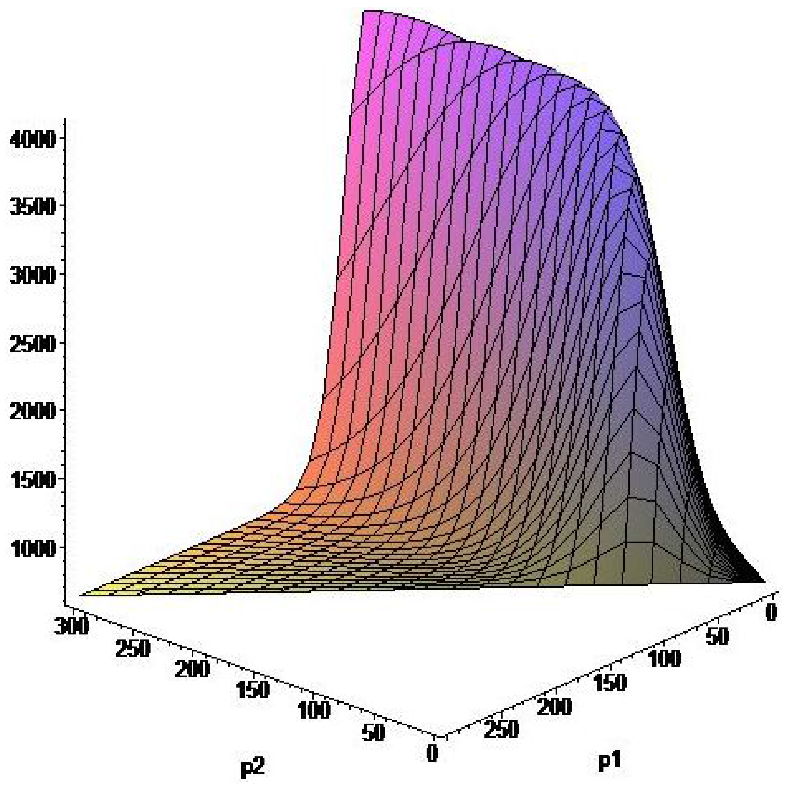
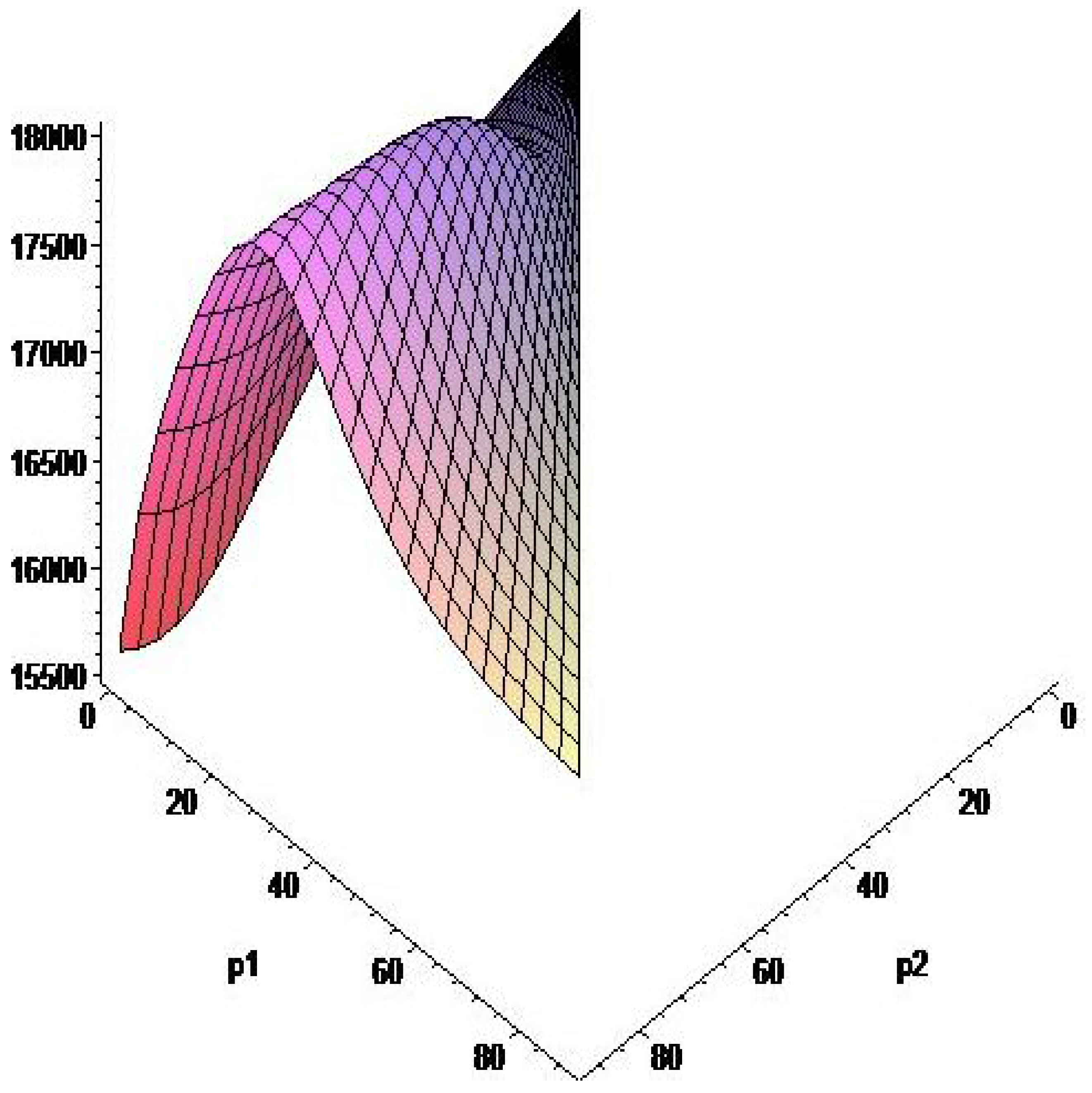
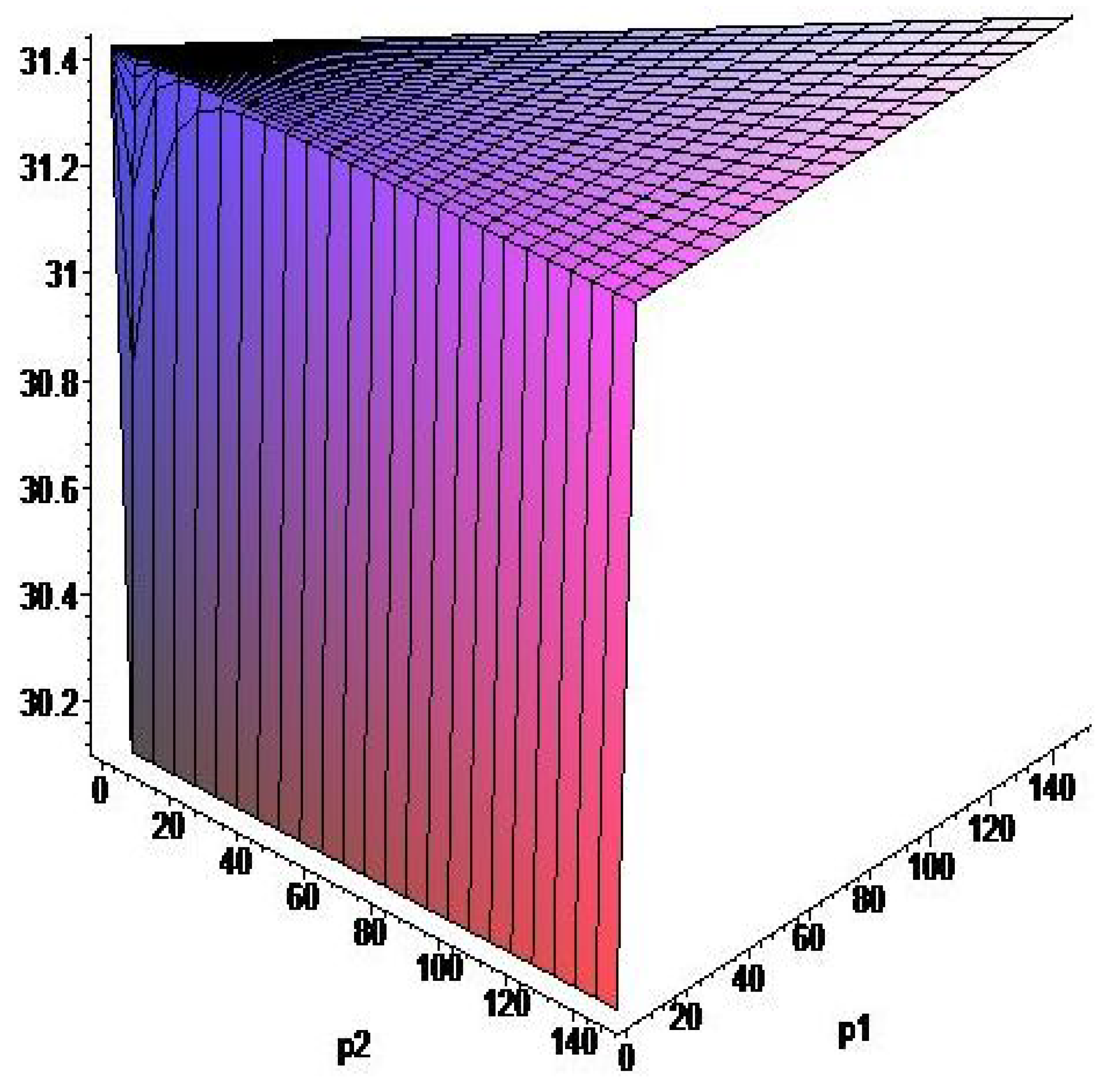
Finally, Figure 7, Figure 8 and Figure 9 represent the surfaces describing the dependence of values of the function $\tilde{J}\left(\theta \right)=NJ(u_{\theta },v_{\theta })$ on the moments of switching $\theta ={({\theta }_1,{\theta }_2)}^{\top }\in \Omega$. One of the points of such surfaces correspond to the optimal values ${\tilde{J}}_{*}$. Analyzing these surfaces it is easy to see that the function $\tilde{J}\left(\theta \right)$ has not only the global minimum, the search of which is the subject of our investigation, but also local minima. This once again demonstrates that the Pontryagin maximum principle is only a necessary optimality condition.

Figure 7. Surface $\tilde{J}\left(\theta \right)$ for the Ebola outbreak in Zaire (1976) for $\sigma =1$, $\nu =1$.

Figure 7. Surface $\tilde{J}\left(\theta \right)$ for the Ebola outbreak in Zaire (1976) for $\sigma =1$, $\nu =1$.

Figure 8. Surface $\tilde{J}\left(\theta \right)$ for the Ebola outbreak in Uganda (2000) for $\sigma =10$, $\nu =10$.

Figure 8. Surface $\tilde{J}\left(\theta \right)$ for the Ebola outbreak in Uganda (2000) for $\sigma =10$, $\nu =10$.

Figure 9. Surface $\tilde{J}\left(\theta \right)$ for the Ebola outbreak in Liberia (2014) for $\sigma =0.01$, $\nu =0.01$.

Figure 9. Surface $\tilde{J}\left(\theta \right)$ for the Ebola outbreak in Liberia (2014) for $\sigma =0.01$, $\nu =0.01$.

8. Conclusions

In this paper, a problem of minimizing the weighted sum of total fractions of infected and exposed individuals and total costs of intervention control constraints over a given time interval for the SEIR control model describing the spread of an Ebola epidemic in a population of a constant size was considered. Analysis of the optimal solutions of this problem was made using the Pontryagin maximum principle. The established properties of the switching function allowed the reduction of the original optimal control problem to the solution of the problem of a constrained minimization of the function of two variables. Results of the numerical calculations and their analysis are presented.