1. Introduction
In the last two decades, synchronization and anti-synchronization (AS) of chaotic systems have attracted considerable attention due to the potential applications in different scientific areas, such as secure communications [
1], image encryption [
2], laser technology [
3], physical systems [
4], and artificial neural networks [
5]. As a result, a wide range of synchronization and AS control techniques and methods have been proposed. These include sliding mode control [
6], active control [
7], non-linear control [
8], periodically intermittent control [
9], adaptive control [
10], H-∞ synchronization [
11], projective synchronization [
12], and generalized synchronization [
13],
etc. Anti-synchronization (AS) is a special form of generalized synchronization. AS is a mechanism in which the state vectors of the two synchronized chaotic systems have the same amplitude but opposite signs. That is, the sum of two signals converges to zero when the AS phenomenon appears. AS has successful applications in different scientific disciplines [
14,
15]. It has been experimentally, as well as numerically confirmed, that the two coupled chaotic systems can achieve AS [
16,
17]. The AS phenomenon in non-equilibrium systems suggests that it can be used as a technique for particle separation in a mixture of interacting particles [
17]. A current study of using AS control of lasers, one can generate not only drop-outs in intensity but also short high-intensity pulses, and this results in pulses of particular shapes [
18].
In recent years, anti-synchronization of chaotic systems with different dimensions has been reported in the literature [
19,
20,
21]. Two types of AS have been discussed, namely reduced order AS [
20] and increased order AS [
21]. Mossa and Noorani [
20] presented the idea of reduced order AS of chaotic systems with uncertain parameters. Using the adaptive control strategy based on the Lyapunov stability theory [
22], the same authors [
21] studied the increased order AS of uncertain hyperchaotic Lu and chaotic Lu systems.
However, the finding of these results [
20,
21] are limited to the asymptotic stability of the resulting AS behavior. This means that the corresponding state trajectories of the two coupled chaotic systems are anti-synchronized in an infinite settling time. In addition, the proposed reduced (increased) order AS of chaotic systems has been achieved without considering the effect of both model uncertainties and external disturbances. These results [
20,
21] would have been more interesting if it had included the finite-time AS behavior rather than merely asymptotic stability under the effect of both model uncertainties and external disturbances.
In real applications, it has been reported [
22] that the finite-time AS stability is important to chaotic systems as the systems are required for AS quickly as possible. In case of chaotic systems with different dimensions, both systems have different topological properties and the traces changes in their respective trajectories with time are different. These properties of chaotic systems with different dimensions increase security in the communication channel and, therefore, require an effective approach to anti-synchronize chaotic systems with different dimensions in a finite-time.
Motivated by the aforesaid discussion, the purpose of this article is to make an innovative contribution in this direction. In this article, the authors study finite-time reduced (increased)-order AS behavior between two chaotic systems under the effect of both unknown model uncertainties and external disturbances. Using the master-slave system AS scheme, a generalized feedback control scheme will be proposed that would guarantee finite-time reduced (increased) order AS globally. Two illustrative examples are given to verify the robustness and performance of the proposed finite-time AS approach: finite-time reduced order AS between the hyperchaotic Li [
23] and the chaotic Lu [
24] systems and finite-time increased order AS between the chaotic Lu and the hyperchaotic Li systems. To the best of the authors’ knowledge, no attempt has been made for the robust finite-time AS scheme for chaotic systems with different dimensions and this has remained an open problem.
The remainder of the paper is organized as follows:
Section 2 presents a brief descriptions of the hyperchaotic Li and the chaotic Lu systems. In
Section 3, the problem of finite-time reduced-order AS between the hyperchaotic Li and the chaotic Lu systems is solved. Accordingly,
Section 4 is devoted to solve the finite-time increased-order AS problem between the chaotic Lu and the hyperchaotic Li systems. The paper concludes in
Section 5.
3. Finite-Time Reduced Order Anti-Synchronization Scheme
3.1. Some Basic Preliminaries and Lemmas
Lemma 1 [
25]. For any
and
, the following inequality holds true:
Proof of Lemma 1. Consider the following inequality:
Which holds true for
being the arithmetic and geometric means respectively. Now substituting
to the above inequality Equation (3) that yields the following form:
Lemma 2. If
, then, the following inequality holds true:
Proof of Lemma 2. Let us assumed the following function defined as:
then,
Since , it follows that .
If
then, substituting
in Equation (6) that yields:
Lemma 3 [
26]. Assume that there exists a continuous positive definite function
such that
is radially unbounded and satisfies the following differential inequality:
where
and
are two constant numbers. Then, for any
satisfies the following inequality:
and
Then, the origin is globally stable in the finite-time
. The settling time
is given as follows:
3.2. Problem Statement
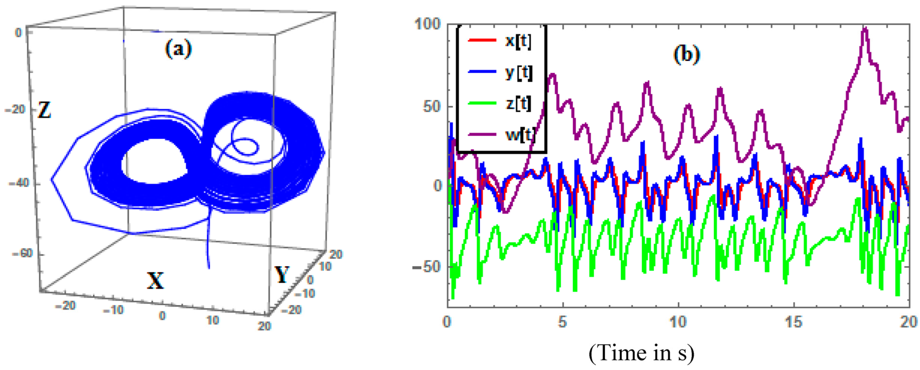
To achieve finite-time reduced-order AS between the hyperchaotic Li and chaotic Lu systems, it is assumed that the projection part of the hyperchaotic Li system is considered as the master system and is described as follows:
where
are the state variables,
are the corresponding control parameters of the master system Equation (10), respectively.
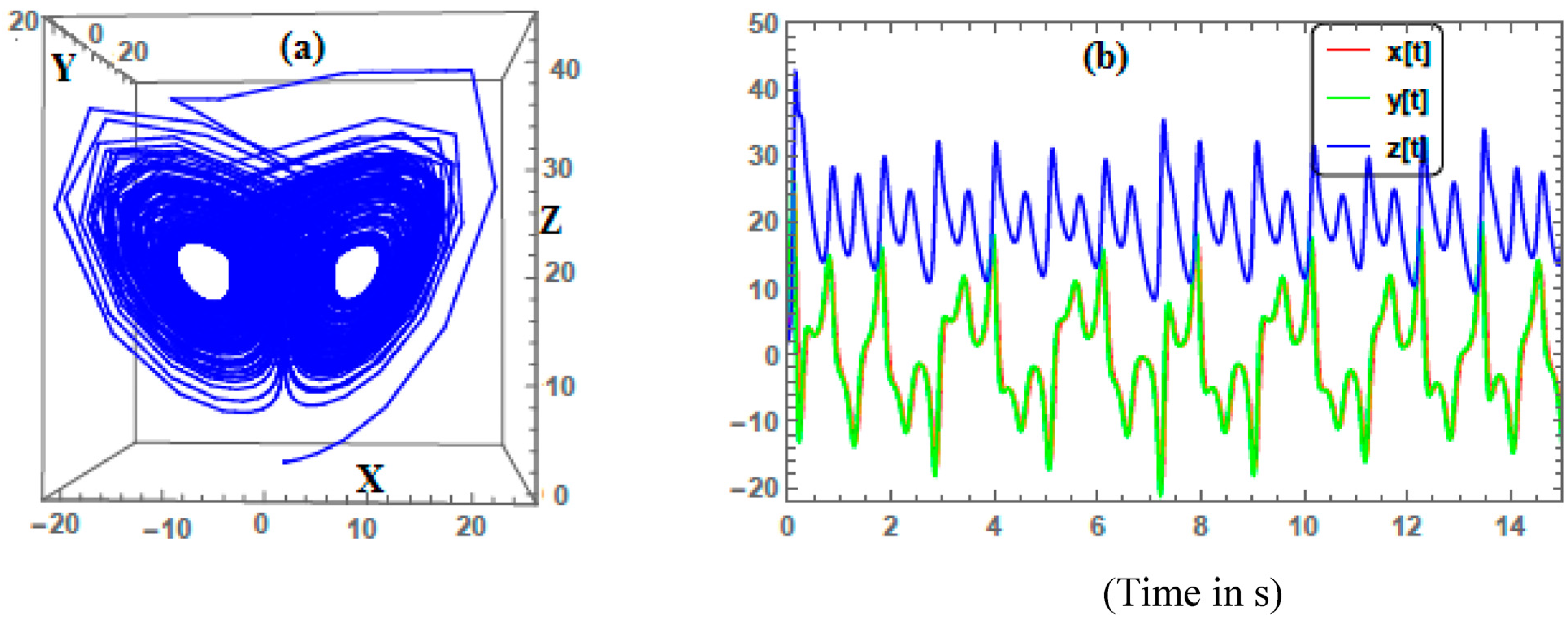
are the unknown model uncertainties and external disturbances present in the master system. Likewise, the Lu chaotic system is considered as the slave system and is described as follows:
where
are the state variables,
are the corresponding control parameters of the slave system respectively.
are the unknown model uncertainties and external disturbances present in the slave system, and
is the control input that is yet to be deigned.
Let
be the AS error vector. Then, the time varying AS error system of the master (10) and slave (11) systems is described as below:
Under these circumstances, it is desired to design a feedback controller that synthesis a smooth control input . This control inputs accomplishes the reduced order AS within finite-time .
The reduced order AS objectives are summarized as follows:
Objective 1. The reduced order AS scheme accomplishes if:
Objective 2. The reduced order AS error dynamical system (12) are globally stable in the finite-time given by Equation (16).
Assumption 1. Since chaotic trajectories are always bounded, there exist a positive constant
such that [
25]:
Assumption 2. It is assumed that the unknown model uncertainties and external disturbances are Norm-bounded [
27]. That is:
Accordingly, it is concluded that:
where
are unknown positive constants.
3.3. Controller Design
Theorem 1. For the arbitrary initial conditions,
; of the master and slave systems respectively, the error system Equation (12) will converge to zero globally under the control law given by:
in the finite-time
determined by the following:
Then, objectives one and two are accomplished.
Proof of Theorem 1. Construct a Lyapunov function candidate as follows:
where
is a positive definite function. Now calculate the time derivatives of
along the trajectories of the error system Equation (12) that yields:
Now introducing the control inputs,
Equation (15) to the right hand side of Equation (18) yields:
Using Lemma 1, Equation (19) yields:
where
are two positive constants. Let us choose
as follows:
Using Equation (21), then, Equation (20) becomes as follows:
Using Lemma 2 to the above Equation (22), we obtain the following inequality:
Thus, according to Lemma 3, the AS error system Equation (12) will converge to zero in the finite-time . Accordingly, the slave chaotic Lu system will synchronize globally with the projection part of the hyperchaotic Li system in the finite-time .
3.4. Simulation and Results
In this sub-section of the article, numerical simulation results using Mathematica 10
v (Nizwa, Oman) are provided to verify the robustness and effectiveness of the proposed finite-time reduced order AS approach. Parameters of the hyperchaotic Li Equation (1) and the chaotic Lu Equation (2) systems which are set as:
, respectively. The initial states of the master and slave systems being taken as:
and
respectively. According to the Theorem 1, the linear controller gains
are chosen as
and the constant number
being taken as
. In numerical simulation, the following unknown model uncertainties and external disturbances are applied to the master Equation (10) and slave Equation (11) systems respectively:
As a result, one can obtain . The corresponding numerical results are as follows.
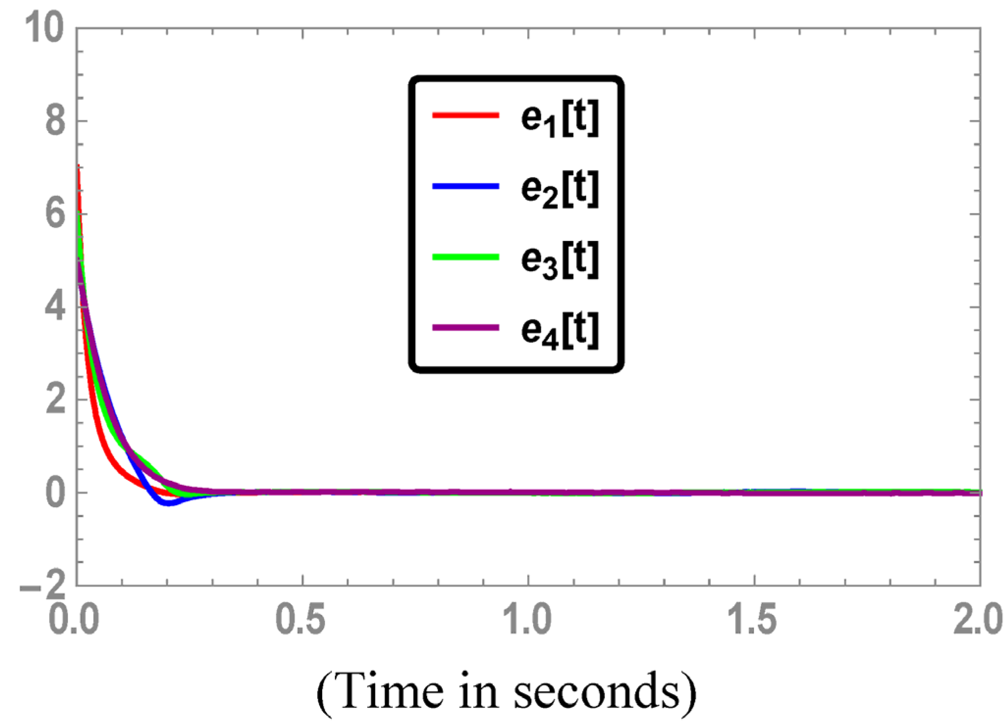
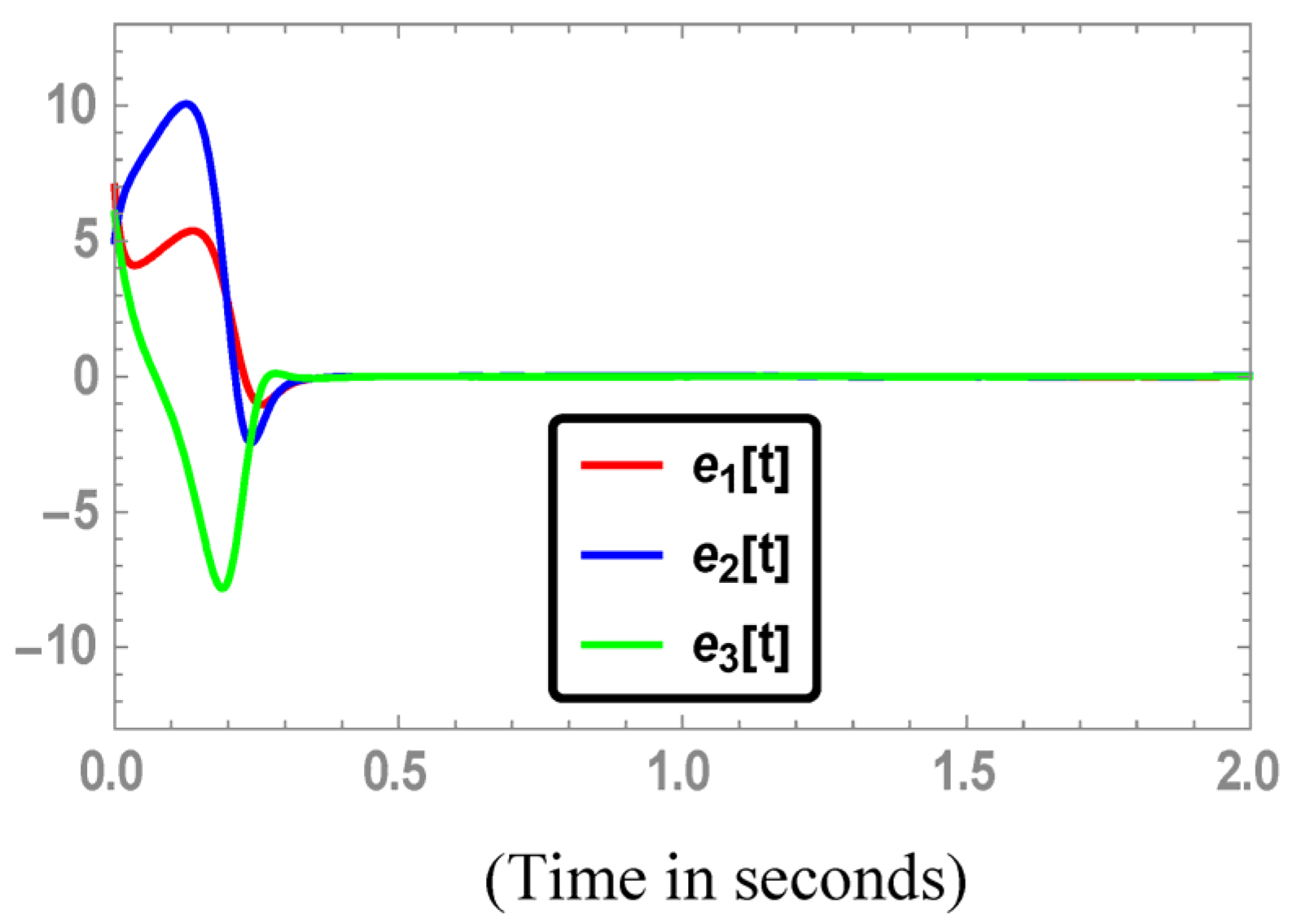
Figure 3, depicts the time series of the convergence of the reduce order AS error signals to the zero state. As expected, one can observe that the AS error signals converged to the zero state quickly, which demonstrates the robustness and performance of the control action Equation (15) for the finite-time reduced-order AS scheme.
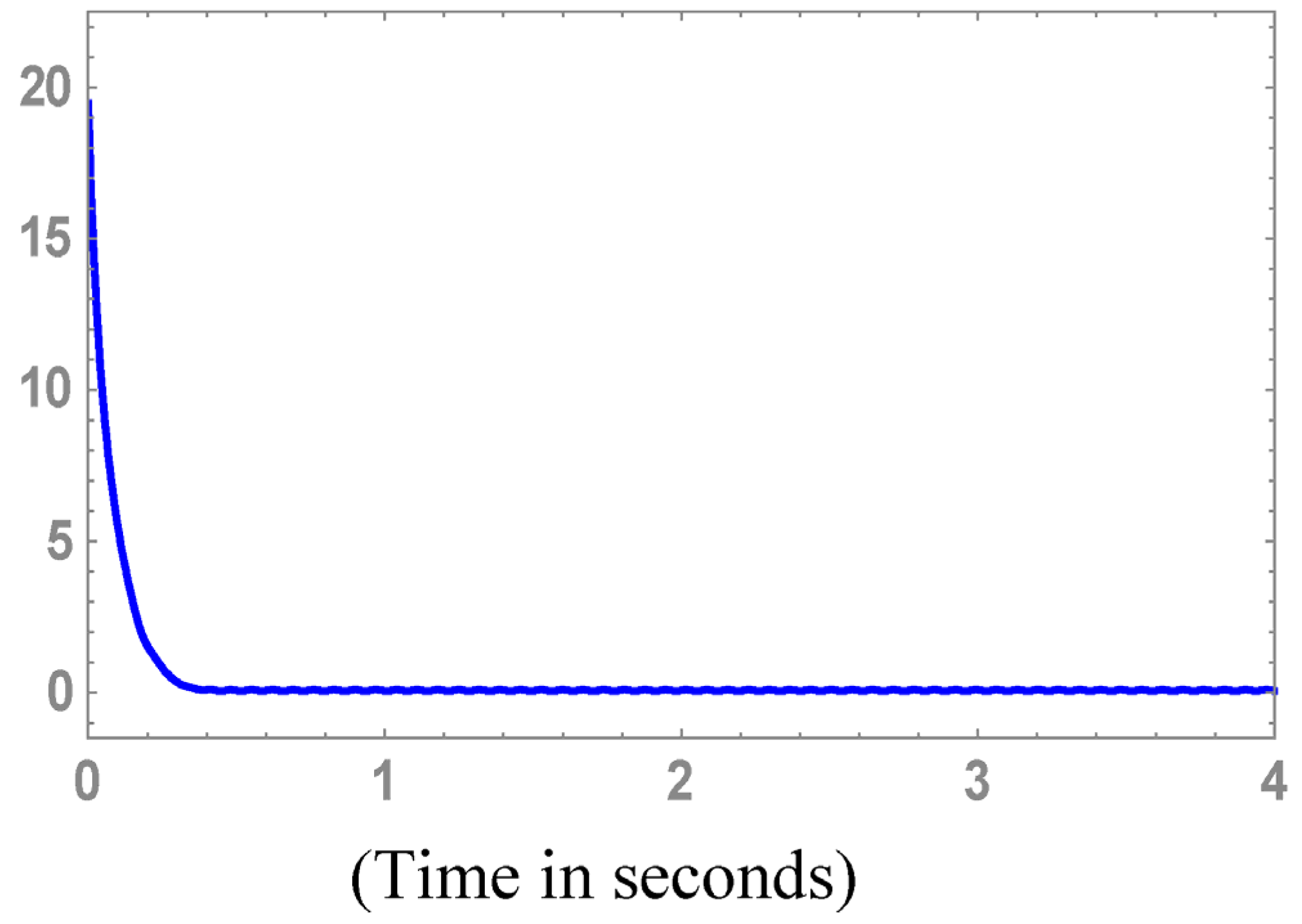
Figure 4, illustrates the time series of the finite-time
Equation (16). From the main Theorem 1, it can be checked that slave system Equation (11) is anti-synchronized with the projection part of the master system Equation (10) in the finite-time, when the control inputs are activated at
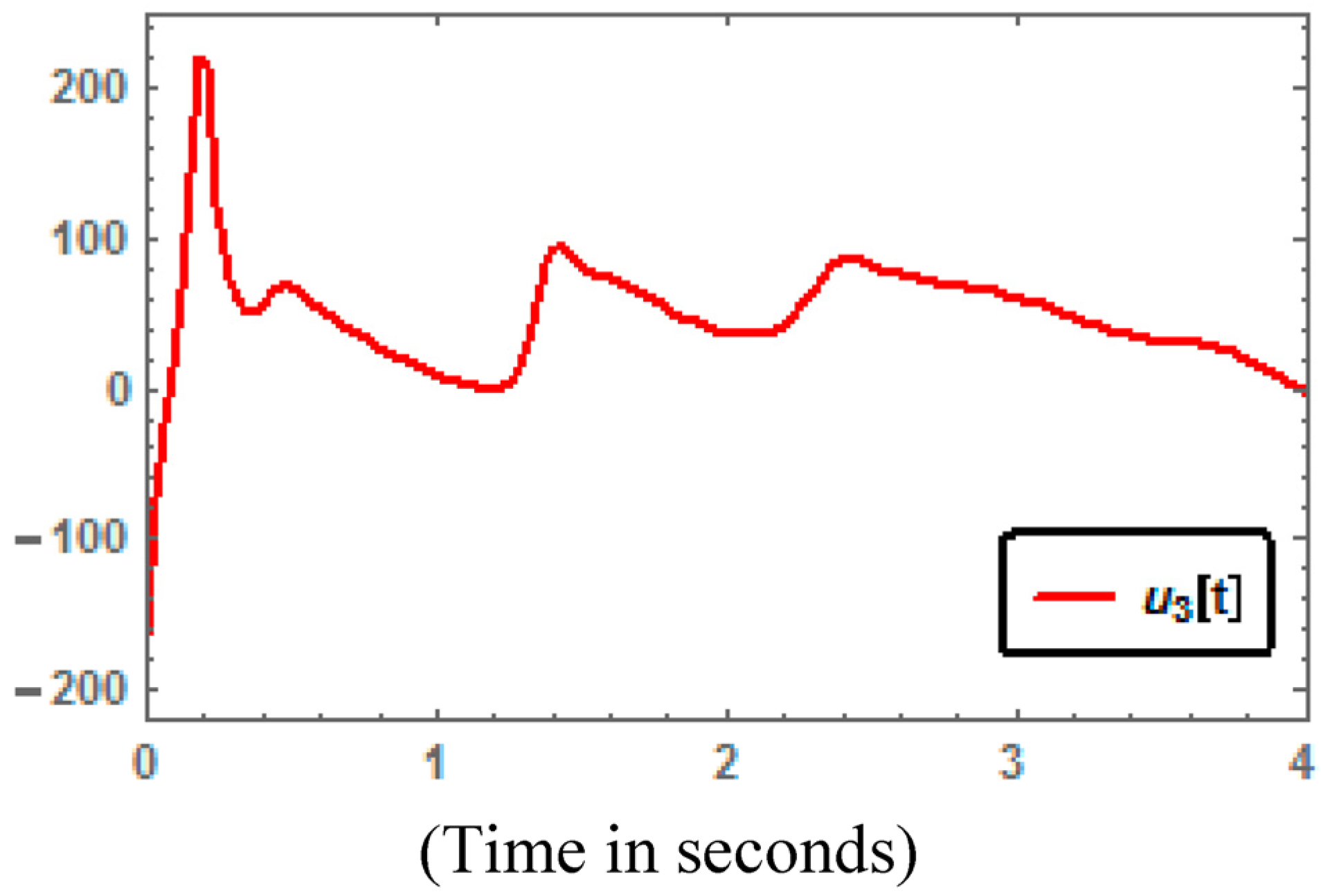
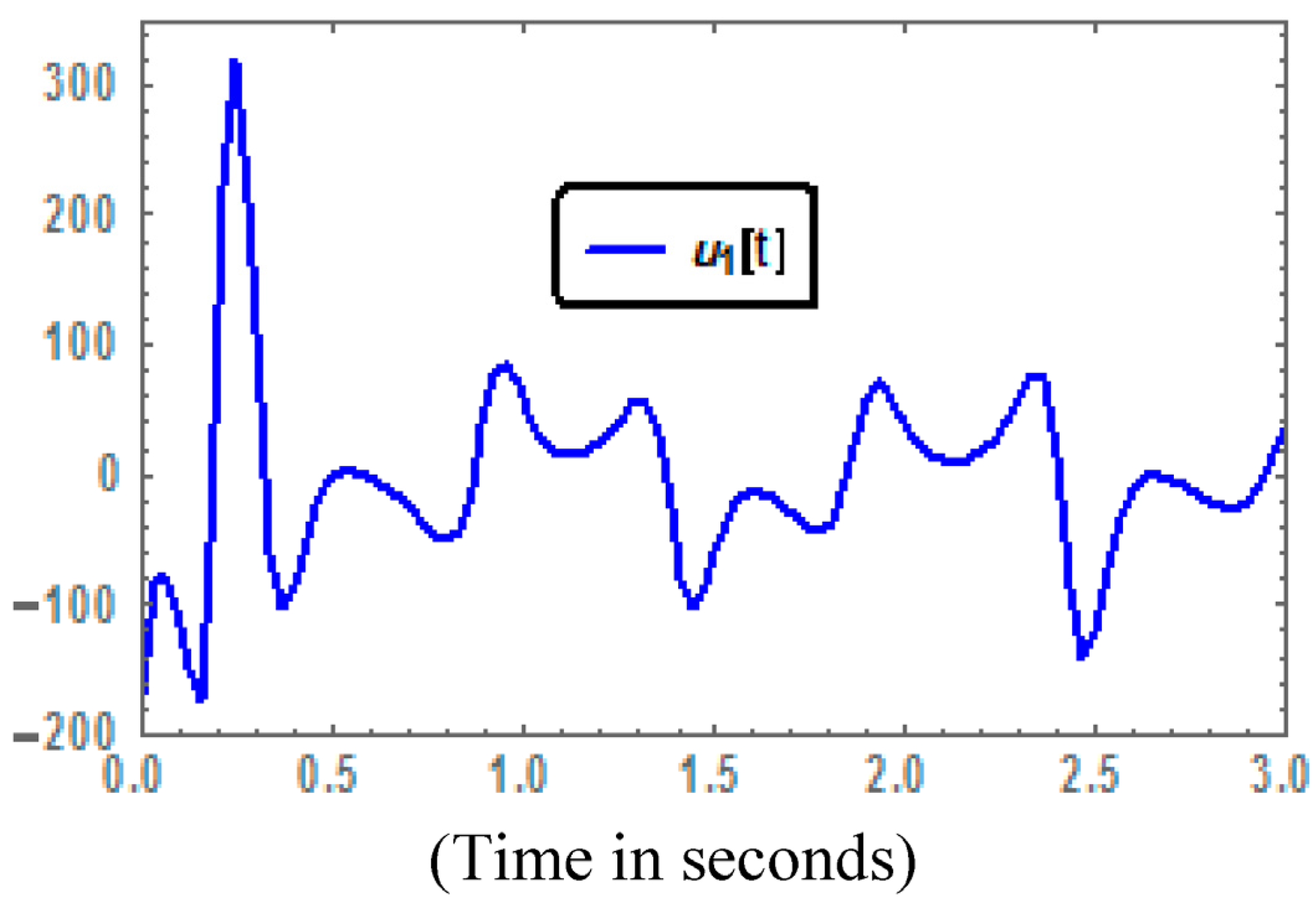
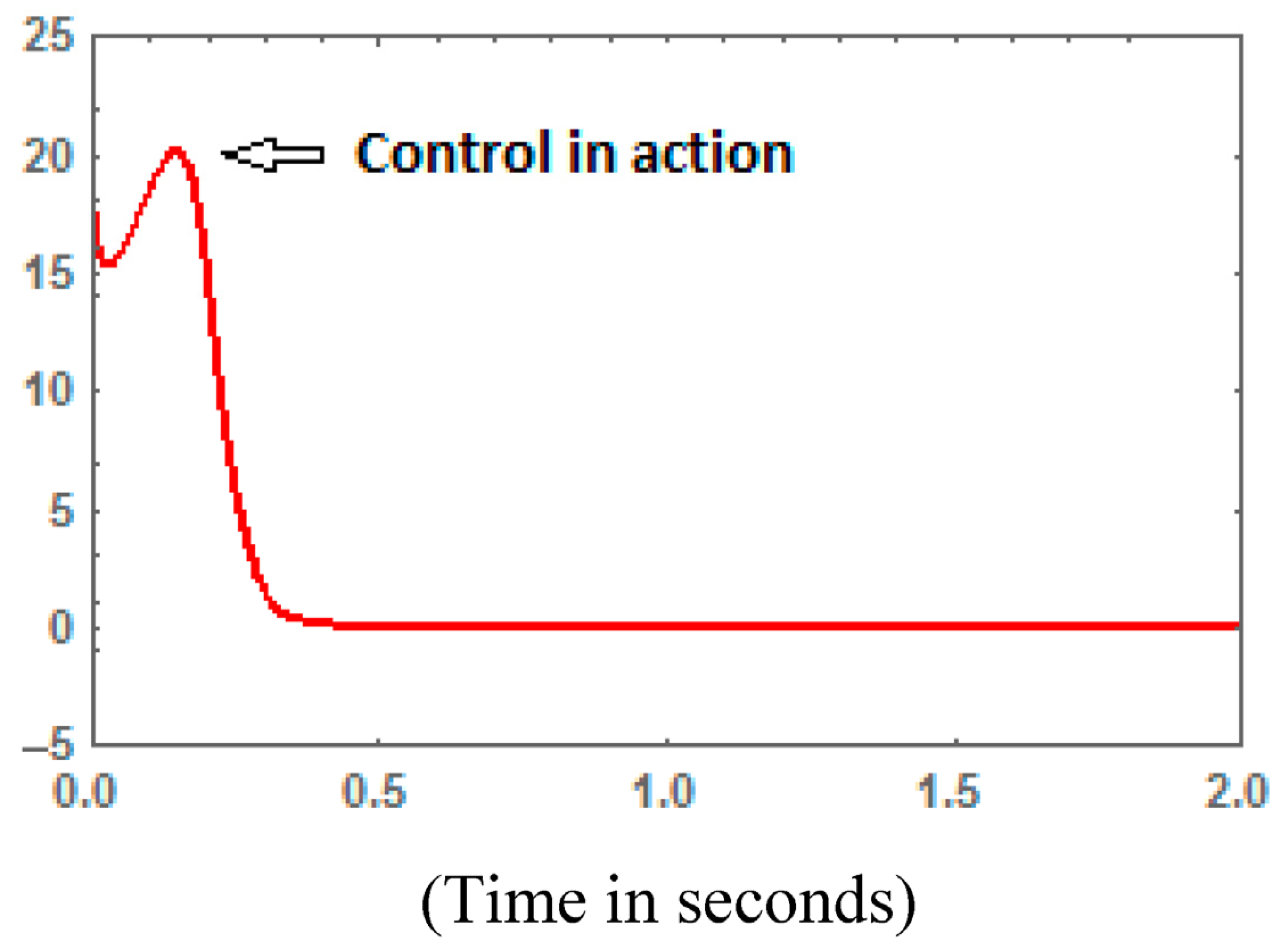
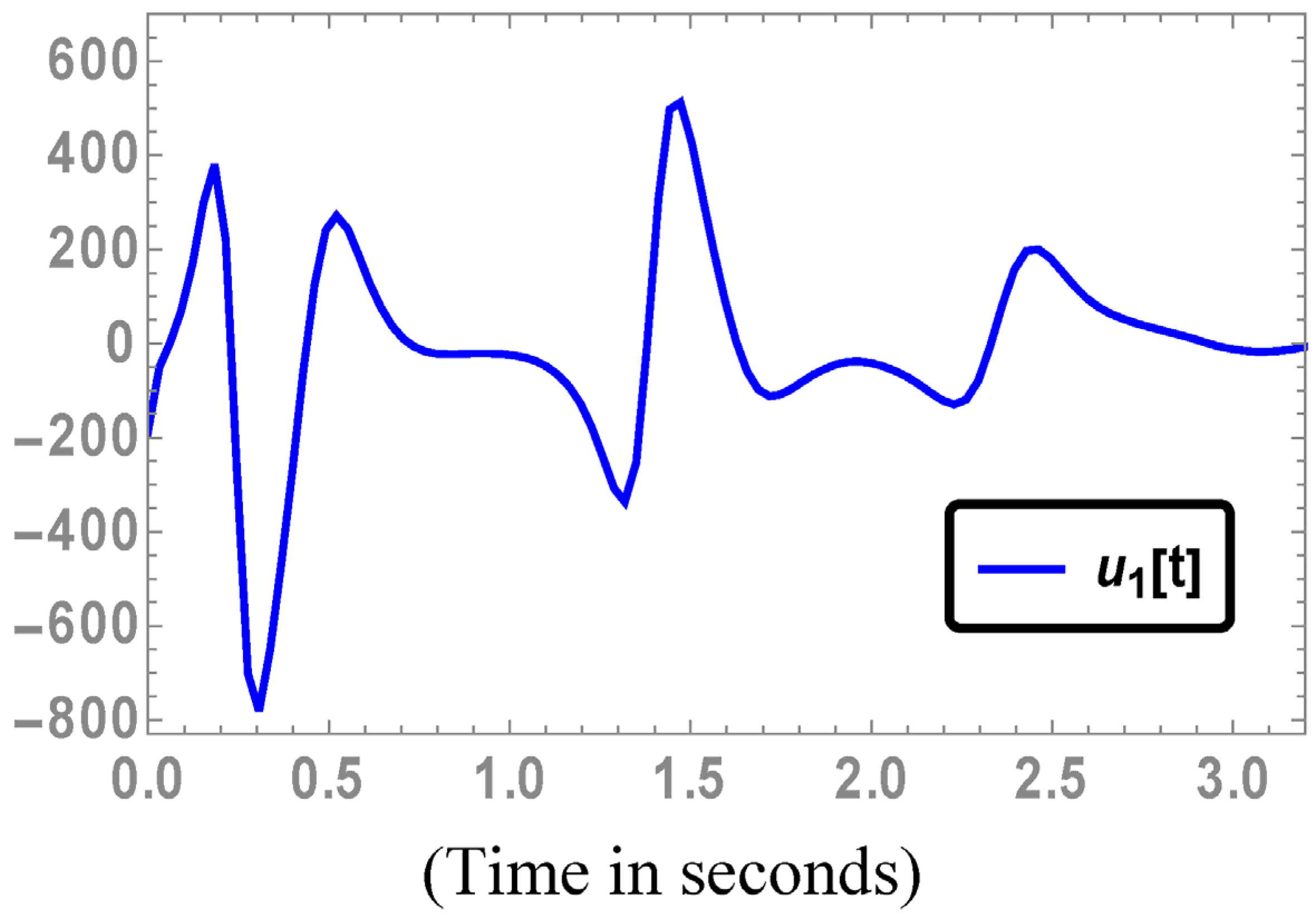
. Time series of the control inputs are depicted in
Figure 5,
Figure 6 and
Figure 7.
Figure 3.
Times series of the AS error signals.
Figure 3.
Times series of the AS error signals.
Figure 4.
Time series of the estimated finite-time .
Figure 4.
Time series of the estimated finite-time .
Figure 5.
Times series of the control input .
Figure 5.
Times series of the control input .
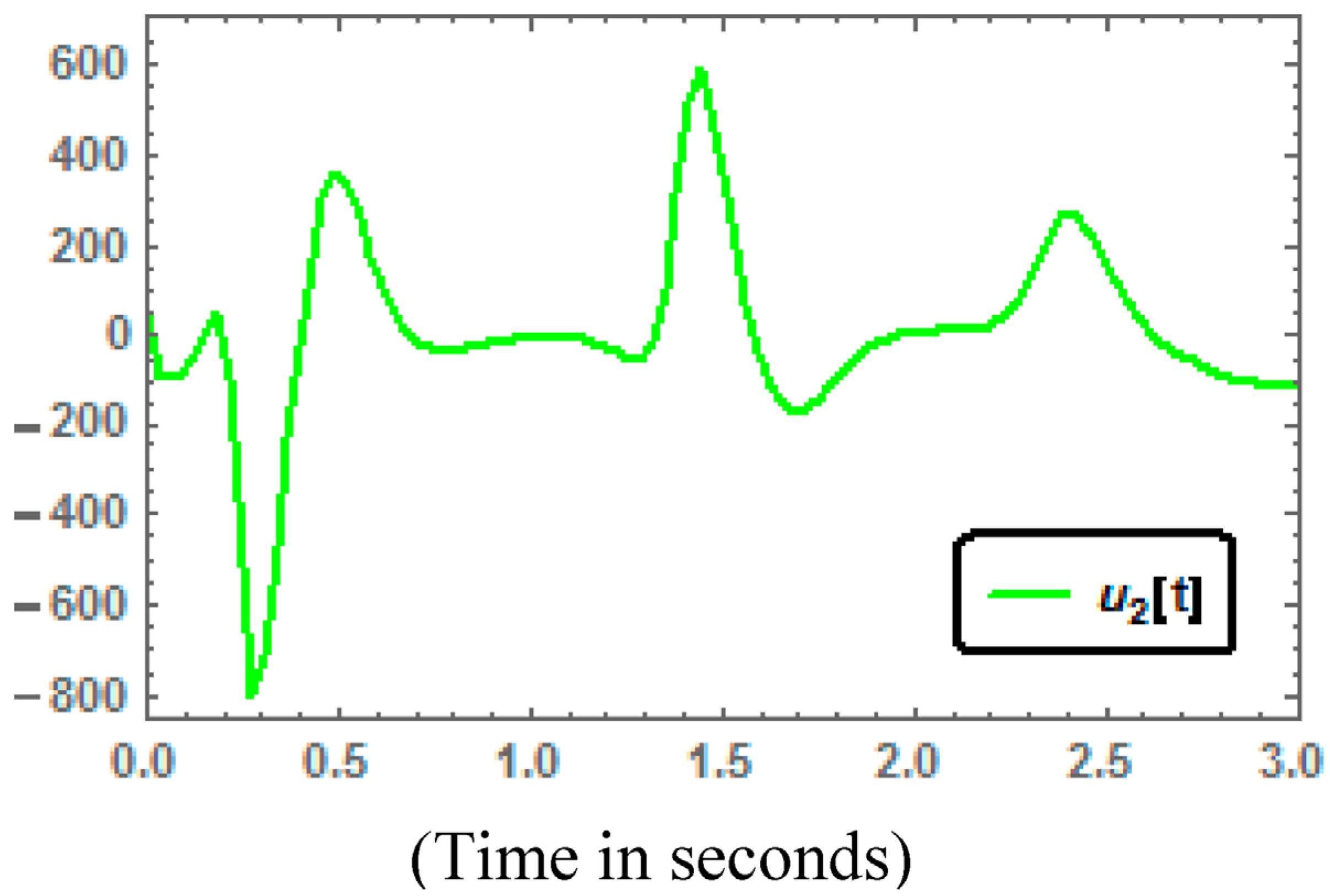
Figure 6.
Time series of the control input .
Figure 6.
Time series of the control input .
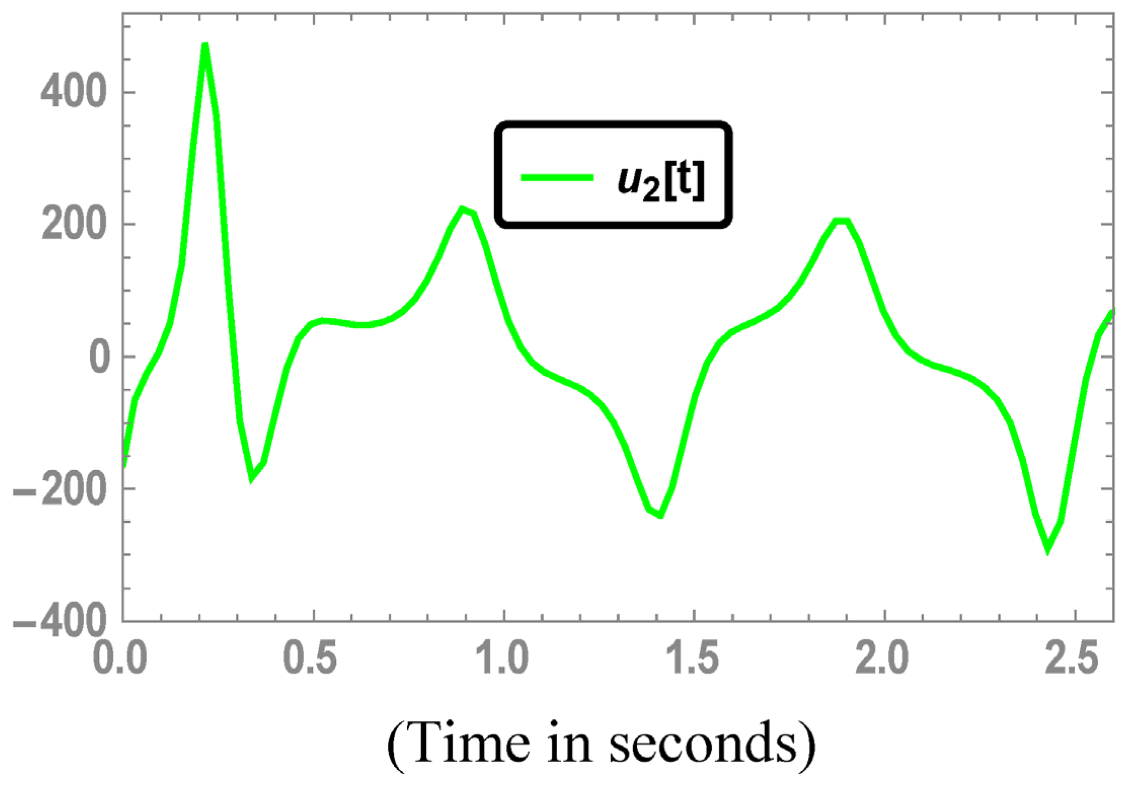
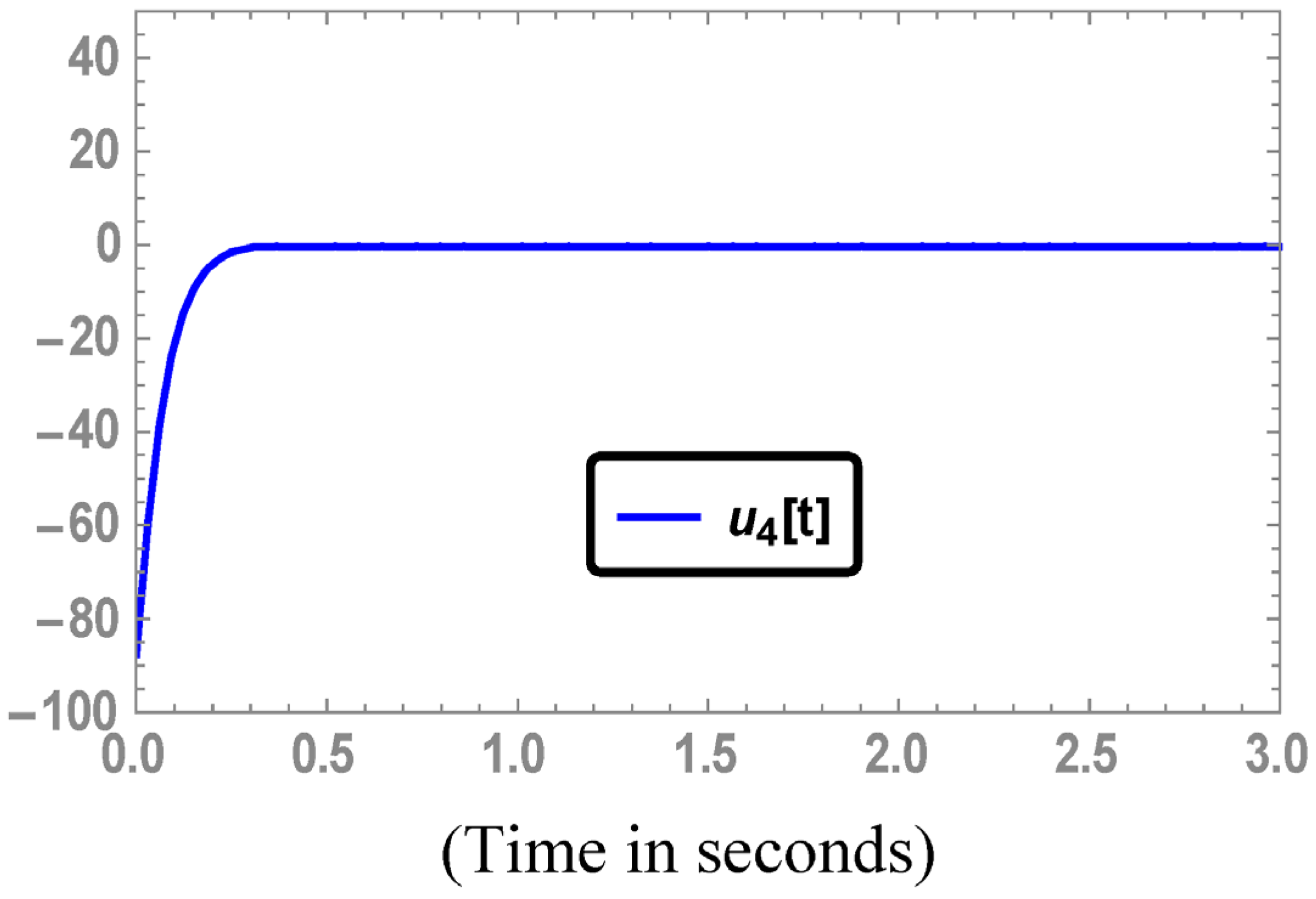
Figure 7.
Times series of the control input .
Figure 7.
Times series of the control input .
4. Finite-Time Increased Order Anti-Synchronization Scheme
4.1. Problem Statement
To achieve the finite-time increased order AS, the chaotic Lu system is considered as the master system and the hyperchaotic Li system as the slave system. Let us consider the following master-slave system increased order AS scheme between the chaotic Lu and the hyperchaotic Li systems as:
where
are the state variables,
and
are the control parameters of the master and slave systems alternatively.
and
are the unknown model uncertainties and external disturbances present in the master and slave systems respectively and
is the control input. The error system for the increased order AS scheme Equation (24) is described as follows:
Under these conditions, it is desired to design a controller that synthesis a smooth control input . This control inputs accomplishes the increased order AS within finite-time .
The increased order AS objectives are summarized as follows:
Objective 3. The increased order AS scheme is accomplished if:
Objective 4. The AS error dynamical system Equation (24) is globally stable in the finite time given by Equation (27).
4.2. Controller Design
Theorem 2. For the arbitrary initial conditions:
; of the master and slave systems respectively, the error system Equation (25) will converge to zero globally under the control law given by:
in the finite-time
, determined by:
Then, the objectives 3 and 4 are accomplished.
Proof of Theorem 2. Construct a Lyapunov function candidate as follows:
Now calculate the time derivatives of
along the trajectories of the error system Equation (25) that yields:
Now introducing the control inputs
Equation (26) to the right hand side of Equation (29) that yields:
Using Lemma 1, then, Equation (30) yields as follows:
where
are two positive constants. Let us choose
such that:
Using Equation (32), then, Equation (31)
Using Lemma 2, Equation (33) yields:
Using Lemma 3, yields the following inequality:
Hence, the closed-loop system Equation (25) is globally stable in the finite-time . This completes the proof.
4.3. Simulation and Results
The parameters and initial conditions for the hyperchaotic Li and chaotic Lu systems are selected in the same way as in Sub-
Section 3.3. The linear controller gains
are chosen as
and the constant number
being taken as
. In simulation, the following model uncertainties and external disturbances are applied to the master and slave systems respectively.
As a result, one can see that . The corresponding numerical results are as follows:
Time series of the increased order AS error signals is depicted in
Figure 8. As expected, one can observe that the AS error signals converged to zero state quickly with small amplitude of the oscillations.
Figure 9, shows the time series of the finite-time
Equation (27). From the main Theorem 2, it can be checked that the slave hyperchaotic Li system is anti-synchronized with the master chaotic Lu system under the control action Equation (26) in the finite-time, when the control inputs are activated at
. Times series of the control inputs are depicted in
Figure 10,
Figure 11,
Figure 12 and
Figure 13.
Figure 8.
Times series of the AS error signals.
Figure 8.
Times series of the AS error signals.
Figure 9.
Time series of the estimated finite time .
Figure 9.
Time series of the estimated finite time .
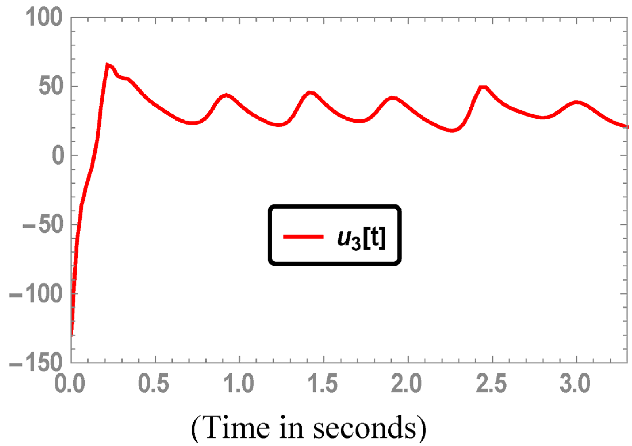
Figure 10.
Times series of the control input .
Figure 10.
Times series of the control input .
Figure 11.
Times series of the control input .
Figure 11.
Times series of the control input .
Figure 12.
Times series of the control input .
Figure 12.
Times series of the control input .
Figure 13.
Times series of the control input .
Figure 13.
Times series of the control input .
5. Conclusions
In this article, it has been established that the finite-time reduced order and increased order AS of chaotic systems can be accomplished. Sufficient conditions for the controller parameter design are derived. The closed-loop systems are then simulated and the anti-synchronization behavior is analyzed. The simulation results fully verify the analytical findings. The obtained results show that the proposed finite-time reduced order and increased order AS schemes are comparable with the published notable results in terms of AS speed and quality under the effect of both unknown model uncertainties and external disturbances. It has been confirmed that the reduced order and increased order AS error signals converged to the equilibrium point in the finite time with smaller amplitude of the oscillations.
In practical applications, it is difficult to exactly fix the values of the systems parameters in advance, which is a limitation of the proposed finite-time AS approach and will be addressed in our next research article or elsewhere.


