1. Introduction
The history of fractional calculus is almost as long as integer calculus, however it is only in the last few decades that it has gained much importance. The modeling of a variety of non-classic phenomena,
i.e., anomalous diffusion using fractional differential equations have proven to be promising to describe processes with memory and hereditary in geophysics [
1], physics [
2], chemistry [
3], biology [
4] and even finance and economics [
5]. The primary advantage of such modeling lies in the introduction of a parameter, namely the fractional order of the equation, which can be used to model non-Markovian behavior of spatial or temporal processes. While analytical methods, such as the Fourier transform method, the Laplace transform methods, and the Mellin transform method, have been developed to seek closed-form analytical solutions for fractional partial differential equations [
6], there are very few cases in which the closed-form analytical solutions are available, just like in the case of integer-order partial differential equations. Numerical methods for the fractional partial differential equations, such as finite difference methods [
7], finite element methods [
8,
9], spectral methods [
10], and discontinuous Galerkin methods [
11,
12] have recently been developed and remains a relatively new topic of research because of the difficulties encountered.
Due to the non-local nature of fractional differential operators, numerical methods for fractional diffusion equations [
9,
13,
14] raise numerical difficulties that were not encountered in the numerical methods for second-order diffusion equations. A significant obstacle that is the direct result of this non-local behavior is that these methods generate discrete systems with full or dense coefficient matrices. Meerschaert and Tadjeran [
15,
16] utilized a shifted Grünwald-Letnikov difference approximation to develop an implicit Euler finite difference method for space-fractional diffsuion equation in one-dimension. Further, they proved that the method is unconditionally stable and has first-order convergence in space and time. However, these methods were solved via Gaussian elimination, consequently
account of operations and
account of storage are required to solve a problem of size
N.
This work focuses on the development of a fast iterative finite difference method for the accurate and efficient solution of the one-dimensional space-fractional diffusion equation. The immense computational cost and storage requirement for the one-dimensional space fractional diffusion equation was broken down recently by the authors of [
17]. In [
17] they proved that the stiffness matrix of [
15,
16] can be decomposed as a sum of diagonal matrix multiplied by a Toepltiz matrix. They utilize this decomposition and applied an operator splitting technique to the one-dimensional space-fractional diffusion equation to develop a fast operator-splitting finite difference method for the space-fractional diffusion equation in one space dimension. However, this method has a computational work account of
per iteration and has a memory need of
per time step, due to the use of the banded coefficient matrix. While this is a vast improvement from the traditional methods solved via Gaussian elimination, there is room for improvement. In this paper the proposed method retains the same accuracy as the regular finite difference methods solved via Gaussian elimination and the resulting fast algorithm has a computational cost of
per iteration at each time step and a memory requirement of only
per time step.
The rest of this paper is organized as follows.
Section 2 outlines the space-fractional diffusion equation we attempt to solve and presents the corresponding Meerschaert-Tadjeran finite difference method.
Section 3, begins by discussing the impact of the significantly increased computational work and memory requirement of the traditional implicit finite difference method. Then we continue with the development of the fast conjugate gradient squared finite difference formulation. This section concludes by describing how to efficiently store the stiffness matrix and how to implement a fast matrix-vector multiplication to speed up the iterative scheme. Our work in this section establishes that the fast method has a computational work of
per iteration and a memory requirement of
per time step, while retaining the same accuracy as the traditional finite difference methods. This is followed by numerical experiments in
Section 4 and concluding remarks in
Section 5.
2. The Implicit Finite Difference Method for Time-Dependent Space Fractional Diffusion Equation
Fractional order partial differential equations are generalizations of classical partial differential equations. Fractional derivatives in space are used to model anomalous diffusion, where particles spread either faster or slower than the classical model predicts. When a fractional derivative of order α replaces the second derivative in a diffusion model, it leads to enhanced diffusion if (a process known as superdiffusion) or leads to subdiffusion, if .
For a one-dimensional fractional diffusion model with constant coefficients, analytic solutions are available [
18] using Fourier transform methods. However many practical problems require a model with variable coefficients [
19,
20]. In [
18], a space-fractional diffusion equation was used to describe Lévy flights.
We now proceed to develop a fast numerical method for space-fractional diffusion equations. Consider the following initial-boundary value problem of a class of time-dependent space-fractional diffusion of order
[
15,
16,
18]
The case
has useful applications [
21]. It is also a physically meaningful case, as explained in [
22]. A two-sided fractional partial differential equation allows modeling different flow regime impacts from either side. Here the left-sided (+) and the right-sided (−) fractional derivatives
and
can be defined in the (computationally feasible) Grünwald-Letnikov form [
23]
where
represents the floor of
x and
with
being the fractional binomial coefficients. We note that the Grünwald weights
can be evaluated using the recurrence relation
and satisfy the following properties [
15,
16,
23]
We also note that the left-handed fractional derivative of u at a point depends on all function values to the left of that point. Similarly, the right-handed fractional derivatives of u at a point depends on all function values to the right of this point. In other words, fractional derivatives are non-local operators.
This paper focuses on the development of a fast numerical method for problem Equation (
1). We refer to [
24], for the existence and uniqueness of the weak solution to fractional partial differential equations.
Let N and M be positive integers and and be the sizes of spatial grid and time step, respectively. We define a spatial and temporal partition for and for . Let , , , and .
We discertize the first-order time derivative in Equation (
1) by a standard first-order time difference quotient, but for the discretization of the fractional spatial derivative we use the shifted Grünwald approximations. Meerschaert and Tadjeran [
15,
16] showed that a fully implicit finite difference scheme with a direct truncation of the series in Equation (
2) turns out to be unstable! Using the following shifted Grünwald approximations
they proved that the corresponding implicit finite difference scheme
is unconditionally stable and convergent. Numerical experiments show that this scheme generates very satisfactory numerical approximations.
Let
,
,
, and
I be the identity matrix of order
. Then the numerical scheme Equation (
6) can be expressed in the following matrix form
Here the entries of matrix
are given by
It is clear that
for all
. We further conclude from Equations (
4) and (
8) that the coefficient matrix
is a nonsingular, strictly diagonally dominant M-matrix.
Equation (
8) implies that the scheme has a dense coefficient matrix, which has a memory requirement of
and computational work of
per time step. Thus the non-local nature of the fractional derivatives results in a full coefficient matrix of the system. This is in contrast to numerical methods for second-order diffusion equations which usually generate banded coefficient matrices of
nonzero entries and can be solved by fast solution methods such as multigrid methods, domain decomposition methods, and wavelet methods. Therefore the development of fast and robust numerical methods with efficient storage for the space-fractional diffusion equation is crucial for the applications of fractional diffusion equations.
3. The Fast Conjugate Gradient Squared Method
Since the stiffness matrix
is dense, solving Equation (
7) using Gaussian elimination requires computational work of
operations per iteration and memory storage of
per time step. For example, each time we reduce the size of the spatial mesh by half, the total number of unknowns per time step is doubled. As a result, the required memory increases 4 times, and the computational work increases 8 times. If the time step size is reduced by half too, then we would expect the overall consumed CPU time for solving the finite difference method to increases 16 times. Because of the significantly increased computational work and memory requirement of the numerical schemes for space-fractional diffusion equations, development of fast and reliable numerical methods with efficient storage mechanism has been of recent interest.
The goal of this paper is to develop a fast solution technique for the one-dimensional space-fractional diffusion equation via finite difference method Equation (
6). Let us begin by recalling the conjugate gradient squared iterative scheme to solve the system Equation (
7):
which can be expressed as follows
At each time step , we choose
Compute
Choose (for example, )
for
if the method fails
if
else
end if
Check for convergence; continue if necessary
end
Since the finite difference method has a nonsymmetric coefficient matrix in general, we need to use a nonsymmetric conjugate gradient method. Here we take the conjugate gradient squared method to solve the implicit Euler finite difference method Equation (
6).
Notice that in the above algorithm, at each time step
, the evaluation of the matrix-vector multiplication
,
and
costs
operations, while all others are already of optimal order computational cost
. Further, the storage of the stiffness matrix
requires
of memory, while all other operations require only
of memory. Our immediate goal is to develop a fast conjugate gradient squared method for the efficient solution and storage of the system Equation (
7).
In light of our goal, the rest of this section addresses the following important issues: (i) an efficient storage of the coefficient matrix with memory requirement of and (ii) how to perform an efficient matrix-vector multiplication with a general vector u in operations.
3.1. An Efficient Storage of the Stiffness Matrix
To develop a fast solution method with minimal memory requirement, we carefully explore the structure of the coefficient matrices.
Theorem 1. The total memory requirement for storing the coefficient matrix is .
Proof. We conclude from Equation (
8) that the stiffness matrix
can be decomposed as follows
Here
,
, are diagonal matrices of order
with their
ith entries
,
, for
. The matrices
and
are matrices of order
and are defined by
Thus, instead of storing the full matrix which have parameters we need only store the parameters, , , and . In particular, the fractional binomial coefficient vector depends only on the size of the spatial partition and the order of the anomalous diffusion but is independent of time or space. So it can be preprocessed and stored in advance. ☐
3.2. Toeplitz and Circulant Matrix
In order to explain the fast algorithm, we define the terms Toeplitz matrix and circulant matrix. A Toeplitz matrix is a matrix in which each descending diagonal from left to right is constant. Clearly, both matrices and are Toeplitz matrices. Also, is the transpose of .
A circulant matrix is a matrix in which each row vector is rotated one element to the right relative to the preceding row vector. It is clear that a circulant matrix is a Toeplitz matrix, but the converse is not true. Note that the Toeplitz matrices
and
can be embedded into
circulant matrices
and
as:
where
and
Again, note that
is the transpose of
.
It is known that a circulant matrix
can be decomposed as follows [
25,
26]
where
is the first column vector of
and
is the
discrete Fourier transform matrix in which the
-entry
of the matrix
is given by
where
.
We make use of the above decomposition property of circulant matrices to efficiently execute all matrix-vector multiplications , and of the conjugate gradient squared method above.
3.3. A Fast Matrix-Vector Multiplication Algorithm
We now shift our focus to the efficient operation of the numerical scheme. To efficiently execute the matrix-vector multiplications
,
and
of the conjugate gradient squared method, we use the following
algorithm, based on the decomposition Equation (
9) of the matrix
, the diagonalization Equation (
14) of a circulant matrix and the embedding Equation (
11).
Theorem 2. Let be the stiffness matrix as Equation (8). Let u be any N dimensional vector. Then can be performed in operations. Proof. We explain the operation count of
by executing the following steps:
Introduce two
matrices and one
vector
Here
and
are defined as in Equation (
12) and Equation (
13) and
and
as in Equation (
10) respectively. It is clear that
Thus, the matrix-vector products
and
can be obtained as the first half of the matrix-vector products
and
, respectively.
Evaluate the matrix-vector products in operations. In fact, is the discrete Fourier transform of , which can be achieved in operations via the fast Fourier transform (FFT).
Similarly evaluate and in operations, where and are the first column vectors of and , respectively.
Evaluate the Hadamard products and in operations.
Evaluate
and
in
operations via inverse FFT. Combining Equation (
16) and Equation (
17) yields that
Evaluate the Hadamard products
and
in
operations. Use Equation (
9) to evaluate
in
operations.
☐
4. Numerical Experiments
In this section we carry out numerical experiments to study the performance of the fast conjugate gradient squared finite difference method developed in this paper and to compare its performance with the finite difference methods with full coefficient matrices which were developed in [
15,
16].
We consider the fractional diffusion equation Equation (
1) with an anomalous diffusion of order
and the left-sided and right-sided diffusion coefficients
The spatial domain is
, the time interval is
. The source term and the initial condition are given by
The true solution to the corresponding fractional diffusion equation Equation (
1) is given by [
16]
In the numerical experiments, we solve the problem by both the fast conjugate squared (iterative) finite difference method and the regular finite difference method Equation (
6) and denote their solutions by
and
, respectively. Let
be the numerical solution
or
at time step
and
be the true solution to problem Equation (
1).
In
Table 1 we present the errors
and
for different spatial mesh sizes and time steps. These results are very encouraging and show that fast conjugate gradient squared finite difference method developed in this paper generates numerical solutions with same accuracy as the regular finite difference method, despite the fact that the former has significantly reduced the storage and computational cost of the latter from
and
to
and
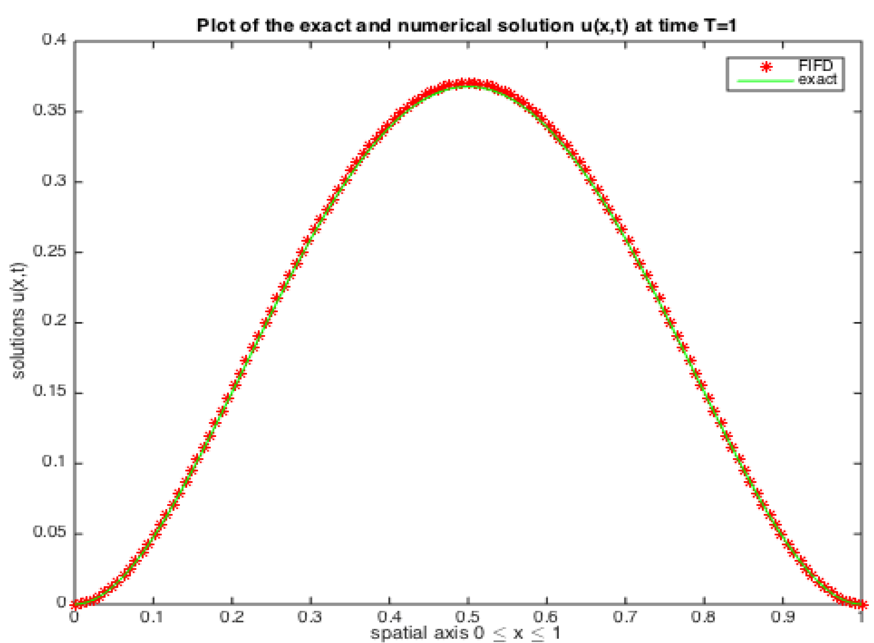
, respectively. We also present a representative plot with
in
Figure 1, which shows that the fast conjugate gradient squared finite difference solution and the regular finite difference solution both sit on the curve of the true solution without stark differences.
The numerical experiment carried out in this section shows the significant reduction in computational time which coincides with the theoretical analysis. For example, with nodes the fast conjugate gradient finite difference scheme developed in this paper has about 280 times of CPU reduction than the standard finite difference scheme solved with Gaussian elimination. This is on top of the significant reduction in storage. This demonstrates the strong potential of the method.
Table 1.
Comparison of the fast iterative finite difference (FIFD) method with the regular finite difference (FD) method in the simulation of the fractional diffusion problem with a known analytical solution.
Table 1.
Comparison of the fast iterative finite difference (FIFD) method with the regular finite difference (FD) method in the simulation of the fractional diffusion problem with a known analytical solution.
| | | ERROR | CPU (Seconds) |
|---|
| FD | | | |
| | |
| | |
| | |
| | | | |
| FIFD | | | |
| | |
| | |
| | |
| | | | |
Figure 1.
The true solution u (marked by “—”), the fast iterative finite difference solution (marked by “*”), in §4 at time with and .
Figure 1.
The true solution u (marked by “—”), the fast iterative finite difference solution (marked by “*”), in §4 at time with and .
5. Concluding Remarks and Future Work
This paper develops a fast solution method for the implicit finite difference scheme Equation (
6) for the one-dimensional space-fractional diffusion equation developed by Meerschaert and Tadjeran in [
15,
16]. The fast method consists of carefully analyzing the structure of the coefficient matrix resulting from the finite difference method, delicately decomposing the coefficient matrix into a combination of sparse and structured dense matrices and applying an iterative scheme, in this case the conjugate gradient squared method. Over the past decade many numerical methods have been developed for space-fractional diffusion equations, however all of them present major computational obstacles in realistic numerical simulation because of the significant computational cost and memory requirement. The fast conjugate gradient squared method developed in this paper keeps the same accuracy as the finite difference method [
15,
16] with Guassian elimination but has a memory requirement of only
per time step and a computational work of
per iteration.
Numerical computations were carried out using MATLAB. Furthermore, in order to use the fast conjugate gradient squared finite difference method, users need only rewrite a module to replace the matrix-vector multiplication module in traditional conjugate gradient method software. And this fast matrix-vector multiplication is based on FFT, which is readily available in MATLAB. Thus, the fast method virtually does not require any additional coding work to implement.
The idea of fast solution developed in this paper can be applied to other numerical methods. A fast solution method for a second-order Crank-Nicolson finite difference method was developed in [
27] for space-fractional diffusion equations in one dimension.
The reader should also note that a large diffusion coefficient could potentially lead to a large condition number of the coefficient matrix. This would in turn increase the number of iterations in the conjugate gradient squared method. Circulant preconditioners [
28,
29] and multigrid methods [
30] have been developed for some model problems which have shown significant improvements, under special conditions. The trade-off in forming and applying a preconditioner also needs to be examined. This can be an avenue for further research for this class of problems.


