A Variable Control Chart under the Truncated Life Test for a Weibull Distribution


1
Department of Statistics and Computer Science, University of Veterinary and Animal Sciences (UVAS), Lahore 54000, Pakistan
2
Department of Statistics, Faculty of Science, King Abdulaziz University, Jeddah 21551, Saudi Arabia
3
Department of Mathematics and Statistics, Riphah International University, Islamabad 44000, Pakistan
4
Department of Industrial and Management Engineering, Pohang University of Science and Technology (POSTECH), Pohang 37673, Korea
*
Author to whom correspondence should be addressed.
Technologies 2018, 6(2), 55; https://doi.org/10.3390/technologies6020055
Submission received: 9 May 2018
/
Revised: 25 May 2018
/
Accepted: 7 June 2018
/
Published: 10 June 2018
Abstract
:In this manuscript, a variable control chart under the time truncated life test for the Weibull distribution is presented. The procedure of the proposed control chart is given and its run length properties are derived for the shifted process. The control limit is determined by considering the target in-control average run length (ARL). The tables for ARLs are presented for industrial use according to various shift parameters and shape parameters in the Weibull distribution. A simulation study is given for demonstrating the performance of the proposed control chart.
1. Introduction
A control chart is considered a powerful tool for maintaining the high quality of products in industry. This tool is used to monitor the industrial process from raw material to final product. The process can shift from the target value due to several extraneous factors. The control chart should provide a quick indication about a shift in a manufacturing process, if there is any. This quick indication helps the industrial engineer to look at the problem and bring it back into control state.
Two types of control charts are widely used in the industry for monitoring the manufacturing process. Attribute control charts are used when the data is coming from the counting process and variable control charts are used when the data is obtained from the measurement process. The attribute control charts are easy to apply but the variable control charts are more informative than attribute charts. Usually, variables control charts are developed under the assumption that the characteristic follows the normal distribution.
In practice, a control chart designed for normal distribution may not be effective for monitoring the manufacturing process when the characteristic of interest does not follow the normal distribution. The use of this type of control chart may lead to a wrong decision about the status of the manufacturing state. Derya and Canan [1] mentioned that “the distributions of measurements in chemical processes, semiconductor processes, cutting tool wear processes and observations on lifetimes in accelerated life test samples are often skewed”. Several authors focused on this issue and designed control charts for non-normal data. Al-Oraini and Rahim [2] designed a control chart for a gamma distribution. Amin et al. [3] designed a non-parametric chart using a sign statistic. Chang and Bai [4] worked for a control chart for a positive skewed population, Chen and Yeh [5] worked for an economical statistical design of a control chart for a gamma distribution. McCracken and Chakraborti [6] presented a control chart for monitoring mean and variance for a normal distribution. Yen et al. [7] designed a Synthetic-type contro for time between events. Riaz et al. [8] proposed a median control chart and Abujiya et al. [9] worked for the cumulative sum control chart (CUSUM) control chart. Gonzalez and Viles [10] designed a R chart using gamma distribution, Lio and Park [11] designed a control chart for inverse Gaussian percentiles. Huang and Pascual [12] designed a control chart for Weibull percentiles using the order statistic. Derya and Canan [1] designed the control charts for the Weibull distribution, gamma distribution, and log-normal distribution and [13] proposed a control chart for the Burr type X distribution. Aslam et al. [14] deigned control chart for the exponential distribution using exponentially weighted moving average (EWMA) statistic.
For the reliability evaluation of a product, the time truncated life test is often adopted in industries for saving the experiment time. Therefore, the designing of a control chart under the time truncated test is important when monitoring the process in terms of reliability. Aslam et al. [15] proposed an attribute control chart under the time truncated life test by assuming that the failure time of a product follows the Weibull distribution. Aslam et al. [16] designed a time truncated attribute control chart using the Pareto distribution. Aslam et al. [17] deigned a time truncated control chart for the Birnbaum-Saunders distribution under repetitive sampling. More details about such control charts can be read in Aslam et al. [18], Arif et al. [19], Khan et al. [20], and Shafqat et al. [21].
In summary, control charts under the time truncated life test for various situations or distributions are available for the attribute quality of interest. However, these control charts cannot be applied for the monitoring of a measurable quality of interest. From exploring the literature and from the best of our knowledge, there is no work on the design of a variable control chart under the time truncated life test. In this paper, we will propose a variable control chart for a Weibull distribution using failure data from a time truncated life test. A real example is given for illustration purposes and a simulation study is added to demonstrate the performance of the proposed control chart.
2. Proposed Chart and Its Average Run Length (ARLs)
The assumptions of the proposed control chart are stated as follows:
- It is assumed that the quality characteristic of interest follows a Weibull distribution.
- The shape parameter of the Weibull distribution is assumed to be known.
- When the process is shifted, the scale parameter is changed to , where is a shift constant and is the scale parameter for the in-control process. The shape parameter remains unchanged when the process is shifted.
- Failure times are measured during the time truncated life test.
Let the variable of interest follow the Weibull distribution with the cumulative distribution function (cdf) of:
where is the shape parameter and is the scale parameter. The average life time, of the variable is given by:
where is a gamma function.
The proposed control chart is operated as follows:
- Step 1
- Take a sample of size at each subgroup from the production process. Put them on test until the specified time .
- Step 2
- Obtain the time to failure of item i (denoted by ). Set if item i does not fail by time . Calculate statistics .
- Step 3
- Obtain , is average of . Declare the process as in-control if or as out-of-control if , where represents the control limit.
2.1. Distribution of Control Statistics and In-Control Average Run Length (ARL)
To derive the necessary measures of average run length (ARL), it would be convenient to select the specified time , as a fraction of the mean for the in control process, where is a constant and is the target mean.
As the transformed variable is modeled to an exponential distribution with mean , the sum of Y’s (or ) follows a gamma distribution. But, the distribution of approximately follows a normal distribution according to the central limit theorem, as long as the sample size is sufficient. Then, the expected value of can be obtained by:
Here, is obtained by:
Equation (4) reduces to:
The variance of is given as follows:
The simplified form of can be rewritten as:
Let be the probability of being declared as in control when the process is actually in control at . Then, it is given as follows:
Finally, can be written as follows:
The efficiency of the proposed chart will be measured through the ARL, which shows when the process will be out-of-control. Let be the ARL for in control process. Then, it is given as follows:
2.2. Out of Control ARL
Let us assume that the process has shifted due to some factors to a new scale parameter , where is the shift constant. Now, we derive the measures for the shifted process. Let be the probability of declaring the state of being in control when the process has shifted to , which is given as follows:
The distribution of at approximately follows normal with the mean and the variance given below:
Therefore, the in-control probability for the shifted process, say in Equation (11), is obtained by:
Hence, the out-of-control ARL, say for the shifted process is given as follows:
The values of for the various values of the shape parameters, , and, , are presented in Table 1, Table 2, Table 3, Table 4, Table 5, Table 6, Table 7 and Table 8. Let be the specified in-control ARL. The control limit is determined by using the following algorithm:
- Prefix the value of .
- The value is obtained such that .
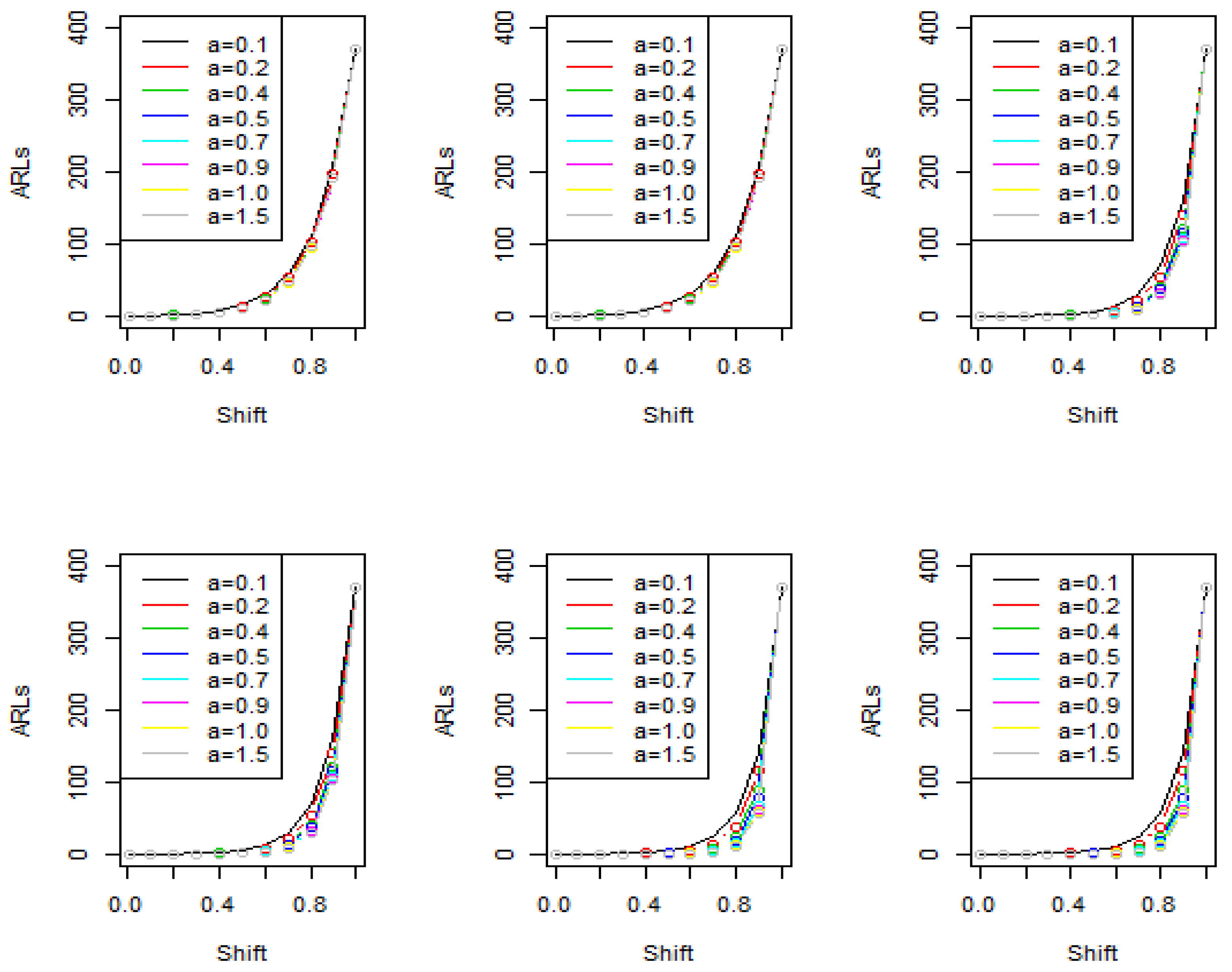
From Table 1, Table 2, Table 3, Table 4, Table 5, Table 6, Table 7 and Table 8 and Figure 1, we note the following trends in .
- As increases, we note to decrease for the same shift in process. This seems reasonable because the number of failures observed increases as increases.
- For a fixed , as decreases, also decreases because the true mean time to a failure decreases.
- For other fixed parameters, as increases from 50 to 100, the behavior of remains quite similarly, which is a desirable feature.
- For other fixed parameters, as increases from 0.5 to 2, decreases.
3. Simulation Study
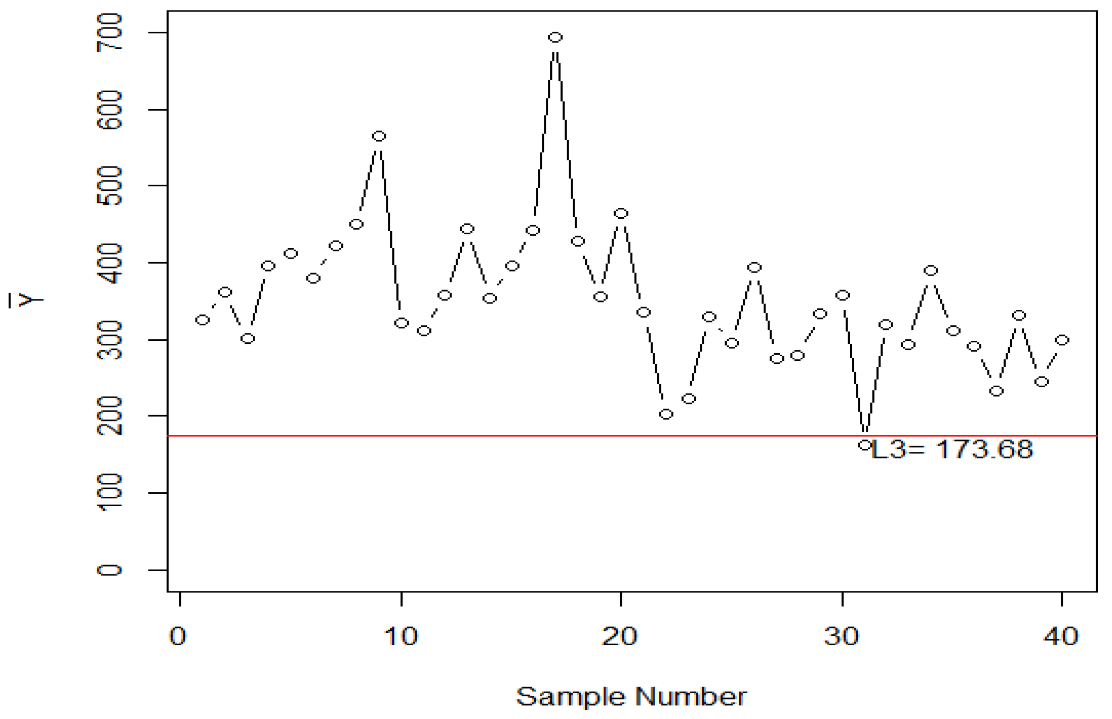
In this section, we discuss the performance of the proposed control chart using simulated data. The data is generated from the Weibull distribution with the shape parameters and . The first 20 observations are generated from an in-control process and the next 20 observations are generated from a shifted process with .
We applied this data to the proposed control chart having and = 370. The control limit L3 is obtained by 173.68. The values of are calculated and plotted on the control chart. From Figure 2, we note that the proposed chart detects the shift in the process at the 31st sample.
4. Real Example
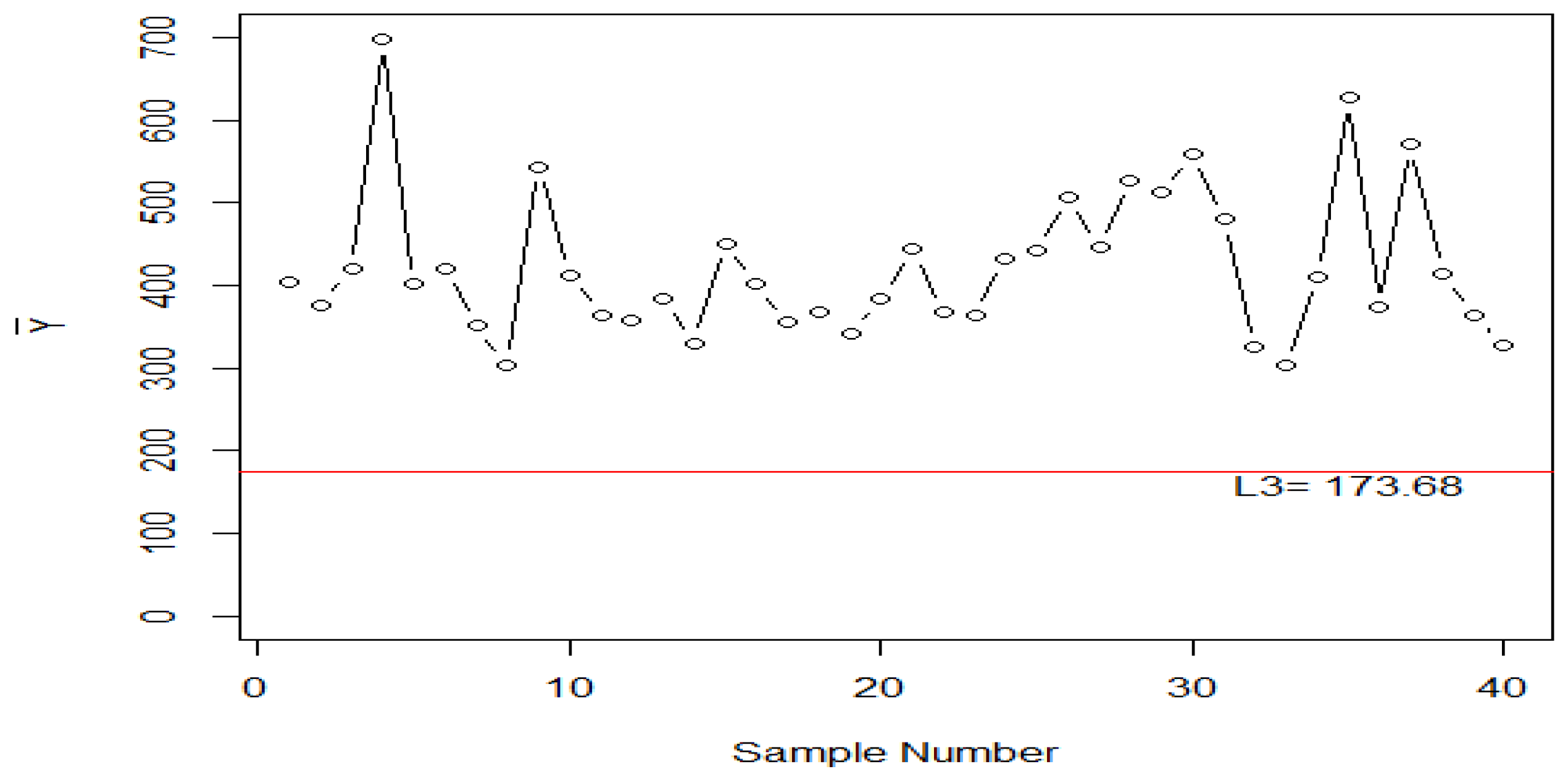
In this section, we will discuss the application of the proposed control chart using the breaking stress data of carbon fibers from an industry. Carbon fiber has good tensile strength, which is measured in force per unit area (GPa). For more details, see Yu et al. [22]. The carbon fibers data given in GPa is modeled by the Weibull distribution when = 1. For this study, let = 30 and = 370. The values of statistic for this data are shown below:
- 404, 377, 420, 698, 402, 421, 352, 303, 544, 413, 365, 359, 383, 330, 451, 402, 355, 368, 342, 383, 444, 368, 364, 433, 443, 508, 447, 528, 512, 559, 481, 325, 303, 410, 628, 373, 571, 414, 364, 328.
By plotting on a control chart, Figure 3 shows that the process is in control but some points are close to the lower control limit.
5. Conclusions
In this paper, a new variable chart under the truncated life test is designed for the Weibull distribution. The average run length is derived to measure the efficiency of the proposed chart. Extensive tables are given for industrial use. The application of the proposed chart is given with the help of simulation data. The proposed chart is sensitive in detecting the shift in the process. The proposed control chart can be used in a real industry where the lifetime of the product follows the Weibull distribution. The proposed chart using unknown shape parameters can be a fruitful future research.
Author Contributions
Conceptualization, N.K., M.A., M.Z.K. and C.H.J.; Methodology, N.K., M.A., M.Z.K. and C.H.J.; Software, N.K., M.A., M.Z.K. and C.H.J.; Validation, N.K., M.A., M.Z.K. and C.H.J; Formal Analysis, N.K., M.A., M.Z.K. and C.H.J.; Writing-Original Draft Preparation, M.A., and C.H.J.; Writing-Review & Editing, N.K., M.A., M.Z.K. and C.H.J.
Funding
This research received no external funding.
Acknowledgments
The authors are deeply thankful to the editor and the reviewers for their valuable suggestions to improve the quality of this manuscript. This article was funded by the Deanship of Scientific Research (DSR) at King Abdulaziz University, Jeddah. The author, Muhammad Aslam, therefore, acknowledge with thanks DSR technical and financial support.
Conflicts of Interest
The authors declare no conflict of interest.
References
- Derya, K.; Canan, H. Control Charts for Skewed Distributions: Weibull, Gamma, and Lognormal. Metodoloski Zvezki 2012, 9, 95–106. [Google Scholar]
- Al-Oraini, H.A.; Rahim, M. Economic statistical design of X control charts for systems with Gamma (λ, 2) in-control times. Comput. Ind. Eng. 2002, 43, 645–654. [Google Scholar] [CrossRef]
- Amin, R.W.; Reynolds, M.R., Jr.; Saad, B. Nonparametric quality control charts based on the sign statistic. Commun. Stat.-Theor. Methods 1995, 24, 1597–1623. [Google Scholar] [CrossRef]
- Chang, Y.S.; Bai, D.S. Control charts for positively-skewed populations with weighted standard deviations. Qual. Reliab. Eng. Int. 2001, 17, 397–406. [Google Scholar] [CrossRef]
- Chen, F.; Yeh, C. Economic statistical design of non-uniform sampling scheme X bar control charts under non-normality and Gamma shock using genetic algorithm. Expert Syst. Appl. 2009, 36, 9488–9497. [Google Scholar] [CrossRef]
- McCracken, A.; Chakraborti, S. Control charts for joint monitoring of mean and variance: An overview. Qual. Technol. Quant. Manag. 2013, 10, 17–35. [Google Scholar] [CrossRef]
- Yen, F.Y.; Chong, K.M.B.; Ha, L.M. Synthetic-type control charts for time-between-events monitoring. PLoS ONE 2013, 8, e65440. [Google Scholar] [CrossRef] [PubMed]
- Ahmad, S.; Riaz, M.; Abbasi, S.A.; Lin, Z. On efficient median control charting. J. Chin. Inst. Eng. 2014, 37, 358–375. [Google Scholar] [CrossRef]
- Abujiya, M.R.; Riaz, M.; Lee, M.H. Enhanced Cumulative Sum Charts for Monitoring Process Dispersion. PLoS ONE 2015, 10, e0124520. [Google Scholar] [CrossRef] [PubMed]
- Gonzalez, I.M.; Viles, E. Design of R control chart assuming a gamma distribution. Econ. Qual. Control 2001, 16, 199–204. [Google Scholar] [CrossRef]
- Lio, Y.; Park, C. A bootstrap control chart for inverse Gaussian percentiles. J. Stat. Comput. Simul. 2010, 80, 287–299. [Google Scholar] [CrossRef]
- Huang, X.; Pascual, F. ARL-unbiased control charts with alarm and warning lines for monitoring Weibull percentiles using the first-order statistic. J. Stat. Comput. Simul. 2011, 81, 1677–1696. [Google Scholar] [CrossRef]
- Lio, Y.L.; Tsai, T.-R.; Aslam, M.; Jiang, N. Control charts for monitoring Burr type-X percentiles. Commun. Stat.-Simul. Comput. 2014, 43, 761–776. [Google Scholar] [CrossRef]
- Aslam, M.; Azam, M.; Jun, C.-H. A new control chart for exponential distributed life using EWMA. Trans. Inst. Meas. Control 2015, 37, 205–210. [Google Scholar] [CrossRef]
- Aslam, M.; Jun, C.-H. Attribute Control Charts for the Weibull Distribution under Truncated Life Tests. Qual. Eng. 2015, 27, 283–288. [Google Scholar] [CrossRef]
- Aslam, M.; Khan, N.; Jun, C.-H. A control chart for time truncated life tests using Pareto distribution of second kind. J. Stat. Comput. Simul. 2016, 86, 2113–2122. [Google Scholar] [CrossRef]
- Aslam, M.; Arif, O.H.; Jun, C.-H. An Attribute Control Chart Based on the Birnbaum-Saunders Distribution Using Repetitive Sampling. In IEEE Access; IEEE: Washington, DC, USA, 2016. [Google Scholar]
- Aslam, M.; Arif, O.H.; Jun, C.-H. An attribute control chart for a Weibull distribution under accelerated hybrid censoring. PLoS ONE 2017, 12, e0173406. [Google Scholar] [CrossRef] [PubMed]
- Arif, O.-H.; Aslam, M.; Jun, C.-H. EWMA np Control Chart for the Weibull Distribution. J. Test. Eval. 2016, 45, 1022–1028. [Google Scholar] [CrossRef]
- Khan, N.; Aslam, M.; Kim, K.-J.; Jun, C.-H. A mixed control chart adapted to the truncated life test based on the Weibull distribution. Oper. Res. Decis. 2017, 27, 43–55. [Google Scholar]
- Shafqat, A.; Hussain, J.; Al-Nasser, A.D.; Aslam, M. Attribute control chart for some popular distributions. Commun. Stat.-Theor. Methods 2018, 47, 1978–1988. [Google Scholar] [CrossRef]
- Yu, M.F.; Lourie, O.; Dyer, M.J.; Moloni, K.; Kelly, T.F.; Ruoff, R.S. Strength and breaking mechanism of multiwalled carbon nanotubes under tensile load. Science 2000, 287, 637–640. [Google Scholar] [CrossRef] [PubMed]
Figure 1.
The average run length (ARLs) curves.

Figure 2.
The proposed chart using simulated data.

Figure 3.
Proposed chart for the carbon fibers data.


Table 1.
The values of ARLs when , .
| 0.1 | 0.2 | 0.4 | 0.5 | 0.7 | 0.9 | 1 | 1.5 | |
| L | 1.45 | 1.80 | 2.15 | 2.25 | 2.39 | 2.47 | 2.51 | 2.60 |
| c | ARL1 | |||||||
| 1 | 371.89 | 370.16 | 370.03 | 370.20 | 370.32 | 370.00 | 370.15 | 370.37 |
| 0.9 | 206.44 | 198.53 | 193.29 | 192.28 | 191.36 | 191.09 | 191.28 | 192.92 |
| 0.8 | 111.78 | 103.82 | 98.36 | 97.24 | 96.19 | 95.91 | 96.03 | 97.43 |
| 0.7 | 58.89 | 52.83 | 48.67 | 47.80 | 46.94 | 46.69 | 46.72 | 47.57 |
| 0.6 | 30.11 | 26.12 | 23.40 | 22.82 | 22.23 | 22.02 | 22.01 | 22.41 |
| 0.5 | 14.92 | 12.56 | 10.96 | 10.61 | 10.24 | 10.09 | 10.07 | 10.20 |
| 0.4 | 7.18 | 5.90 | 5.05 | 4.86 | 4.65 | 4.56 | 4.54 | 4.55 |
| 0.3 | 3.40 | 2.78 | 2.38 | 2.28 | 2.18 | 2.12 | 2.11 | 2.09 |
| 0.2 | 1.67 | 1.43 | 1.27 | 1.24 | 1.20 | 1.18 | 1.17 | 1.16 |
| 0.1 | 1.04 | 1.01 | 1.00 | 1.00 | 1.00 | 1.00 | 1.00 | 1.00 |
Table 2.
The values of ARLs when .
| a | ||||||||
| 0.1 | 0.2 | 0.4 | 0.5 | 0.7 | 0.9 | 1 | 1.5 | |
| L | 2.05 | 2.55 | 3.04 | 3.18 | 3.38 | 3.50 | 3.54 | 3.68 |
| c | ARL1 | |||||||
| 1 | 370.08 | 370.09 | 370.40 | 370.05 | 370.20 | 370.03 | 370.04 | 370.04 |
| 0.9 | 205.51 | 198.49 | 193.48 | 192.21 | 191.31 | 191.10 | 191.23 | 192.75 |
| 0.8 | 111.32 | 103.81 | 98.45 | 97.21 | 96.16 | 95.92 | 96.00 | 97.35 |
| 0.7 | 58.67 | 52.82 | 48.71 | 47.78 | 46.93 | 46.69 | 46.71 | 47.53 |
| 0.6 | 30.02 | 26.12 | 23.42 | 22.81 | 22.22 | 22.02 | 22.01 | 22.39 |
| 0.5 | 14.88 | 12.55 | 10.97 | 10.61 | 10.24 | 10.09 | 10.07 | 10.20 |
| 0.4 | 7.16 | 5.90 | 5.05 | 4.86 | 4.65 | 4.56 | 4.53 | 4.55 |
| 0.3 | 3.39 | 2.78 | 2.38 | 2.28 | 2.18 | 2.12 | 2.11 | 2.09 |
| 0.2 | 1.67 | 1.43 | 1.27 | 1.24 | 1.20 | 1.18 | 1.17 | 1.16 |
| 0.1 | 1.04 | 1.01 | 1.00 | 1.00 | 1.00 | 1.00 | 1.00 | 1.00 |
Table 3.
The values of ARLs when and .
| 0.1 | 0.2 | 0.4 | 0.5 | 0.7 | 0.9 | 1 | 1.5 | |
| l3 | 4.32 | 7.88 | 13.44 | 15.61 | 19.05 | 21.53 | 22.49 | 25.39 |
| c | ARL1 | |||||||
| 1 | 370.49 | 370.04 | 370.05 | 370.04 | 370.02 | 370.02 | 370.00 | 370.03 |
| 0.9 | 160.24 | 140.34 | 121.26 | 115.86 | 109.00 | 105.29 | 104.19 | 103.22 |
| 0.8 | 69.80 | 54.24 | 41.14 | 37.75 | 33.62 | 31.43 | 30.77 | 29.92 |
| 0.7 | 30.74 | 21.55 | 14.70 | 13.06 | 11.14 | 10.13 | 9.81 | 9.30 |
| 0.6 | 13.78 | 8.94 | 5.69 | 4.97 | 4.14 | 3.71 | 3.57 | 3.30 |
| 0.5 | 6.36 | 3.97 | 2.51 | 2.21 | 1.86 | 1.69 | 1.63 | 1.50 |
| 0.4 | 3.10 | 1.98 | 1.38 | 1.26 | 1.14 | 1.09 | 1.07 | 1.04 |
| 0.3 | 1.67 | 1.22 | 1.03 | 1.02 | 1.00 | 1.00 | 1.00 | 1.00 |
| 0.2 | 1.11 | 1.01 | 1.00 | 1.00 | 1.00 | 1.00 | 1.00 | 1.00 |
| 0.1 | 1.00 | 1.00 | 1.00 | 1.00 | 1.00 | 1.00 | 1.00 | 1.00 |
Table 4.
The values of ARLs when .
| a | ||||||||
| 0.1 | 0.2 | 0.4 | 0.5 | 0.7 | 0.9 | 1 | 1.5 | |
| l3 | 8.63 | 15.75 | 26.87 | 31.22 | 38.09 | 43.05 | 44.98 | 50.77 |
| c | ARL1 | |||||||
| 1 | 370.11 | 370.15 | 370.00 | 370.00 | 370.02 | 370.01 | 370.01 | 370.01 |
| 0.9 | 160.10 | 140.38 | 121.25 | 115.85 | 109.00 | 105.29 | 104.19 | 103.21 |
| 0.8 | 69.75 | 54.25 | 41.14 | 37.75 | 33.62 | 31.43 | 30.77 | 29.92 |
| 0.7 | 30.72 | 21.55 | 14.70 | 13.06 | 11.14 | 10.13 | 9.81 | 9.30 |
| 0.6 | 13.77 | 8.94 | 5.69 | 4.97 | 4.14 | 3.71 | 3.57 | 3.30 |
| 0.5 | 6.36 | 3.97 | 2.51 | 2.21 | 1.86 | 1.69 | 1.63 | 1.50 |
| 0.4 | 3.10 | 1.98 | 1.37 | 1.26 | 1.14 | 1.09 | 1.07 | 1.04 |
| 0.3 | 1.67 | 1.22 | 1.03 | 1.02 | 1.00 | 1.00 | 1.00 | 1.00 |
| 0.2 | 1.11 | 1.01 | 1.00 | 1.00 | 1.00 | 1.00 | 1.00 | 1.00 |
| 0.1 | 1.00 | 1.00 | 1.00 | 1.00 | 1.00 | 1.00 | 1.00 | 1.00 |
Table 5.
The values of ARLs when and .
| 0.1 | 0.2 | 0.4 | 0.5 | 0.7 | 0.9 | 1 | 1.5 | |
| l3 | 10.50 | 27.97 | 69.43 | 90.44 | 129.08 | 160.79 | 173.68 | 211.26 |
| c | ARL1 | |||||||
| 1 | 370.72 | 370.42 | 370.06 | 370.00 | 370.02 | 370.08 | 370.05 | 370.01 |
| 0.9 | 141.52 | 116.13 | 88.08 | 79.62 | 68.53 | 62.25 | 60.30 | 58.10 |
| 0.8 | 56.58 | 39.16 | 23.78 | 19.89 | 15.29 | 12.91 | 12.18 | 11.10 |
| 0.7 | 23.78 | 14.36 | 7.50 | 6.00 | 4.36 | 3.56 | 3.32 | 2.88 |
| 0.6 | 10.57 | 5.83 | 2.89 | 2.33 | 1.74 | 1.48 | 1.40 | 1.25 |
| 0.5 | 5.01 | 2.70 | 1.47 | 1.27 | 1.09 | 1.03 | 1.02 | 1.00 |
| 0.4 | 2.58 | 1.50 | 1.06 | 1.02 | 1.00 | 1.00 | 1.00 | 1.00 |
| 0.3 | 1.50 | 1.07 | 1.00 | 1.00 | 1.00 | 1.00 | 1.00 | 1.00 |
| 0.2 | 1.07 | 1.00 | 1.00 | 1.00 | 1.00 | 1.00 | 1.00 | 1.00 |
| 0.1 | 1.00 | 1.00 | 1.00 | 1.00 | 1.00 | 1.00 | 1.00 | 1.00 |
| 0 | 1.00 | 1.00 | 1.00 | 1.00 | 1.00 | 1.00 | 1.00 | 1.00 |
Table 6.
The values of ARLs when and .
| 0.1 | 0.2 | 0.4 | 0.5 | 0.7 | 0.9 | 1 | 1.5 | |
| l3 | 29.69 | 79.11 | 196.38 | 255.81 | 365.10 | 454.78 | 491.26 | 597.52 |
| c | ARL1 | |||||||
| 1 | 370.53 | 370.08 | 370.17 | 370.00 | 370.00 | 370.00 | 370.01 | 370.00 |
| 0.9 | 141.46 | 116.05 | 88.10 | 79.61 | 68.52 | 62.24 | 60.30 | 58.10 |
| 0.8 | 56.56 | 39.14 | 23.78 | 19.89 | 15.29 | 12.90 | 12.18 | 11.10 |
| 0.7 | 23.78 | 14.35 | 7.50 | 6.00 | 4.36 | 3.56 | 3.32 | 2.88 |
| 0.6 | 10.57 | 5.83 | 2.89 | 2.33 | 1.74 | 1.48 | 1.40 | 1.25 |
| 0.5 | 5.01 | 2.70 | 1.47 | 1.27 | 1.09 | 1.03 | 1.02 | 1.00 |
| 0.4 | 2.58 | 1.50 | 1.06 | 1.02 | 1.00 | 1.00 | 1.00 | 1.00 |
| 0.3 | 1.50 | 1.07 | 1.00 | 1.00 | 1.00 | 1.00 | 1.00 | 1.00 |
| 0.2 | 1.07 | 1.00 | 1.00 | 1.00 | 1.00 | 1.00 | 1.00 | 1.00 |
| 0.1 | 1.00 | 1.00 | 1.00 | 1.00 | 1.00 | 1.00 | 1.00 | 1.00 |
Table 7.
The values of ARLs when .
| 0.1 | 0.2 | 0.4 | 0.5 | 0.7 | 0.9 | 1 | 1.5 | |
| l3 | 24.25 | 93.32 | 336.83 | 493.78 | 832.31 | 1150.16 | 1286.31 | 1659.85 |
| c | ARL1 | |||||||
| 1 | 389.83 | 373.30 | 370.04 | 370.08 | 370.04 | 370.02 | 370.03 | 370.01 |
| 0.9 | 133.38 | 103.35 | 70.29 | 60.00 | 46.42 | 38.84 | 36.53 | 34.42 |
| 0.8 | 50.14 | 32.53 | 16.66 | 12.77 | 8.41 | 6.33 | 5.73 | 4.93 |
| 0.7 | 20.67 | 11.69 | 5.06 | 3.73 | 2.39 | 1.82 | 1.67 | 1.41 |
| 0.6 | 9.34 | 4.83 | 2.06 | 1.60 | 1.19 | 1.06 | 1.03 | 1.00 |
| 0.5 | 4.62 | 2.34 | 1.20 | 1.07 | 1.00 | 1.00 | 1.00 | 1.00 |
| 0.4 | 2.50 | 1.38 | 1.01 | 1.00 | 1.00 | 1.00 | 1.00 | 1.00 |
| 0.3 | 1.51 | 1.05 | 1.00 | 1.00 | 1.00 | 1.00 | 1.00 | 1.00 |
| 0.2 | 1.08 | 1.00 | 1.00 | 1.00 | 1.00 | 1.00 | 1.00 | 1.00 |
| 0.1 | 1.00 | 1.00 | 1.00 | 1.00 | 1.00 | 1.00 | 1.00 | 1.00 |
Table 8.
The values of ARLs when .
| r0 = 370; β = 1.5; u0 = 100 | ||||||||
| a | ||||||||
| 0.1 | 0.2 | 0.4 | 0.5 | 0.7 | 0.9 | 1 | 1.5 | |
| l3 | 97.02 | 373.31 | 1347.30 | 1975.12 | 3329.23 | 4600.66 | 5145.24 | 6639.42 |
| c | ARL1 | |||||||
| 1 | 373.80 | 370.47 | 370.01 | 370.06 | 370.01 | 370.01 | 370.01 | 370.00 |
| 0.9 | 128.96 | 102.73 | 70.29 | 59.99 | 46.42 | 38.84 | 36.53 | 34.42 |
| 0.8 | 48.83 | 32.38 | 16.66 | 12.77 | 8.41 | 6.33 | 5.73 | 4.93 |
| 0.7 | 20.27 | 11.65 | 5.06 | 3.73 | 2.39 | 1.82 | 1.67 | 1.41 |
| 0.6 | 9.21 | 4.82 | 2.06 | 1.60 | 1.19 | 1.06 | 1.03 | 1.00 |
| 0.5 | 4.57 | 2.34 | 1.20 | 1.07 | 1.00 | 1.00 | 1.00 | 1.00 |
| 0.4 | 2.49 | 1.38 | 1.01 | 1.00 | 1.00 | 1.00 | 1.00 | 1.00 |
| 0.3 | 1.51 | 1.05 | 1.00 | 1.00 | 1.00 | 1.00 | 1.00 | 1.00 |
| 0.2 | 1.08 | 1.00 | 1.00 | 1.00 | 1.00 | 1.00 | 1.00 | 1.00 |
| 0.1 | 1.00 | 1.00 | 1.00 | 1.00 | 1.00 | 1.00 | 1.00 | 1.00 |
© 2018 by the authors. Licensee MDPI, Basel, Switzerland. This article is an open access article distributed under the terms and conditions of the Creative Commons Attribution (CC BY) license (http://creativecommons.org/licenses/by/4.0/).
Share and Cite
MDPI and ACS Style
Khan, N.; Aslam, M.; Khan, M.Z.; Jun, C.-H. A Variable Control Chart under the Truncated Life Test for a Weibull Distribution. Technologies 2018, 6, 55. https://doi.org/10.3390/technologies6020055
AMA Style
Khan N, Aslam M, Khan MZ, Jun C-H. A Variable Control Chart under the Truncated Life Test for a Weibull Distribution. Technologies. 2018; 6(2):55. https://doi.org/10.3390/technologies6020055
Chicago/Turabian StyleKhan, Nasrullah, Muhammad Aslam, Muhammad Zahir Khan, and Chi-Hyuck Jun. 2018. "A Variable Control Chart under the Truncated Life Test for a Weibull Distribution" Technologies 6, no. 2: 55. https://doi.org/10.3390/technologies6020055
Note that from the first issue of 2016, this journal uses article numbers instead of page numbers. See further details here.