
An Experimental/Numerical Study on the Interfacial Damage of Bonded Joints for Fibre-Reinforced Polymer Profiles at Service Conditions


Abstract
:
1. Introduction
- -
- -
- -
2. Materials and Methods under Consideration
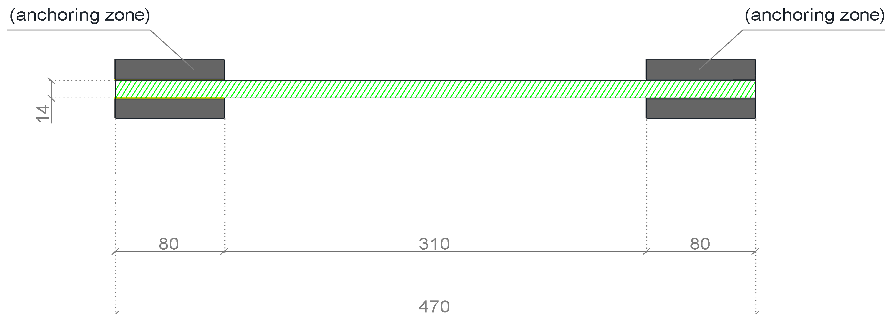
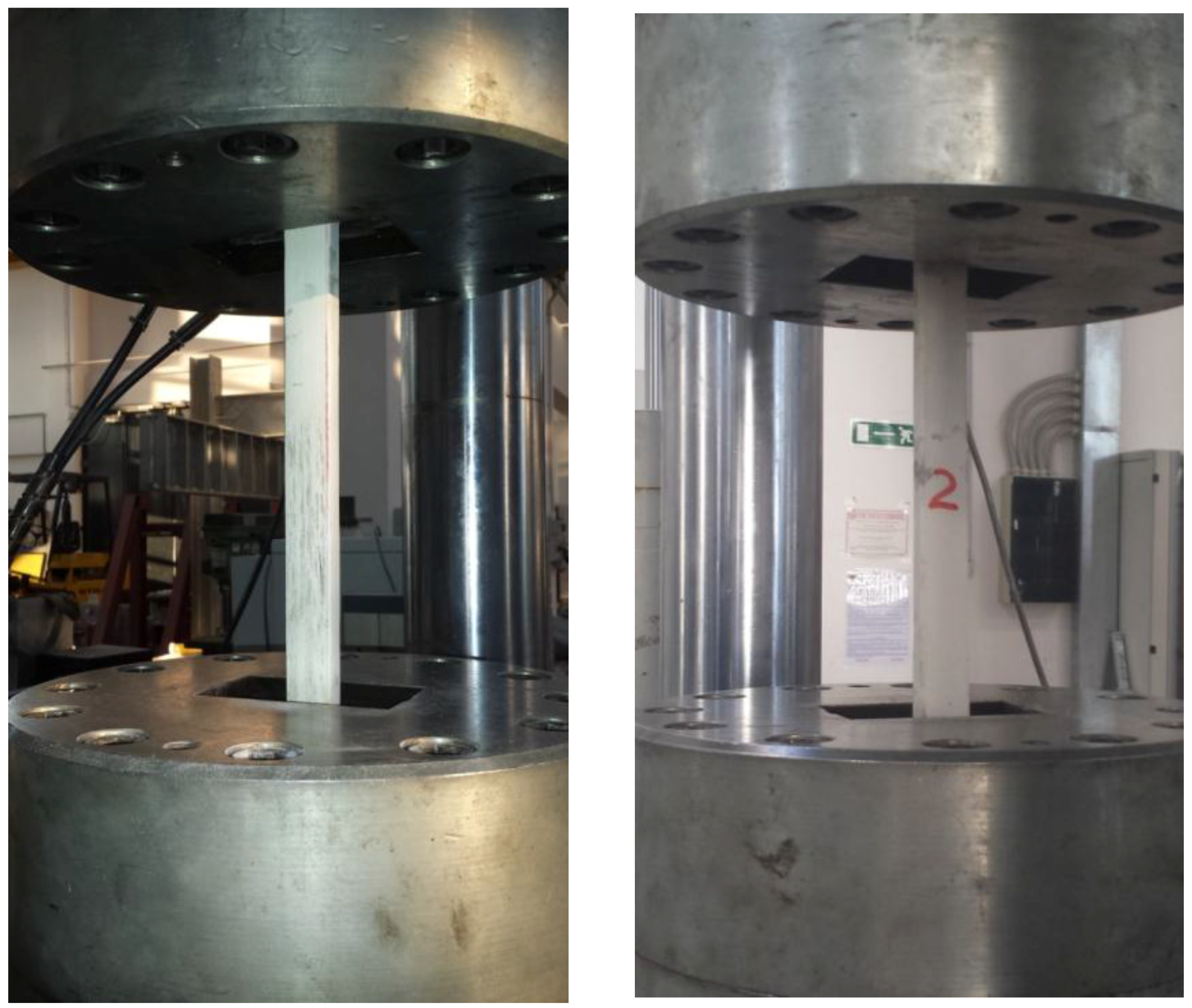
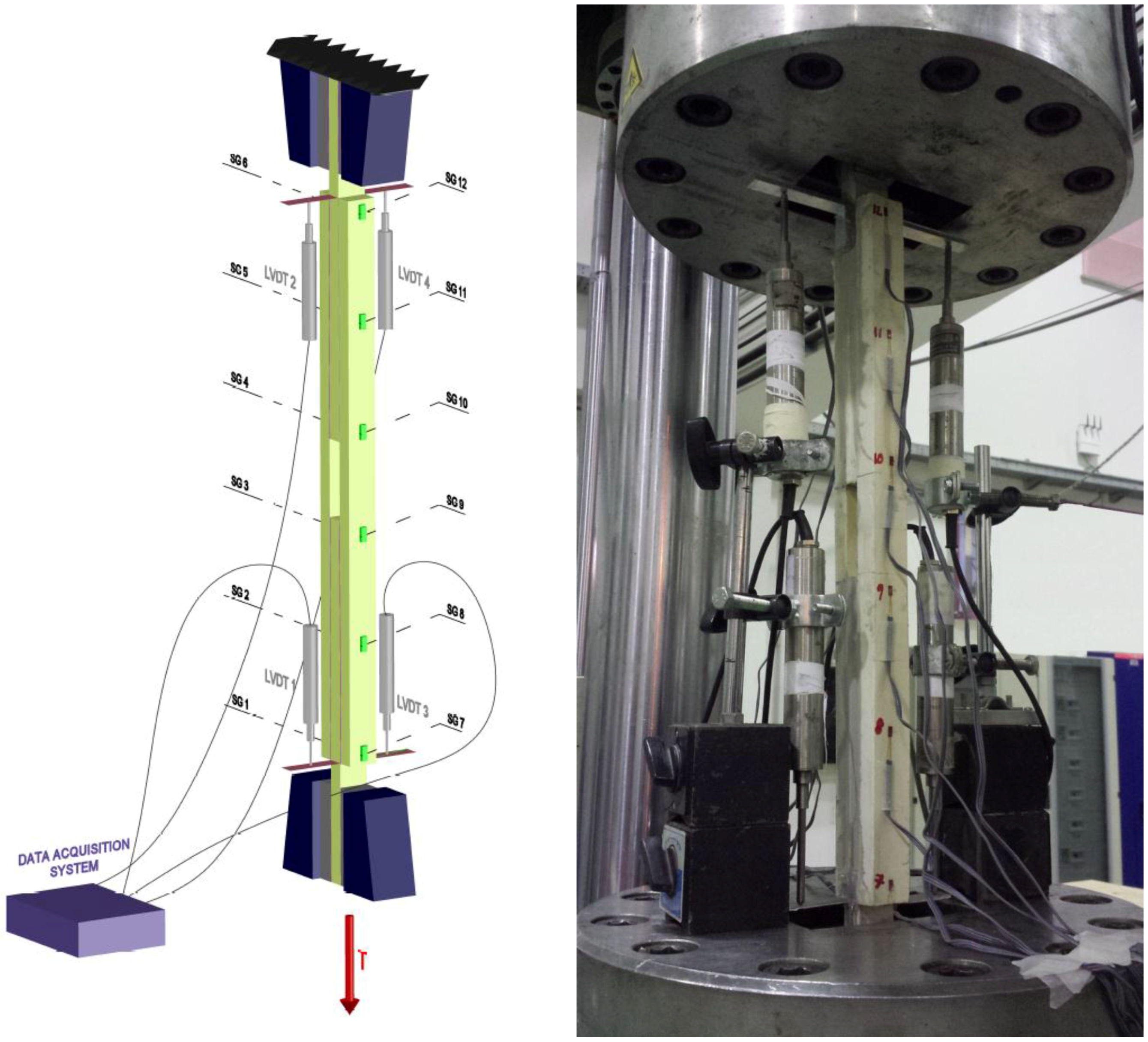
2.1. Experimental Methodology
- Via the preliminary axial tests:
- -
- the elastic properties of the GFRP adherents (to be compared with those given by the manufacturer).
- Via the main tests:
- -
- the elastic stiffness of the joint;
- -
- the elastic limit of the joint;
- -
- the damage stored over any cyclic path;
- -
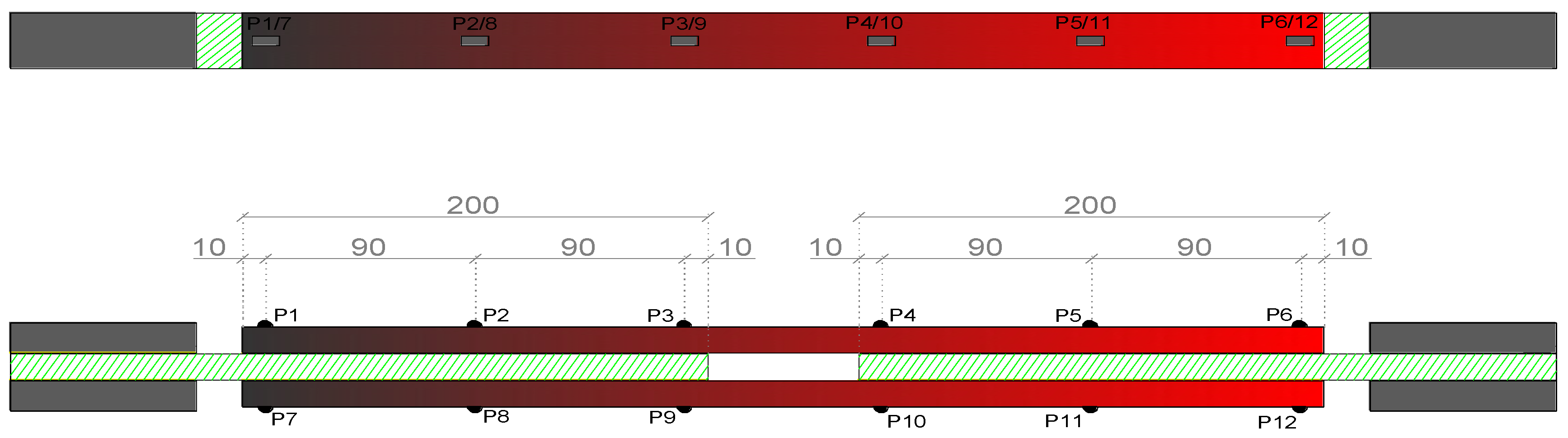
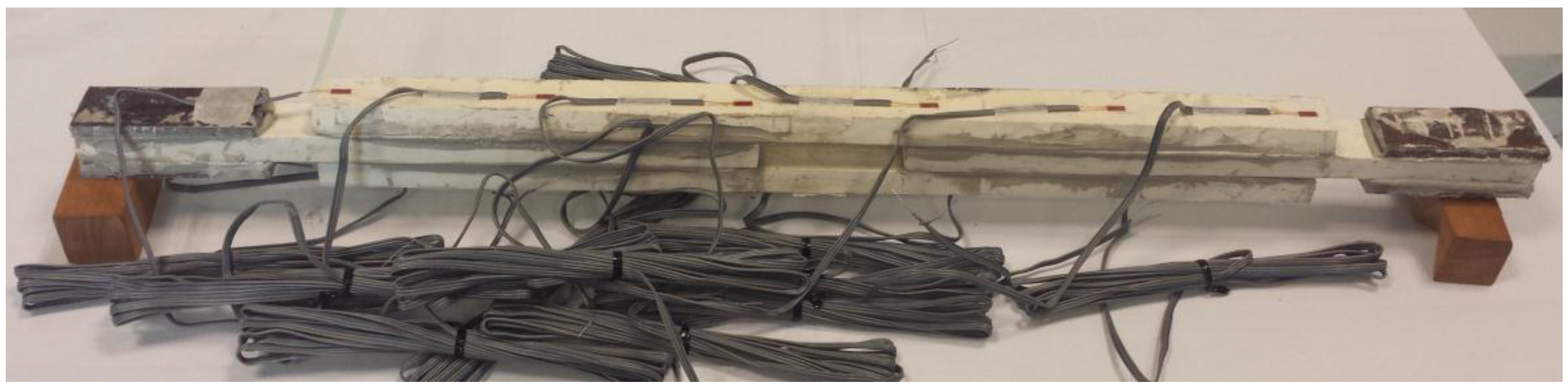
- the evolution of the strains over time within the bonding length; and
- -
- the failure load of the joint.
2.2. A Model of Imperfect Interface with Damage
2.3. Numerical Modelling
3. Results
3.1. Experimental Results
3.1.1. Preliminary Tests
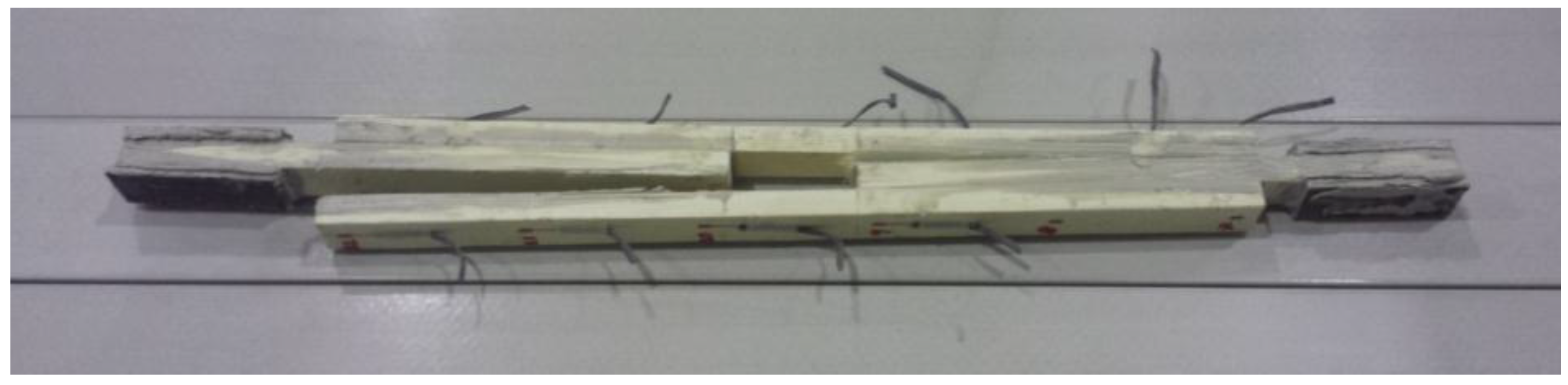
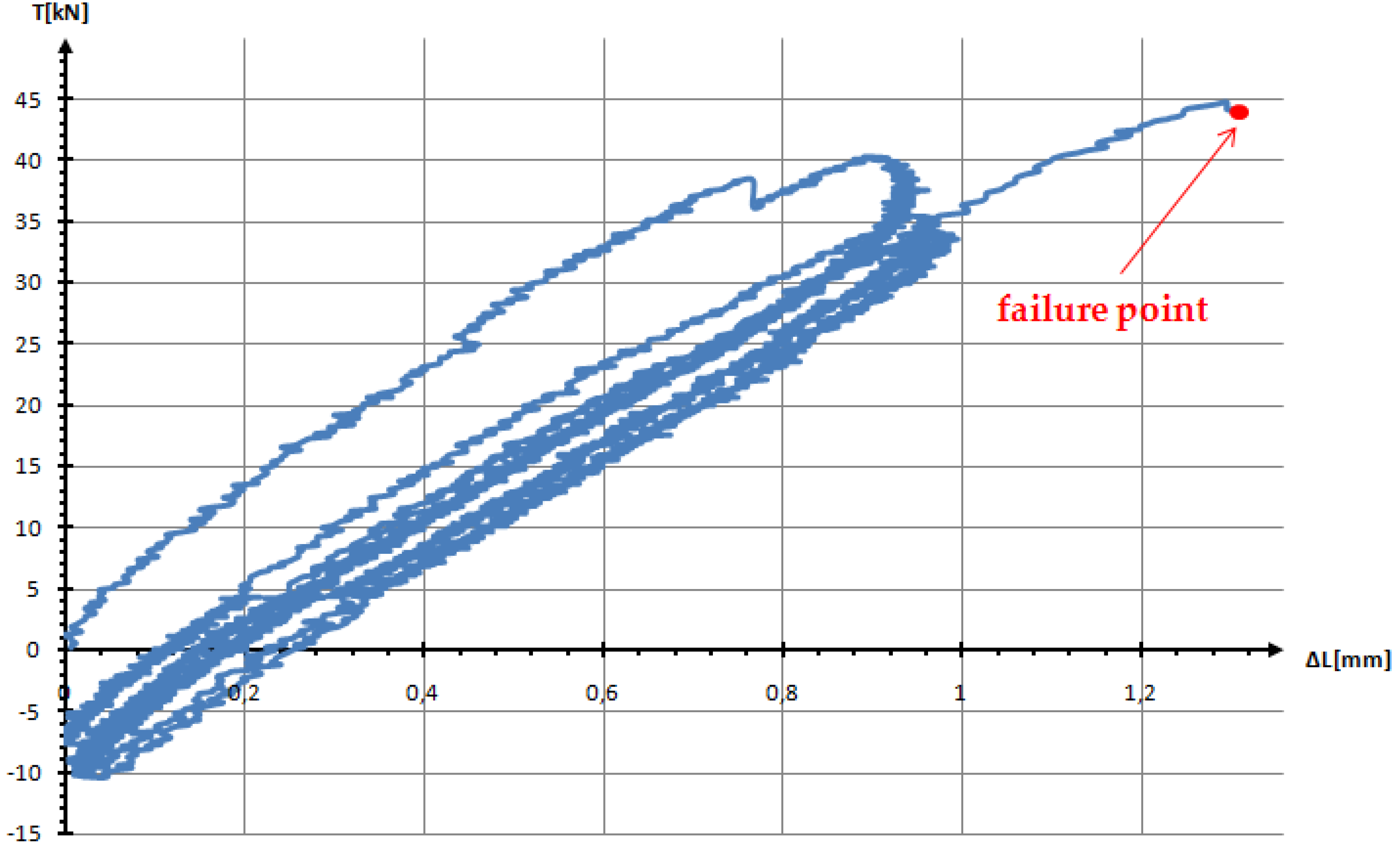
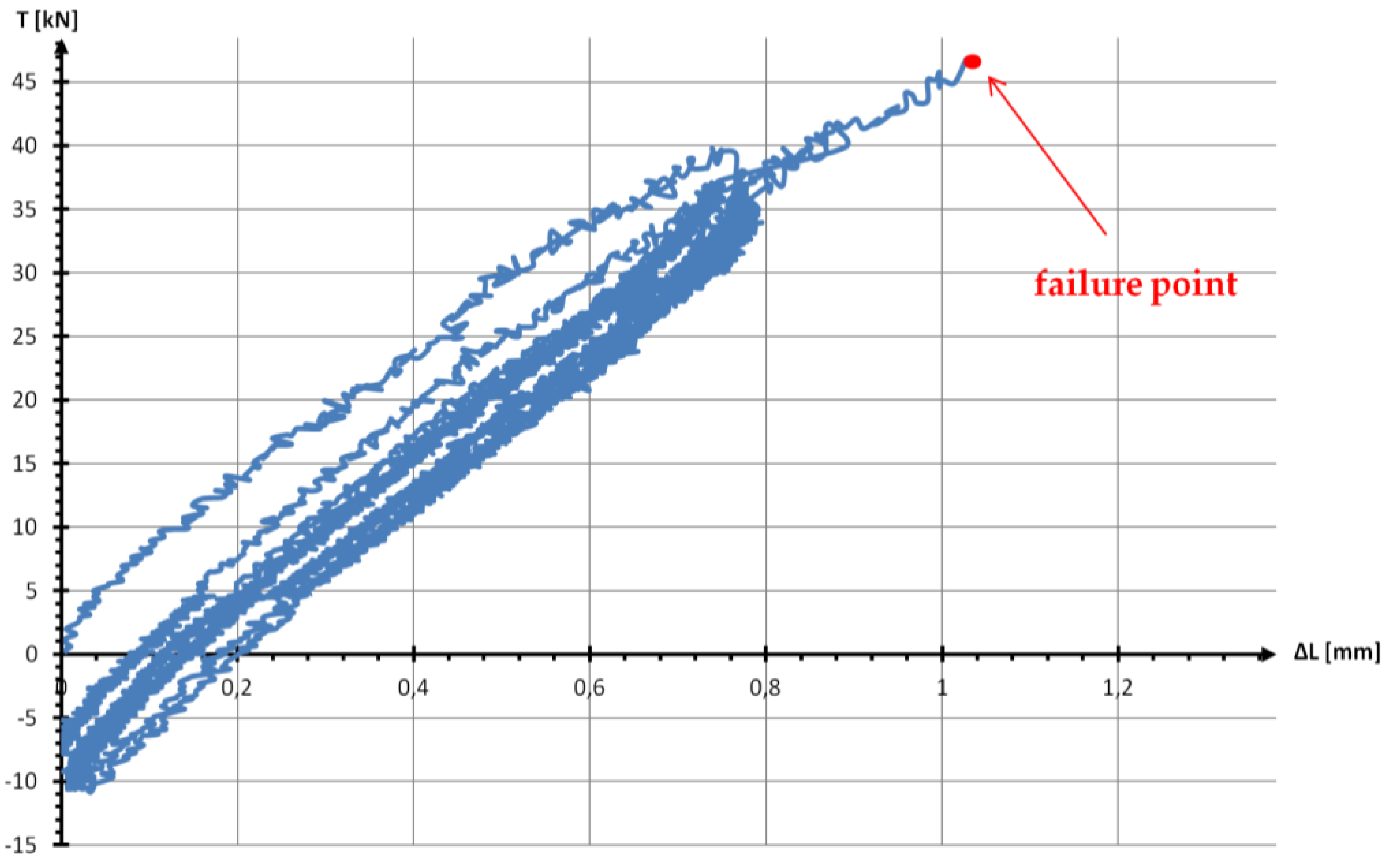
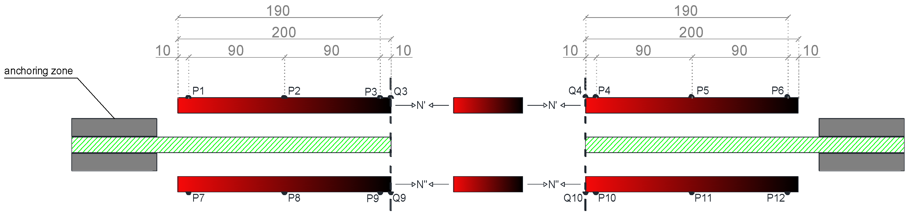
3.1.2. Main Tests
3.2. Numerical Results
- -
- GFRP adherents. The Young’s modulus is equal to E = 37,000 (which is approximatively the stiffness observed in the preliminary tests) and the Poisson’s ratio .
- -
- interfaces. The epoxy resin has a Young’s modulus equal to E = 2000 (according to Table 2), a Poisson’s ratio equal to , the viscosities are equal to , and the length of the representative elementary volume is equal to . For the computation of the crack length, the time increment is set equal to .
4. Discussion
5. Conclusions
Acknowledgments
Author Contributions
Conflicts of Interest
References
- Hasegawa, K.; Crocombe, A.D.; Coppuck, F.; Jewell, D.; Maher, S. Characterising bonded joints with a thick and flexible adhesive layer-Part 1: Fracture testing and behaviour. Int. J. Adhes. Adhes. 2015, 63, 124–131. [Google Scholar] [CrossRef]
- Hasegawa, K.; Crocombe, A.D.; Coppuck, F.; Jewell, D.; Maher, S. Characterising bonded joints with a thick and flexible adhesive layer-Part 2: Fracture testing and behaviour. Int. J. Adhes. Adhes. 2015, 63, 158–165. [Google Scholar] [CrossRef]
- Chaves, F.J.P.; Da Silva, L.F.M.; De Moura, M.F.S.F.; Dillard, D.A.; Esteves, V.H.C. Fracture mechanics tests in adhesively bonded joints: A literature review. J. Adhes. 2014, 90, 955–992. [Google Scholar] [CrossRef]
- Rodríguez, R.Q.; De Paiva, W.P.; Sollero, P.; Rodrigues, M.R.B.; De Albuquerque, É.L. Failure criteria for adhesively bonded joints. Int. J. Adhes. Adhes. 2012, 37, 26–36. [Google Scholar] [CrossRef]
- Narayanamurthy, V.; Chen, J.F.; Cairns, J. Improved model for interfacial stresses accounting for the effect of shear deformation in plated beams. Int. J. Adhes. Adhes. 2016, 64, 33–47. [Google Scholar] [CrossRef]
- Mancusi, G.; Ascione, F. Performance at collapse of adhesive bonding. Compos. Struct. 2013, 96, 256–261. [Google Scholar] [CrossRef]
- Li, J.; Yan, Y.; Zhang, T.; Liang, Z. Experimental study of adhesively bonded CFRP joints subjected to tensile loads. Int. J. Adhes. Adhes. 2015, 57, 95–104. [Google Scholar] [CrossRef]
- Feo, L.; Mancusi, G. Modeling shear deformability of thin-walled composite beams with open cross-section. Mech. Res. Commun. 2010, 37, 320–325. [Google Scholar] [CrossRef]
- Feo, L.; Mancusi, G. The influence of the shear deformations on the local stress state of pultruded composite profiles. Mech. Res. Commun. 2012, 47, 44–49. [Google Scholar] [CrossRef]
- Mancusi, G.; Feo, L. Non-linear pre-buckling behavior of shear deformable thin-walled composite beams with open cross-section. Compos. B Eng. 2013, 47, 379–390. [Google Scholar] [CrossRef]
- Mancusi, G.; Ascione, F.; Lamberti, M. Pre-buckling behavior of composite beams: A mechanical innovative approach. Compos. Struct. 2014, 117, 396–410. [Google Scholar] [CrossRef]
- Costa, I.; Barros, J. Tensile creep of a structural epoxy adhesive: Experimental and analytical characterization. Int. J. Adhes. Adhes. 2015, 59, 115–124. [Google Scholar] [CrossRef] [Green Version]
- Puigvert, F.; Crocombe, A.D.; Gil, L. Fatigue and creep analyses of adhesively bonded anchorages for CFRP tendons. Int. J. Adhes. Adhes. 2014, 54, 143–154. [Google Scholar] [CrossRef]
- Mancusi, G.; Spadea, S.; Berardi, V.P. Experimental analysis on the time-dependent bonding of FRP laminates under sustained loads. Compos. B Eng. 2013, 46, 116–122. [Google Scholar] [CrossRef]
- Marante, M.E.; Flórez-López, J. Three-Dimensional analysis of reinforced concrete frames based on lumped damage mechanics. Int. J. Solids Struct. 2003, 40, 5109–5123. [Google Scholar] [CrossRef]
- Amorim, D.L.D.F.; Sergio, P.B.; Proença, S.P.B.; Flórez-López, J. A model of fracture in reinforced concrete arches based on lumped damage mechanics. Int. J. Solids Struct. 2013, 50, 4070–4079. [Google Scholar] [CrossRef]
- Bonetti, E.; Bonfanti, G.; Lebon, F.; Rizzoni, R. A model of imperfect interface with damage. Meccanica 2016. accepted. [Google Scholar]
- Mauge, C.; Kachanov, M. Effective elastic properties of an anisotropic material with arbitrarily oriented interacting cracks. J. Mech. Phys. Solids 1994, 42, 561–584. [Google Scholar] [CrossRef]
- Tsukrov, I.; Kachanov, M. Effective moduli of an anisotropic material with ellipticalholes of arbitrary orientational distribution. Int. J. Solids Struct. 2000, 37, 5919–5941. [Google Scholar] [CrossRef]
- Klarbring, A. Derivation of the adhesively bonded joints by the asymptotic expansion method. Int. J. Eng. Sci. 1991, 29, 493–512. [Google Scholar] [CrossRef]
- Lebon, F.; OuldKhaoua, A.; Licht, C. Numerical study of soft adhesively bonded joints in finite elasticity. Comput. Mech. 1998, 21, 134–140. [Google Scholar] [CrossRef]
- Rekik, A.; Lebon, F. Identification of the representative crack length evolution in amulti-level interface model for quasi-brittle masonry. Int. J. Solids Struct. 2010, 47, 3011–3021. [Google Scholar] [CrossRef] [Green Version]
- Rekik, A.; Lebon, F. Homogenization methods for interface modeling in damaged masonry. Adv. Eng. Softw. 2012, 46, 35–42. [Google Scholar] [CrossRef]
- Dumont, S.; Lebon, F.; Rizzoni, R. An asymptotic approach to the adhesion of thin stiff films. Mech. Res. Commun. 2014, 58, 24–35. [Google Scholar] [CrossRef]
- Frémond, M. Adhérence des solides. J. Mec. Théor. Appl. 1987, 6, 383–407. (In French) [Google Scholar]
- Fouchal, F.; Lebon, F.; Raffa, M.L.; Vairo, G. An interface model including cracks and roughness applied to masonry. Open Civ. Eng. J. 2014, 8, 263–271. [Google Scholar] [CrossRef]
- Dumont, S.; Lebon, F.; Raffa, M.L.; Rizzoni, R.; Welemane, H. Multiscale modeling of imperfect interfaces and applications. In Computational Methods in Applied Sciences; Springer: Berlin/Heidelberg, Germany, 2016; Volume 41, pp. 81–122. [Google Scholar]
- Raffa, M.L. Micromechanical Modeling of Imperfect Interfaces and Applications. Ph.D. Thesis, University of Rome Tor Vergata, Rome, Italy, 2015. [Google Scholar]
- Nairn, J.A. Numerical implementation of imperfect interfaces. Comput. Mater. Sci. 2007, 40, 525–536. [Google Scholar] [CrossRef]


| - | Value |
|---|---|
| Young’s modulus | |
| Thermal expansion coefficient | |
| Tensile strength | |
| Ultimate tensile strain |
| - | Value | Comments |
|---|---|---|
| Young’s modulus | - | |
| Thermal expansion coefficient | ||
| Bond strength | EN 12188 (angle 50°) | |
| EN 12188 (angle 60°) | ||
| EN 12188 (angle 70°) |
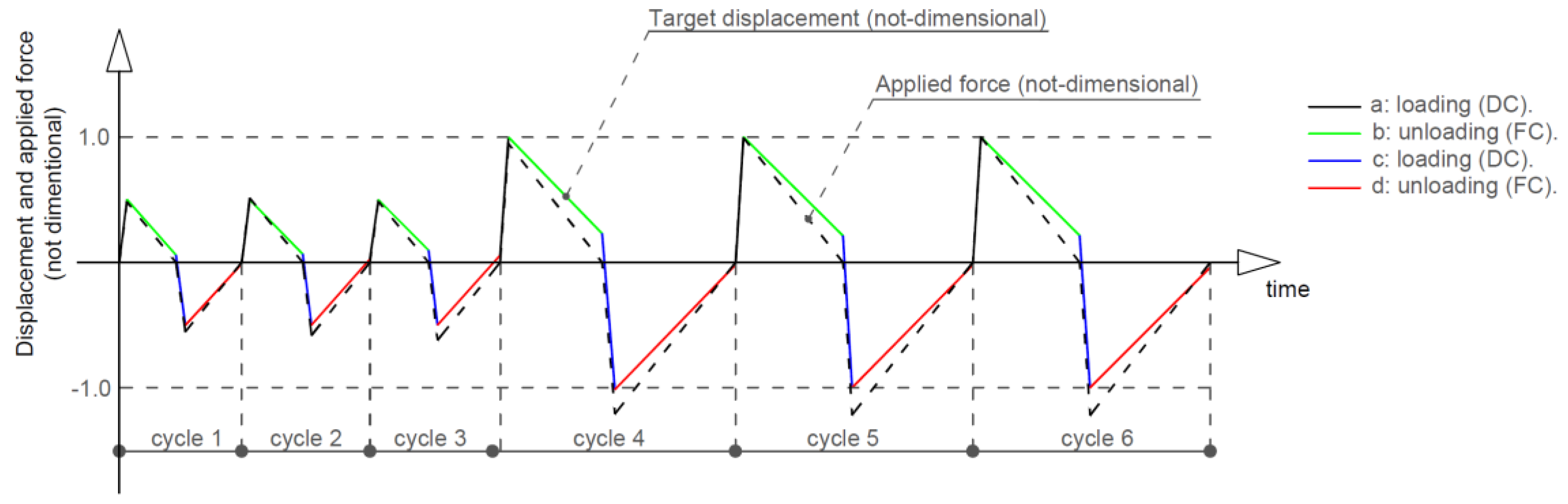
| Cycles | - | (*) | Target | ||
|---|---|---|---|---|---|
| 1, 2, 3 | (a) | loading | DC | +0.50 | mm |
| (b) | unloading | FC | 0.00 | N | |
| (c) | loading | DC | −0.50 | mm | |
| (d) | unloading | FC | 0.00 | N | |
| 4, 5, 6 | (a) | loading | DC | +1.00 | mm |
| (b) | unloading | FC | 0.00 | N | |
| (c) | loading | DC | −1.00 | mm | |
| (d) | unloading | FC | 0.00 | N | |
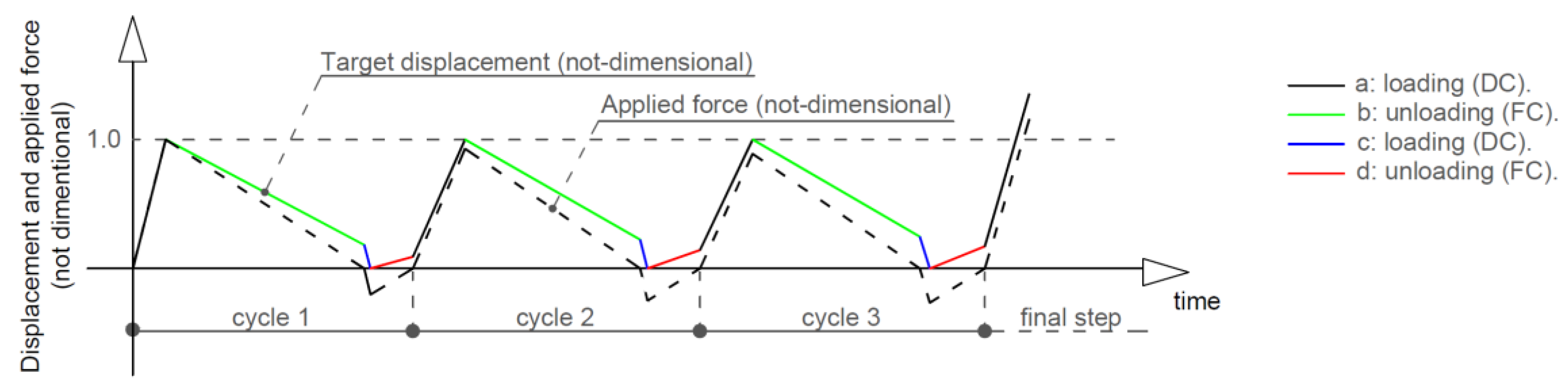
| Cycles | (*) | Target | |||
|---|---|---|---|---|---|
| 1, 2, 3 | (a) | loading | DC | +1.00 | mm |
| (b) | unloading | FC | 0.00 | N | |
| (c) | loading | DC | 0.00 | mm | |
| (d) | unloading | FC | 0.00 | N | |
| Final | loading (**) | DC | + | mm | |
| Cycle | Target | o [%] | 1 [%] | o [MPa] | 1 [MPa] | E01 [MPa] | |||
|---|---|---|---|---|---|---|---|---|---|
| 1 | loading | 1.a | DC | +0.5 mm | 0.000 | 0.161 | 0.00 | 53.14 | 33,642 |
| unloading | 1.b | FC | 0.0 N | 0.161 | 0.006 | 53.14 | 0.00 | 33,349 | |
| loading | 1.c | DC | −0.5 mm | 0.006 | −0.161 | 0.00 | −53.49 | 32,763 | |
| unloading | 1.d | FC | 0.0 N | −0.161 | −0.038 | −53.49 | 0.00 | 41,828 | |
| 2 | loading | 2.a | DC | +0.5 mm | −0.038 | 0.161 | 0.00 | 65.62 | 33,221 |
| unloading | 2.b | FC | 0.0 N | 0.161 | −0.030 | 65.62 | 0.00 | 33,173 | |
| loading | 2.c | DC | −0.5 mm | −0.030 | −0.161 | 0.00 | −42.74 | 32,821 | |
| unloading | 2.d | FC | 0.0 N | −0.161 | −0.064 | −42.74 | 0.00 | 41,227 | |
| 3 | loading | 3.a | DC | +0.5 mm | −0.064 | 0.162 | 0.00 | 72.79 | 32,515 |
| unloading | 3.b | FC | 0.0 N | 0.162 | −0.055 | 72.79 | 0.00 | 32,602 | |
| loading | 3.c | DC | −0.5 mm | −0.055 | −0.161 | 0.00 | −34.32 | 32,542 | |
| unloading | 3.d | FC | 0.0 N | −0.161 | −0.082 | −34.32 | 0.00 | 41,784 | |
| 4 | loading | 4.a | DC | +1.0 mm | −0.082 | 0.321 | 0.00 | 119.45 | 30,426 |
| unloading | 4.b | FC | 0.0 N | 0.321 | −0.006 | 119.45 | 0.00 | 32,971 | |
| loading | 4.c | DC | −1.0 mm | −0.006 | −0.323 | 0.00 | −86.32 | 27,121 | |
| unloading | 4.d | FC | 0.0 N | −0.323 | −0.119 | −86.32 | 0.00 | 38,172 | |
| 5 | loading | 5.a | DC | +1.0 mm | −0.119 | 0.322 | 0.00 | 115.97 | 26,826 |
| unloading | 5.b | FC | 0.0 N | 0.322 | −0.005 | 115.97 | 0.00 | 32,140 | |
| loading | 5.c | DC | −1.0 mm | −0.005 | −0.323 | 0.00 | −83.12 | 26,262 | |
| unloading | 5.d | FC | 0.0 N | −0.323 | −0.107 | −83.12 | 0.00 | 35,486 | |
| 6 | loading | 6.a | DC | +1.0 mm | −0.107 | 0.323 | 0.00 | 109.51 | 26,016 |
| unloading | 6.b | FC | 0.0 N | 0.323 | 0.007 | 109.51 | 0.00 | 31,701 | |
| loading | 6.c | DC | −1.0 mm | 0.007 | −0.323 | 0.00 | −82.81 | 25,243 | |
| unloading | 6.d | FC | 0.0 N | −0.323 | −0.098 | −82.81 | 0.00 | 33,678 | |
| Cycle | Target | o [%] | 1 [%] | o [MPa] | 1 [MPa] | E01 [MPa] | |||
|---|---|---|---|---|---|---|---|---|---|
| 1 | loading | 1.a | DC | +0.5 mm | 0.000 | 0.162 | 0.00 | 54.44 | 33,986 |
| unloading | 1.b | FC | 0.0 N | 0.162 | 0.019 | 54.44 | 0.00 | 36,640 | |
| loading | 1.c | DC | −0.5 mm | 0.019 | −0.162 | 0.00 | −62.66 | 34,932 | |
| unloading | 1.d | FC | 0.0 N | −0.162 | −0.004 | −62.66 | 0.00 | 38,586 | |
| 2 | loading | 2.a | DC | +0.5 mm | −0.004 | 0.161 | 0.00 | 57.97 | 35,174 |
| unloading | 2.b | FC | 0.0 N | 0.161 | 0.021 | 57.97 | 0.00 | 40,150 | |
| loading | 2.c | DC | −0.5 mm | 0.021 | −0.162 | 0.00 | −65.81 | 36,181 | |
| unloading | 2.d | FC | 0.0 N | −0.162 | 0.008 | −65.81 | 0.00 | 37,717 | |
| 3 | loading | 3.a | DC | +0.5 mm | 0.008 | 0.161 | 0.00 | 54.91 | 36,079 |
| unloading | 3.b | FC | 0.0 N | 0.161 | 0.031 | 54.91 | 0.00 | 40,531 | |
| loading | 3.c | DC | −0.5 mm | 0.031 | −0.162 | 0.00 | −70.15 | 36,721 | |
| unloading | 3.d | FC | 0.0 N | −0.162 | 0.018 | −70.15 | 0.00 | 38,001 | |
| 4 | loading | 4.a | DC | +1.0 mm | 0.018 | 0.323 | 0.00 | 107.01 | 35,550 |
| unloading | 4.b | FC | 0.0 N | 0.323 | 0.074 | 107.01 | 0.00 | 41,001 | |
| loading | 4.c | DC | −1.0 mm | 0.074 | −0.328 | 0.00 | −136.69 | 34,713 | |
| unloading | 4.d | FC | 0.0 N | −0.328 | −0.006 | −136.69 | 0.00 | 40,143 | |
| 5 | loading | 5.a | DC | +1.0 mm | −0.006 | 0.323 | 0.00 | 112.47 | 34,268 |
| unloading | 5.b | FC | 0.0 N | 0.323 | 0.069 | 112.47 | 0.00 | 40,975 | |
| loading | 5.c | DC | −1.0 mm | 0.069 | −0.323 | 0.00 | −137.65 | 35,248 | |
| unloading | 5.d | FC | 0.0 N | −0.323 | −0.007 | −137.65 | 0.00 | 40,376 | |
| 6 | loading | 6.a | DC | +1.0 mm | −0.007 | 0.323 | 0.00 | 112.98 | 34,334 |
| unloading | 6.b | FC | 0.0 N | 0.323 | 0.069 | 112.98 | 0.00 | 41,424 | |
| loading | 6.c | DC | −1.0 mm | 0.069 | −0.323 | 0.00 | −138.01 | 35,554 | |
| unloading | 6.d | FC | 0.0 N | −0.323 | −0.013 | −138.01 | 0.00 | 40,253 | |
| Cycle | Target | To [kN] | T1 [kN] | ∆Lo [mm] | ∆L1 [mm] | K01[kN/mm] | |||
|---|---|---|---|---|---|---|---|---|---|
| 1 | loading | 1.a | DC | +1.0 mm | 0.000 | 40.152 | 0.0000 | 0.9004 | 52.165 |
| unloading | 1.b | FC | 0.0 N | 40.152 | 0.000 | 0.9004 | 0.1903 | 46.923 | |
| loading | 1.c | DC | 0.0 mm | 0.000 | −7.728 | 0.1903 | 0.0000 | 47.831 | |
| unloading | 1.d | FC | 0.0 N | −7.728 | 0.000 | 0.0000 | 0.1031 | 53.262 | |
| 2 | loading | 2.a | DC | +1.0 mm | 0.000 | 35.466 | 0.1031 | 0.9290 | 44.073 |
| unloading | 2.b | FC | 0.0 N | 35.466 | 0.000 | 0.9290 | 0.2280 | 44.044 | |
| loading | 2.c | DC | 0.0 mm | 0.000 | −9.482 | 0.2280 | 0.0000 | 49.994 | |
| unloading | 2.d | FC | 0.0 N | −9.482 | 0.000 | 0.0000 | 0.1522 | 63.019 | |
| 3 | loading | 3.a | DC | +1.0 mm | 0.000 | 34.002 | 0.1522 | 0.9675 | 42.659 |
| unloading | 3.b | FC | 0.0 N | 34.002 | 0.000 | 0.9675 | 0.2498 | 43.599 | |
| loading | 3.c | DC | 0.0 mm | 0.000 | −10.142 | 0.2498 | 0.0000 | 46.771 | |
| unloading | 3.d | FC | 0.0 N | −10.142 | 0.000 | 0.0000 | 0.1796 | 59.885 | |
| loading | final | DC | → + mm | 0.000 | 44.207 | 0.1796 | 1.3053 | 42.630 | |
| Cycle | Target | To [kN] | T1 [kN] | ∆Lo [mm] | ∆L1 [mm] | K01 [kN/mm] | |||
|---|---|---|---|---|---|---|---|---|---|
| 1 | loading | 1.a | DC | +1.0 mm | 0.000 | 39.861 | 0.0000 | 0.8898 | 46.582 |
| unloading | 1.b | FC | 0.0 N | 39.861 | 0.000 | 0.8898 | 0.1522 | 57.231 | |
| loading | 1.c | DC | 0.0 mm | 0.000 | −7.116 | 0.1522 | 0.0000 | 60.699 | |
| unloading | 1.d | FC | 0.0 N | −7.116 | 0.000 | 0.0000 | 0.0824 | 77.420 | |
| 2 | loading | 2.a | DC | +1.0 mm | 0.000 | 36.821 | 0.0824 | 0.7781 | 55.994 |
| unloading | 2.b | FC | 0.0 N | 36.821 | 0.000 | 0.7781 | 0.1824 | 56.843 | |
| loading | 2.c | DC | 0.0 mm | 0.000 | −9.187 | 0.1824 | 0.0000 | 63.129 | |
| unloading | 2.d | FC | 0.0 N | −9.187 | 0.000 | 0.0000 | 0.1130 | 82.199 | |
| 3 | loading | 3.a | DC | +1.0 mm | 0.000 | 35.005 | 0.1130 | 0.7827 | 54.876 |
| unloading | 3.b | FC | 0.0 N | 35.005 | 0.000 | 0.7827 | 0.1998 | 56.302 | |
| loading | 3.c | DC | 0.0 mm | 0.000 | −10.576 | 0.1998 | 0.0000 | 62.529 | |
| unloading | 3.d | FC | 0.0 N | −10.576 | 0.000 | 0.0000 | 0.1436 | 77.184 | |
| loading | final | DC | → + mm | 0.000 | 46.784 | 0.1436 | 1.0274 | 54.941 | |
| Position | Position | ||||
|---|---|---|---|---|---|
| rad × 106/N−1 | rad × 106/N−1 | ||||
| P1 | 0.0069 | 0.101 | P7 | 0.0012 | 0.017 |
| P2 | 0.0208 | 0.302 | P8 | 0.0120 | 0.174 |
| P3 | 0.0347 | 0.504 | P9 | 0.0228 | 0.330 |
| Q3 | 0.0363 | 0.526 | Q9 | 0.0240 | 0.347 |
| Q4 | 0.0334 | 0.485 | Q10 | 0.0265 | 0.384 |
| P4 | 0.0320 | 0.464 | P10 | 0.0253 | 0.366 |
| P5 | 0.0188 | 0.272 | P11 | 0.0109 | 0.159 |
| P6 | 0.0055 | 0.080 | P12 | 0.0034 | 0.050 |
| Position | Position | ||||
|---|---|---|---|---|---|
| rad × 106/N−1 | rad × 106/N−1 | ||||
| P1 | 0.0075 | 0.116 | P7 | 0.0075 | 0.116 |
| P2 | 0.0211 | 0.327 | P8 | 0.0162 | 0.251 |
| P3 | 0.0347 | 0.538 | P9 | 0.0249 | 0.386 |
| Q3 | 0.0362 | 0.562 | Q9 | 0.0259 | 0.401 |
| Q4 | 0.0348 | 0.539 | Q10 | 0.0265 | 0.411 |
| P4 | 0.0333 | 0.517 | P10 | 0.0253 | 0.392 |
| P5 | 0.0201 | 0.312 | P11 | 0.0109 | 0.170 |
| P6 | 0.0069 | 0.107 | P12 | 0.0034 | 0.053 |
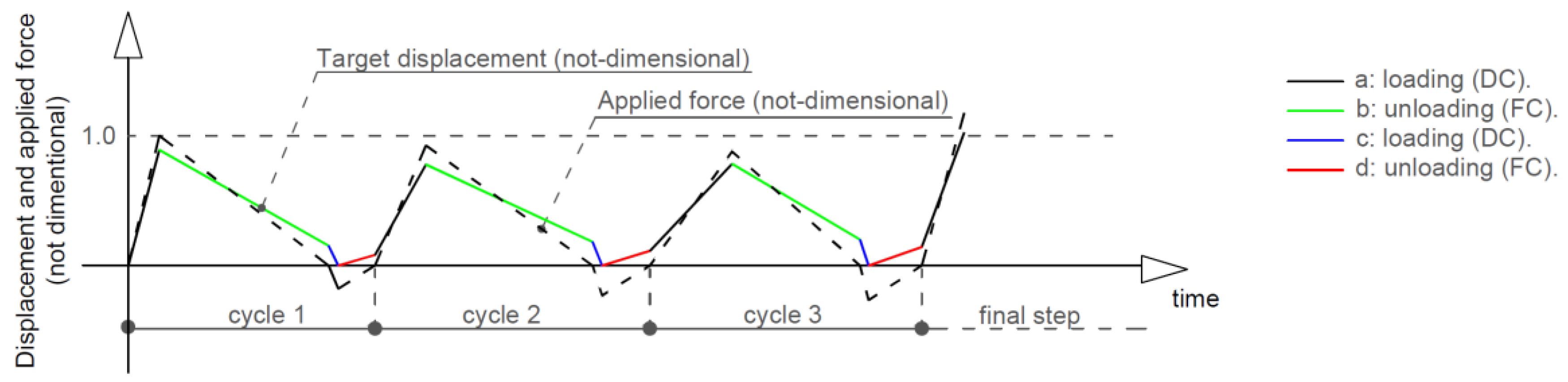
| Cycles | (*) | Target | |||
|---|---|---|---|---|---|
| 2, 3 | (a) | loading | DC | +1.00 | mm |
| (b) | unloading | FC | 0.00 | N | |
| Final | loading | DC | + | mm | |
© 2016 by the authors; licensee MDPI, Basel, Switzerland. This article is an open access article distributed under the terms and conditions of the Creative Commons Attribution (CC-BY) license (http://creativecommons.org/licenses/by/4.0/).
Share and Cite
Orefice, A.; Mancusi, G.; Dumont, S.; Lebon, F. An Experimental/Numerical Study on the Interfacial Damage of Bonded Joints for Fibre-Reinforced Polymer Profiles at Service Conditions. Technologies 2016, 4, 20. https://doi.org/10.3390/technologies4030020
Orefice A, Mancusi G, Dumont S, Lebon F. An Experimental/Numerical Study on the Interfacial Damage of Bonded Joints for Fibre-Reinforced Polymer Profiles at Service Conditions. Technologies. 2016; 4(3):20. https://doi.org/10.3390/technologies4030020
Chicago/Turabian StyleOrefice, Agostina, Geminiano Mancusi, Serge Dumont, and Frédéric Lebon. 2016. "An Experimental/Numerical Study on the Interfacial Damage of Bonded Joints for Fibre-Reinforced Polymer Profiles at Service Conditions" Technologies 4, no. 3: 20. https://doi.org/10.3390/technologies4030020