Designing Closed-Loop Brain-Machine Interfaces Using Model Predictive Control ^†

Abstract

Brain-machine interfaces (BMIs) are broadly defined as systems that establish direct communications between living brain tissue and external devices, such as artificial arms. By sensing and interpreting neuronal activities to actuate an external device, BMI-based neuroprostheses hold great promise in rehabilitating motor disabled subjects, such as amputees. In this paper, we develop a control-theoretic analysis of a BMI-based neuroprosthetic system for voluntary single joint reaching task in the absence of visual feedback. Using synthetic data obtained through the simulation of an experimentally validated psycho-physiological cortical circuit model, both the Wiener filter and the Kalman filter based linear decoders are developed. We analyze the performance of both decoders in the presence and in the absence of natural proprioceptive feedback information. By performing simulations, we show that the performance of both decoders degrades significantly in the absence of the natural proprioception. To recover the performance of these decoders, we propose two problems, namely tracking the desired position trajectory and tracking the firing rate trajectory of neurons which encode the proprioception, in the model predictive control framework to design optimal artificial sensory feedback. Our results indicate that while the position trajectory based design can only recover the position and velocity trajectories, the firing rate trajectory based design can recover the performance of the motor task along with the recovery of firing rates in other cortical regions. Finally, we extend our design by incorporating a network of spiking neurons and designing artificial sensory feedback in the form of a charged balanced biphasic stimulating current.

1. Introduction

Brain-machine interfaces (BMIs) [1,2] are broadly defined as systems that establish direct communications between living brain tissue and external devices such as artificial arm. The major components of these systems include measurements of cortical neuronal activity, extraction of task-relevant motor intention (decoder), and an encoder that feeds back the motor relevant sensory information back to the brain. Thus the brain, the BMI and the prosthetic device together act as a closed-loop BMI. Figure 1 shows a closed-loop BMI design (also known as brain-machine-brain interface (BMBI) [3]).

In the last two decades, BMI based motor intended neural prosthetic systems have been studied extensively [4,5,6,7,8,9,10,11]. In most of these studies, healthy subjects are trained to perform a specific motor task such as reaching or grasping. Recorded data during the performance of the task are then used to develop a mathematical model called decoder. The decoder extracts the kinetic as well as the kinematic motor information from a continuously recorded firing activity of motor relevant cortical neurons. The performance of the decoder is typically measured by applying the decoded information to a prosthetic arm. The online movement based error correction during the reaching task is accomplished by the subject using the available visual feedback information in the absence of the natural proprioception. Therefore these BMIs are considered as partially closed-loop systems in their current formulations where the incorporation of artificial proprioception is neglected in their designs.

In the absence of tactile feedback, these BMIs can fail to differentiate visually similar textures. Similarly, in the absence of proprioception, these BMIs are unable to provide the natural sensation of the arm movement which are both experienced and used by healthy subjects in controlling their natural limb movements. It has been recognized in the BMIs community that the inclusion of sensory feedback from the actuated artificial limb in BMIs is necessary to improve the versatility of motor-based BMIs [12]. It has also recently been shown in [13] that kinesthetic feedback together with the visual feedback can significantly improve the BMI performance.

Recently, attempts have been made towards closing the BMI loop by incorporating artificial texture [3] and proprioception [14,15] information. In these studies, a intra-cortical micro-stimulation (ICMS) technique has been investigated as a promising approach in providing artificial sensation of motor tasks to the brain. The approach relies on a learning paradigm where the subject is trained to differentiate [3] or learn [14,15] artificial sensory feedback in a task-dependent context. Even though the approach is promising for developing future BMIs, the experimental trial and error approach in designing appropriate stimulating sensory input currents may change the natural functionality of the brain. Therefore, a systematic approach that uses optimal feedback control theory is highly desirable towards developing stimulation enhanced next generation BMIs. This approach provides flexibility in designing optimal stimulating sensory input currents and analyzing the closed-loop BMI under various feedback scenarios. It may also reduce the learning effort of the motor task by guiding the movement in the initial learning of the BMI motor task.

The intellectual merit of studying BMIs by taking control-theoretic approach is to exploit all the available degrees of freedom in developing the next generation of BMI-based feedback-enabled neuroprosthetic devices. The development of these feedback-enabled neuroprosthetic devices is necessary for making the prosthetic devices prone to error in decoding and targeting the intended action of the neurons. Moreover, issues such as prosthetic system stability, system reliability, impact of transmission loss, latency and time delays, impact of model complexity and uncertainty, optimality of the modeling and control framework, etc. are critical to the clinical deployment of next generation BMIs.

In recognition of these merits, systematic control-theoretic approaches have recently been taken to optimize the learning process in BMIs [7], rigorously analyze the BMI systems [16,17,18] and design artificial sensory feedback optimally [19,20] by developing a theoretical framework based on optimal feedback control (OFC) theory. For instance, the authors in [7] proposed a learning model to maximize the performance of closed-loop BMIs by leveraging tools such as inverse models and feedback control which are formally embedded in control theory. The authors in [18] developed a theoretical model of BMI experiments using optimal feedback control as a policy for brain control during BMI motor tasks. The framework incorporates visual and proprioceptive feedback in estimating states which are then used to compute optimal control inputs for stimulating neuronal models of the primary motor cortex and the premotor cortex neurons. Using this framework, the authors showed that the experimentally observed abrupt changes in neural modulations when switching to BMI control can be explained using optimal feedback control. In [16], the authors investigated the importance of visual and proprioceptive feedback in BMIs by using a framework of model predictive control in designing optimal stimulus for a single spiking neuron for a single joint movement task based closed-loop BMI. In [17], the authors proposed a stochastic optimal feedback controller as the closed-loop operation of the brain during a BMI performance. Using this framework, they analyzed the performance of open and closed-loop BMIs and explained key phenomenon in closed-loop BMI operation. In particular, they explained the experimentally observed parametric variations in closed-loop operation of BMIs such as the performance deterioration with increasing bin width and diminishing effect of decoder bias in closed-loop BMIs. In [19], the authors showed the first systematic approach in designing optimal artificial sensory feedback in closed-loop BMIs. In particular, the authors proposed an optimal design of feedback-enabled closed-loop BMI and designed artificial proprioceptive feedback using a model predictive controller in a single joint reaching task. The authors further extended their firing rate-based approach [19] to ICMS [20].

In this article, we theoretically demonstrate the recovery of closed-loop performance of a BMI for voluntary single joint extension task by designing an optimal artificial sensory feedback in the absence of the natural proprioceptive feedback pathways. Throughout our analysis, we exclude the treatment of visual feedback as well any form of cortical learning. A theoretical experiment is performed on a firing rate based cortical circuit model of a voluntary control of a single joint extension task to design a BMI. In particular, we design both the Wiener filter and the Kalman filter based decoders and compare their performances. We emphasize the degraded online performance of both decoders in the absence of the proprioceptive feedback. An optimal artificial sensory feedback in the framework of model predictive control is designed to compensate the loss of the natural proprioceptive feedback pathways. We extend our design by including a recurrent network of spiking neurons in the firing rate based neurophysiological cortical circuit model which allow us to design artificial sensory feedback in the form of a charge-balanced biphasic waveform of stimulating input current. We demonstrate the efficacy of our designs by performing simulations.

The remainder of this paper is organized as follows. In Section 2, we describe the neurophysiological cortical circuit model of a voluntary single joint extension task which we used to generate the synthetic data in Section 3. This is followed by the design of both the Wiener filter and the Kalman filter based linear decoders in Section 4. The performance analysis of the designed decoder in the presence and in the absence of the natural proprioception are described in Section 5. We formulate the model predictive control problems and design the artificial sensory feedback in Section 6. The paper ends with discussion.

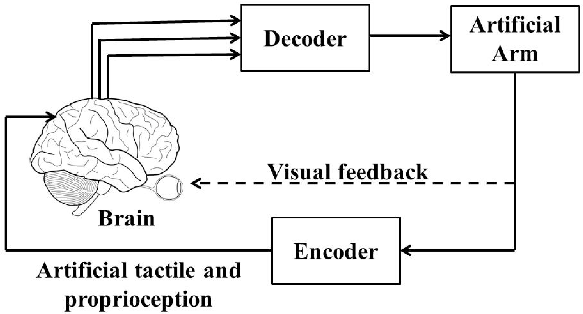
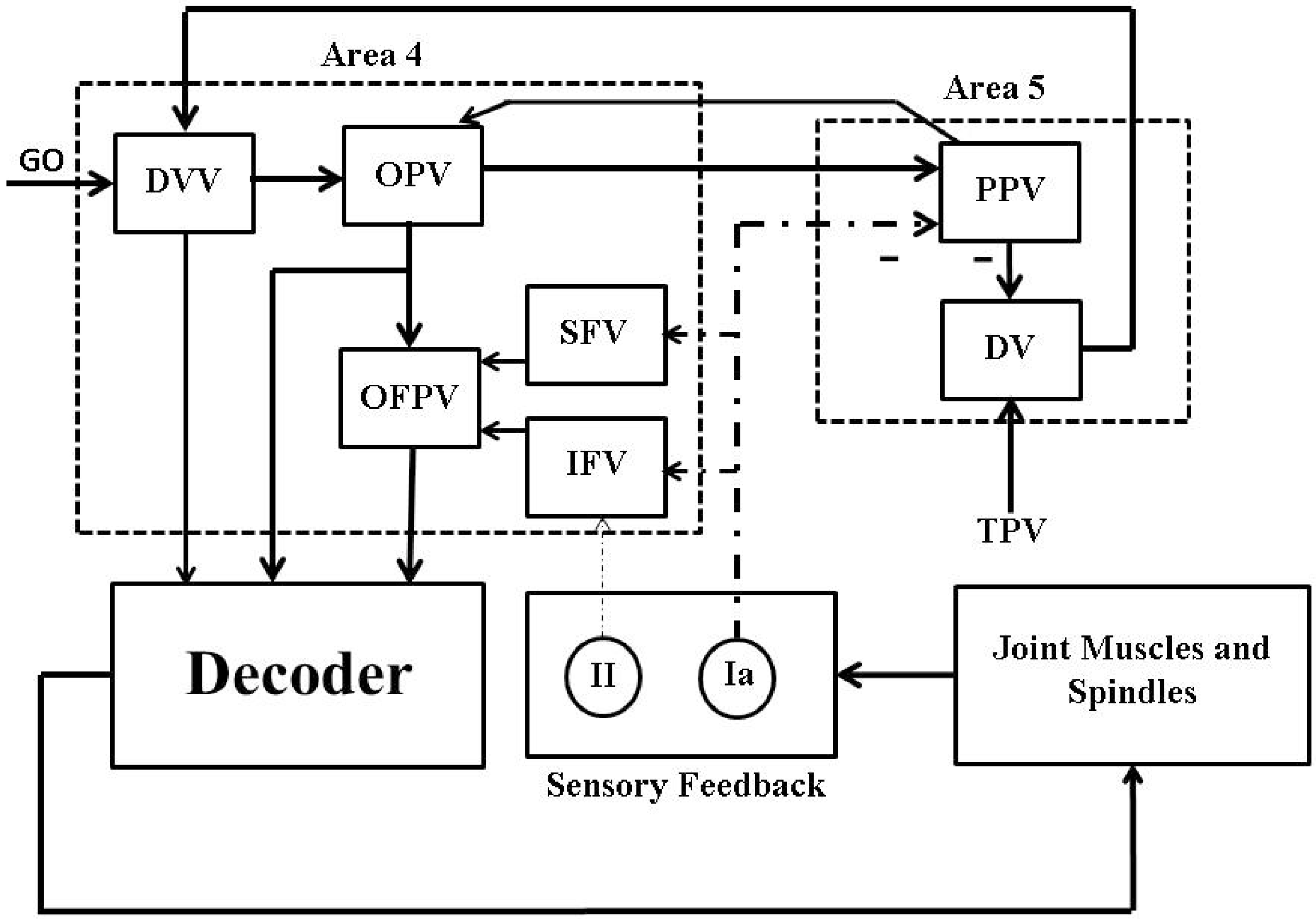
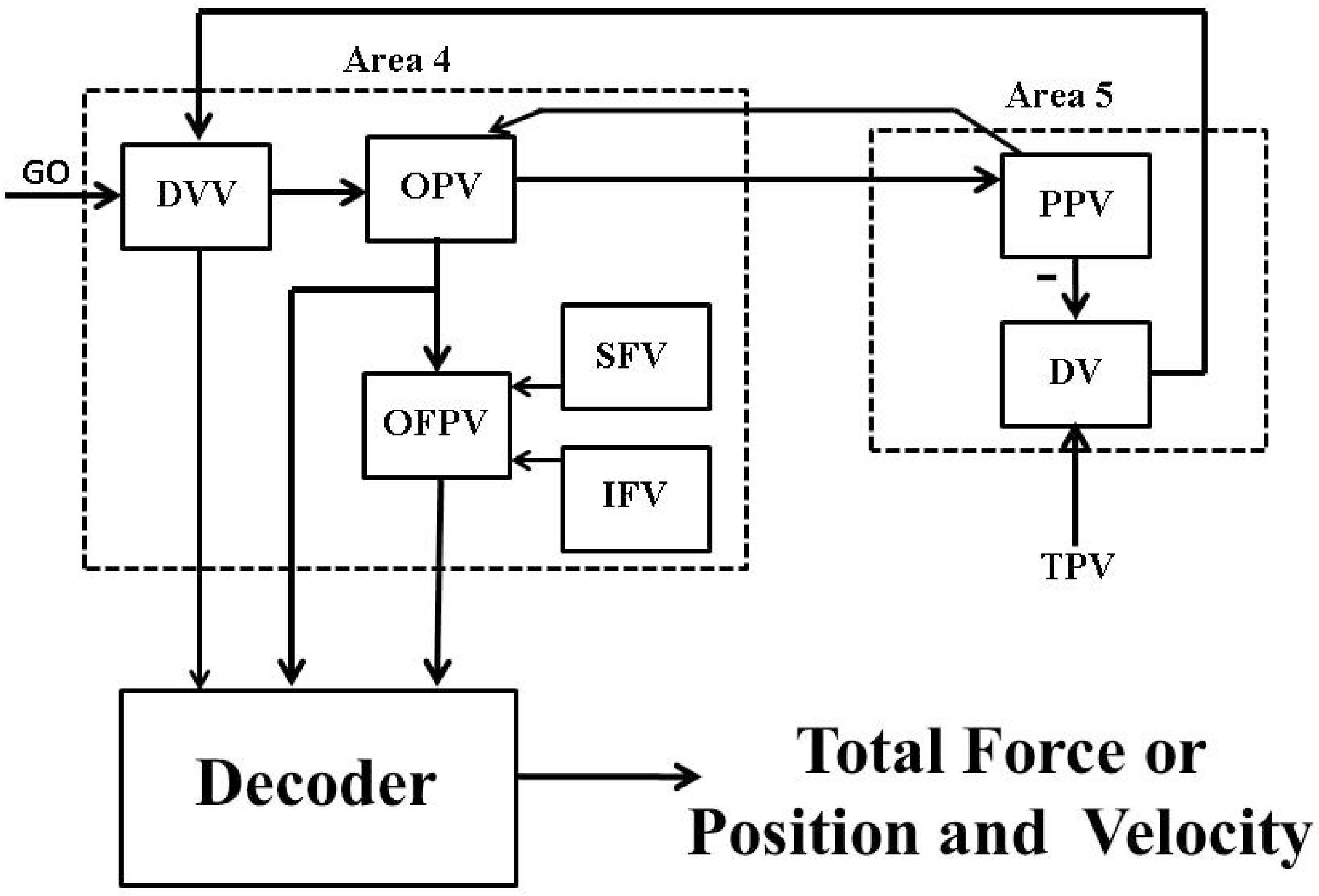
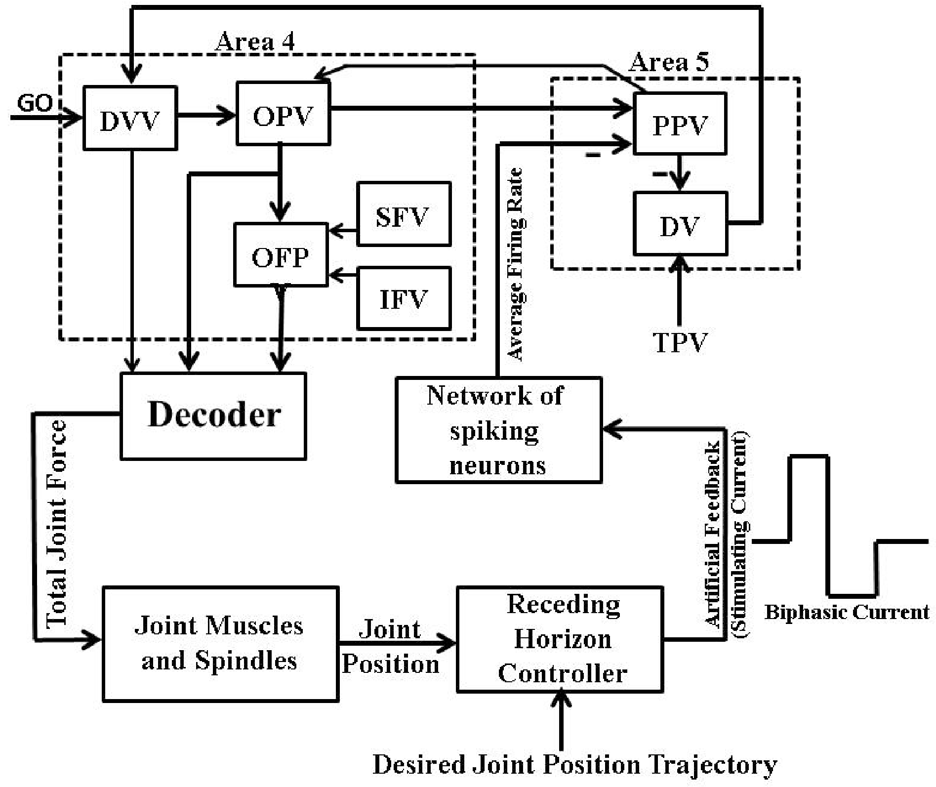
2. Psycho-Physiological Cortical Circuit Model of Single Joint Movement

We used an average firing rate based psycho-physiological cortical circuit model, proposed by [21] and shown in Figure 2, for voluntary control of a single joint movement to design a closed-loop BMI. This minimal model captures the essential cortical pathways as well as the proprioceptive feedback pathways which are relevant during voluntary extension or flexion of a single joint such as elbow. Although the model excludes the treatment of visual feedback during the movement, the model has shown its capability in a qualitative reproduction of several experimentally observed results on voluntary control of a single joint movement. The details of the model and its connection with neurophysiology of a single joint voluntary movement can be found in [21].

Briefly, a population of area 5 (the parietal cortex) “DV” neurons computes the difference between the target and the perceived limb position vectors. The average firing activity of a population of these neurons is represented as

$$r_i\left(t\right)=max\{T_i-x_i\left(t\right)+B^r,0\}.$$

(1)

Here, $0\le r_i\left(t\right)\le 1$ represents the average firing activity of a population of “DV” neurons associated with the agonist muscle i and shows a phasic behavior during the movement. Throughout the paper, we will denote the average firing activity of neurons associated with the agonist muscle i by the subscript i and the corresponding antagonist muscle by the subscript j. $T_i$ is the target position vector (“TPV”) command for the target position of the agonist muscle i. $x_i\left(t\right)$ is the average firing activity of a population of area 5 “PPV” neurons. These neurons continuously compute the present position of the agonist muscle i. $B^r$ is the base firing activity of the “DV” neurons. Continuously computed difference vector information by the area 5 “DV” neurons is then scaled by a population of area 4 (the primary motor cortex (M1)) “DVV” neurons as

$$u_i\left(t\right)=max\{g\left(t\right).(r_i\left(t\right)-r_j\left(t\right))+B^u,0\}.$$

(2)

Here, $u_i\left(t\right)$ is the average firing activity of a population of area 4 “DVV” neurons. $B^u$ is the base firing activity of the “DVV” neurons. $g\left(t\right)$ is an internal “GO” signal which is assumed to be originated from the basal ganglia. “DVV” neurons fire only during the movement and thus their average firing activity shows a phasic-movement time (MT) behavior. The dynamics of the internal “GO” signal is modeled as

$$\frac{\mathrm{d}{\mathrm{g}}^1\left(\mathrm{t}\right)}{\mathrm{d}\mathrm{t}}=ϵ(-g^1\left(t\right)+(C-g^1\left(t\right))g^0),$$

(3a)

$$\frac{\mathrm{d}{\mathrm{g}}^2\left(\mathrm{t}\right)}{\mathrm{d}\mathrm{t}}=ϵ(-g^2\left(t\right)+(C-g^2\left(t\right))g^1\left(t\right)),$$

(3b)

$$g\left(t\right)=g^0\frac{g^2\left(t\right)}{C}.$$

(3c)

Here, ϵ represents a slow integration rate and is treated as constant. C is a constant value at which the “GO” neurons saturate. The area 4 “OPV” neurons receive information from the area 4 “DVV” neurons as well as the area 5 “PPV” neurons and show tonic firing activity. The average firing activity of a population of “OPV” neurons is modeled as

$$\frac{\mathrm{d}{\mathrm{y}}_{\mathrm{i}}\left(\mathrm{t}\right)}{\mathrm{d}\mathrm{t}}=(1-y_i\left(t\right))(\eta x_i\left(t\right)+max\{u_i\left(t\right)-u_j\left(t\right),0\})-y_i\left(t\right)(\eta x_j\left(t\right)+max\{u_j\left(t\right)-u_i\left(t\right),0\}).$$

(4)

Here, η is a scaling factor. The average firing activity of a population of static (${\gamma }_i^S\left(t\right)$) and dynamic (${\gamma }_i^D\left(t\right)$) gamma motoneurons are modeled as

$${\gamma }_i^S\left(t\right)=y_i\left(t\right),$$

(5a)

$${\gamma }_i^D\left(t\right)=\rho max\{u_i\left(t\right)-u_j\left(t\right),0\}.$$

(5b)

Here, ρ is a scaling parameter. The average firing activity of the primary (“Ia”) and the secondary (“II”) muscle spindles afferents are modeled as

$$\begin{array}{cc}\hfill s_i^1\left(t\right)& =S(\theta max\{{\gamma }_i^S\left(t\right)-p_i\left(t\right),0\}\hfill \\ & +\varphi max\{{\gamma }_i^D\left(t\right)-\frac{\mathrm{d}{\mathrm{p}}_{\mathrm{i}}\left(\mathrm{t}\right)}{\mathrm{d}\mathrm{t}},0\}),\hfill \end{array}$$

(6a)

$$s_i^2\left(t\right)=S(\theta max\{{\gamma }_i^S\left(t\right)-p_i\left(t\right),0\}).$$

(6b)

Here, $s_i^1\left(t\right)$ and $s_i^2\left(t\right)$ are the primary and the secondary spindles afferents average firing activity respectively. $p_i$ is the position of the agonist muscle i. θ is the sensitivity of the static nuclear bag and chain fibers. $\varphi$ is the sensitivity of the dynamic nuclear bag fibers. The saturation of spindles afferents activity is given by the function $S\left(\omega \right)=\omega /(1+100{\omega }^2)$. The average firing activity $x_i\left(t\right)$ of a population of area 5 “PPV” neurons is modeled as

$$\begin{array}{cc}\frac{\mathrm{d}{\mathrm{x}}_{\mathrm{i}}\left(\mathrm{t}\right)}{\mathrm{d}\mathrm{t}}=(1-x_i\left(t\right))max\{\mathsf{\Theta }{y}_i\left(t\right)+s_j^1(t-\tau )-s_i^1(t-\tau ),0\}\hfill & \\ & \hfill -x_i\left(t\right)max\{\mathsf{\Theta }{y}_j\left(t\right)+s_i^1(t-\tau )-s_j^1(t-\tau ),0\}.\end{array}$$

(7)

Here, τ is the delay time of the spindles feedback. Θ is a constant gain. The average firing activity $q_i\left(t\right)$ of a population of area 4 “IFV” neurons is modeled as

$$q_i\left(t\right)={\lambda }_{i}max\{s_i^1(t-\tau )-s_i^2(t-\tau )-\mathsf{\Lambda },0\}.$$

(8)

Here, Λ is a constant threshold. The average firing activity $f_i\left(t\right)$ of a population of area 4 “SFV” neurons is modeled as

$$\frac{\mathrm{d}{\mathrm{f}}_{\mathrm{i}}\left(\mathrm{t}\right)}{\mathrm{d}\mathrm{t}}=(1-f_i\left(t\right))h{s}_i^1(t-\tau )-\psi f_i\left(t\right)(f_j\left(t\right)+s_j^1(t-\tau )).$$

(9)

Here, h is a constant gain which controls the strength and speed of an external load compensation. ψ is an inhibitory scaling parameter. The average firing activity $a_i\left(t\right)$ of a population of the area 4 “OFPV” neurons is modeled as

$$a_i\left(t\right)=y_i\left(t\right)+q_i\left(t\right)+f_i\left(t\right).$$

(10)

The average firing activity of these neurons shows a phasic-tonic behavior. The average firing activity ${\alpha }_i\left(t\right)$ of alpha motoneurons is modeled as

$${\alpha }_i\left(t\right)=a_i\left(t\right)+\delta s_i^1\left(t\right),$$

(11)

where δ is a stretch reflex gain. The limb dynamics is described by

$$\begin{array}{cc}\hfill \frac{{\mathrm{d}}^2{\mathrm{p}}_{\mathrm{i}}\left(\mathrm{t}\right)}{\mathrm{d}{\mathrm{t}}^2}& =\frac{1}{I}(M(c_i\left(t\right)-p_i\left(t\right))-M(c_j\left(t\right)-p_j\left(t\right))\hfill \\ & +E_i-V\frac{\mathrm{d}{\mathrm{p}}_{\mathrm{i}}\left(\mathrm{t}\right)}{\mathrm{d}\mathrm{t}}).\hfill \end{array}$$

(12)

Here $p_i\left(t\right)$ is the position of the agonist muscle i within its range of origin-to-insertion distances. $p_j\left(t\right)$ is the position of the antagonist muscle such that $p_i\left(t\right)+p_j\left(t\right)=1$. I is the moment of inertia of the limb. V is the joint viscosity. $E_i$ is the external force applied to the joint. $M(c_i\left(t\right),p_i\left(t\right))=max\{c_i\left(t\right)-p_i\left(t\right),0\}$ represents the total force generated by the agonist muscle i. $c_i\left(t\right)$ is the muscle contraction activity dynamics of which is given by

$$\frac{\mathrm{d}{\mathrm{c}}_{\mathrm{i}}\left(\mathrm{t}\right)}{\mathrm{d}\mathrm{t}}=\nu (-c_i\left(t\right)+{\alpha }_i\left(t\right)).$$

(13)

3. Synthetic Experimental Data Generation for Extension Task

In a typical non-human primate experiment, a monkey is trained to accomplish a given motor task such as reaching or grasping. After the training, spiking activity of single neurons are recorded through implanted multi-channel electrodes from various motor relevant cortical areas such as the primary motor cortex (M1), the premotor area (PMv, PMd), and the primary somatosensory area (S1). Simultaneously, kinetic and kinematic information such as joint torque, velocity and position of the real arm are measured to generate a data set to design a decoder.

In this work, we generated a synthetic experimental data set for voluntary control of a single joint extension task by simulating the system model (1)–(13) in MATLAB (Version R2011b, The MathWorks, Inc., Natick, MA, USA). The target position of the agonist muscle i was set to the desired one at $t=0$. The “GO” signal was turned on at $t=50$ ms. During the initial 50 ms, the system was at the priming state. The initial condition of variables was set to 0 except $x_i\left(0\right)=x_j\left(0\right)=0.5$, $y_i\left(0\right)=y_j\left(0\right)=0.5$, $p_i\left(0\right)=p_j\left(0\right)=0.5$, $u_i\left(0\right)=u_j\left(0\right)=B^u$ and $r_i\left(0\right)=r_j\left(0\right)=B^r$. For the simulation, we used the following model parameters [21]: $I=200$, $V=10$, $\nu =0.15$, $B^r=0.1$, $B^u=0.01$, $\mathsf{\Theta }=0.5$, $\theta =0.5$, $\varphi =1$, $\eta =0.7$, $\rho =0.04$, ${\lambda }_1=150$, ${\lambda }_2=10$, $\mathsf{\Lambda }=0.001$, $\delta =0.1$, $C=25$, $ϵ=0.05$, $\psi =4$, $h=0.01$, $T_1=0.7$ and $\tau =0$.

In BMI experiments, a trial is considered successful if the trained monkey accomplishes the specified motor task in a given time duration. Thus the accomplishment time of the task in successful trials is allowed to vary. In our case, the “GO” signal controls the velocity of the joint movement and thus the accomplishment time of a given task. Therefore we assumed that there is a trial-to-trial variability in the internal “GO” signal. To introduce the trial-to-trial variability in the “GO” signal, we modeled $g^0$ as a Gaussian distributed random variable with mean $0.75$ and variance $0.0025$. For a given trial, $g^0$ is constant. It should be noted that the “GO” signal has no effect on the accuracy of the movement.

We simulated the model and generated synthetic data for 1600 independent trials of the voluntary single joint extension task. In each of these trials, the simulation was performed for the duration of 1.45 s which includes a variable holding period at the target position after the accomplishment of the task. To generate a synthetic data set, we measured the average firing activity of a population of area 4 “DVV”, “OPV”, and “OFPV” agonist and the corresponding antagonist neurons sampled at every 10 ms. Simultaneously, we measured the agonist muscle position $p_i\left(t\right)$, the agonist muscle velocity $v_i\left(t\right)=d{p}_i\left(t\right)/dt$, and the total force difference between the agonist and the corresponding antagonist muscle $\Delta M\left(t\right)=M(c_i\left(t\right),p_i\left(t\right))-M(c_j\left(t\right),p_j\left(t\right))$ at every 10 ms. With this, we created a data set of $233,600$ samples by embedding recorded data from 1600 trials.

4. Wiener and Kalman Filters Based Decoder Designs

Neurophysiological as well as BMI experimental studies have shown the encoding of task-relevant kinetic as well as kinematic motor information in the spike trains of the cortical area 4 neurons. For a given motor task, this motor information is extracted from a continuously recorded spike train of the cortical area 4 neurons by developing a mathematical model called decoder. In the past, several linear and nonlinear decoders have been developed in BMI studies. Among them, the most popular are based on the Wiener filter [22], the Kalman filter and its variations [23,24,25,26,27,28], artificial neural networks [29] and recurrent neural networks [30].

We designed both the adapted Wiener filter [22] and the Kalman filter [28]) based decoder models (linear decoders) to extract the total force difference between the agonist and the corresponding antagonist muscle ($\Delta M\left(k\right)$), the agonist muscle position ($p_i\left(k\right)$), and the agonist muscle velocity ($v_i\left(k\right)$) from the recorded firing activity of the area 4 “DVV”, “OPV”, and “OFPV” neurons and performed comparisons between the performance of these two decoders. Here, $k=1,2,\cdots$ is a discrete sample time at which data were recorded for a given trial. $k=1$ corresponds to $t=0$ ms, $k=2$ corresponds to $t=10$ ms, and so on. We emphasize that these neurons have direct contribution to the spinal cord circuit of the neurophysiological system shown in Figure 2.

4.1. Wiener Filter Based Decoder Design

In a discrete-time adapted Wiener filter based decoder design [22], the relation between $\Delta M\left(k\right)$ and the average firing activity of area 4 neurons, i.e., “DVV”, “OPV”, and “OFPV” neurons can be expressed as

$$\Delta M\left(k\right)={\mathbf{w}}^T\mathbf{z}\left(k\right)+n_1\left(k\right).$$

(14)

Here, $\mathbf{w}$ is a $(L.N)\times 1$ weight vector. L is the number of delay elements. ${(·)}^T$ is the transpose of a vector. $\mathbf{z}\left(k\right)={[z_1\left(k\right),z_1(k-1),\cdots ,z_1(k-L+1),z_2\left(k\right),\cdots ,z_N(k-L+1)]}^T$. $z_m(k-l)$ represents the average firing activity of the population m delayed by l samples. For our system, $z_1=y_i$, $z_2=y_j$, $z_3=u_i$, $z_4=u_j$, $z_5=a_i$, and $z_6=a_j$. Thus, $N=6$. We assumed the number of delay elements $L=10$. Thus the weight vector $\mathbf{w}$ has a dimension of $60\times 1$. We also assumed that there is no measurement noise in obtaining data i.e., $n_1\left(k\right)=0$. Similarly, the relation between ${[p_i\left(k\right),v_i\left(k\right)]}^T$ and the average firing activity of area 4 neurons i.e., “DVV”, “OPV”, and “OFPV” neurons can be expressed as

$${[p_i\left(k\right),v_i\left(k\right)]}^T={\mathbf{W}}^T\mathbf{z}\left(k\right).$$

(15)

Here, ${\mathbf{W}}^T$ is a weight matrix of dimension $60\times 2$. We again assumed that there is no measurement noise in obtaining data.

For consistency with BMI experiments, in this work, we used 220,000 samples of the recorded synthetic data to train the weight vector “$\mathbf{w}$” and the weight matrix “$\mathbf{W}$” of the designed decoders (Equations (14) and (15)). For this, we used the following normalized least mean squares algorithm [22]:

$$\mathbf{w}(k+1)=\mathbf{w}\left(k\right)+\frac{\eta }{\beta +{\left|\right|\mathbf{z}\left(k\right)\left|\right|}^2}\mathbf{z}\left(k\right)e\left(k\right).$$

(16a)

$$\mathbf{W}(k+1)=\mathbf{W}\left(k\right)+\frac{\eta }{\beta +{\left|\right|\mathbf{z}\left(k\right)\left|\right|}^2}\mathbf{z}\left(k\right){\left(\mathbf{e}\left(k\right)\right)}^T.$$

(16b)

Here, η and β are constants. $\left|\right|·\left|\right|$ represents the Euclidean norm. In Equation (16a), $e\left(k\right)$ represents a scalar error between the recorded $\Delta M\left(k\right)$ and the estimated value through Equation (14). In Equation (16b), $\mathbf{e}\left(k\right)$ represents the error vector between the recorded ${[p_i\left(k\right),v_i\left(k\right)]}^T$ and the estimated value through Equation (15). For our study, we set $\eta =0.01$ and $\beta =1$. After the training, we froze the weight vector “$\mathbf{w}$” and the weight matrix “$\mathbf{W}$” to the final adapted value. Then we used the rest of 13,600 samples to validate the performance of both decoders.

Figure 3A,C shows the offline performance of the adapted Wiener filter based decoder in decoding the joint position $p_i\left(k\right)$ and the joint velocity $v_i\left(k\right)$ respectively, as defined by Equation (15), on the test data for 1000 samples. Figure 3E shows the offline performance of the adapted Wiener filter based decoder in decoding the force difference between the agonist and the corresponding antagonist muscle, $\Delta M\left(k\right)$, as defined by Equation (14), on the test data for 1000 samples.

4.2. Kalman Filter Based Decoder Design

The following set of dynamical equations describes the design of the Kalman filter based decoder [28]:

$$\widehat{x}(k\mid k-1)=A\widehat{x}(k-1),$$

(17a)

$$\widehat{P}(k\mid k-1)=A\widehat{P}(k-1)A^T+R,$$

(17b)

$$\widehat{x}\left(k\right)=\widehat{x}(k\mid k-1)+K_k(\mathbf{z}\left(k\right)-C\widehat{x}(k\mid k-1)),$$

(17c)

$$\widehat{P}\left(k\right)=(I-K_{k}C)\widehat{P}(k\mid k-1),$$

(17d)

$$K_k=\widehat{P}(k\mid k-1)C^T{(C\widehat{P}(k\mid k-1)C^T+Q)}^{-1}.$$

(17e)

Here, $\widehat{x}(k\mid k-1)$ and $\widehat{x}\left(k\right)$ represent a priori and a posteriori estimate of the state vector $x\left(k\right)$ of dimension $n\times 1$ at time k respectively. $\widehat{P}(k\mid k-1)$ and $\widehat{P}\left(k\right)$ are the estimate of a priori and a posteriori covariance matrix respectively. $\mathbf{z}\left(k\right)$ is the observation (firing rate) vector of dimension $r\times 1$. $K_k$ is the Kalman gain and I is an identity matrix. $A\in {\mathbb{R}}^{n\times n}$ is the state matrix and is given by $A=X_2{X}_1^T{\left(X_1{X}_1^T\right)}^{-1}$. $C\in {\mathbb{R}}^{r\times n}$ represents the observation matrix and is given by $C=Z{X}^T{\left(X{X}^T\right)}^{-1}$. $R=\frac{1}{D-1}(X_2-A{X}_1){(X_2-A{X}_1)}^T$ and $Q=\frac{1}{D}(Z-CX){(Z-CX)}^T$ are covariance matrices of Gaussian noise sources with mean zero to the state and the observation vectors respectively. The structure of matrices Z, X, $X_1$, and $X_2$ is given by

$$Z=\left(\begin{array}{ccc}{z}_{1,1}& \cdots & z_{1,D}\\ ⋮& \ddots & ⋮\\ z_{r,1}& \cdots & z_{r,D}\end{array}\right)$$

(18a)

$$X=\left(\begin{array}{ccc}{x}_{1,1}& \cdots & x_{1,D}\\ ⋮& \ddots & ⋮\\ x_{n,1}& \cdots & x_{n,D}\end{array}\right)$$

(18b)

$$X_1=\left(\begin{array}{ccc}{x}_{1,1}& \cdots & x_{1,D-1}\\ ⋮& \ddots & ⋮\\ x_{n,1}& \cdots & x_{n,D-1}\end{array}\right)$$

(18c)

$$X_2=\left(\begin{array}{ccc}{x}_{1,2}& \cdots & x_{1,D}\\ ⋮& \ddots & ⋮\\ x_{n,2}& \cdots & x_{n,D}\end{array}\right)$$

(18d)

Here, $z_{i,j}$ represents the $j^{th}$ firing rate data of the $i^{th}$ neuron. $x_{i,j}$ represents the $j^{th}$ data of the $i^{th}$ state.

For our system, $x\left(k\right)\equiv \Delta M\left(k\right)$ ($n=1$) if the total force difference between the agonist and the corresponding antagonist muscle ($\Delta M\left(k\right)$) is extracted, and $x\left(k\right)\equiv {[p_i\left(k\right),v_i\left(k\right)]}^T$ ($n=2$) if the position and the velocity of the agonist muscle are extracted from the average firing activity of area 4 neurons i.e., “DVV”, “OPV”, and “OFPV” neurons. $r=6$ and $D=$ 220,000. $\mathbf{z}\left(k\right)={[y_i\left(k\right),y_j\left(k\right),u_i\left(k\right),u_j\left(k\right),a_i\left(k\right),a_j\left(k\right)]}^T$.

For consistency with the Wiener filter based decoder design, we used 220,000 samples of the recorded synthetic data to compute A, C, R, and Q for both $x\left(k\right)\equiv \Delta M\left(k\right)$ and $x\left(k\right)\equiv {[p_i\left(k\right),v_i\left(k\right)]}^T$. Then we used the rest of $13,600$ samples to validate the performance of the decoder for both cases.

Figure 3F shows the offline performance of the Kalman filter based decoder on the test data for 1000 samples when $x\left(k\right)\equiv \Delta M\left(k\right)$ and Figure 3B,D shows the offline performance of the Kalman filter based decoder on the test data for 1000 samples when $x\left(k\right)\equiv {[p_i\left(k\right),v_i\left(k\right)]}^T$. Clearly, the Kalman filter based decoder performed better than the Wiener filter based decoder on the test data.

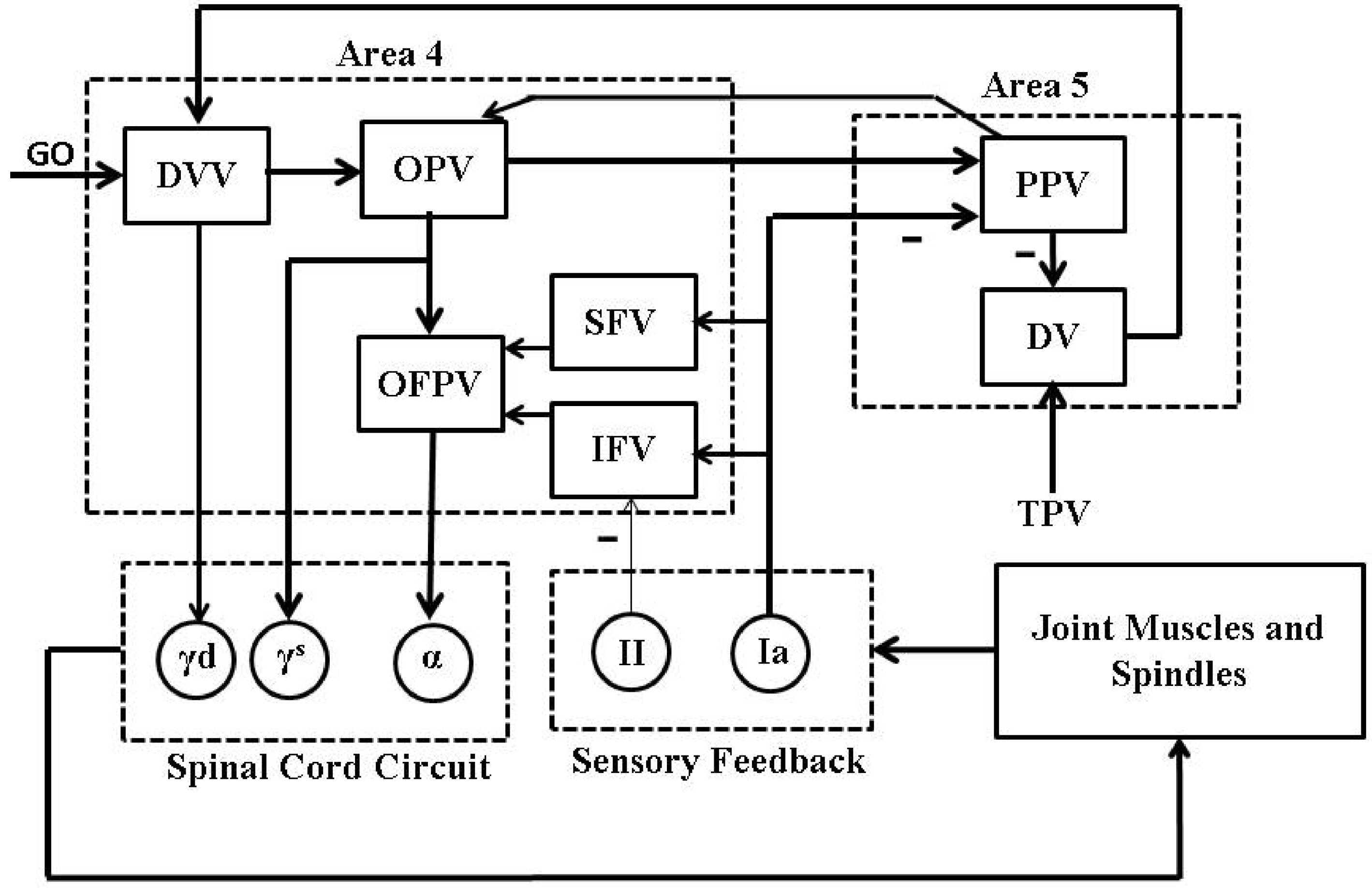
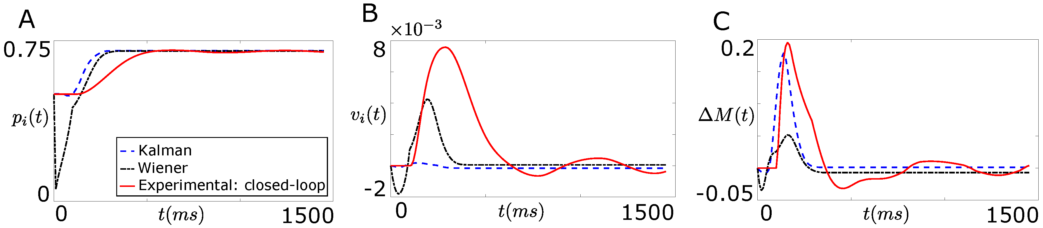
4.3. Comparison of Designed Decoders

We compared the performance of the designed decoders (i.e., the Wiener filter and the Kalman filter) in an open-loop BMI system design shown in Figure 4.

As shown in Figure 4, the average firing activity of area 4 neurons i.e., “DVV”, “OPV”, and “OFPV” neurons are used by the decoder to extract either the total force ($\Delta M\left(k\right)$) or the position ($p_i\left(k\right)$) and the velocity ($v_i\left(k\right)$) of the agonist muscle. To compare the performance of both decoders (i.e., the Wiener filter and the Kalman filter based decoders), We simulated (1)–(10) along with the particular decoder model (i.e., (14)–(16) for the Wiener filter and (17) and (18) for the Kalman filter) and $s_i^1(t-\tau )=s_i^2(t-\tau )=s_j^1(t-\tau )=s_j^2(t-\tau )=0$ and $g^0=0.75$. Remaining model parameters are the same as given in Section 3.

Figure 5A,B compare the open-loop performance of the Wiener filter based decoder and the Kalman filter based decoder with the performance of the closed-loop real system shown in Figure 2 when the extracted information from both decoders is the position ($p_i\left(t\right)$) and the velocity ($v_i\left(t\right)$) of the agonist muscle in real time t respectively. As shown clearly in these figures, the performance of both decoders degrades substantially in the absence of the natural proprioception information. Moreover, the Kalman filter performed better over the Wiener filter in decoding position compared to the velocity of the agonist muscle.

Figure 5C compares the open-loop performance of the Wiener filter based decoder and the Kalman filter based decoder with the performance of the closed-loop real system shown in Figure 2 when the extracted information from both the decoders is the total force ($\Delta M\left(t\right)$) in real time t. As shown in Figure 5C, the performance of both decoders degrades substantially in the absence of the natural proprioception information.

Without the loss of generality, in the rest of the paper, we considered the Wiener filter based decoder design with $\Delta M\left(t\right)$ as the extracted information to design closed-loop BMIs. Note that the described approach can be implemented to other forms of decoders as well.

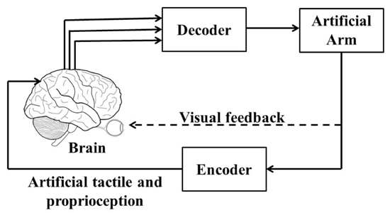
5. Need of a Closed-Loop BMI

We studied the online performance of the Wiener filter based decoder with $\Delta M\left(k\right)$ as the extracted information in the presence and in the absence of the natural proprioceptive feedback information when the decoder interacts with the dynamics of the muscle as shown in Figure 6.

To make a realistic comparison of the performance of the decoder with the neurophysiological (psycho-physiological) system, we first carried out our investigation by studying the performance of the neurophysiological system shown in Figure 2 in the presence and in the absence of the natural proprioceptive feedback i.e., the sensory feedback. For both cases, we simulated (1)–(13) with $g^0=0.75$. The remaining model parameters are the same as given in Section 3 for both cases except $\theta =0$ and $\rho =0$ in the case of no proprioception. This means that the primary (“Ia”) and the secondary (“II”) muscle spindles afferents become inactive (see (6)) in the absence of proprioception.

Figure 7A shows the position trajectory of the agonist muscle i ($p_i\left(t\right)$) in the presence and in the absence of the natural proprioception for the neurophysiological system.

As shown in Figure 7A, the desired position of the agonist muscle i has been achieved in both cases for the neurophysiological system. The result is consistent with a prior neurophysiological experiment where it was shown that a trained monkey (in the absence of visual feedback) can reach the desired target position in the presence and in the absence of proprioception [31].

Next we studied the performance of the closed-loop BMI (decoder) (in the presence of the natural proprioceptive feedback information) and the open-loop BMI (decoder) (in the absence of the natural proprioceptive feedback information) shown in Figure 6. For this, we simulated (1)–(10), (12) and (14). Here we assumed that the limb dynamics is the same for the neurophysiological system and the BMI. For the open-loop BMI, we again set $\theta =0$ and $\rho =0$.

Figure 7B shows the position trajectory of the agonist muscle i ($p_i\left(t\right)$) in the presence and in the absence of the natural proprioception for the closed-loop and the open-loop BMI.

It is clear from Figure 7B that the decoder performance degrades substantially when the decoder, trained with the closed-loop data, is applied on the open-loop system. Since the decoder was trained with the closed-loop firing activity of the area 4 “OPV”, “DVV” and “OFPV” neurons, the firing activity of these neurons must have changed significantly in the absence of the natural proprioception feedback information. To see this, we plotted the firing activity of these neurons in the presence and in the absence of the natural proprioception feedback information for the BMI design shown in Figure 6. Figure 7C shows the firing activity of the area 4 “OPV”, “DVV” and “OFPV” neurons and the area 5 “PPV” neurons in the presence and in the absence of the natural proprioceptive feedback information.

As shown in Figure 7C, the firing activity of cortical neurons deviates significantly from the closed-loop activity in the absence of the natural proprioceptive feedback information. Since the weights of the designed decoder were not adapted to accommodate these significant deviations in the firing activity of the area 4 neurons, the decoder performance degrades substantially in the absence of the natural proprioceptive feedback information. These results clearly show that there is a necessity for designing an artificial proprioceptive feedback to regain the closed-loop performance of the designed decoder in the absence of the natural proprioceptive feedback.

6. Artificial Proprioceptive Feedback Design

As shown in Figure 2, the area 5 “PPV” neurons receive the position feedback information through the primary (Ia) muscle spindles afferents. These neurons then use this proprioceptive feedback information to compute the present position vector command. In the absence of the natural proprioceptive feedback pathways, this feedback information is lost. In order to compensate the lost feedback information of the area 5 “PPV” neurons, we design an artificial sensory feedback in a model predictive control framework. The goal is to recover the closed-loop performance of the decoder (the Wiener filter based decoder with $\Delta M\left(k\right)$ as the extracted information) by providing the designed optimal artificial sensory feedback to the “PPV” neurons in the absence of the natural proprioceptive feedback pathways. Note that we are not designing artificial feedback to compensate the loss of sensory feedback to the area 4 “IFV” and “SFV” neurons in this study. Thus in the absence of the natural sensory feedback, these neurons remain inactive during our analysis.

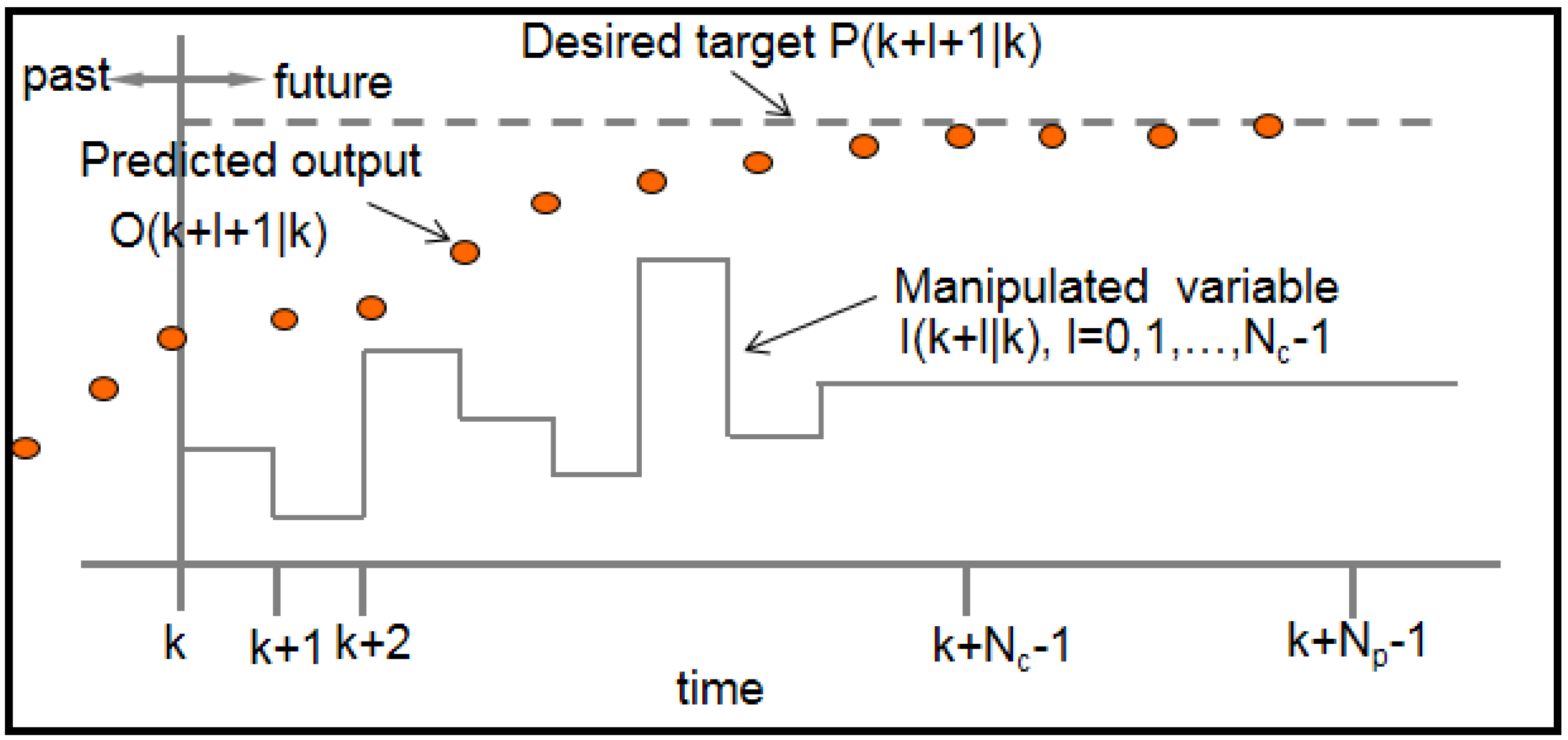
6.1. Model Predictive Control

Model predictive control (MPC) is an optimal control strategy that explicitly incorporates a dynamic model of the system as well as constraints in determining control actions. At each time k, the system measurements are obtained and a model of the system is used to predict future outputs of the system $O_{k+l+1\mid k}$, $l=0,1,2,\cdots ,N_p-1$ as a function of current and future control moves $I_{k+l\mid k}$, $l=0,1,2,\cdots ,N_c-1$. How far ahead in the future the predictions are computed is called the prediction horizon $N_p$ and how far ahead the control moves are computed is called the control horizon $N_c$. Figure 8 illustrates the idea of prediction and control horizon in a model-based receding horizon control strategy.

Using the predictions from the model, the $N_c$ control moves $I_{k+l\mid k}$, $l=0,1,\cdots ,N_c-1$ are optimally computed by minimizing a cost function ${\mathbb{J}}_k$ over the prediction horizon $N_p$ subject to constraints on the control inputs as well as any other constraints on the internal states and outputs of the system as follows:

$$\underset{I_{k+l\mid k},l=0,1,\cdots ,N_c-1}{min}{\mathbb{J}}_k$$

(19)

subjects to constraints on control inputs and the system. A typical quadratic objective cost function may be of the form

$${\mathbb{J}}_k=\sum _{l=0}^{N_p-1}\{{[O_{k+l+1\mid k}-P_{k+l+1\mid k}]}^T{Q}_1[O_{k+l+1\mid k}-P_{k+l+1\mid k}]\}+\sum _{l=0}^{N_c-1}\{I_{k+l\mid k}^T{R}_1{I}_{k+l\mid k}\}.$$

(20)

Here, $P_{k+l+1\mid k}$ is the output to be tracked. The matrices $Q_1$ and $R_1$ are positive semidefinite and positive definite weighting matrices respectively which determine the relative importance of the tracking objective versus control effort. Only the first optimally computed move $I_{k\mid k}$ is implemented out of m computed optimal moves at time k. At the next time $k+1$, new system measurements are obtained and the optimization problem is solved again with the new measurements. Thus, the control and prediction horizon recede by one step as time moves ahead by one step. The measurements at each sampling time provide feedback for rejecting inter-sample disturbances, model uncertainty and noises, all of which cause the model predictions to be different from the true system output.

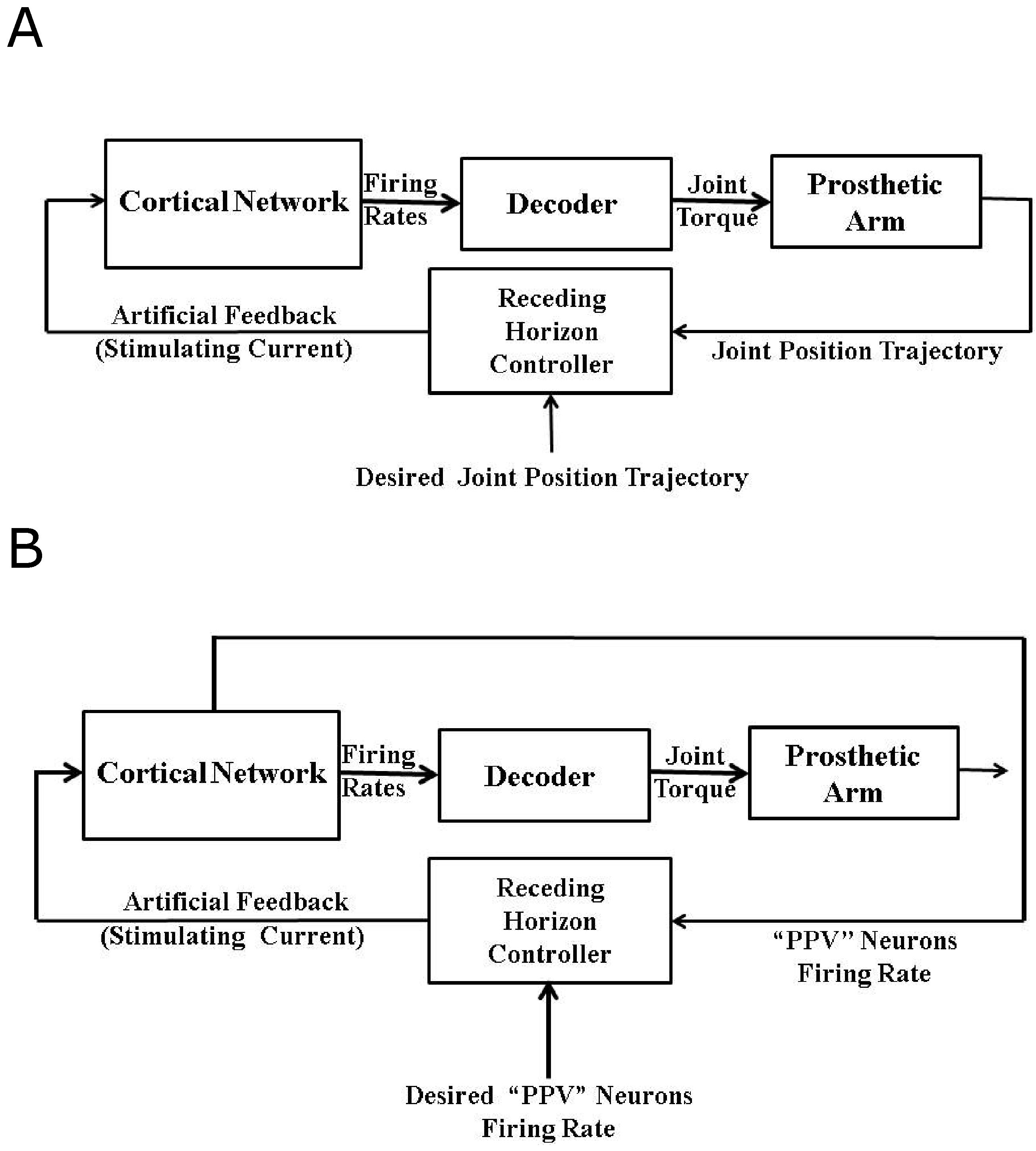
6.2. Firing Rate Based Closed-Loop BMI Design

In order to recover the closed-loop (natural) performance of the decoder, we formulate two control problems in this section. In the first problem, we design an optimal artificial sensory feedback to stimulate the population of area 5 “PPV” neurons such that the position trajectory of the agonist muscle i matches the position trajectory obtained in the presence of the natural proprioception during the reaching task. We call this “Problem 1”. Although we are not treating the visual feedback in this work, this position trajectory tracking problem can be considered equivalent to the BMI experiments where the visual feedback is used by the subject to make online corrections in the trajectory during the reaching task in the absence of proprioception. In the second problem, the goal is to match the average firing activity of the agonist population of “PPV” neurons to its natural firing activity by designing an optimal artificial feedback to stimulate the agonist population of the area 5 “PPV” neurons. We call this “Problem 2”. This firing rate trajectory tracking problem can be considered equivalent to the BMI experiments where the primary somatosensory area (S1) neurons are stimulated artificially to restore the natural proprioception information. Figure 9A,B show the design of a closed-loop BMI operation during the reaching task for problem 1 and problem 2 respectively.

As shown in Figure 9A,B, for both problems we use the MPC strategy (described above) to design the optimal artificial sensory feedback and formulate the following control problem for the systems shown in Figure 9A,B:

$$\underset{I(k\mid k),I(k+1\mid k),\cdots ,I(k+N_c-1\mid k)}{min}{\mathbb{J}}_p\left(k\right)$$

(21a)

such that

$$I(k+l\mid k)\in [-0.5,0.5]for0\le l\le N_c-1,$$

(21b)

$$I(k+l\mid k)=0for{N}_c\le l\le N_p-1.$$

(21c)

Here, $I(k+l\mid k)$ for $l=0,1,\cdots ,N_c-1$ is the designed artificial sensory input. ${\mathbb{J}}_p\left(k\right)={\sum }_{l=0}^{N_p-1}{(O(k+l+1\mid k)-P(k+l+1\mid k))}^2$ is the cost function. Note that $O(k+l+1\mid k)$ and $P(k+l+1\mid k)$ are scalars in our case with $Q_1=R_1=1$ (see Equation (20)). In case of Problem 1 (see Figure 9A), the measured output of the system $O(k\mid k)$ at a given time k is the position of the agonist muscle i, i.e., $p_i(k\mid k)$. $P(·)$ represents the desired position trajectory. In case of Problem 2 (see Figure 9B), the measured output of the system $O(k\mid k)$ at a given time k is the average firing activity of the area 5 “PPV” neurons associated with the agonist muscle i, i.e., $x_i(k\mid k)$. $P(·)$ represents the desired average firing activity of the area 5 “PPV” neurons.

To solve the control problem (21), we first compute the desired position and firing activity trajectory for Problem 1 and 2 respectively. For this, we simulate (1)–(5), (6a), (7), (10), (12) and (14). It should be noted that we have included only the natural sensory feedback (Ia) to the area 5 “PPV” neurons through Equation (6a) for computing the desired trajectory. Thus in the absence of natural proprioception to the area 4 “IFV” and “SFV” neurons, $q_i\left(t\right)=f_i\left(t\right)=0$ in (10). Next we compute $p_i(k+m+1\mid k)$ and $x_i(k+m+1\mid k)$ for $m=0,1,2,\cdots ,N_p-1$ for Problem 1 and 2 respectively. For this, we use a model of the system given by (1)–(4), (10), (12) and (14) along with the following modified firing activity dynamics of the “PPV” neurons:

$$\begin{array}{cc}\hfill \frac{\mathrm{d}{\mathrm{x}}_{\mathrm{i}}\left(\mathrm{t}\right)}{\mathrm{d}\mathrm{t}}& =(1-x_i\left(t\right))max\{\mathsf{\Theta }{y}_i\left(t\right)-I(k+l\mid k),0\}\hfill \\ & -x_i\left(t\right)max\{\mathsf{\Theta }{y}_j\left(t\right)+I(k+l\mid k),0\}.\hfill \end{array}$$

(22)

Here, $I(k+l\mid k)$ is constant during t and $t+10$ ms i.e., between the sample time. Note that the average firing activity of the primary (“Ia”) muscle spindles afferents is set to 0 in (22) (see (7) for the comparison).

With this, we solve the optimization problem (21) numerically in MATLAB for both problems. We use the MATLAB optimization function “fmincon” with the sequential quadratic programming “sqp” algorithm. For both problems, we set $N_c=5$ and $N_p=30$. Figure 10A shows the performance of the controller in tracking the desired position trajectory of the agonist muscle i for “Problem 1”.

As shown in Figure 10A, the controller performs well in tracking the desired position trajectory. Also the stimulation of the area 5 “PPV” neurons by the designed optimal artificial sensory feedback recovers the closed-loop velocity trajectory, as shown in Figure 10B. Thus the designed optimal artificial sensory feedback is sufficient in recovering the closed-loop performance of the decoder in the absence of the natural proprioceptive feedback pathways. Next we wonder if the designed optimal artificial sensory feedback in “Problem 1” also recovers the natural average firing activity of the cortical neurons.

Figure 10C shows the average firing activity of the cortical area 4 and 5 neurons during the reaching task. As shown in this figure, the average firing activity of the cortical area 4 and 5 neurons during the artificial stimulation differs significantly from the natural one. This shows that although the artificial stimulation of the “PPV” neurons through the design of “Problem 1” recovers the closed-loop performance of the decoder, it fails to recover the natural firing activity of the cortical neurons.

Next we study the performance of the designed controller for “Problem 2” (see Figure 9B). Remember that the objective of the controller here is to track the natural average firing activity of the area 5 “PPV” neurons by designing optimal artificial sensory input to the “PPV” neurons. Figure 11A shows the average firing activity of the cortical area 4 and 5 neurons.

As shown in the bottom right plot of Figure 11A, the designed controller performs well in tracking the natural firing activity of the area 5 “PPV” neurons. Moreover, the stimulation results in recovering the natural firing activity of the area 4 cortical neurons.

Figure 11B,C show the position and velocity trajectory of the agonist muscle i during the movement. As shown in these figures, the decoder recovers the closed-loop (natural) performance in this case. This shows that the designed controller in “Problem 2” not only recovers the closed-loop performance of the decoder but also recovers the natural firing activity of the cortical neurons through the optimal artificial stimulation.

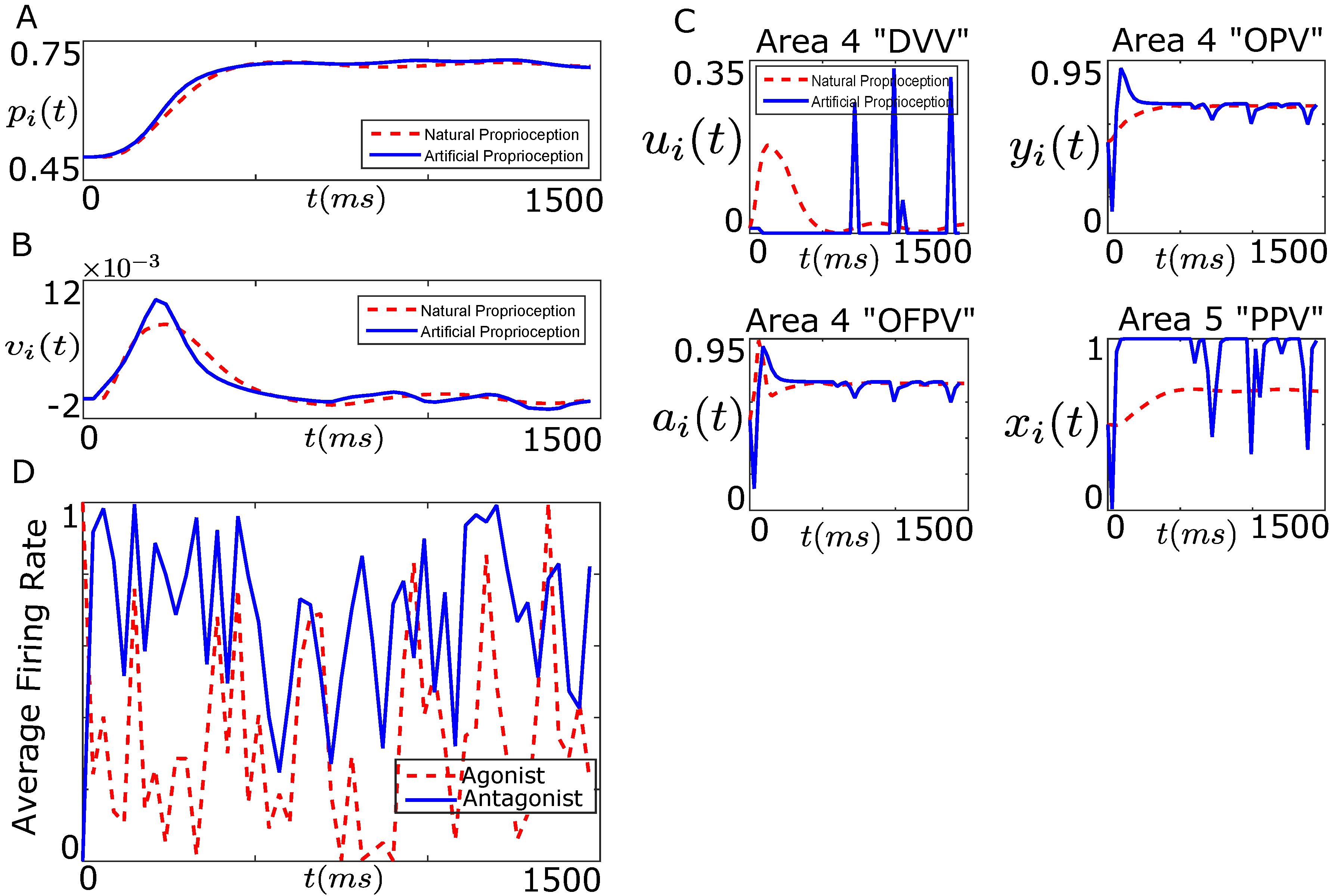
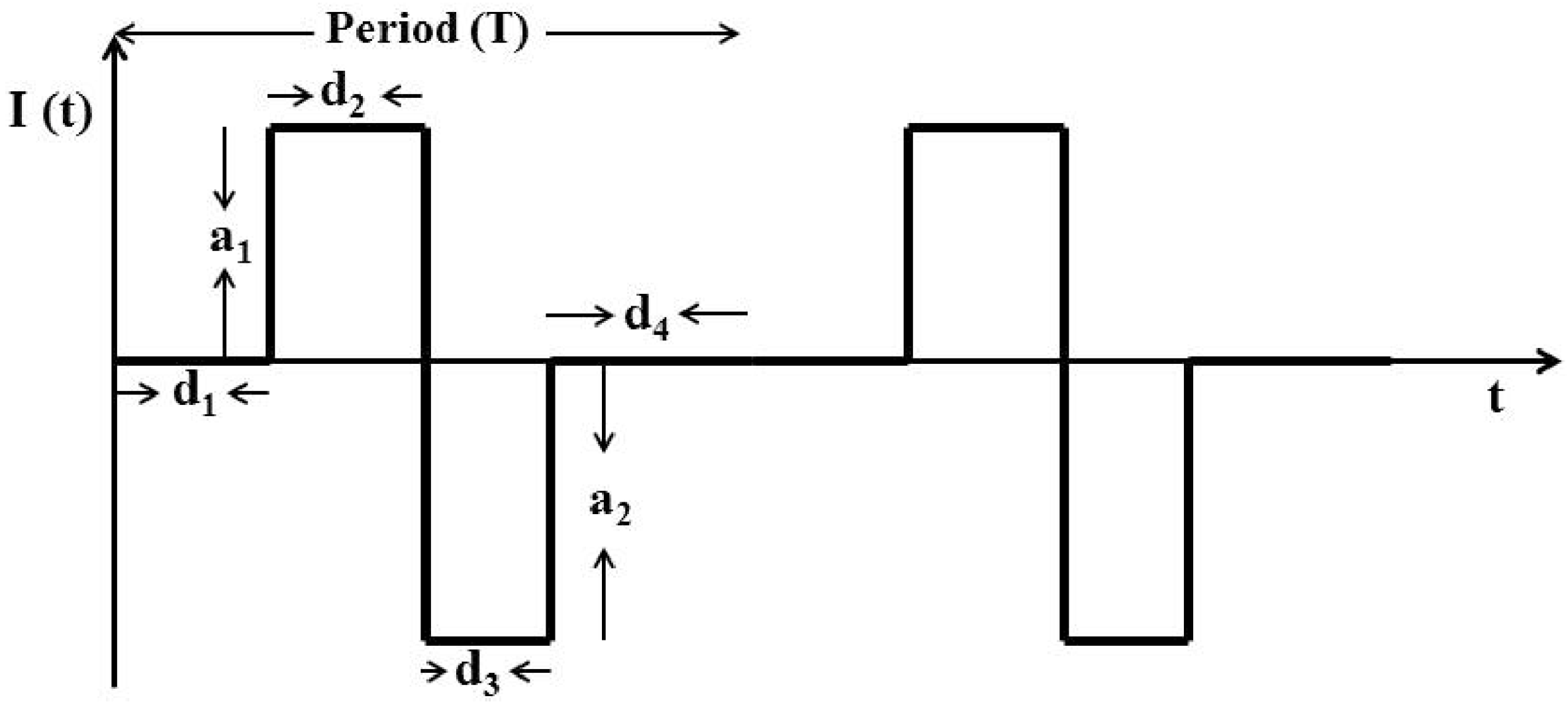
6.3. Intracortical Micro-Stimulation Based Closed-Loop BMI Design

In the previous section, we focused on designing optimal artificial proprioception stimuli in the form of average firing rates. However in experimental BMIs studies, intracortical micro-stimulation (ICMS) based currents in a charge-balanced biphasic waveform are typically used to stimulate cortical sensory neurons and thus to provide artificial sensory feedback during closed-loop operation of BMIs [3,14,32].

Therefore, we modified the MPC-based closed-loop BMI design shown in Figure 9A which allowed us to use such waveform of currents in the present firing activity based framework, as shown in Figure 12.

We modeled the “Network of spiking neurons” in Figure 12 by a recurrent network of the Integrate-and-Fire neurons with dynamics [33]

$${\tau }_k\frac{\mathrm{d}{v}_k\left(t\right)}{\mathrm{d}t}=-v_k\left(t\right)+R_s{I}_k\left(t\right)$$

(23a)

$$I_k\left(t\right)=I_k^s\left(t\right)+I^E\left(t\right)$$

(23b)

$$I_k^s\left(t\right)=-g_k\left(t\right)(v_k\left(t\right)-E)$$

(23c)

$$g_k\left(t\right)=\sum _{l\ne k=1}^{N_k}\sum _f{w}_{l}K(t-t_l^f)$$

(23d)

$$K(t-t_l^f)=\frac{q_l}{{\tau }_l}(t-t_l^f)exp(-\frac{t-t_l^f}{{\tau }_l})\mathsf{\Theta }(t-t_l^f),$$

(23e)

where $v_k\left(t\right)$ is the membrane potential of neuron k at time t, ${\tau }_k$ is the membrane time constant of neuron k and $R_s$ is the membrane resistance. $I_k\left(t\right)$ is the total input current to the neuron k and is the sum of the synaptic current $I_k^s\left(t\right)$ and the stimulating current $I^E\left(t\right)$. $v_k\left(t\right)$ is reset to $v_r$ whenever $v_k\left(t\right)$ exceeds a constant firing threshold $v_{th}$ and an action potential is assumed at this time. $g_k\left(t\right)\ge 0$ is the excitatory conductance and E is the excitatory membrane reversal potential. $N_k$ is the total number of presynaptic neurons to the neuron k, $w_l$ is the weight of the synapse from the $l^{th}$ neuron to the post-synaptic neuron k, $t_l^f$ is the time of the $f^{th}$ incoming action potential from the $l^{th}$ presynaptic neuron, $K(t-t_l^f)$ is the stereotypical time course of postsynaptic conductance following presynaptic spikes, $q_l$ is the maximum conductance transmitted by the $l^{th}$ neuron, and $\mathsf{\Theta }(t-t_l^f)$ is the heavy-side function.

We considered a fully recurrent network of 3 excitatory neurons to represent both the agonist population and the antagonist population of neurons. Network parameters for both populations are provided in Appendix A.1. We computed the average firing rate from the spiking activity of both agonist and antagonist populations as the ratio of the number of spikes in a time window of $T_s=30$ ms and the total number of neurons in individual population, i.e., 3.

We used a rectangular charge-balanced biphasic waveform shown in Figure 13 to design the stimulating current. Here $a_1$, $a_2$, $d_1$, $d_2$, $d_3$ and $d_4$ characterize a single biphasic pulse of the current $I^E\left(t\right)$. The symmetric form of this current minimizes tissue damage, prevents irreversible electrode corrosion and avoids release of toxic metal oxides [34]. This form of current is also the accepted practice in various microstimulation applications such as vestibular prosthesis [35], cochlear implant [36], FES [37,38], DBS [39], retinal prosthesis [40], and BMIs [3,14].

We formulated the following optimal control problem in the MPC framework to recover the closed-loop (natural) performance of the decoder:

$$\underset{\mathit{\beta }\left(k\right|k),\mathit{\beta }(k+1|k),\cdots ,\mathit{\beta }(k+N_c-1|k)}{min}{\mathbb{J}}_p\left(k\right),$$

(24a)

such that

$$a_1(k+l\mid k)\in [0,A_{max}]for0\le l\le N_c-1,$$

(24b)

$$a_2(k+l\mid k)\in [A_{min},0]for0\le l\le N_c-1,$$

(24c)

$$d_i(k+l\mid k)\ge 0fori=1,2,3,0\le l\le N_c-1,$$

(24d)

$$n_t(k+l\mid k)\in \{1,2,3,\cdots \}for0\le l\le N_c-1,$$

(24e)

$$n_t(k+l\mid k)\sum _{i=1}^4{d}_i(k+l\mid k)=T_{s}for0\le l\le N_c-1,$$

(24f)

$$d_2(k+l\mid k)a_1(k+l\mid k)=d_3(k+l\mid k)a_2(k+l\mid k)for0\le l\le N_c-1.$$

(24g)

Here, $\mathit{\beta }(k+l|k)={[a_1(k+l\mid k),a_2(k+l\mid k),d_1(k+l\mid k),d_2(k+l\mid k),d_3(k+l\mid k),n_t(k+l\mid k)]}^{{}^{\prime }}$ for $l=0,1,2,\cdots ,N_c-1$. ${(·)}^{{}^{\prime }}$ is the transpose of a vector. ${\mathbb{J}}_p\left(k\right)={\sum }_{m=0}^{N_p-1}{(O(k+m+1\mid k)-P(k+m+1\mid k))}^2$ is the cost function. $N_c$ and $N_p$ are the control and the prediction horizon respectively. $a_1(k+l\mid k)$, $a_2(k+l\mid k)$, $d_1(k+l\mid k)$, $d_2(k+l\mid k)$, and $d_3(k+l\mid k)$ for $l=0,1,\cdots ,N_c-1$ characterize a single biphasic pulse of current $I^E\left(t\right)$ shown in Figure 13. $T_s$ is the decoder sample time. $n_t(k+l\mid k)$ for $l=0,1,\cdots ,N_c-1$ is the number of biphasic pulse in the sample time $T_s$.

In this work, we set $A_{max}=$ 10,000, $A_{min}=-$10,000, $T_s=30$ ms, $n_t(k+l\mid k)=1$, $N_p=30$, and $N_c=15$. Using the constraints (24f) and (24g) and $n_t(k+l\mid k)=1$, our optimization variables reduced to $\mathit{\beta }(k+l|k)={[a_1(k+l\mid k),d_1(k+l\mid k),d_2(k+l\mid k),d_3(k+l\mid k)]}^{{}^{\prime }}$ for $l=0,1,2,\cdots ,N_c-1$. We used a modified particle swarm optimization (PSO) algorithm within the parallel computing toolbox of MATLAB to solve the optimization problem (24) (see Appendix A.2 for details). Figure 14A,B show the performance of the designed controller (24) in tracking the desired position and velocity trajectories of the agonist muscle i.

As shown in Figure 14A, the controller performs well in tracking the desired position trajectory (although not perfect). Also the stimulation of the area 5 “PPV” neurons by the designed optimal artificial sensory feedback in the form of biphasic waveform recovers the closed-loop velocity trajectory, as shown in Figure 14B. We note that the controller performance is poor compared to the firing rate design shown in Figure 10.

Figure 14C shows the average firing activity of the cortical area 4 and 5 neurons during the reaching task. As shown in this figure, the average firing activity of the cortical area 4 and 5 neurons during the artificial stimulation differs significantly from the natural as we also observed in Figure 10C. This shows that although the artificial stimulation of the “PPV” neurons through the design of ICMS current (approximately) recovers the closed-loop performance of the decoder, it fails to recover the natural firing activity of the cortical neurons. Figure 14D shows the firing rate trajectory of the agonist and antagonist population of the spiking network.

7. Discussion

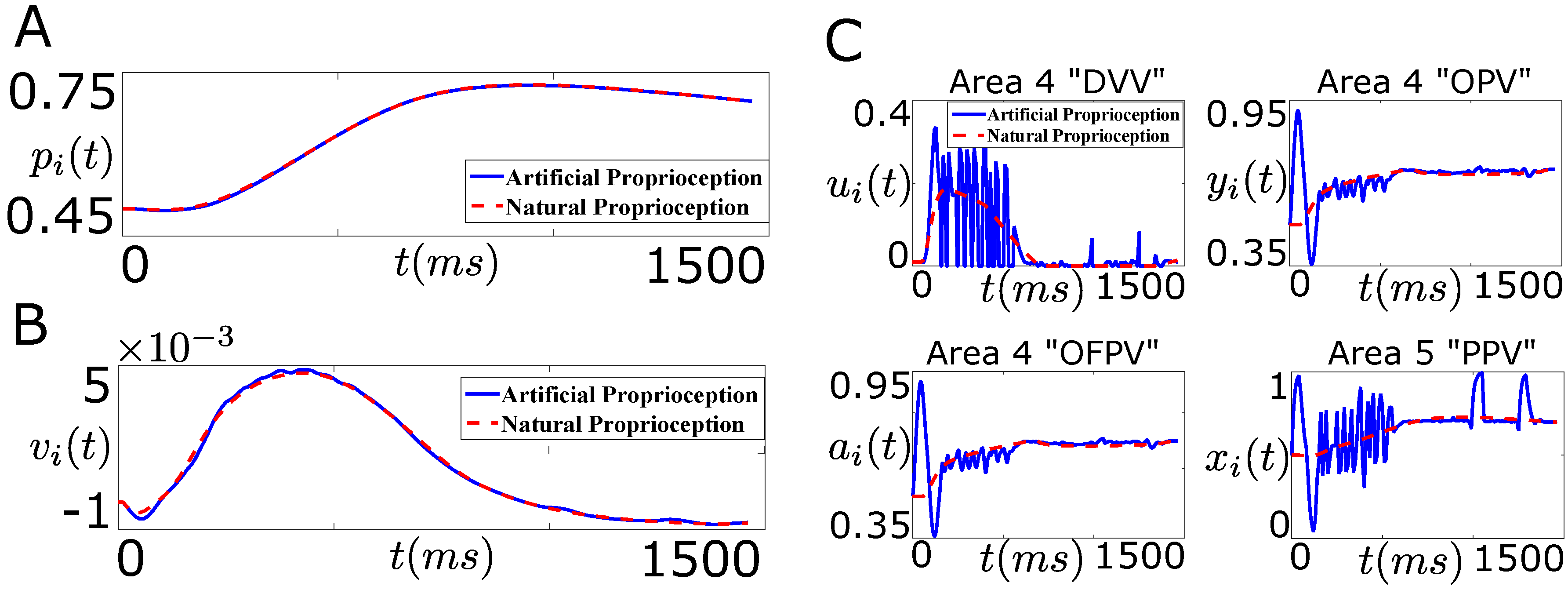
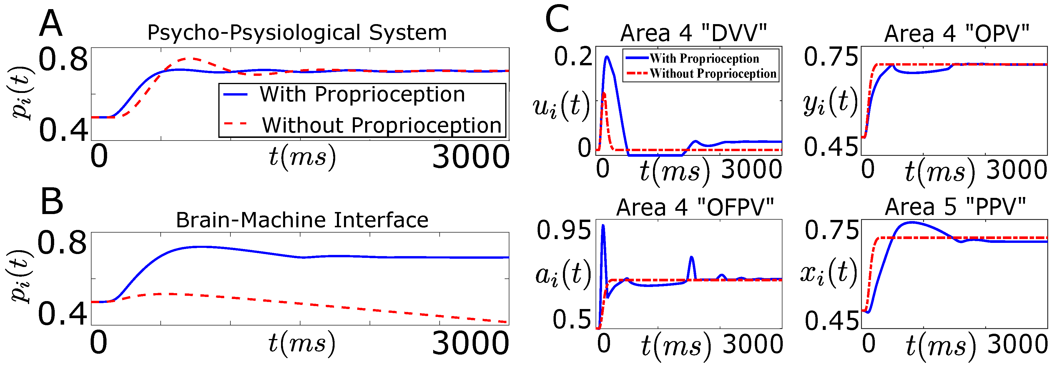
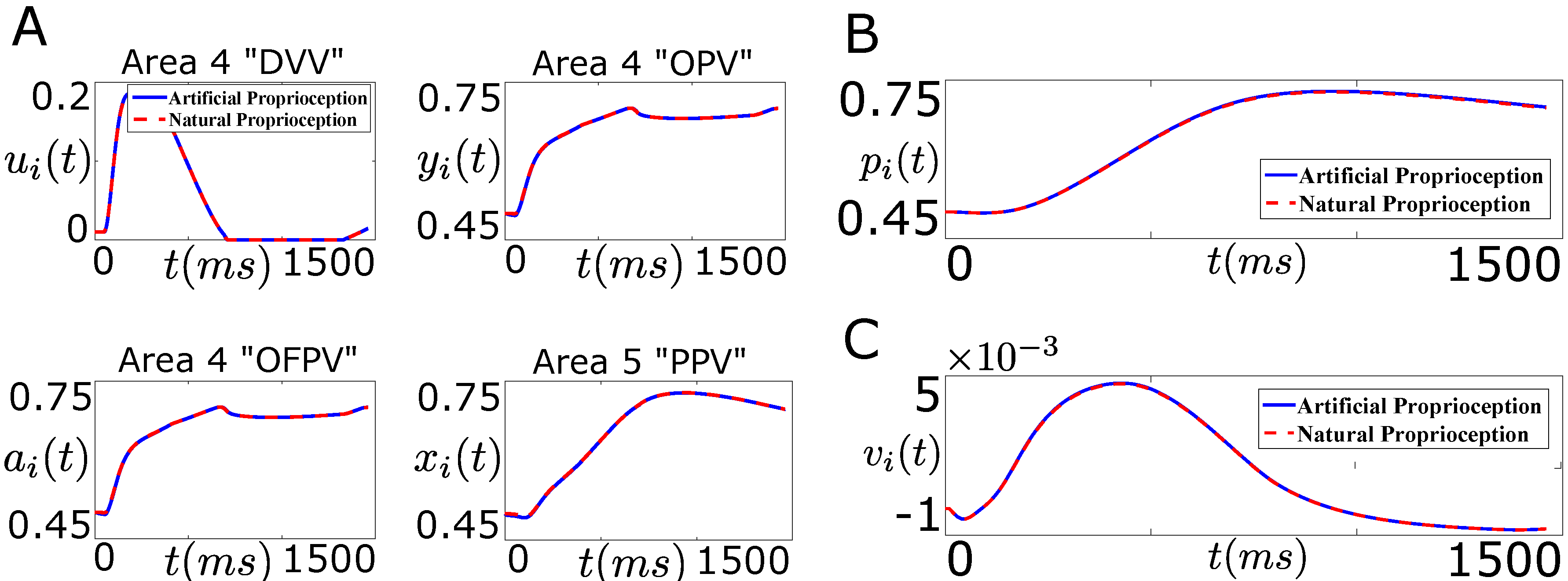
7.1. Tracking Firing Rate of Neurons which Encode Sensory Information Recovers the Natural Performance of BMI

In this article, we have designed optimal artificial sensory feedback in a control-theoretic framework to recover the closed-loop performance of a brain-machine interface (BMI) during voluntary single joint extension task. This is the first systematic attempt to incorporate artificial proprioception in BMIs towards stimulation enhanced next generation BMIs. Our approach differs from recent closed-loop BMI system modeling approaches where the focus has mainly been on the analysis of closed-loop BMIs within optimal feedback control framework [17,18]. Two control problems, namely, the position trajectory tracking problem and the cortical sensory neurons average firing rate tracking problem, have been investigated towards designing an optimal artificial sensory feedback for the BMI in the receding horizon control framework. Our position trajectory tracking problem designs the artificial proprioceptive feedback which differs from the natural proprioceptive feedback and can potentially be learned by the BMI user as shown in [3,15]. The cortical sensory neurons average firing rate tracking problem designs the natural proprioceptive feedback through external stimulations [14]. Our results shows that tracking the natural firing activity of the cortical sensory neurons using an external stimulating controller is the appropriate approach towards recovering the natural performance of the motor task. Such an approach requires a complete understanding of how our brain encodes the sensory information. In the absence of a complete understanding of neural encoding, the position trajectory problem provides a more practical way to incorporate artificial sensory feedback in BMIs and thus to close the BMI-loop as also recognized in [15].

7.2. Generalization beyond Tracking Problems

We formulated trajectory tracking control problems to design optimal artificial sensory feedback wherein we assumed that the desired trajectory (position or firing rate) is known. Obtaining such an information a priori may not be feasible in BMI motor tasks. Nevertheless, our proposed framework, based on optimal feedback control, can be generalized to design the necessary sensory feedback and thus close the BMI-loop using the available information such as the desired end-point of the arm effector and various realistic constraints. For example, one can formulate a control problem in the model predictive control framework to minimize the error between the current position and the desired position along with penalizing the derivative of the total force to stabilize the position while ensuring the smoothness of the movement. Such control problems within the optimal control framework have been studied in the context of sensorimotor control [18,41].

7.3. Limitations

In this article, we used an experimentally validated psycho-neurophysiological cortical circuit model of a single joint extension/flexion task to design a BMI. The model provided a basis to investigate the role of proprioceptive feedback in single joint tasks and to design optimal artificial sensory feedback in a BMI using the model predictive control framework. However, this model limited our investigation to a single sensory modality as it does not include visual feedback and learning. For example, we have not investigated how our design will get affected in the presence of visual feedback and any form of cortical learning of a motor task. Since our designed controller is adaptive in nature, the designed artificial sensory feedback will adapt with the learning. It may also be possible that the design controller can help in the initial learning of the BMI task by guiding the movement and thus can reduce the learning effort of the motor task.

References

1. Nicolelis, M.A.L.; Lebedev, M.A. Principles of neural ensemble physiology underlying the operation of brain-machine interfaces. Nat. Rev. 2009, 10, 530–540. [Google Scholar] [CrossRef] [PubMed]
2. Moritz, C.T.; Perlmutter, S.I.; Fetz, E.E. Direct control of paralyzed muscles by cortical neurons. Nature 2008, 486, 639–643. [Google Scholar] [CrossRef] [PubMed]
3. Doherty, J.E.; Lebedev, M.A.; Ifft, P.J.; Zhuang, K.Z.; Shokur, S.; Bleuler, H.; Nicolelis, M.A.L. Active tactile exploration using a brain-machine-brain interface. Nature 2011, 479, 228–231. [Google Scholar] [CrossRef] [PubMed]
4. Hochberg, L.R.; Serruya, M.D.; Friehs, G.M.; Mukand, J.A.; Saleh, M.; Caplan, A.H.; Branner, A.; Chen, D.; Penn, R.D.; Donoghue, J.P. Neuronal ensemble control of prosthetic devices by a human with tetraplegia. Nature 2006, 442, 164–171. [Google Scholar] [CrossRef] [PubMed]
5. Velliste, M.; Perel, S.; Spalding, M.C.; Whitford, A.S.; Schwartz, A.B. Cortical control of a prosthetic arm for self-feeding. Nature 2008, 453, 1098–1101. [Google Scholar] [CrossRef] [PubMed]
6. Koyoma, S.; Chase, S.M.; Whitford, A.S.; Velliste, M.; Schwartz, A.B.; Kass, R.E. Comparison of brain-computer interface decoding algorithms in open-loop and closed-loop control. J. Comput. Neurosci. 2010, 29, 73–87. [Google Scholar] [CrossRef] [PubMed]
7. Héliot, R.; Ganguly, K.; Jimenez, J.; Carmena, J.M. Learning in closed-loop brain–machine interfaces: Modeling and experimental validation. IEEE Trans. Syst. Man Cybern. Part B Cybern. 2010, 40, 1387–1397. [Google Scholar] [CrossRef] [PubMed]
8. Cunnigham, J.P.; Nuyujukian, P.; Gilja, V.; Chestek, C.A.; Ryu, S.I.; Shenoy, K.V. A closed-loop human simulator for investigating the role of feedback-control in Brain Machine Interfaces. J. Neurophysiol. 2011, 105, 1932–1949. [Google Scholar] [CrossRef] [PubMed]
9. Moritz, C.T.; Fetz, E.E. Volitional control of single cortical neurons in a brain-machine interface. J. Neural Eng. 2011, 8, 025017. [Google Scholar] [CrossRef] [PubMed]
10. Hochberg, L.R.; Bacher, D.; Jarosiewicz, B.; Masse, N.Y.; Simeral, J.D.; Vogel, J.; Haddadin, S.; Liu, J.; Cash, S.S.; van der Smagt, P.; et al. Reach and grasp by people with tetraplegia using a neurally controlled robotic arm. Nature 2012, 485, 372–375. [Google Scholar] [CrossRef] [PubMed]
11. Ethier, C.; Oby, E.R.; Bauman, M.J.; Miller, L.E. Restoration of grasp following paralysis through brain-controlled stimulation of muscles. Nature 2012, 485, 368–371. [Google Scholar] [CrossRef] [PubMed]
12. Scherberger, H. Neural control of motor prostheses. Curr. Opin. Neurobiol. 2009, 19, 629–633. [Google Scholar] [CrossRef] [PubMed]
13. Suminski, A.J.; Tkach, D.C.; Fagg, A.H.; Hatsopoulos, N.G. Incorporating feedback from multiple sensory modalities enhances brain-machine interface control. J. Neurosci. 2010, 30, 16777–16787. [Google Scholar] [CrossRef] [PubMed]
14. Weber, D.J.; London, B.M.; Hokanson, J.A.; Ayers, C.A.; Gaunt, R.A.; Torres, R.R.; Zaaimi, B.; Miller, L.E. Limb-state information encoded by peripheral and central somatosensory neurons: Implications for an afferent interface. IEEE Trans. Neural Syst. Rehabil. Eng. 2011, 19, 501–513. [Google Scholar] [CrossRef] [PubMed]
15. Dadarlat, M.C.; O’Doherty, J.E.; Sabes, P.N. A learning-based approach to artificial sensory feedback leads to optimal integration. Nat. Neurosci. 2015, 18, 138–144. [Google Scholar] [CrossRef] [PubMed]
16. Kumar, G.; Aggarwal, V.; Thakor, N.V.; Schieber, M.H.; Kothare, M.V. An optimal control problem in closed-loop neuroprostheses. In Proceedings of the 2011 50th IEEE Conference on Decision and Control and European Control Conference (CDC-ECC), Orlando, FL, USA, 12–15 December 2011; pp. 53–58.
17. Lagang, M.; Srinivasan, L. Stochastic optimal control as a theory of brain-machine interface operation. Neural Comput. 2013, 25, 374–417. [Google Scholar] [CrossRef] [PubMed]
18. Benyamini, M.; Zacksenhouse, M. Optimal feedback control successfully explains changes in neural modulations during experiments with brain-machine interfaces. Front. Syst. Neurosci. 2015, 9, 71. [Google Scholar] [CrossRef] [PubMed]
19. Kumar, G.; Schieber, M.H.; Thakor, N.V.; Kothare, M.V. Designing closed-loop brain-machine interfaces using optimal receding horizon control. In Proceedings of the 2013 American Control Conference, Washington, DC, USA, 17–19 June 2013; pp. 5029–5034.
20. Pan, H.; Ding, B.; Zhong, W.; Kumar, G.; Kothare, M.V. Designing Closed-loop Brain-Machine Interfaces with Network of Spiking Neurons Using MPC Strategy. In Proceedings of the 2015 American Control Conference, Chicago, IL, USA, 1–3 July 2015; pp. 2543–2548.
21. Bullock, D.; Cisek, P.; Grossberg, S. Cortical Networks for Control of Voluntary Arm Movements under Variable Force Conditions. Cerebral Cortex 1998, 8, 48–62. [Google Scholar] [CrossRef] [PubMed]
22. Kim, S.P.; Sanchez, J.C.; Rao, Y.N.; Erdogmus, D.; Carmena, J.M.; Lebedev, M.A.; Nicolelis, M.A.L.; Principe, J.C. A comparison of optimal MIMO linear and nonlinear models for brain-machine interfaces. J. Neural Eng. 2006, 3, 145–161. [Google Scholar] [CrossRef] [PubMed]
23. Wu, W.; Mumford, D.; Gao, Y.; Bienenstock, E.; Donoghue, J.P. Modeling and decoding motor cortical activity using a switching Kalman filter. IEEE Trans. Biomed. Eng. 2004, 51, 933–942. [Google Scholar] [CrossRef] [PubMed]
24. Wu, W.; Black, M.J.; Mumford, D.; Gao, Y.; Bienenstock, E.; Donoghue, J.P. Bayesian population decoding of motor cortical activity using a Kalman filter. Neural Comput. 2006, 18, 80–118. [Google Scholar] [CrossRef] [PubMed]
25. Mulliken, G.H.; Musallam, S.; Anderson, R.A. Decoding trajectories from posterior parietal cortex ensembles. J. Neurosci. 2008, 28, 12913–12926. [Google Scholar] [CrossRef] [PubMed]
26. Li, Z.; O’Doherty, J.E.; Hanson, T.L.; Lebedev, M.A.; Henriquez, C.S.; Nicolelis, M.A.L. Unscented Kalman Filter for Brain-Machine Interfaces. PLoS ONE 2009, 4, e6243. [Google Scholar] [CrossRef] [PubMed]
27. Dangi, S.; Gowda, S.; Héliot, R.; Carmena, J.M. Adaptive Kalman filtering for closed-loop Brain-Machine Interface systems. In Proceedings of the 2011 5th International IEEE/EMBS Conference on Neural Engineering (NER), Cancun, Mexico, 27 April–1 May 2011; pp. 609–612.
28. Gilja, V.; Nuyujukian, P.; Chestek, C.A.; Cunningham, J.P.; Yu, B.M.; Fan, J.M.; Churchland, M.K.; Kaufman, M.T.; Kao, J.C.; Ryu, S.I.; et al. A high-performance neural prosthesis enabled by control algorithm design. Nature Neurosci. 2012, 15, 1752–1757. [Google Scholar] [CrossRef] [PubMed]
29. Aggarwal, V.; Acharya, S.; Tenore, F.; Shin, H.C.; Cummings, R.E.; Schieber, M.H.; Thakor, N.V. Asynchronous decoding of dexterous finger movements using M1 neurons. IEEE Trans. Neural Syst. Rehabil. Eng. 2008, 16, 3–14. [Google Scholar] [CrossRef] [PubMed]
30. Sussillo, D.; Nuyujukian, P.; Fan, J.M.; Kao, J.C.; Stavisky, S.D.; Ryu, S.I.; Shenoy, K.V. A recurrent neural networks for closed-loop intracortical brain-machine interface decoders. J. Neural Eng. 2012, 9, 026027. [Google Scholar] [CrossRef] [PubMed]
31. Bizzi, E.; Accornero, N.; Chapple, W.; Hogan, W. Posture control and trajectory formation during arm movement. J. Neurosci. 1984, 4, 2738–2744. [Google Scholar] [PubMed]
32. Hanson, T.L.; Omarsson, B.; O’Doherty, J.E.; Peikon, I.A.; Lebedev, M.A.; Nicolelis, M.A.L. High-side digitally current controlled biphasic bipolar microstimulator. IEEE Trans. Neural Syst. Rehabil. Eng. 2012, 20, 331–340. [Google Scholar] [CrossRef] [PubMed]
33. Gerstner, W.; Kistler, W.M. Spiking Neuron Models: Single Neurons, Populations, Plasticity; Cambridge University Press: Cambridge, UK, 2002. [Google Scholar]
34. Merrill, D.R.; Bikson, M.; Jeffreys, J.G.R. Electrical stimulation of excitation tissue: Design of efficacious and safe protocols. J. Neurosci. Methods 2005, 141, 171–198. [Google Scholar] [CrossRef] [PubMed]
35. Davidovics, N.S.; Fridman, G.Y.; Chiang, B.; Santina, C.C.D. Effects of biphasic current pulse frequency, amplitude, duration, and interphase gap on eye movement responses to prosthetic electrical stimulation of the vestibular nerve. IEEE Trans. Neural Syst. Rehabil. Eng. 2011, 19, 84–94. [Google Scholar] [CrossRef] [PubMed]
36. Cogan, S. Neural stimulation and recording electrodes. Annu. Rev. Biomed. Eng. 2008, 10, 275–309. [Google Scholar] [CrossRef] [PubMed]
37. Rakos, M.; Freudenschuss, B.; Girsch, W.; Hofer, C.; Kaus, J.; Meiners, T.; Paternostro, T.; Mayr, W. Electromyogram-controlled functional electrical stimulation for treatment of the paralyzed upper extremity. Artif. Organs 1999, 23, 466–469. [Google Scholar] [CrossRef] [PubMed]
38. Micera, S.; Keller, T.; Lawrence, M.; Morari, M.; Popovic, D.B. Wearable neural prostheses. IEEE Eng. Med. Biol. Mag. 2010, 29, 64–69. [Google Scholar] [CrossRef] [PubMed]
39. Butson, C.R.; McIntyre, C.C. Differences among implanted pulse generator waveforms cause variations in the neural response to deep brain stimulation. Clin. Neurophysiol. 2007, 118, 1889–1894. [Google Scholar] [CrossRef] [PubMed]
40. Watanabe, T.; Kikuchi, H.; Fukushima, T.; Tomita, H.; Sugano, E.; Kurino, H.; Tanaka, T.; Tamai, M.; Koyanagi, M. Novel retinal prosthesis system with three dimensionally stacked LSI chip. In Proceedings of the 36th European Solid-State Device Research Conference, Montreux, Switzerland, 19–21 September 2006; pp. 327–330.
41. Todorov, E. Optimality principles in sensorimotor control. Nat. Neurosci. 2004, 7, 907–915. [Google Scholar] [CrossRef] [PubMed]
42. Bratton, D.; Kennedy, J. Defining a standard for particle swarm optimization. In Proceedings of the Swarm Intelligence Symposium, Honolulu, HI, USA, 1–5 April 2007; pp. 120–127.
43. Wei-Min, Z.; Shao-Jun, L.; Feng, Q. θ-PSO: A new strategy of particle swarm optimization. J. Zhejiang Univ. Sci. A 2008, 9, 786–790. [Google Scholar] [CrossRef]
44. Shi, Y.; Eberhart, R. A modified particle swarm optimizer. In Proceedings of the 1998 IEEE International Conference on Evolutionary Computation, IEEE World Congress on Computational Intelligence, Anchorage, AK, USA, 4–9 May 1998; pp. 69–73.
Figure 1. A closed-loop brain-machine interface (BMI).
Technologies 04 00018 g001
Figure 2. A psycho-physiological cortical circuit model for voluntary control of single joint movement: The diagram has been redrawn from Bullock et al. [21], Figure 1 . 1 . Nomenclature (adopted from [21]): “GO” is a scalable gating signal; “DVV” is the desired velocity vector; “OPV” is the outflow position vector; “OFPV” is the outflow force and position vector; “SFV” is the static force vector; “IFV” is the inertial force vector; “PPV” is the perceived position vector; “DV” is the difference vector; “TPV” is the target position vector; “ γ d ” and “ γ s ” are dynamic and static gamma motoneurons respectively; “α” is alpha motoneuron; “ I a ” and “ I I ” are type Ia and II afferent fibers; − represents inhibitory feedback. The rest of the connections are excitatory.
Technologies 04 00018 g002
Figure 3. Comparison of the offline performances of the Wiener filter and the Kalman filter based decoders for the single joint reaching task on a sample part of the test data. (A,C,E) show the comparison between the experimental (dotted line, red) and the decoded (solid line, blue) joint position p i ( k ) , joint velocity, v i ( k ) and force difference between the agonist and the corresponding antagonist muscle, Δ M ( k ) respectively for the Wiener filter based decoder; (B,D,F) show the comparison between the experimental (dotted line, red) and the decoded (solid line, blue) joint position p i ( k ) , joint velocity, v i ( k ) and force difference between the agonist and the corresponding antagonist muscle, Δ M ( k ) respectively for the Kalman filter based decoder.
Technologies 04 00018 g003
Figure 4. An open-loop BMI system design.
Technologies 04 00018 g004
Figure 5. Comparison of the open-loop performances of the Wiener filter based decoder and the Kalman filter based decoder with the performance of the closed-loop real system shown in Figure 2. (A) compares the open-loop decoder performance and the performance of the closed-loop real system when the extracted information from both decoders was the joint position, p i ( t ) ; (B) shows the open-loop decoder performance and the performance of the closed-loop real system when the extracted information from both decoders was the joint velocity, v i ( t ) ; (C) compares the open-loop decoder performance and the performance of the closed-loop real system when the extracted information from both decoders was the force difference between the agonist and the corresponding antagonist muscle, Δ M ( t ) .
Technologies 04 00018 g005
Figure 6. A closed-loop BMI system design using the natural proprioceptive feedback information (sensory feedback).
Technologies 04 00018 g006
Figure 7. Degradation in the performance of BMI in the absence of proprioception. (A,B) show the position trajectory of the agonist muscle i ( p i ( t ) ) as a function of time (t) in the presence (solid line) and in the absence (dotted line) of the natural proprioceptive feedback information. (A) shows the position trajectory for the neurophysiological system (“Psycho-Physiological System”) while (B) shows the position trajectory for the designed BMI (“Brain-Machine Interface”). The desired position target ( T i ) for the agonist muscle i in (A,B) is 0 . 7 ; (C) shows the average firing activity of a population of agonist area 4 “DVV” ( u i ( t ) ), area 4 “OPV” ( y i ( t ) ), area 4 “OFPV” ( a i ( t ) ) and area 5 “PPV” ( x i ( t ) ) neurons in the presence (solid line) and in the absence (dotted line) of the natural proprioceptive feedback information for the designed BMI.
Technologies 04 00018 g007
Figure 8. Prediction and controller move optimality in MPC.
Technologies 04 00018 g008
Figure 9. Model Predictive Control (MPC) based closed-loop BMI for Problem 1 and Problem 2. (A) shows the design for “Problem 1”. Here the model predictive controller designs the “Artificial Feedback” to stimulate “PPV” neurons such that the system output (“Single Joint Position” trajectory) mimics the “Desired Joint Position” trajectory; (B) shows the design for “Problem 2”. Here the model predictive controller designs the “Artificial Feedback” to stimulate “PPV” neurons such that the system output (“PPV Neurons Firing Rate” ) mimics the “Desired PPV Neurons Firing Rate”.
Technologies 04 00018 g009
Figure 10. Performance of the designed closed-loop BMI in tracking the desired position trajectory (“Problem 1”, Figure 9A). (A) shows the position trajectory of the agonist muscle i in the presence of the designed artificial sensory feedback (solid line, blue) and the natural sensory feedback (dotted line, red); (B) shows the velocity trajectory of the agonist muscle i in the presence of the designed artificial sensory feedback (solid line, blue) and the natural sensory feedback (dotted line, red); (C) shows the average firing activity of a population of the cortical area 4 “DVV” neurons ( u i ( t ) ), “OPV” neurons ( y i ( t ) ), “OFPV” neurons ( a i ( t ) ), and the cortical area 5 “PPV” neurons ( x i ( t ) ) in the presence of the artificial sensory feedback (solid line, blue) and the natural sensory feedback (dotted line, red).
Technologies 04 00018 g010
Figure 11. Performance of the designed closed-loop BMI in tracking the desired firing rate trajectory (“Problem 2”, Figure 9B). (A) shows the average firing activity of the cortical area 4 “DVV” neurons ( u i ( t ) ), “OPV” neurons ( y i ( t ) ), “OFPV” neurons ( a i ( t ) ), and the cortical area 5 “PPV” neurons ( x i ( t ) ) in the presence of artificial sensory feedback (solid line, blue) and the natural sensory feedback (dotted line, red); (B) shows the position trajectory of the agonist muscle i ( p i ( t ) ) in the presence of artificial sensory feedback (solid line, blue) and the natural sensory feedback (dotted line, red); (C) shows the velocity trajectory of the agonist muscle i ( v i ( t ) ) in the presence of artificial sensory feedback (solid line, blue) and the natural sensory feedback (dotted line, red).
Technologies 04 00018 g011
Figure 12. Receding horizon controller based closed-loop BMI design I. Here the receding horizon controller designs the “Artificial Feedback” stimulating current in a charge-balanced biphasic waveform to stimulate “Network of Spiking Neurons” such that the system output (“Single Joint Position” trajectory) mimics the “Desired Joint Position” trajectory.
Technologies 04 00018 g012
Figure 13. Charge-balanced Intra-cortical Micro-stimulation (ICMS) current in a biphasic waveform. Here the net current 0 T I ( t ) d t = 0 for T = i = 1 4 d i .
Technologies 04 00018 g013
Figure 14. Performance of the designed closed-loop BMI in tracking the desired position trajectory (Figure 12). (A) shows the position trajectory of the agonist muscle i in the presence of the designed artificial sensory feedback (solid line, blue) and the natural sensory feedback (dotted line, red); (B) shows the velocity trajectory of the agonist muscle i in the presence of the designed artificial sensory feedback (solid line, blue) and the natural sensory feedback (dotted line, red); (C) shows the average firing activity of a population of the cortical area 4 “DVV” neurons ( u i ( t ) ), “OPV” neurons ( y i ( t ) ), “OFPV” neurons ( a i ( t ) ), and the cortical area 5 “PPV” neurons ( x i ( t ) ) in the presence of the artificial sensory feedback (solid line, blue) and the natural sensory feedback (dotted line, red); (D) Firing trajectory of the agonist and the antagonist population of the spiking network.
Technologies 04 00018 g014