Municipal Bond Pricing: A Data Driven Method


Thomson Reuters, 30, South Colonnade, London E14 5EP, UK
*
Author to whom correspondence should be addressed.
Int. J. Financial Stud. 2018, 6(3), 80; https://doi.org/10.3390/ijfs6030080
Submission received: 16 August 2018
/
Revised: 6 September 2018
/
Accepted: 7 September 2018
/
Published: 11 September 2018
Abstract
:Price evaluations of municipal bonds have traditionally been performed by human experts based on their market knowledge and trading experience. Automated evaluation is an attractive alternative providing the advantage of an objective estimation that is transparent, consistent, and scalable. In this paper, we present a statistical model to automatically estimate U.S municipal bond yields based on trade transactions and study the agreement between human evaluations and machine generated estimates. The model uses piecewise polynomials constructed using basis functions. This provides immense flexibility in capturing the wide dispersion of yields. A novel transfer learning based approach that exploits the latent hierarchical relationship of the bonds is applied to enable robust yield estimation even in the absence of adequate trade data. The Bayesian nature of our model offers a principled framework to account for uncertainty in the estimates. Our inference procedure scales well even for large data sets. We demonstrate the empirical effectiveness of our model by assessing over 100,000 active bonds and find that our estimates are in line with hand priced evaluations for a large number of bonds.
JEL Classification:
C14; G121. Introduction
Municipal bonds are debt obligations issued by states, counties, cities, and other local government units to finance their general operations and to raise revenue for developmental projects. The value of a municipal bond is typically determined by price evaluations that reflects an estimate of what the bond holder may receive in a transaction under current market conditions. Price evaluations play a central role in the analysis of municipal bond markets and are a fundamental building block to many financial tasks. For instance, investors rely on these evaluations to value their bond portfolios accurately, while issuers establish bond pricing on new issues by reviewing current values.
1.1. Motivation and Scope
Price evaluations of municipal bonds have traditionally been performed by human experts based on their intuition, informed by past developments. Human evaluators apply their trading experience and market knowledge to deduce current bond prices. While human judgement and expertise is invaluable, an automated evaluation method is preferable for several reasons. First, we can immediately publish pricing updates based on recent market activity. It is also easy to scale evaluations to a large number of bonds in a seamless manner. The objective nature of the automatic methods result in a consistent, transparent, reliable, and explainable estimation procedure.
The returns realized on holding the bonds are often characterized using yield curves which define bond yields as a function of maturity years. The yield curves are inferred from the trade transactions in the bond market. However, only a very small subset of the municipal bonds trade on a regular basis and often sufficient price information is not available to derive the yield curve. The yields of bonds with different coupons or maturities are not immediately comparable. Volatility in trade prices caused by circumstances unique to an issuer or a particular trade may unduly affect the shape of the yield curve. In summary, the fragmented, opaque, and illiquid nature of the municipal bond market in addition to substantial price variations makes it challenging to accurately calculate the yield curves.
This paper describes a statistical model to automatically estimate municipal bond yields in the presence of uncertainty. We focus purely on trade transactions observed in the financial market to compute the yield estimates rather than financial reports or material event filings. The model performance is evaluated by comparing its yield estimates to hand priced evaluations for a large number of bonds.
1.2. Method Overview
The existing techniques to algorithmically construct yield curves can be categorized broadly into two types: parametric and nonparametric approaches. Parametric approaches use a single parametric function to fit the bond yields. They produce parsimonious models (Nelson and Siegel 1987) with very few parameters, possess good asymptotical properties, and are interpretable. However, they can capture only a limited set of yield curve shapes and are often less accurate in forecasting. In contrast, nonparametric approaches (De Boor 2001) do not assume any prior functional form and can adapt to a wide array of curve shapes. A piecewise polynomial model constructed using basis functions is employed here to estimate the yield curves. This data driven approach provides the necessary flexibility to adequately model the dispersion in yields and yet is relatively easy to interpret.
A yield curve model estimated using a small number of bond trade prices tends to be unstable. To address this trade data sparsity problem, a transfer learning based method is proposed. The idea here is to group related bonds together and incorporate aggregated group level information when constructing the curves. The transfer of information from the groups to individual curves fills the knowledge gap when sufficient price information is not available, thereby enriching the model for an individual curve. The group level information also acts as a means to avoid overfitting, producing more stable models.
The above transfer learning task is framed using a Bayesian hierarchical model (Gelman and Hill 2006). The use of a hierarchical structure produces a flexible grouping of bonds. For example, we may group together bonds from the same issuer at the bottom level, followed by bonds belonging to the same sector one level above and then the bonds with the same credit rating at the top level of the hierarchy. The intuition behind this composition is that even though the issuer level yield curves may differ from each other, issuers belonging to the same sector will share some common characteristics. By accounting for both the individual level differences and the group level similarities, the resulting model is robust to small sample size. The Bayesian model allows us to capture the inter-relations between the various hierarchical levels through a prior structure. Yield curves at the top level of the hierarchy, constructed during the Bayesian inference procedure, by themselves may provide interesting insights. The Bayesian approach also offers several advantages when estimating the regression function. We can sidestep the problem of choosing the number of polynomial pieces a priori and treat them as random variables that must be inferred. Furthermore, shape constraints such as monotonicity can be enforced through appropriate priors.
The standard inference procedure in Bayesian models is Markov Chain Monte Carlo (MCMC) where samples are drawn from the target posterior distribution. Traditional MCMC methods are inefficient when sampling from distributions with a large number of parameters, as is the case with hierarchical models. Recently, Hamiltonian Monte Carlo (HMC) (Neal 2011) has gained popularity due to its ability to sample efficiently from high dimensional distributions. It exploits the geometry of the target distribution to make large jumps when sampling, thereby exploring the parameter space in a much more effective manner. An HMC-based algorithm is used here to efficiently perform posterior inference on a large dataset.
1.3. Contributions
The described model was evaluated using over 100,000 investment grade U.S municipal bonds that traded during a one year period from 13 April 2017 to 13 April 2018. We show that for more than 80% of the bonds, the yield estimates produced by our model are within only 25 basis points of hand priced evaluations. We also illustrate that the model’s ability to forecast price is comparable to that of humans. Our results demonstrate a compelling case for automation. To the best of our knowledge, this is the first industrial scale study to assess the agreement between expert human evaluations and machine generated estimates in the municipal bonds space. Our proposed model is generic in the sense that it can be extended to bond markets other than municipal bonds. This paper makes the following contributions:
- A data driven curve fitting procedure that handles a wide variety of yield curve shapes.
- A novel transfer learning method to address insufficient trade information.
- A Bayesian model averaging approach to account for model uncertainty.
- An inference mechanism that can scale well to large datasets.
- Empirical evaluations on real-world municipal bonds data.
2. Related Work
There have been several attempts in the past to model and forecast the term structure of bond yields. The attention to this task is unsurprising considering the complexity of the problem and its significance in the functioning of financial markets. A popular approach is to summarize the price information for the large number of bonds that are traded using a small number of parameters. The assumption here is that nearly all bond price information is governed by a few underlying factors and using a compact model provides stable predictions.
The Nelson and Siegel (1987) model is a simple parsimonious model that uses second-order polynomials to fit the bond yields. It is based on a mathematical class of approximating functions called the Laguerre functions which consist of a polynomial times an exponential decay term. The parameters of the model can be interpreted as measuring the strengths of the short, medium, and long term components of the yield curve. Marlowe (2015) used the Nelson–Siegel model to derive a credit risk free municipal bond yield curve using the interdealer trades of pre-refunded bonds. In Diebold and Li (2006), the term structure of government bond yields is modeled using time varying parameters of the Nelson–Siegel model. Svensson (1995) extended the Nelson–Siegel model with an additional term to increase its flexibility. Specifically, two new parameters were introduced that allowed the yield curves to have an extra hump. Andreasen et al. (2017) constructed synthetic zero-coupon bond yields for Canadian government bonds based on the Svensson model. The Svensson model is also used in Hattori and Miyake (2016) to estimate the yield curves of Japanese municipal bonds. Pooter (2007) evaluates the various extensions of Nelson–Siegel model for their ability to forecast the term structure of US treasury bonds.
The main problem with the above parametric approach is that it is too rigid. It discards the possibility of additional macroeconomic factors that may affect the structure of the yield curve. A function-based approach to constructing the yield curves is an attractive alternative. The idea here is to split the maturities into multiple segments and use a different basis function for each segment. A linear combination of these basis functions can then be used to derive the final smooth yield curve. Steeley (1991) applied a nonparametric approach using basis splines to estimate the term structure of British government fixed interest securities. Hattori and Miyake (2016) observed that the B-Spline method produced better yield estimates for municipal bonds when compared with the Svensson model. Lorenčič (2016) empirically contrasted the performance of spline based method with the parametric methods in the estimation of Austrian government bonds. Our method improves the putative B-Spline method by automatically selecting the location of the segments and introducing shape constraints on the yield curve.
Some recent efforts have applied models from the machine learning literature to understand municipal bonds data. For example, Dash et al. (2017) used a single layer Artificial Neural Network (ANN) and Support Vector Regression (SVR) to estimate the municipal bond term structure. A key problem with using such supervised learning techniques is that they require a large amount of data during training, which is difficult to obtain because most municipal bonds trade only a few times after issuance. This is reflected in the objective of above work, where only an aggregated benchmark curve is derived unlike our aim to estimate yields at individual bonds level.
There have also been attempts to explicitly incorporate certain bond characteristics to model the yields. For example, Wang et al. (2008) introduces liquidity as an additional factor to the pricing model and studies the effect of systematic liquidity risk on the yields of municipal bonds. Chun et al. (2018) regress the municipal bond yields on the Credit Default Swaps (CDS) premiums of the insurers. They discover that the liquidity component plays a dominant role in the composition of yield spread. Recently, Sherrill and Yerkes (2018) explored the impact of financial statement disclosures on the municipal bond yields. In contrast to the above works, we rely purely on the trade transactions to compute the yields.
Various elements of our curve fitting procedure such as its Bayesian nature, the use of a hierarchical structure and explicit shape constraints have been investigated in the statistics literature. The motivation for Bayesian nonparametric curve fitting can be traced to Denison et al. (1998), where the number and location of knot points that make up the curve segments were treated as random variables. Baladandayuthapani et al. (2005) estimated the regression curve using low-order basis splines with a random penalty parameter. The use of a Bayesian penalized spline avoids the knots selection issue by oversampling the number of knots and yet produces smooth curves. With standard smoothing techniques, it is difficult to capture the monotonic relationship between the input and response. Hence it is necessary to include additional constraints to restrict the shape of the curve. Such monotonicity constraints for Bayesian curve fitting have been investigated before, e.g., Neelon and Dunson (2004), and Brezger and Steiner (2008). There is also rich precedents for using hierarchical models both in the frequentist (Woltman et al. 2012) and Bayesian literature (Gelman and Hill 2006). Cruz-Marcelo et al. (2011) applied a hierarchical model to estimate the term structure of corporate bonds. The bonds from various companies are pooled together and the subject specific parameters are represented as a sample from a common shared distribution. Besides the intended application of the above works, a key difference with our work is the inference procedure. The above methods use standard MCMC techniques to draw a series of correlated samples. In contrast, we avoid the random walk behavior associated with typical MCMC algorithms and use first-order gradient information to explore the parameter space. This makes our method scalable to big datasets.
3. Model
Our statistical model is described in this section. The constrained piecewise polynomial curve fitting procedure is introduced first, followed by a discussion on the hierarchical nature of the model. Finally, the Bayesian formulation is presented. Figure 1 provides an overview of the model.
3.1. Curve Fitting
The objective in a regression problem is to estimate the functional relationship between a real-valued response variable and an input variable . Given a set of observation pairs , the regression model has the form:
where are independent and identically distributed random errors. The unknown function must be estimated from the observations and is used to predict future responses of new inputs. For example, let the inputs be maturity years of bonds and the response be corresponding bond yields. Once the function mapping the maturity years to yields is available, we can estimate the yields for unknown maturity years using this yield curve function.
The wide variations in trade data necessitates a flexible curve fitting procedure that is adaptable to the patterns in the data. Standard parametric regression methods such as polynomial regression predefine the function using a small number of unknown parameters. Although this produces a parsimonious representation, the resulting model is too restrictive and may not capture unexpected features of the data. In contrast, nonparametric regression methods make very few assumptions about the form of function and use a data driven approach to learn the shape of . This results in a flexible that is adaptable to the type of data being modeled. Here a nonparametric regression method using piecewise polynomials is employed to fit the yield curves.
Let be comprised of several lower order polynomial basis functions, each defined over a different subinterval (piece) of i.e., input points within a neighbourhood share the same functional form. These piecewise polynomial functions are joined together to produce a smooth composite function that is continuous everywhere. This definition can be written compactly as:
where each is a basis function and is an unknown coefficient parameter associated with the basis function.
Several basis functions exist. A cubic B-Spline basis function which has continuous first and second derivatives is employed here. The function is expanded into B-Spline basis functions of degree 3 constructed using a sequence of points within the range of inputs. This technique produces smooth estimates and can represent a wide range of shapes. Let there be prespecified knot points that delineate the subintervals of . B-Spline basis functions of degree can be derived recursively (De Boor 2001) starting from the corresponding B-Spline function of degree as follows:
Yield curves are generally upward-sloping i.e., bonds that mature at longer terms return higher yields than shorter term bonds. Thus a monotone relationship exists between the yields and the maturity years with the yields increasing as a function of the maturity years. The yield curves derived using the above B-Spline regression technique is not necessarily monotonic. A common approach to ensure monotone estimates is to introduce an additional post processing step in the curve fitting procedure. Instead of this ad-hoc method, incorporating the monotonic constraint directly into the regression model is desirable. Formally, we wish to constrain to be isotonic such that:
In the basis function expansion defined in (2), if the coefficients are in increasing order, then the linear combination is also increasing. Thus to ensure that is isotonic, it is sufficient to guarantee that the s are in increasing order, as shown in Brezger and Steiner (2008):
This constraint on the regression coefficients is applied here to obtain a monotonically increasing yield curve.
3.2. Hierarchical Model
Due to the illiquid nature of the municipal bond market, there are often very few trade observations available for many bonds. We may treat the individual bonds as homogeneous entities and construct a single yield curve by pooling all the bonds together. However, this aggregation completely ignores the information about individual variability. Alternatively, we could group bonds at a granular level based on their common characteristics (e.g., bonds from a same issuer belong to a group) and construct multiple yield curves, one corresponding to each group. While this accounts for variability between groups, it ignores the presence of possible shared similarities between the groups. Also, some groups (issuers) may not have adequate samples (trades) to arrive at a robust estimate.
An effective way to deal with this problem is to organize the bonds using a hierarchical structure with coarsely grouped bonds at top levels of the hierarchy and granularly grouped bonds at bottom levels of the hierarchy. We can then use a hierarchical model which allows to simultaneously capture relationships both within hierarchical levels and across hierarchical levels, thereby handling the correlations among the bond trades. A hierarchical organization is also in-line with common practices such as industry classification schemes (Bhojraj et al. 2003) where companies are separated into partitions in a coarse to fine manner and these partitions are used to secure performance benchmarks and perform financial and economic analysis.
The use of a hierarchical model also mitigates the small sample size problem. By borrowing strength from higher levels, the effects of inadequate trade samples in lower levels is minimized. Instead of a tabula rasa approach, which operates under the assumption that each yield curve must be estimated from scratch, the above transfer learning approach incorporates knowledge learned from one curve and reuses it in a related curve. The latent hierarchical relationship between the bonds is exploited to transfer knowledge between the bond yield curves.
Consider the level hierarchical organization in which the bonds grouped into the same hierarchical level have similar properties. Let the input observation be associated with a set of attributes , where denotes the index of the group at level that observation belongs to. Let the number of groups in level be and let denote the index of the group at a level . For example, we may have three levels (), with the bottom level () containing bonds from the same issuer, the next level () containing bonds from the same sector, and the top level () containing bonds with the same credit rating. A value denotes that observation belongs to sector . Following Equations (1) and (2), the response has the form:
where is the number of basis functions as before. Here a single set of basis functions is shared between all the observations. However, a different set of coefficients is used for each group at each hierarchical level. This captures the group level differences. The coefficient at level belonging to group is modeled in the following manner:
with the bottom level coefficients determined from the top level coefficients. By using the coefficients at level as outcome variables computed from a higher level coefficients, information is propagated from higher hierarchy levels to lower hierarchy levels. This makes the model resilient to inadequate data at lower levels. The presence of additional random errors for each group at each level is noteworthy. This indicates that the errors are not correlated between the hierarchical levels. In our example above with three levels, Equation (7) indicates that an issuer coefficient is a sum of its corresponding sector’s coefficient and a deviation specific to the issuer. All the issuers share the same coefficients of their corresponding sectors while they still maintain their individual differences.
3.3. Bayesian Extension
Classical regression models estimate a single optimal value for the coefficient parameters, given the observed data. There is an implicit assumption here that an accurate model has been chosen to explain the data. The modeling decision may be inaccurate in practice for a number of reasons, such as the choice of an error distribution, the functional form that relates the input variable to the response, presence of outliers, etc. With single point estimates, there is a failure to accommodate the uncertainty due to model choice and a false impression is provided that that the selected model is the only true model that explains the data.
In contrast, Bayesian analysis treats the model parameters as random variables and uses the posterior distribution of the parameters given the data as the basis of inference. By working with distributions on predictions, we can quantify the uncertainty in our estimates in a natural manner. The inevitable model mis-specification is also countered because we are now averaging over a number of models. The Bayesian way of mixing over possible subsets of a rich collection of models sidesteps model selection issues and produces models with quantifiable predictive capabilities.
Bayesian models require prior distributions to be placed over all the unknown parameters. These priors characterize our knowledge about the parameter values before observing any data. There is an assumption in Section 3.1 that the knot points partitioning the input range is prespecified. These knot points control the trade-off between the smoothness and flexibility of the regression curves. It is difficult to select the correct number and position of the knots in advance. If too many knots are selected, the resulting curve may be wiggly and overfit the data. On the other hand, if too few knots are selected, the under-parameterization may produce overly smooth curve and not accurately reflect the data. It is preferable to let the data determine the knots instead of fixing their value. To address this problem, a generously high number of knots that ensures sufficient flexibility is selected. A prior that introduces dependencies between adjacent regression coefficients is then placed. This prior uses a new parameter to control the amount of smoothness and this smoothness parameter is assigned its own hyper prior. The Bayesian inference mechanism allows for simultaneous estimation of the regression coefficients and the smoothness penalty parameter, with the data determining the extent of smoothness.
In total, there are three important a priori beliefs on the regression coefficients—(i) the adjacent dependency of the coefficients to ensure smoothness; (ii) the increasing order of the coefficients to enforce monotonicity constraint; and (iii) the hierarchical dependency of the coefficients with bottom level coefficients determined using top level coefficients. The Bayesian model encoding these prior beliefs is specified as follows.
Here denotes a univariate normal distribution with mean and variance , and is the standard indicator function. Using the vector notation and , Equation (8) is the distributional form of (6). Similarly Equations (9) and (10) are the stochastic analog of (7). The prior for the top level coefficients is shown in (9), with coefficient being determined from its adjacent coefficient . The variance parameter controls the amount of smoothness. A small value will constrain adjacent coefficients to be similar, thereby penalizing wiggly curves. Equation (10) defines the prior for the rest of the coefficients. Here the coefficient for a particular group at level depends on the coefficient of its corresponding parent group at level . This models the hierarchical relation. The indicator function in both of these equations introduces a lower bound for the coefficients, with the basis coefficient greater than or equal to the basis coefficient. The ordering of coefficients induced by this truncated distribution enforces the monotonicity constraint at all levels. In both (9) and (10), for the first coefficient , the lower bound is set simply to zero. The rest of the Equations (11) to (13) describe the zero mean Gaussian random errors. The variance parameters , , and are further assigned their own hyper priors. This avoids fixing the value of these parameters and are themselves estimated from data during the inference procedure.
Finally, the model presented so far assumes that all the observations are of equal importance. There may be situations where some observations must be treated differently from the others. For example, it is useful to consider the trade attributes of a bond such as the size of the trade, how recent the trade was, the type of the trade, etc., when modeling the yield curve. In such cases, it is necessary to weight the importance of observations and include this sample weight as part of the regression model. Let denote a positive real-valued known weight value corresponding to the input observation . The size of the weight reflects the importance of the observation. The response variable in Equation (8) is modified to include the weight term as follows.
Instead of assuming that the variance of the error is constant over all values of the input, the variances are now considered to be unequal. This reduces the influence of less important observations during parameter estimation. Note that each sample weight is relative to the weights of other samples. During prediction these weights may not be available and they can be set to a constant value.
4. Inference
The central computation problem is to estimate the posterior distribution of the model parameters from the observed data. Recall that the observed data comprises of the inputs, the hierarchical group attributes, and sample weights associated with the inputs and responses. This is written compactly as . The model parameters include the regression coefficients and the variances, written as . By using the priors and likelihood as defined in equations (9) to (14), the posterior density for the parameters is given as:
The integrations in the denominator of (15) are intractable and an approximate inference method must be applied. As is common in Bayesian inference, we shall follow Monte Carlo estimation by drawing samples that converge towards the target posterior distribution and evaluate expectations using these samples during prediction.
Conventionally, a Markov Chain Monte Carlo (MCMC) method such as Gibbs sampling or the Metropolis–Hastings algorithm is employed to generate the samples. In Gibbs sampling, a priori independence between the different parameters is assumed and conjugate priors are often used to analytically compute the posterior for subsets of parameters. With Metropolis–Hastings, a candidate proposal is made using a carefully chosen distribution and this proposal is accepted with some probability. The main disadvantage with both these methods is that they scale poorly with increasing dimension and complexity of the target distribution. Our parameter space is evidently high dimensional and the use of traditional MCMC methods will require an unacceptably long time for convergence.
The Hamiltonian Monte Carlo (HMC) algorithm (Betancourt 2017) works more efficiently when compared with conventional MCMC methods when generating samples from high dimensional distributions. HMC exploits the geometry of the neighborhoods in the density that contributes the most to expectations by using first-order gradient information. Specifically, it augments the parameter position variables with auxiliary momentum variables and updates these variables according to a discretized version of the Hamiltonian dynamics. A new parameter sample proposed using this method can be distant from the current sample and yet have a high probability of acceptance. This results in large jumps in the parameter space, thereby exploring new distant regions of interest in a much shorter duration and producing diffuse samples. For a dimensional parameter vector, the expected computation to draw a sample grows with Metropolis–Hastings, while it grows with HMC (Neal 2011).
The gradient based implementation of HMC (Hoffman and Gelman 2014) is employed here to sample the posterior parameters. The model gradients are analytically computed by automatic differentiation of the posterior density. Note that with this sampling approach there is no requirement to specify conjugate priors for the variance parameters. This allows to expand the scope of priors from the traditional inverse-Gamma distribution and instead specify weakly informative prior distributions that behave well for both small and large variances. In particular, we use the Half-Cauchy distribution (Polson and Scott 2012) as priors for the variance parameters which restrict them to be positive and provide weak prior knowledge. The probability density function of a Half-Cauchy distributed variable with a scale parameter is defined as:
Consequently, we have , , and as hyperparameters. The end objective is prediction, where the response for a new input must be computed. Let denote a new input and its associated hierarchical attributes. The density of response is derived as,
where are the set of posterior samples generated based on (15) and the response distribution is as defined in (8). The final predictions are constructed from averages over the samples.
5. Application
We begin this section by describing our data and explaining the steps followed to evaluate our model. We then furnish the empirical results and discuss our findings.
5.1. Data Preprocessing and Priors Setting
The transactions and terms and conditions as reported to the Municipal Securities Rulemaking Board1 (MSRB) are used to obtain trade data. In particular, trades reported for all trading days between 13 April 2017 and 13 April 2018 are considered for experiments. We use about 350,000 trades whose trade volume were greater than or equal to $750,000. Only bonds that are rated investment grade by one of the big three credit rating agencies S&P, Moody’s, and Fitch were considered. Noninvestment grade bonds and unrated bonds are excluded because they require fundamental credit analysis to arrive at meaningful price estimates. In addition, we also exclude bank qualified and pre-refunded bonds since they require a complex and subjective pricing model. Table 1 summarizes the selection criteria for bonds that are included during experiments.
During preprocessing, an outlier detection method based on studentized residuals is applied to identify trades that may unduly affect the yield computation. First, a candidate regression function is fit using a frequentist linear regression method for the trades corresponding to a group in the lower most level of the curve hierarchy. The residual error for each trade, obtained using the regression function, is then divided by an estimate of its standard deviation. Trades with a resulting residual that is greater than a threshold were excluded. We did not employ any heteroscedasticity adjustments since the squared residuals appeared uncorrelated.
As discussed in Section 3.3, each trade observation is associated with a relative weight value that encodes the importance of a trade. We consider two factors for deriving a transaction weight: the size of the trade and the date at which the trade occurred. The first weight factor is computed by scaling the trade size to a value between and with higher volume implying higher weight. Note that trades are capped at a volume of $5,000,000. Trades that occurred in the distant past were downweighted exponentially. The most recent trade receives a maximum weight of , while historical trade weights decay towards . The final sample weight is computed as a product of these two weight factors.
Following Bayesian modeling, the variance parameters themselves have Half-Cauchy hyper priors with scale hyperparameters. The scale value for (the variance corresponding to the first regression coefficient of the top level), (the observation variance at the lower most level), and (the variance corresponding to the regression coefficients of all levels except the top level) were all set to . For (the variance corresponding to the rest of the coefficients in the top level) the scale value was set to . This reduced scale value encodes our prior belief that wiggly curves must be dissuaded to avoid overfitting. We used 10 interior knot points that were uniformly spaced between 0 and 30. This proved to be sufficient to capture all variety of the yield curves. The exact choice of values for the above hyperparameters were largely immaterial. We did not discover any significant change to the results when the above values were altered, confirming the weakly informative nature of the hyper priors employed.
During inference, all the parameters are sampled from their posterior distribution. The number of sampling iterations was set to a minimum of 4000 with the number increasing for large groups. Specifically, we increased the number of iterations by 10% for every 25 additional members in the group to account for an increase in the number of parameters. Following standard practice, a large number of samples during the burn-in period were discarded, and finally only 100 samples were retained. The regression surface is then computed from the mean of the posterior samples.
5.2. Results
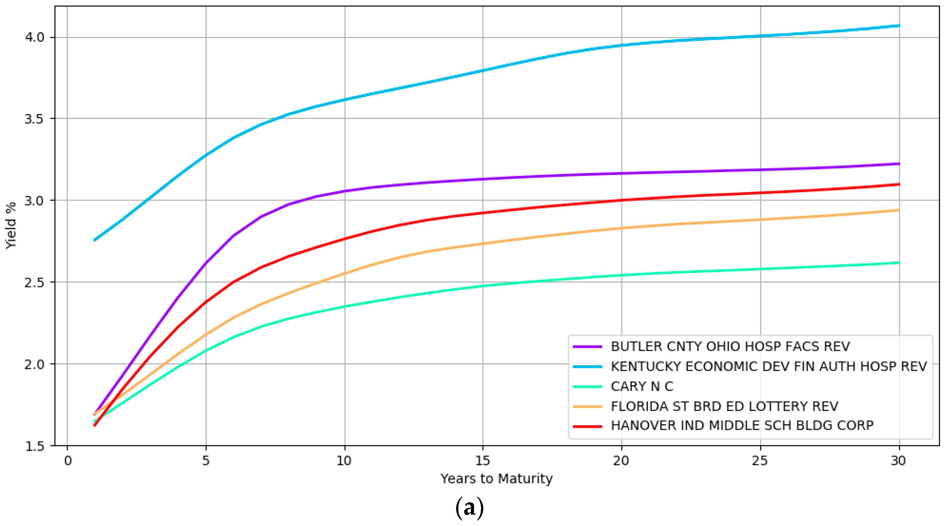
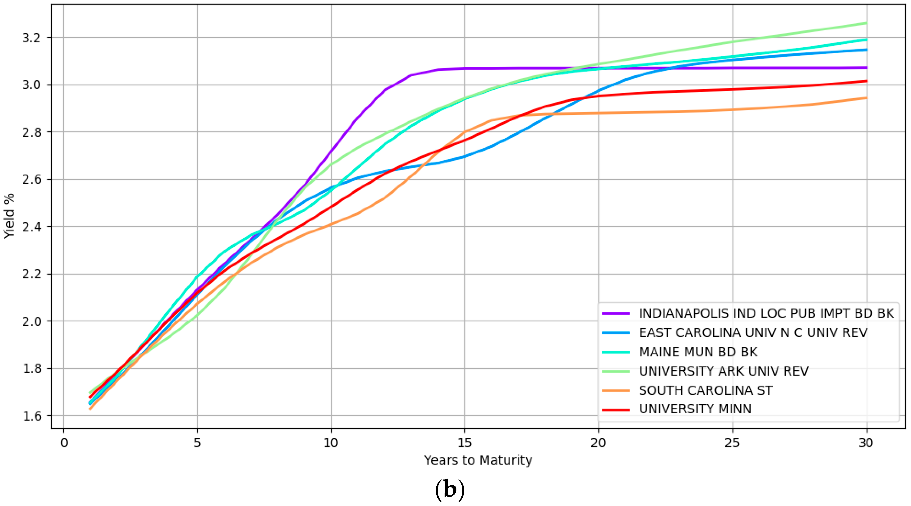
Some examples of the yield curve shapes inferred by the model at the lower most hierarchical level is presented in Figure 2. Section (a) shows the modeling of simple curve shapes such as a quadratic curve. In contrast, section (b) displays complex shapes that the model can represent.
The yield curves in this figure at section (a) correspond to five different issuers namely, BUTLER CNTY OHIO HOSP FACS REV, KENTUCKY ECONOMIC DEV FIN AUTH HOSP REV, CARY N C, FLORIDA ST BRD ED LOTTERY REV, and HANOVER IND MIDDLE SCH BLDG CORP while section (b) highlights the yield curves of six different issuers namely, INDIANAPOLIS IND LOC PUB IMPT BD BK, EAST CAROLINA UNIV NC UNIV REV, MAINE MUN BD BK, UNIVERSITY ARK UNIV REV, SOUTH CAROLINA ST, and UNIVERSITY MINN. These issuers are from different geographical locations, issue bonds of different types (e.g., general obligation and revenue bonds) and are rated differently by the credit rating agencies (e.g., the second curve in the top section is a high yield bond with BBB rating at the time of writing). The wide array of inferred curves confirms the immense flexibility that a nonparametric approach provides with both simple and complex shapes being captured depending on the heterogeneity of the data.
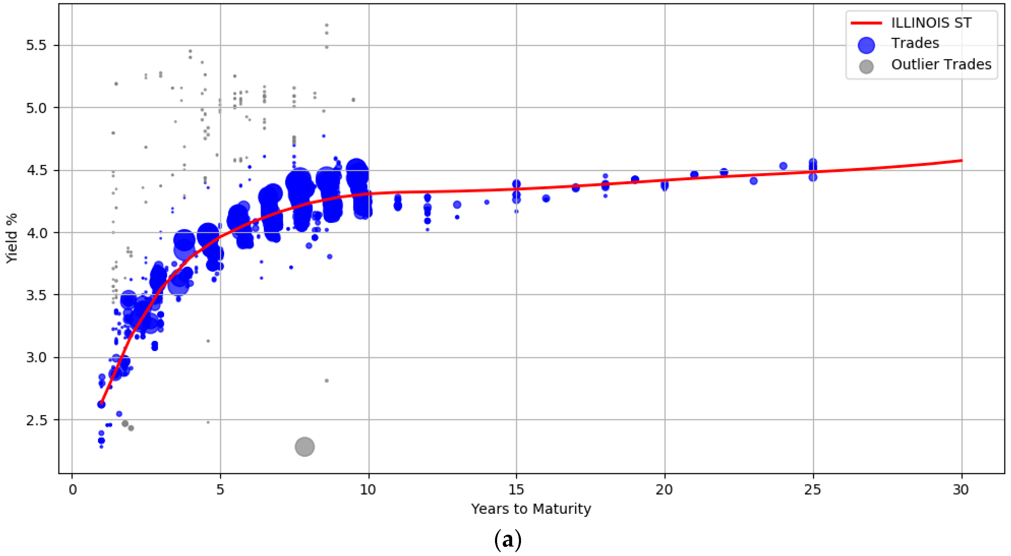
The trade information used to derive the yield curves is plotted in Figure 3. The blue circles represent the trades weighted by their attributes such as the size of the trade and the date the trade occurred. Larger circles denote points with sample weights that are relatively higher. Intuitively, the data points corresponding to small circles do not influence the yield computation as much as the data points with large circle. Section (a) shows the yield curve for the issuer ILLINOIS ST. It contains 1137 trades of general obligation bonds, all of them with a BBB credit rating. The yield curve for CONNECTICUT ST (A rated bonds) with about 480 trades is shown in section (b), while section (c) contains the curve computed from 214 trades for CLARK CNTY NEV (AA rated bonds).
The plots also show that the curves are not unduly affected by noise. There is a wide dispersion of yields for the BBB rated issuer, especially between maturity years one and ten (admittedly some of these transactions are assigned low sample weights). The prior was introduced to enforce smoothness to ensure that the curves were not overly wiggly and did not end up overfitting the data. The usefulness of the outlier detection preprocessing step can also be visualized. In all the three curves, the gray points indicate trade samples that were deemed to be abnormal and are marked as outliers.
The robustness of the model to small sample size is evident from the curves illustrated in Figure 4. Unlike Figure 3, there are very few trades available for the issuers here. The AA rated issuer CULVER CITY CALIF has only 30 trades while EL PASO CNTY TEX HOSP DIST issuer has only 18 trades. In addition, both these issuers do not have trades at the left and right boundary of the maturity years. It is clear that the unavailability of data points at the boundary did not unduly impact the curve shape.
An advantage of using the Bayesian approach is that the uncertainty in parameter estimates can be captured effectively. For example, Figure 5 shows the yield curve for issuer ESSEX CNTY N J containing approximately 40 trades. The red line corresponds to the yields computed from the mean of the posterior parameter values. The shaded region around the red line signifies the upper and lower bound of the yields when considering each individual sample of a parameter. This represents the uncertainty band around our best fit. There are no trades between maturity years 10 and 18 and the area of the shaded region here is large, depicting the greater uncertainty in our estimates.
By using the posterior distribution of the parameters, we could form credible intervals for the yield estimates during prediction. For example, when publishing the bond prices one can qualify the yield values with a certainty score that reflects the credibility of the estimates. This can be practically useful for an end user to make informed decisions. Table 2 illustrates the certainty scores associated with a few bond yields of issuer ESSEX CNTY N J. This score is a value between 0 and 1 and is calculated for each bond from a normalized difference between the upper and lower bound of the credible interval region. The bond in the first row has 1.2 years to maturity and the low certainty score is related to the width of the uncertainty band during this maturity period. This is in contrast with the bonds in the second row (maturity at 13.3 years) and third row (maturity at 7.2 years) where the width of the band narrows down. Intuitively, bonds with higher certainty scores have relatively more stable estimates than bonds with lower scores.
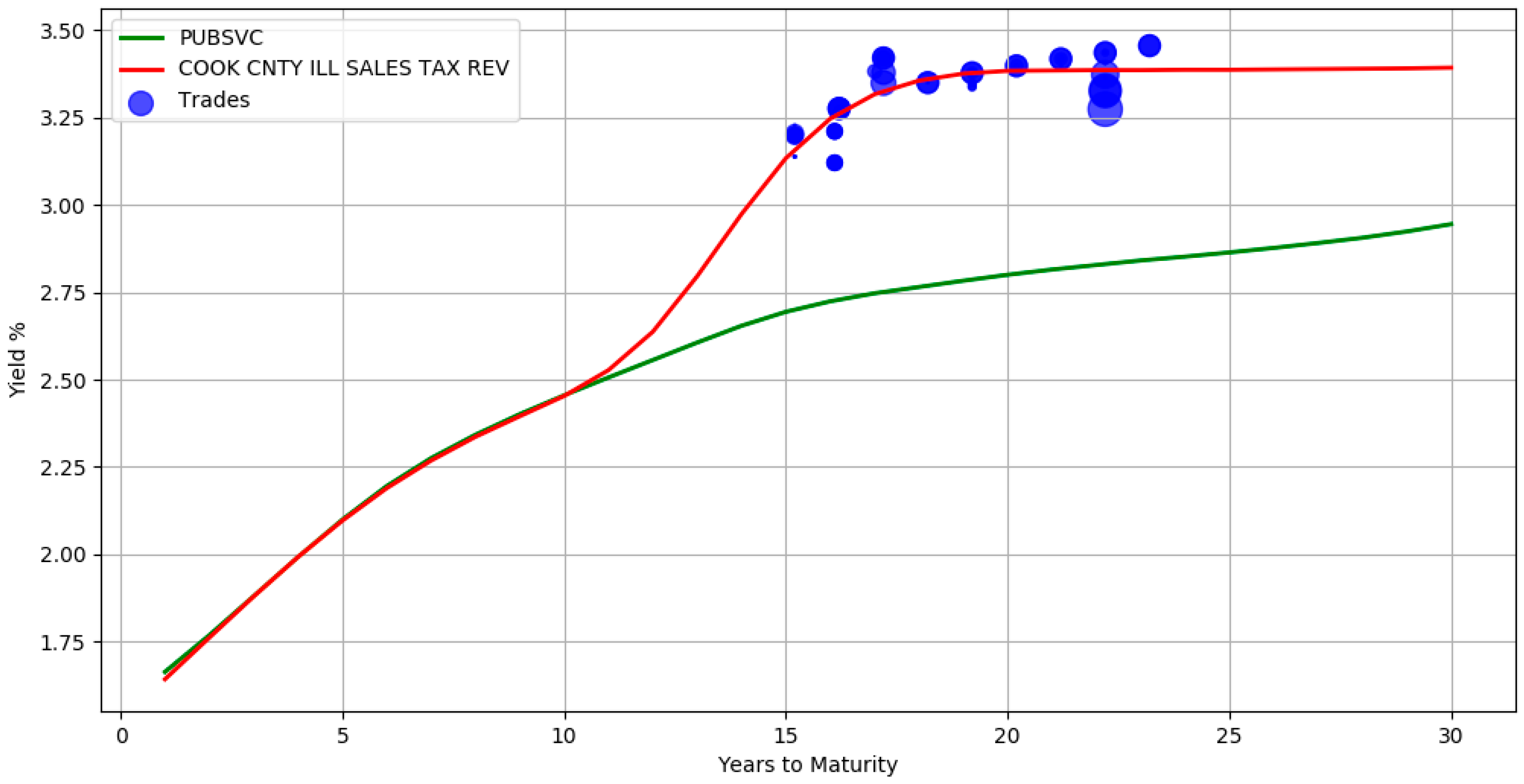
The use of a hierarchical structure allows information propagation from the top levels of the hierarchy to the bottom levels. In Figure 6, there are no trades between maturity years 1 and 15 for issuer COOK CNTY ILL SALES TAX REV. The yields during this period are inferred directly from its parent sector Public Services (the green line yield curve). It can also be seen that in the presence of adequate trade information, the bottom level red line curve deviates from its parent. This signifies that the model accounts for both the group level similarities and individual specific differences. By borrowing information from higher levels, the absence of adequate trade samples is mitigated. The above hierarchical yield curve construction procedure assumes that the actively traded bonds of the related groups is representative of the market value of an illiquid bond. While this is an approximation, it is in line with pricing practices where a basket of constituents is often used to evaluate prices.
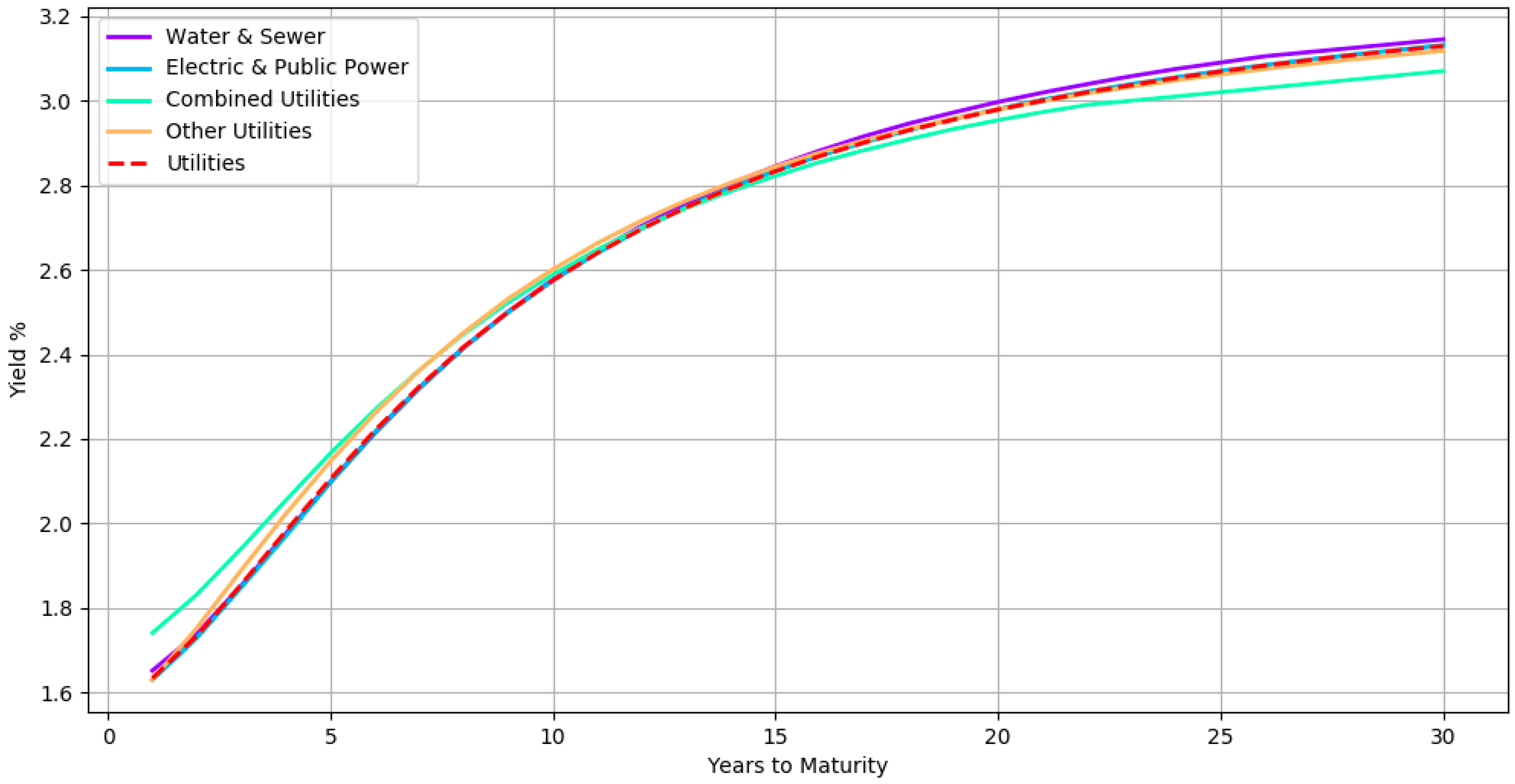
It may also be useful to visualize the curves at the various levels of hierarchy to gain insight on the latent relationship. Figure 7 shows all the subsector yield curves of a particular sector. The curves here correspond to a hierarchical organization in which bonds with the same credit rating are at the top level, followed by bonds belonging to the same sector at third level, then bonds from the same subsector at second level and finally bonds from the same issuer at the bottom level. The yield curves of subsectors Water & Sewer, Electric & Public Power, Combined Utilities, and Other Utilities are shown along with its parent sector Utilities (dashed red line) for all AA rated bonds. By inspecting the curves in the hierarchy, one can analyze how each subsector compares with its peer and its parent. For instance, the Combined Utilities subsector seems to have slightly lower yields when compared with the other subsectors.
We also compare the yields estimated by the model with the yield evaluations of human experts. The evaluations were carried out by a team of more than 20 fixed income professionals with extensive municipal bond market knowledge. The experts apply their trading experience and market contacts to arrive at an evaluated yield for the bonds every day. We considered 101,354 bonds, spanning various credit ratings, sectors, states, and bond types. A summary of the bond characteristics can be seen in Table 3. The manual evaluations correspond to price estimates as of the end-of-day on April 13 2018. The model estimates were obtained at a later date. However, the model had access to the trades only up to April 13 2018.
We used a three level hierarchical model with the bonds grouped by their credit ratings at the top level, followed by their state (for general obligation bonds) or sector (for revenue bonds) at the middle level and finally the issuer at the bottom level. Table 4 contains a breakdown of the absolute difference in yields between the human evaluators and the model estimates. It can be seen that for more than half of the bonds, the difference is less than 10 basis points. For more than 80% of the bonds, the difference is less than 25 basis points. While this difference is statistically significant, it is important to note that the model estimates are based only on trade transactions. In contrast, the human evaluators typically have access to a much more diversified pool of information sources and price recipes derived from their experience.
We also measured the difference between the model estimated yields and the actual yields observed on the next trading day. This next day trading error assesses the forecasting ability of the model. Note that not all the bonds would have traded the next day, and hence it is a subset of our universe of bonds. Table 5 displays the absolute spread between the observed yields and the model estimated yields. It also contains the spread between the next day trading yields and the yield provided by the experts. For more than half of the bonds, the model estimates perform as well as the humans’. In total, the human forecasts are within 25 basis points for 80% of the bonds while the model estimates are within 25 basis points for 72% of the bonds.
6. Conclusions
We presented a statistical model to automatically estimate the yields of municipal bonds. Our yield estimates provide essential input to a number of financial tasks such as the valuation of bond portfolios and pricing of new bond issues. By using a nonparametric model, we ensured that the functional relationship between the input and response variable was flexibly determined by the data rather than any a priori assumptions. The hierarchical organization of the bonds allowed information propagation from higher hierarchy levels to impute data gaps at lower hierarchy levels. The Bayesian nature of the model provided quantification for uncertainty in a principled manner. Our gradient based posterior sampling procedure produced an inference solution that is not limited by the sample size. Importantly, we compared our model estimates with that of human evaluators and demonstrated a compelling case for automation. In future, we intend to determine the hierarchical structure of the bonds automatically from data and extend our model by incorporating information such as financial statements and material event filings.
Author Contributions
Conceptualization, N.R.; Methodology, N.R.; Software, N.R.; Writing-Original Draft Preparation, N.R.; Writing-Review & Editing, J.L.L.; Supervision, J.L.L.
Funding
This research was funded by Thomson Reuters.
Acknowledgments
We thank the entire Thomson Reuters Municipal Bond Valuations team, particularly Daniel Chen, Afsheen Atif, Brian Lin, and Thomas Ryan for their support and contributions.
Conflicts of Interest
The authors declare no conflicts of interest.
References
- Andreasen, Martin M., Jens H. E. Christensen, and Glenn D. Rudebusch. 2017. Term Structure Analysis with Big Data. Federal Reserve Bank of San Francisco. [Google Scholar] [CrossRef]
- Baladandayuthapani, Veerabhadran, Bani K. Mallick, and Raymond J. Carroll. 2005. Spatially adaptive Bayesian penalized regression splines (P-splines). Journal of Computational and Graphical Statistics 14: 378–94. [Google Scholar] [CrossRef]
- Betancourt, Michael. 2017. A conceptual introduction to Hamiltonian Monte Carlo. arXiv preprint. arXiv:1701.02434. [Google Scholar]
- Bhojraj, Sanjeev, Charles M. C. Lee, and Derek K. Oler. 2003. What’s my line? A comparison of industry classification schemes for capital market research. Journal of Accounting Research 41: 745–74. [Google Scholar] [CrossRef]
- Boor, Carl D. 2001. A Practical Guide to Splines. New York: Springer. [Google Scholar]
- Brezger, Andreas, and Winfried J. Steiner. 2008. Monotonic Regression Based on Bayesian P–Splines: An Application to Estimating Price Response Functions from Store-Level Scanner Data. Journal of Business & Economic Statistics 26: 90–104. [Google Scholar]
- Chun, Albert L., Ethan Namvar, Xiaoxia Ye, and Fan Yu. 2018. Modeling Municipal Yields with (and without) Bond Insurance. Management Science. [Google Scholar] [CrossRef]
- Cruz-Marcelo, Alejandro, Katherine B. Ensor, and Gary L. Rosner. 2011. Estimating the term structure with a semiparametric Bayesian hierarchical model: An application to corporate bonds. Journal of the American Statistical Association 106: 387–95. [Google Scholar] [CrossRef] [PubMed]
- Dash, Gordon H., Nina Kajiji, and Domenic Vonella. 2017. The role of supervised learning in the decision process to fair trade US municipal debt. EURO Journal on Decision Processes. [Google Scholar] [CrossRef]
- Denison, D. G. T., B. K. Mallick, and A. F. M. Smith. 1998. Automatic Bayesian curve fitting. Journal of the Royal Statistical Society: Series B (Statistical Methodology) 60: 333–50. [Google Scholar] [CrossRef]
- Diebold, Francis X., and Canlin Li. 2006. Forecasting the term structure of government bond yields. Journal of Econometrics 130: 337–64. [Google Scholar] [CrossRef]
- Gelman, Andrew, and Jennifer Hill. 2006. Data Analysis Using Regression and Multilevel/Hierarchical Models. Cambridge: Cambridge University Press. [Google Scholar]
- Hattori, Takahiro, and Hiroki Miyake. 2016. The Japan Municipal Bond Yield Curve: 2002 to the Present. International Journal of Economics and Finance 8: 118. [Google Scholar] [CrossRef]
- Hoffman, Matthew D., and Andrew Gelman. 2014. The No-U-turn sampler: adaptively setting path lengths in Hamiltonian Monte Carlo. Journal of Machine Learning Research 15: 1593–623. [Google Scholar]
- Lorenčič, Eva. 2016. Testing the Performance of Cubic Splines and Nelson–Siegel Model for Estimating the Zero-coupon Yield Curve. Naše Gospodarstvo/Our Economy 62: 42–50. [Google Scholar] [CrossRef]
- Marlowe, Justin. 2015. Municipal Bonds and Infrastructure Development–Past, Present, and Future. International City/County Management Association and Government Finance Officers Association. Available online: https://www.cbd.int/financial/2017docs/usa-municipalbonds2015.pdf (accessed on 1 August 2018).
- Neal, Radford M. 2011. MCMC using Hamiltonian dynamics. In Handbook of Markov Chain Monte Carlo. Boca Raton: CRC Press. [Google Scholar]
- Neelon, Brian, and David B. Dunson. 2004. Bayesian isotonic regression and trend analysis. Biometrics 60: 398–406. [Google Scholar] [CrossRef] [PubMed]
- Nelson, Charles R., and Andrew F. Siegel. 1987. Parsimonious Modeling of Yield Curves. The Journal of Business 60: 473–89. [Google Scholar] [CrossRef]
- Polson, Nicholas G., and James G. Scott. 2012. On the half-Cauchy prior for a global scale parameter. Bayesian Analysis 7: 887–902. [Google Scholar] [CrossRef]
- Pooter, Michiel D. 2007. Examining the Nelson–Siegel Class of Term Structure Models (No. 07-043/4). Tinbergen Institute Discussion Paper. Available online: https://repub.eur.nl/pub/10219/20070434.pdf (accessed on 1 August 2018).
- Sherrill, D. E., and Rustin T. Yerkes. 2018. Municipal Disclosure Timeliness and the Cost of Debt. Financial Review 53: 51–86. [Google Scholar] [CrossRef]
- Steeley, James M. 1991. Estimating the Gilt-edged Term Structure: Basis Splines and Confidence intervals. Journal of Business Finance & Accounting 18: 513–29. [Google Scholar]
- Svensson, Lars E. 1995. Estimating Forward Interest Rates with the Extended Nelson and Siegel Method. Sveriges Riksbank Quarterly Review 3: 13–26. [Google Scholar]
- Wang, Junbo, Chunchi Wu, and Frank X. Zhang. 2008. Liquidity, default, taxes, and yields on municipal bonds. Journal of Banking & Finance 32: 1133–49. [Google Scholar]
- Woltman, Heather, Andrea Feldstain, J. C. MacKay, and Meredith Rocchi. 2012. An introduction to hierarchical linear modeling. Tutorials in Quantitative Methods for Psychology 8: 52–69. [Google Scholar] [CrossRef] [Green Version]
| 1 |
Figure 1.
Model overview using plate notation. The response is determined from the input variables and the regression coefficients at the first level. The regression coefficients have dependencies across various levels (to ensure a hierarchical relation) and dependencies with adjacent coefficients (to enforce smoothness and monotonicity). The variance variables and their hyperparameters are shown on the left and right sides.
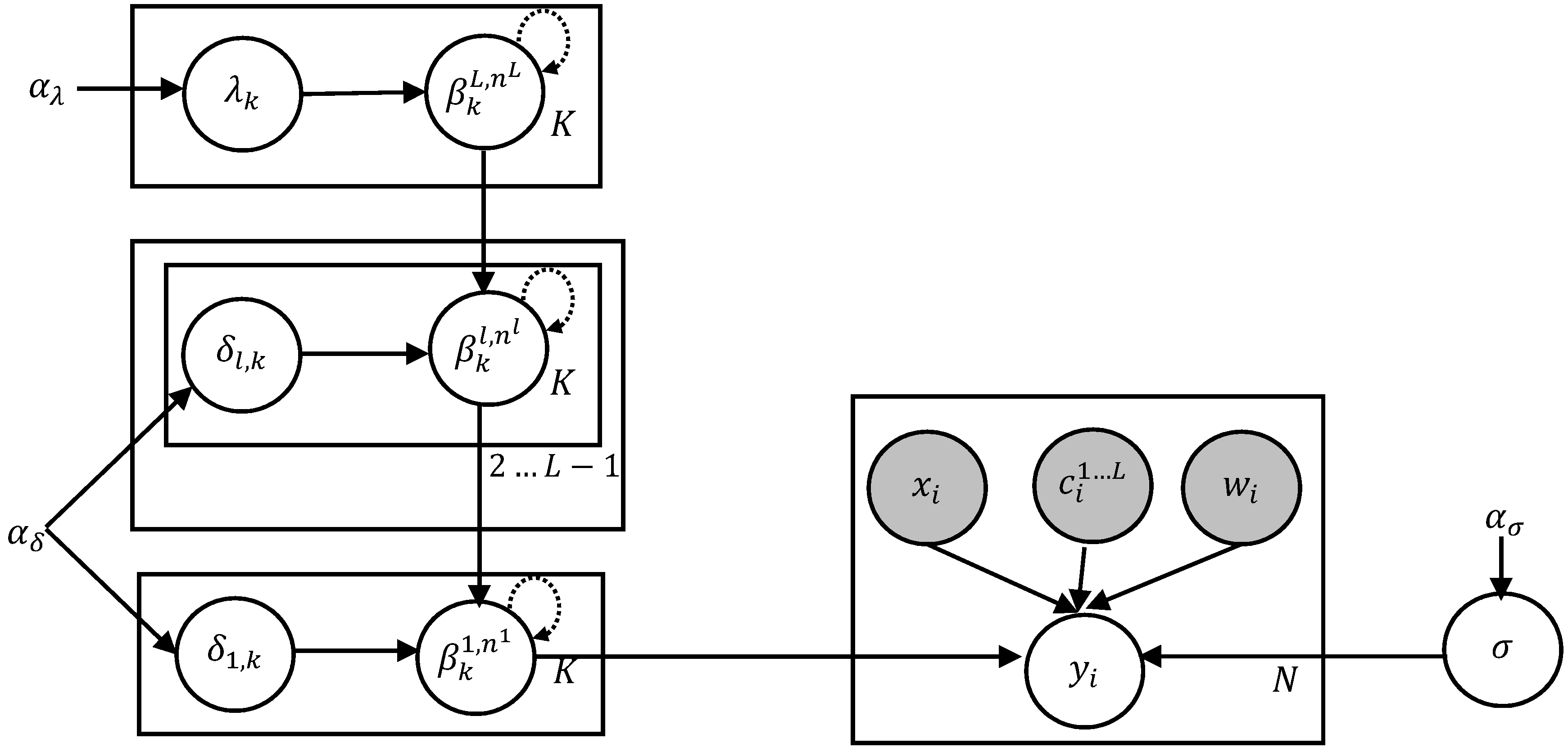
Figure 2.
Yield curve shapes inferred by the model. (a): Simple shapes such as second order polynomial curves. (b): More complex shapes. Best viewed in color.
Figure 2.
Yield curve shapes inferred by the model. (a): Simple shapes such as second order polynomial curves. (b): More complex shapes. Best viewed in color.


Figure 3.
Trade transactions and the yield curves. The circles denote the trades weighted by their attributes. The smaller the circle, the lesser a data point’s importance. (a): Illinois state. (b): Connecticut State. (c): Clark Country Nevada.
Figure 3.
Trade transactions and the yield curves. The circles denote the trades weighted by their attributes. The smaller the circle, the lesser a data point’s importance. (a): Illinois state. (b): Connecticut State. (c): Clark Country Nevada.

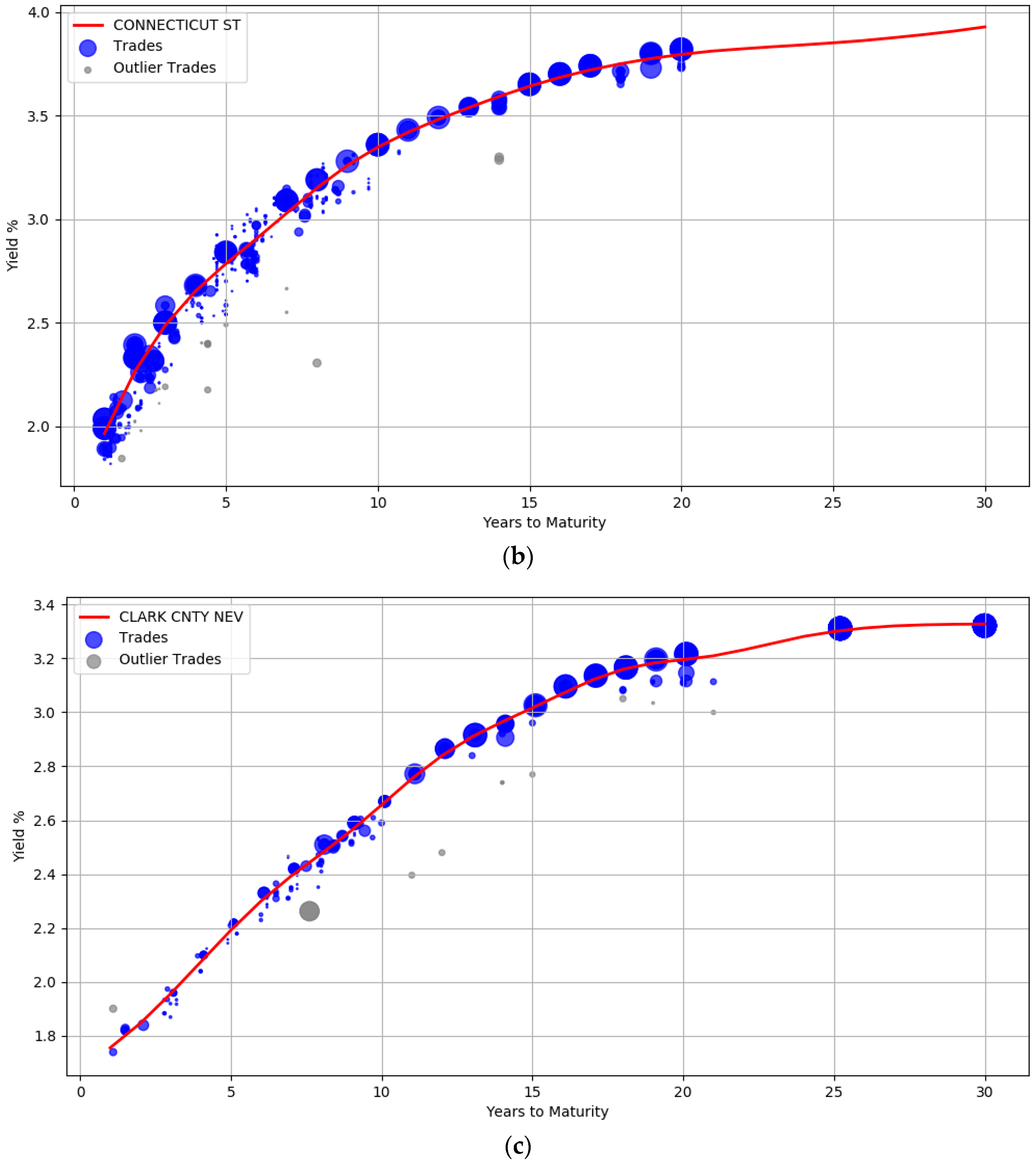
Figure 4.
Robustness to sample size. Yield curves for issuers with very few trade samples and devoid of trades at the left and right boundaries. (a): Culver City California. (b): El Paso County hospital.
Figure 4.
Robustness to sample size. Yield curves for issuers with very few trade samples and devoid of trades at the left and right boundaries. (a): Culver City California. (b): El Paso County hospital.
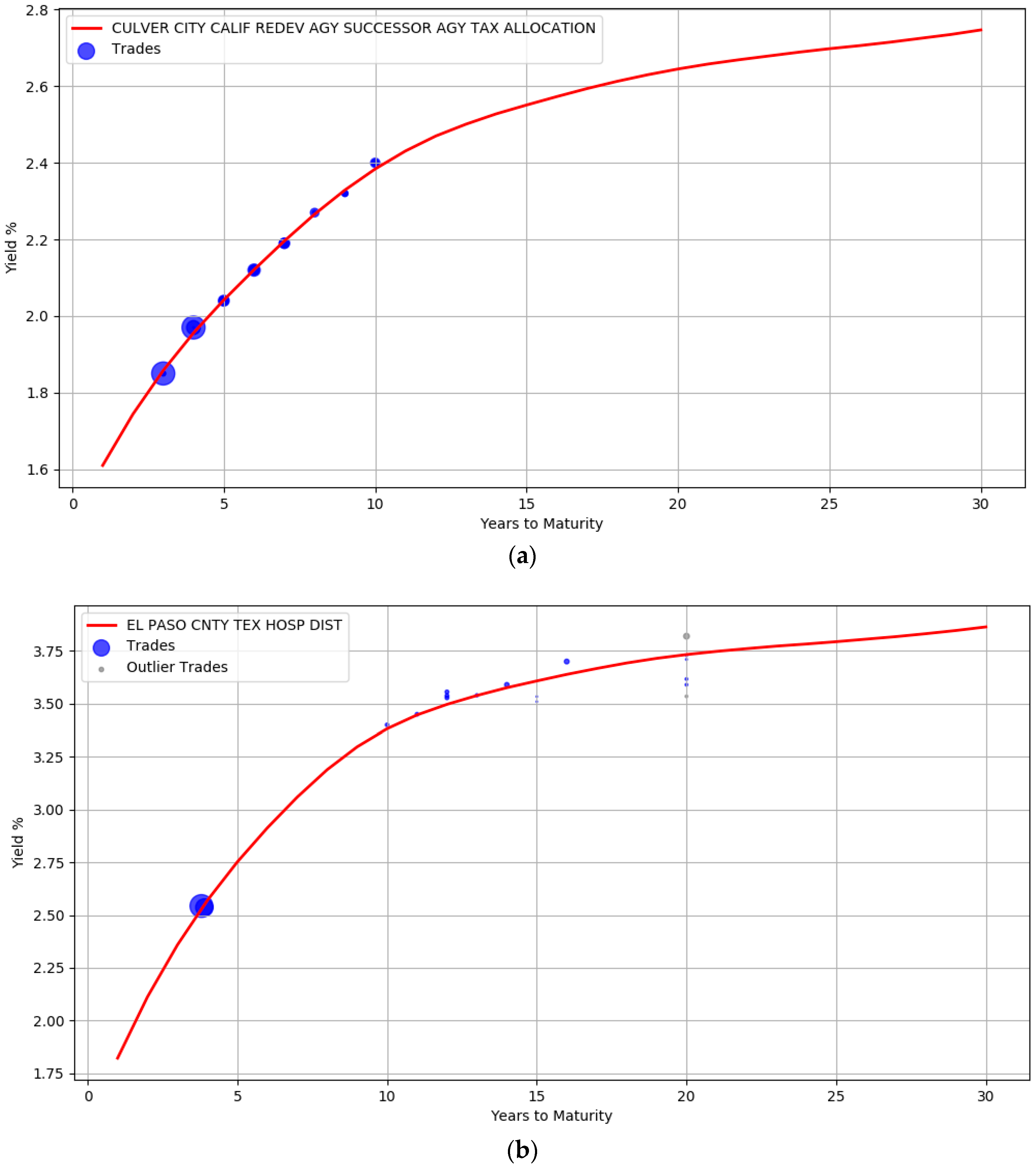
Figure 5.
Capturing uncertainty in the estimates. The shaded region represents the uncertainty band around the mean.
Figure 5.
Capturing uncertainty in the estimates. The shaded region represents the uncertainty band around the mean.
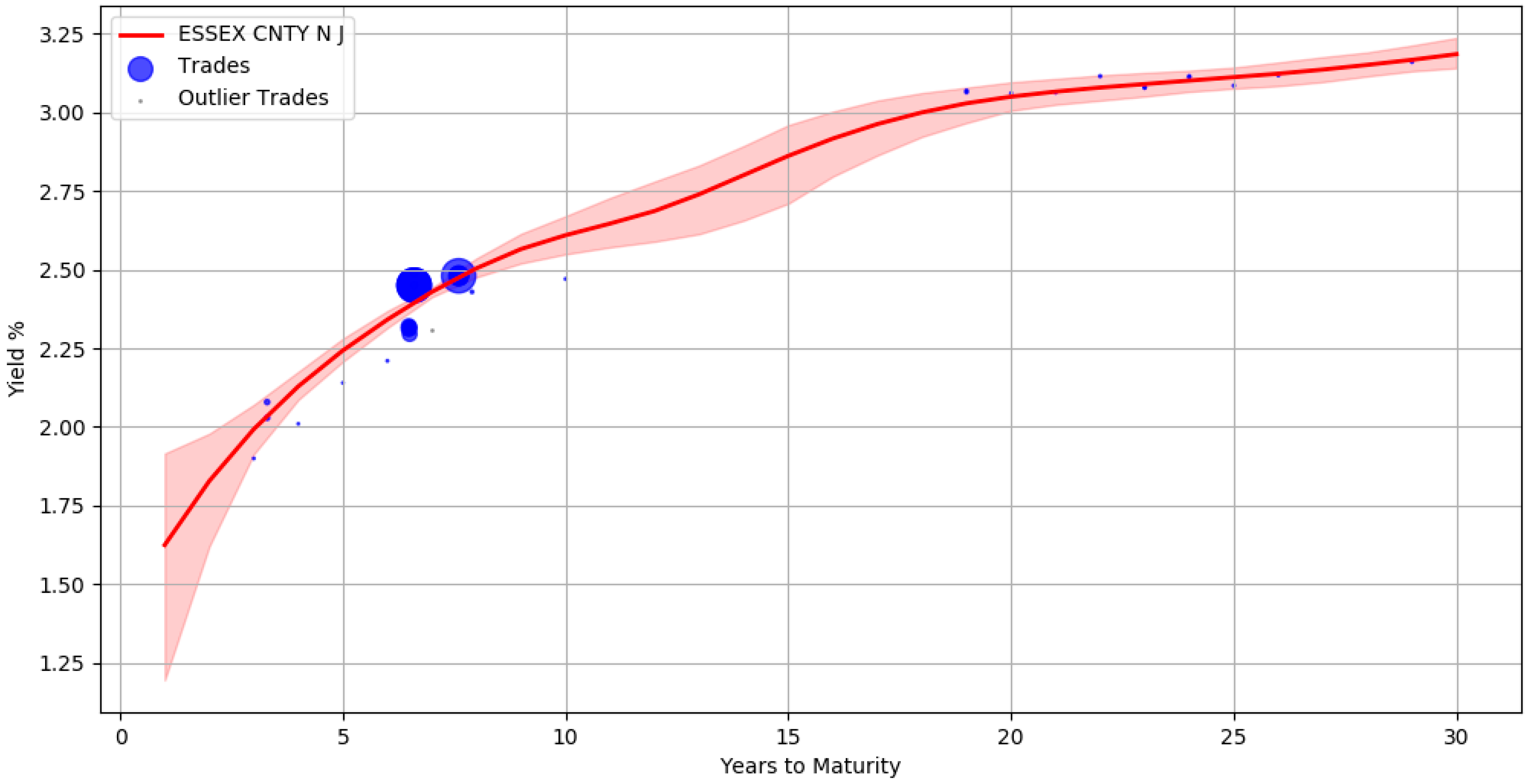
Figure 6.
Information propagation from top level to bottom level in the hierarchy. The green line corresponds to the parent yield curve.
Figure 6.
Information propagation from top level to bottom level in the hierarchy. The green line corresponds to the parent yield curve.

Figure 7.
Visualizing the latent hierarchical relationship. The red dashed line is the yield curve of a sector. The rest of the solid lines correspond to its children subsectors.
Figure 7.
Visualizing the latent hierarchical relationship. The red dashed line is the yield curve of a sector. The rest of the solid lines correspond to its children subsectors.

Table 1.
Bonds selection criteria.
| 1. | Select all bonds with an investment grade credit rating |
| 2. | Exclude bonds that are priced to PUT |
| 3. | Exclude taxable bonds |
| 4. | Exclude bank qualified bonds |
| 5. | Exclude pre-refunded bonds |
| 6. | Exclude escrowed to maturity bonds |
| 7. | Exclude bonds with insurance contract |
| 8. | Exclude short term callable bonds |
| 9. | Exclude bonds obligated to redeem before maturity |
| 10. | Exclude bonds whose maturity date is not between one and thirty years |
Table 2.
Certainty scores of bond yield estimates.
| Issuer | CUSIP | Yield Estimate | Certainty Score |
|---|---|---|---|
| ESSEX CNTY N J | 296804KC0 | 1.67% | 0.67 |
| ESSEX CNTY N J | 296804ZN0 | 2.89% | 0.91 |
| ESSEX CNTY N J | 296804C47 | 2.45% | 0.98 |
Table 3.
Summary of bonds used for evaluation.
| Type | Count |
|---|---|
| AAA Rated Bonds | 28,295 |
| AA Rated Bonds | 54,268 |
| A Rated Bonds | 16,290 |
| BBB Rated Bonds | 2501 |
| General Obligation Bonds | 45,296 |
| Revenue Bonds | 56,058 |
| Issuers | 844 |
Table 4.
Comparison between human evaluations and model estimates.
| Yield Spread between Human Evaluations and Model Estimates | Number of Bonds | Percentage of Bonds |
|---|---|---|
| <5 basis points | 33,906 | 33.45 |
| <10 basis points | 57,441 | 56.67 |
| <15 basis points | 69,974 | 69.03 |
| <20 basis points | 78,281 | 77.23 |
| <25 basis points | 83,990 | 82.86 |
| ≥25 basis points | 101,354 | 100.00 |
Table 5.
Next day trading error comparison.
| Next Day Yield Spread | Human Evaluation | Model Estimates |
|---|---|---|
| <5 basis points | 39.76% | 37.57% |
| <10 basis points | 57.13% | 54.09% |
| <15 basis points | 66.42% | 62.39% |
| <20 basis points | 75.33% | 67.33% |
| <25 basis points | 80.11% | 72.17% |
© 2018 by the authors. Licensee MDPI, Basel, Switzerland. This article is an open access article distributed under the terms and conditions of the Creative Commons Attribution (CC BY) license (http://creativecommons.org/licenses/by/4.0/).
Share and Cite
MDPI and ACS Style
Raman, N.; Leidner, J.L. Municipal Bond Pricing: A Data Driven Method. Int. J. Financial Stud. 2018, 6, 80. https://doi.org/10.3390/ijfs6030080
AMA Style
Raman N, Leidner JL. Municipal Bond Pricing: A Data Driven Method. International Journal of Financial Studies. 2018; 6(3):80. https://doi.org/10.3390/ijfs6030080
Chicago/Turabian StyleRaman, Natraj, and Jochen L. Leidner. 2018. "Municipal Bond Pricing: A Data Driven Method" International Journal of Financial Studies 6, no. 3: 80. https://doi.org/10.3390/ijfs6030080
Note that from the first issue of 2016, this journal uses article numbers instead of page numbers. See further details here.