Buy and Hold in the New Age of Stock Market Volatility: A Story about ETFs

1
School of Business, Brescia University, Owensboro, KY 42301, USA
2
Economics and Business Department, Berea College, Berea, KY 40404, USA
*
Author to whom correspondence should be addressed.
Int. J. Financial Stud. 2018, 6(3), 79; https://doi.org/10.3390/ijfs6030079
Submission received: 27 July 2018
/
Revised: 23 August 2018
/
Accepted: 5 September 2018
/
Published: 6 September 2018
Abstract
:The buy and hold stock market strategy, which gained tremendous popularity in the 1970s, may no longer be such a profitable method for accumulating wealth for the average investor in the new millennium. This paper investigates the relationship between compound return and holding period length to see how long an Exchange Traded Fund (ETF) investment must be held before a positive return on principal is 100% likely. Because the ETF is a relatively new investment vehicle that could be considered particularly well-suited to the requirements of the buy and hold strategy, we begin our investigation here. We find that the compound returns earned over a rolling holding period are much more volatile than one might assume given historic rules of thumb for average return expectations. Using monthly return data for all listed NASDAQ ETFs between their date of inception and 2015, we find it takes ten years for the average probability of a gain on principal to be over 95 percent.
1. Introduction
Since the 1970s, money managers entreated clients to “buy and hold”. The buy and hold strategy became synonymous with a conservative and reasonable approach to saving for retirement where the investor would pick stocks of value and give the investment time to grow. The basic idea, one that was encapsulated in the Efficient Market Hypothesis, is that it is really difficult to beat the market on a risk-adjusted basis year after year. Earning the market rate of return, without attempting to time the market, would provide sufficient means for a comfortable retirement. The investor could invest her life savings and sleep through the night, knowing that time was working to increase the nest egg in a positive direction.
This approach earned cachet with the baby boomers as they put their savings away for retirement. From 1970–1999, the average mean return for large company stocks was 14.9%, with a standard deviation of 15.98% (Ross et al. 2015, p. 390). So, on average, approximately 68% of the time an investor would earn between 30.9% and −1.08% on their investment. An investor would not earn more than the range yearly, but the market was making such high, positive returns, and the likelihood of a loss was fairly low, such that buy and hold provided what seemed like a relatively smart method for reaching retirement.
The exchange-traded fund (ETF) was designed in 1993 as a vehicle for index investing with the added benefit of tradability throughout the day. Unlike the popular mutual fund, ETFs operate like closed end funds, in that shares trade on the secondary market between buyer and seller and fund administrators do not create or destroy fund shares as the popularity of the fund waxes and wanes. Ultimately, a big question is whether ETF returns are better than mutual fund returns (See Chen et al. 2015; De Jong and Rhee 2008; Gastineau 2004; Toolson 2012). The ETFs tend to have lower expense ratios, but higher trading costs, so balancing these two against each other is a worthy consideration (See Angel et al. 2016; Dellva 2001). Beyond this choice, ETFs can provide an easy route for buy and hold strategies and are easily accessible on any stock trading platform.
The returns and volatility on the market over the last 15 years, however, have really called into question such complete faith in the buy and hold protocol. Between 2000 and 2013, the average mean return is significantly lower than what the typical investor was used to seeing, at 5.56%, and perhaps more significantly, the standard deviation was higher, at 19.89%. This would suggest that approximately 68% of the realized returns are likely to fall somewhere between 25.45% and −14.33%. Today, investors struggle to get the positive returns they were accustomed to, and the probability of negative returns in any given year is a lot greater. Experts see the problem. Indeed, Andrew Lo argues:
Lo’s research suggests that the nature of the market has changed over the last 25 years, as has our understanding of investor behavior (See Lo 2004, 2005, 2012; Lo and MacKinlay 1999). Big moves in the stock market make the investor’s commitment to a buy and hold strategy really difficult in a downturn. Many investors will get nervous during a market fall and will sell at exactly the wrong time. During an upturn, investors can wait too long to buy into the market, purchasing stock vehicles at their peak. The ability to accumulate wealth becomes seriously downgraded in such a market atmosphere.Buy-and-hold doesn’t work anymore … the volatility [in the market] is too significant. Almost any asset can suddenly become much more risky. Buying into a mutual fund and holding it for 10 years is no longer going to deliver the same expected return that we saw over the course of the last seven decades, simply because of the nature of financial markets and how complex it’s gotten.
At the same time, the growth and use of index funds and ETF’s as investment vehicles have skyrocketed over the same period of time. Vanguard, as part of its mutual fund business, pulled in $196 billion in investor cash flow dedicated to passive investing, on pace to beat its record from 2014 (Krouse 2015). The implications from the article are that investors continue to strongly believe in the buy and hold strategy. It thus becomes even more important to be sure that investors’ expectations for return are being met in the form of realized returns over time.
Isolating the source of the differences between expected return and realized return and investor behavior is difficult, because the causes for such discrepancies are many, including: Monetary policy, fee structures, new financial engineering, and “pick lists” by financial gurus. But perhaps a good first step for understanding the discontinuity between the average return an investor expects, and typically uses for an investment decision, and the real compound return she actually receives is to assess the likelihood of earning a positive return in today’s new, more volatile market environment using the buy and hold strategy.
In this paper we are not going to look at return as a simple arithmetic average, to the contrary, we are simply going to ask the question: How long does it take for investors to regain or maintain their principal? Due to the nature of ETF’s, we are beginning our investigation with them. We seek insight into how the timing of a purchase impacts maintenance of principal. Given the prominence of the buy and hold strategy, we would expect that the length of the holding period required for any positive return should not be long. The question is how long is long enough? If an investor enters a market or purchases an investment product at an inopportune time, how long do they have to hold the investment in order to be reasonably certain that they will have gains? In the current environment of increased market volatility, whether the buy and hold strategy is still the best strategy for risk-averse investors is a valid question to consider. Our research method utilizes an algorithm to calculate compound, realized returns for all ETFs listed on NASDAQ over a rolling holding period since the inception of each of the individual ETFs from each ETF’s start date through 2015. The data was collected by using R to combine all publicly traded ETFs via web queries to “Yahoo Finance” for each ticker by month over the available time range. We find that the average time it takes to establish a 100% chance of earning a positive return above the principal is 10 years for our sample, while the typical ETF survives in the market for approximately 6 years. That is a significant amount of time for investors schooled in the rule of thumb of 8% per year on average. Given the amount of time required for buy and hold to gain any traction, and given that there are over 1364 ETFs to select from, confidence in such a strategy can be seriously questioned.
The paper proceeds as follows: Section 2 discusses the previous literature. Section 3 details the data and the methodology we employed. Look to Section 4 for an examination of the empirical results. Finally, Section 5 concludes by summarizing our findings, situating them within other research, and understanding the implications for investors.
2. Literature Review
The literature behind our paper draws from three distinct areas of research in investments: The goals and outcomes of the buy and hold investment strategy, the opportunities and attributes of the ETF investment vehicle, and the substantial differences between the returns expected from historical average returns and the returns realized from compounding over a specified holding period.
2.1. Buy and Hold
In the opening lines of the preface to the 7th edition, Burton Malkiel tells his reader:
The investment recommendation from the early 1970s caught on with investors quickly, and financiers rushed into the market to help by creating index mutual funds, and later, ETFs. These funds faced lower transaction costs because they traded less than their actively managed counterparts. The basic argument was that it was too expensive and too difficult to try to beat the market through the right stock picks and good market timing on an after-tax basis (Malkiel 1998, p. 376).It has been close to thirty years since I began writing the first edition of A Random Walk Down Wall Street. The message of the original edition [1973] was a very simple one: Investors would be far better off buying and holding an index fund than attempting to buy and sell individual securities or actively managed mutual funds … Now, some thirty years later, I believe even more strongly in that original thesis, and there’s more than a six-figure gain to prove it.
The recommendation took the simple moniker “buy and hold” and is one policy implication of the efficient market hypothesis (EMH) (Samuelson 1965; Fama 1970). The hypothesis posits that because market prices fully reflect the information that is currently available, technical and fundamental analysis is not very useful when choosing good investments. A huge body of research was developed, testing alternative strategies against buy and hold, challenging the simplified assumptions of the traditional rational investor, and looking for anomalies in the market that showed that the EMH did not hold for all market conditions and circumstances. See, for example, Lim and Brooks (2011) for a review of the empirical studies on market efficiency over time. Also, Malkiel reviewed several of the attacks against belief in efficient markets, concluding that markets are more efficient than ever before and market outcomes less predictable (Malkiel 2003, p. 59). Though a full review of the intellectual debate is really beyond the scope of what we seek to understand here, it may be sufficient to point out that financial practitioners tended to argue against the idea, while mainstream academicians took it as a given through the 20th century until behavioral finance and adaptive expectations earned a foothold.
2.2. ETFs
The number of assets allocated to ETFs has grown substantially since their introduction in 1993. According to the Investment Company Institute, total net assets in ETFs had risen to $355 billion by June 2006 (Maiello and Johnston 2006) and by June 2014, total net assets stood at $1.8 trillion. Between the end of 2003 and June 2014, the number of ETFs grew from 119 to 1364, an annual compound growth rate of 27.6% (Antoniewicz and Heinrichs 2014). As late as 2015, the Wall Street Journal reported that investors were moving billions of dollars from actively managed funds into passively managed counterparts (Krouse 2015).
Traditionally, ETFs are passive, index trackers that provide an easy mechanism to match market returns at relatively low cost in a tax-efficient manner. Buetow and Henderson find that ETF daily returns do track the index on which they are based (Buetow and Henderson 2012, p. 112). When there is tracking error, it is due to the liquidity of underlying securities in the ETF and due to the liquidity of the ETF itself, where lower liquidity will result in a larger tracking error.
It is also clear that ETFs have been evolving to meet the design requirements and needs of various investors (Coen and Vasan 2014). In 2008, the SEC allowed the creation of actively managed ETFs and by June 2014, 78 actively traded ETFs traded on the market with total net assets equal to $15 billion (Antoniewicz and Heinrichs 2014).
2.3. Expected Historical Heuristics Versus Realized Compound Returns
The typical investor will make her investment choices based on risk tolerance and expected return, both of which are guided by past returns and past return volatility. Even though every investor is told repeatedly that past performance is not a good indicator of future return or future volatility, mutual funds and ETFs display their historical performance at one-year, five years, and 10 years (if they existed that long) as a label of their success or failure. When an ETF fails, it quietly disappears from the marketplace, and clients’ funds are generally rolled into something else. This means that there are only a handful that stay around over the long haul and the results of those remaining look pretty good; there is going to be a significant selection bias in any sample of such funds, including ours.
Of course, there is a difference between an arithmetic average reported for some historical period and the compound geometric average that was actually earned for a specified period of time. The arithmetic average is essentially the investor’s best guess for what the return for an investment vehicle might be for any given year. In contrast, the compound return is the average return that was earned for a specific period of time. It turns out that the arithmetic average is always greater than the compound average, such that finance professors tell their students that the arithmetic average is more optimistic, especially for longer periods of time, and the compound average is more pessimistic, especially for short intervals of time. Blume (1974) created a weighted average formula that balanced out the two tendencies, but it is unlikely that the average investor would know to use this in making investment choices.
3. Data and Methodology
Valuation data was collected from NASDAQ, comprising a total of 1364 individual ETF’s. Monthly closing prices were gathered for the entire lifespan of each ETF in our sample, which constitutes all of the ETF’s currently listed on NASDAQ. Then compound returns were calculated on a pre-set holding period for each individual ETF. Say that we set the holding period to 12 months. Our model measures the rolling rate of return for the investment in each ETF for a holding period of all possible 12 month intervals for the entire range of the product’s life. The script we employ then reports the percentage of outcomes where a positive return was made for that holding period. Next, we run this same process for each 24 month holding period, each 36 month holding period, etc., until we get to a holding period that doesn’t roll because it represents the lifespan of that particular ETF. For every set holding period we calculate the percentage of positive return outcomes to obtain the probability of any gain, but really the maintenance of principal. Through this method, we can see how long the holding period must be such that 100% of the intervals provided a positive return over our sample period.
Take, for example, the ETF, BLDRS Developed Markets 100 ADR Index Fund (ADRD). This ETF has been in existence since 2003. So all twelve month intervals from then to the present were calculated for their compound return and then all available twenty-four month intervals were calculated for compound return. The criterion for success of the results is simply whether or not the fund returned a gain to principal. The results for ADRD are shown in Table 1 below:
For all one-year (twelve month) holding periods since 2003, 68.46 percent of the time the investor experienced a positive gain on their principal based on the compound return over that time frame. Of course, our holding period assumes the investor bought ADRD at the beginning of the first month and sold it at the end of the last month in a particular 12 month holding period. But any month in the life of the ETF up until the 12th to last for which we have data can be the start of the one year holding period.
Notice that while the probability of a positive return does tend to increase as the holding period extends, there are holding periods where it falls again. For our particular example, ADRD in Table 1 above, and for our sample time frame, buying and holding this ETF over a one year interval is a superior strategy to holding it for four years where the goal is to see positive returns year after year. This was certainly a function of the two very large bear markets experienced in our sample period; the dotcom bubble in 2000 and the housing crisis in 2007. For our sample period, 68.46% of the possible one-year intervals resulted in a positive return as compared to only 63.72% of the possible four-year holding period intervals. Thus, increasing your time horizon will not always increase your chances of a positive return when looking at the compound return. Indeed, for ADRD it is not until you hold the fund for ten years that the probability of gaining on the principal is one hundred percent. Note that even this holding period gain does not account for inflation or for transaction costs.
This result seems counter intuitive to the average investor’s understanding for how time is supposed to work when investing. A rule of thumb in investing tells us that the longer the time horizon, the better the probability of earning some required return because the investment has time to recover from any dips in the market. Notice that here we are not even setting some expected required return hurdle; we are only looking for something beyond the principal amount. One issue may very well be that investors are relying on arithmetic average returns in making their investment choices and that average compound returns will always tell a slightly different story.
4. Empirical Results
All funds were evaluated in the manner described in Section 3, and the following Table 2 is a summary table of the results for every NASDAQ ETF sold today:
As you can see, the range of success, defined here as a simple positive return on principal, varies greatly, especially over shorter holding periods. While this outcome is expected, the biggest item to note is that the probability of a positive gain does not reach one hundred percent for all the ETFs until the holding period is twenty years, and by then only two funds are left. Choosing the right ETF becomes much more important than the original strategy recommendation would suggest is necessary. This does not seem to be a recipe for success to the average retail client and remember, we are not talking about an average return of ten percent; we are simply looking at a gain on principal.
For a different perspective on the holding period requirements, consider Table 3 below and what proportion of the ETFs available for any given holding period that had 100% success across their lifespan. So, these ETFs earned a positive return across the rolling holding period. Note we removed new ETF’s that haven’t been on the market for even one year.
From Table 3, only 3.37% of the ETFs in the sample had consistently positive returns across all one-year holding period opportunities. If the ETF has been trading for 20 years, only then did all the ETFs (two ETFs fit in this 20 year lifespan category) generate a positive return. So, out of the sample of ETFs with lives of at least 19 years, at least one in the sample had a negative compound return at the end of that holding period. At 10 years, 72% of the ETFs had positive gains.
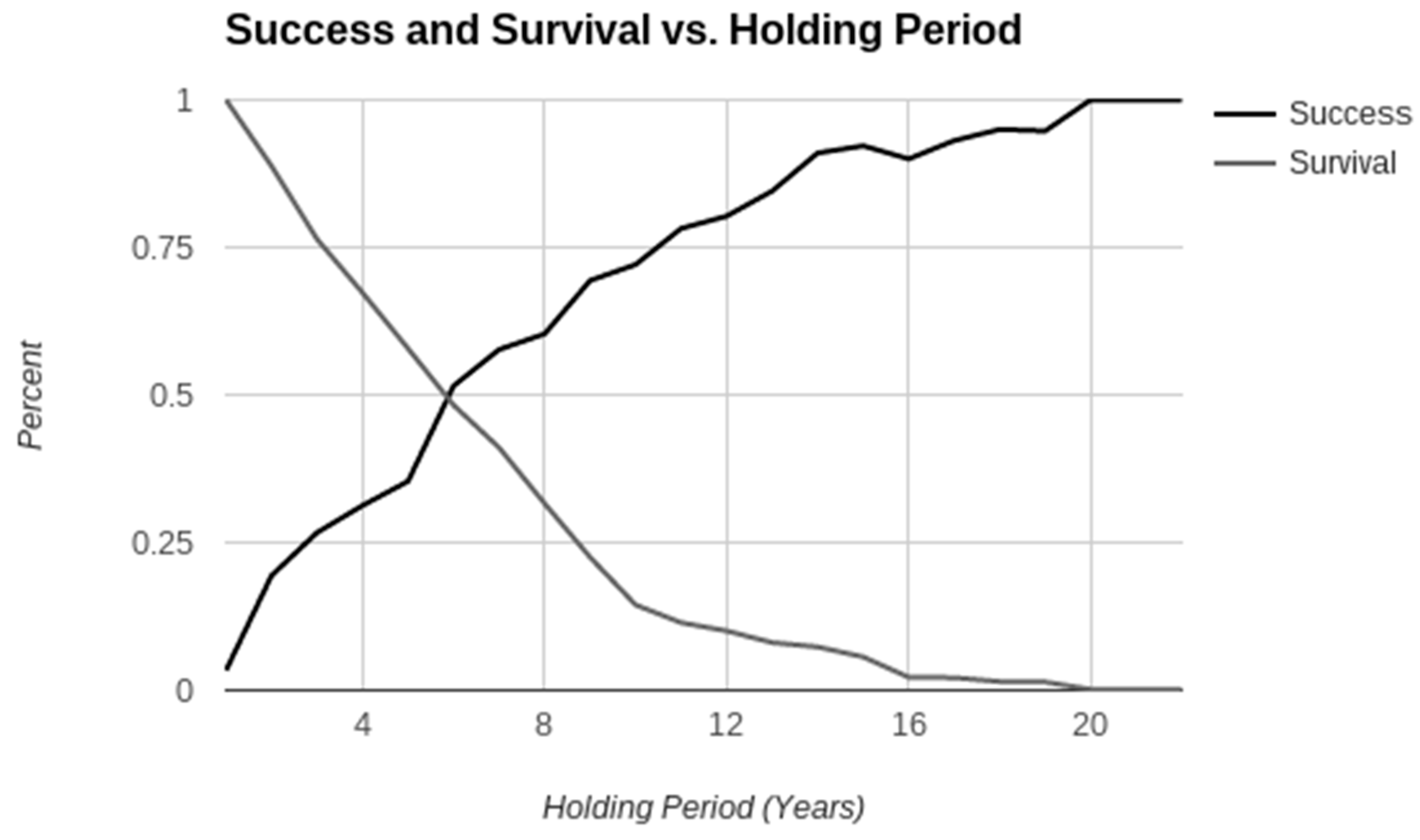
The ETF that survives tends to be the more successful choice. This can be clearly depicted in the Figure 1 below:
Only 50% of the ETFs examined survived beyond 6 years, and the success rate at that point was 50% as well. The average investor would like to have her retirement in a routinely successful fund. The chances of identifying that particular set of ETFs looks difficult; throwing a dart, as was once suggested as a reasonable course of action, does not appear to be a reliable method today (Malkiel 1998).
To be fair, the original buy and hold strategy was meant to be carried out using index fund vehicles. Investors were encouraged to invest in a broadly diversified index that would mirror the stock market. To see if there was any difference in our results if we focused on this aspect of the strategy, we first consider ETF success by asset class in Table 4 and then by sector in Table 5 below. By asset class the results are summarized:
Broadly speaking, the Equity categorization fits most closely with the buy and hold recommendation, although there are probably some ETFs in there that are not diversified index funds. For a one-year holding period, 66.67% of the equity ETFs outcomes were positive ones, which is a little higher than was true for the sample overall. If you look at a 10 year holding period, approximately both the equity and the total sample saw 95% positive outcomes.
Also, here is the probability of no loss by asset class.
The following results were not included in the table due to low numbers of ETF’s (commodities (1)).
In Table 5 above, the picture of success for equity ETFs looks tougher to achieve when isolated from the entire sample. Only 0.55% of equity ETFs were able to earn a positive return over a rolling one-year holding period, as contrasted with 3.77% for the wider sample. By year 10, it looks like equity ETF success has risen a bit faster than the sample overall, but still lags behind a bit, at 69.06% compared to 72.08%.
When the ETFs are sorted by sector, see Table 6 below, we can see that the large-cap, the mid-cap, the multi-cap, and even the small-cap sectors tend to do a bit better for each holding period length than the ETF sector average overall:
The ETFs that are focused on market capitalization all do much better in terms of the chances of returning a positive return than ETFs do overall. When we set the holding period at one year, each of the four market capitalization type funds—large-cap, mid-cap, multi-cap, and small-cap—have positive return outcomes between 67%–78%. Each of these is above 95% when holding periods roll every 10 years. This is a bit higher than the outcome for ETFs overall. Intuitively, this makes sense in that there is typically less volatility in these broad capitalization sectors than the more specialized sectors like power, natural resources, or Europe. We would expect it to take fewer holding periods to reach a high probability of no reduction of principal. However, this result may be misleading as we are not benchmarking to what might be an “acceptable return” for an investor.
The probability of no loss by sector is shown in Table 7:
ETFs left out of the table, but included in the average calculation: (Alternative investments (2), Commodities (1), Construction (2), Consumer-non-cyclical (2), Consumer services (1), Consumer staples (1), Defense (1), Environmental (1), Healthcare (2), Managed eETF (1), Mixed asset (4), Precious metals (1), Taxable bonds (3), Transportation (2)
Notably, none of the sectors included funds that had 100% success for every one-year holding period. What emerges from the table above is just how unsuccessful investing in ETFs that specialize could be. With a five-year rolling average, none of the ETFs in these sectors could boast no losses! The investor is hard pressed to find a good ETF there without some patience, at least for the historical time period examined here.
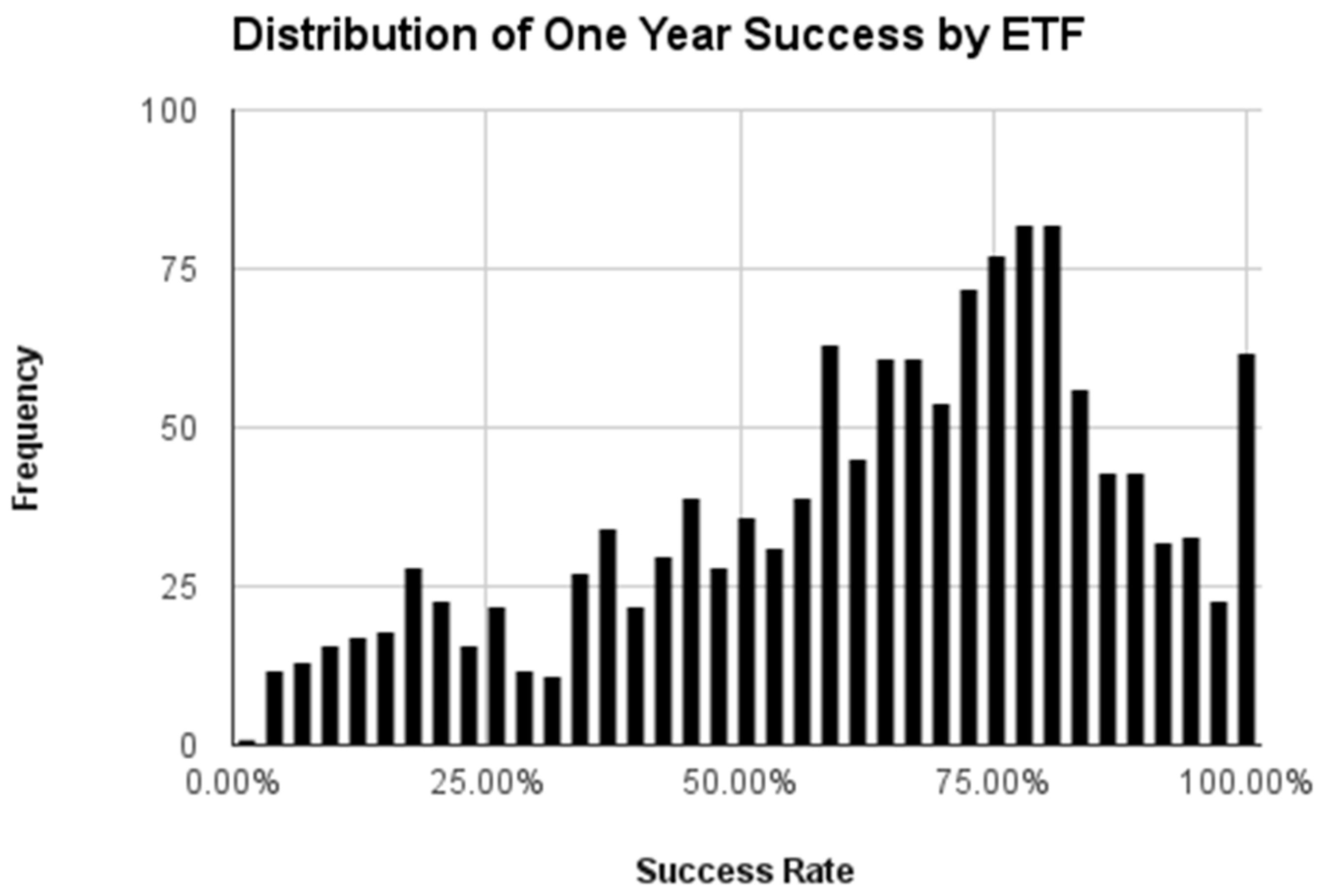
One other perspective from which to look at our results is to compare frequency distributions across holding periods. Below are the frequency distributions for positive return outcomes for the one-year and the three-year rolling holding periods.
What is striking when comparing the two distributions in Figure 2 and Figure 3 below is how bimodal the distribution becomes just by moving from a one-year rolling holding period to a three-year. Nearly 24 percent of ETFs with a three-year holding period window produced a loss of principal or didn’t survive in the market place long enough for a three-year holding period.
Finally, to see if there is anything unique about ETFs, we have calculated the probabilities for all companies listed on the NYSE as a means of comparison in Table 8 below:
While this data does look similar to the results for ETFs overall, comparing the difference of the mean between the two populations in proportion shows that the two populations are statistically different from one another in nineteen out of the twenty-three years at a 95% confidence level. The ETF probability of positive return is a little lower for a one-year holding period, but 10% higher at the 10-year holding period. However, we do see similar behavior in the rates of success within the compound return calculations. While we won’t explicitly do it here, more research needs to be done to look at broader patterns of holding periods and compound returns.
5. Conclusions
We were surprised to discover so much variability in compound returns for the NASDAQ ETFs. Given our results, we found that it is relatively unlikely for one to gain a positive compound return on the NASDAQ ETFs with a buy and hold strategy. We say this because for most of the ETFs, it takes roughly ten years before the probability of a positive gain clears 95%, much less some specified required return hurdle. Notice we are not saying that if you held long enough you would not be able to generate a gain, just that it is less likely that many folks would do so in this more volatile stock market. Additionally, our calculations occur before transaction costs.
Given the volatility of the stock market, it becomes less likely that the average investor would be willing to hold for the length of time necessary, riding through the downs of the market. This suggests that perhaps buy and hold is not a strategy that is as effective as it was once thought to be. Ask yourself: Would you be willing to continue to hold an investment if you saw the market value below your principal after five years? For investors and even for finance professionals providing the advice, the importance of this result is that a no to this question impacts retirement planning. How many clients of advisors or individuals can stay the course when they see anemic, or, in our case of ETFs, no gain on principal? Behaviorally for investors, this could be magnified because many individuals saving for retirement may have expectations that rely on old rules of thumb for returns and/or have not started saving for retirement until later in life. This finding is relevant because it may tell us we need to dramatically change the way we view the common wisdom of passive investing.
Further, exacerbating the lower likelihood of success with buy and hold is the small percentage of ETFs that actually survive through the holding period requirements. Investors must be wise about the ETFs they choose. It does look like ETFs categorized by market capitalization do pronouncedly better than ETFs overall. When you look back at the original buy and hold recommendations, investment under buy and hold was directed towards a broadly diversified market index fund. A positive return does appear to be more likely among this diversified categorization, which might ultimately support the idea of buy and hold.
While certainly not conclusive, more research in this area is warranted, as it appears long run average returns may not be a good indicator of future performance and are at best in the current environment a relatively high upper bound on portfolio performance. Our focus is on the buy and hold strategy which we have applied to ownership in ETFs, but advocates to the approach originally intended investors to use mutual funds. Because the two products are not exactly the same, using our algorithm to look at the returns for mutual funds before and after the marked increase in market volatility is the natural next step. Beyond the application of our study methods to other investment products, consideration of buy and hold versus other strategies or simple trading rules would highlight whether buy and hold is really a strategy for a bygone era in stock market investing. Ultimately, these instances are really more about bigger considerations involving how academics measure risk versus how investors experience it. If risk is best captured by price volatility, then a world with a lot more volatility may mean that the old advice and the old strategies to wait and see do not serve investors as well. If the market has fundamentally changed, so must the advice for getting that nest egg to retirement.
Author Contributions
Methodology, R.S.; Data Curation, R.S.; Writing-Original Draft Preparation, N.L.L.-S.; Writing-Review & Editing, N.L.L.-S.
Conflicts of Interest
The authors declare no conflict of interest.
References
- Angel, James J., Todd J. Broms, and Gary L. Gastineau. 2016. ETF Transaction Costs Are Often Higher than Investors Realize. The Journal of Portfolio Management 42: 65–75. [Google Scholar] [CrossRef]
- Antoniewicz, Rochelle, and Jane Heinrichs. 2014. Understanding exchange-traded funds: How ETFs work. ICI Research Perspective. [Google Scholar] [CrossRef]
- Blume, Marshall E. 1974. Unbiased estimators of long-run expected rates of return. Journal of the American Statistical Association 69: 634–38. [Google Scholar] [CrossRef]
- Buetow, Gerald W., and Brian J. Henderson. 2012. An empirical analysis of exchange-traded funds. Journal of Portfolio Management 38: 112–27. [Google Scholar] [CrossRef]
- Chen, Haiwei, Sang Heon Shin, and Xu Sun. 2015. Return-enhancing strategies with international ETFs: Exploiting the turn-of-the-month effect. Financial Services Review 24: 271–88. [Google Scholar]
- Coen, Andrew, and Paula Vasan. 2014. ETF 1Q Report: New Products, Fees. Money Management Executive 22: 1–6. [Google Scholar]
- De Jong, Jack C., Jr., and S. Ghon Rhee. 2008. Abnormal returns with momentum/contrarian strategies using exchange-traded funds. Journal of Asset Management 9: 289–299. [Google Scholar] [CrossRef]
- Dellva, Wilfred L. 2001. Exchange-Traded Funds Not for Everyone. Journal of Financial Planning 14: 110–24. [Google Scholar]
- Fama, Eugene. 1970. Efficient Capital Markets: A Review of Theory and Empirical Work. Journal of Finance 25: 383–417. [Google Scholar] [CrossRef]
- Gastineau, Gary L. 2004. The Benchmark Index ETF Performance Problem. Journal of Portfolio Management 30: 96–103. [Google Scholar] [CrossRef]
- Krouse, Sarah. 2015. Vanguard Group Took in $196 Billion of Investor Cash through October; Inflows Put Mutual-Fund Firm on Pace to Top 2014 Record. Wall Street Journal. November 16. Available online: https://www.wsj.com/articles/vanguard-group-took-in-196-billion-of-investor-cash-through-october-1447440046 (accessed on 10 November 2016).
- Lim, Kian-Ping, and Robert Brooks. 2011. The evolution of stock market efficiency over time: A survey of the empirical literature. Journal of Economic Surveys 25: 69–108. [Google Scholar] [CrossRef]
- Lo, Andrew W. 2004. The adaptive markets hypothesis: Market efficiency from an evolutionary perspective. Journal of Portfolio Management. Forthcoming. Available online: https://ssrn.com/abstract=602222 (accessed on 23 July 2016).
- Lo, Andrew W. 2005. Reconciling efficient markets with behavioral finance: The adaptive markets hypothesis. Journal of Investment Consulting 7: 21–44. [Google Scholar]
- Lo, Andrew W. 2012. Adaptive Markets and the New World Order (corrected May 2012). Financial Analysts Journal 68: 18–29. [Google Scholar] [CrossRef] [Green Version]
- Lo, Andrew W., and A. Craig MacKinlay. 1999. A Non-Random Walk Down Wall Street. Princeton: Princeton University Press. [Google Scholar]
- Maiello, Michael, and Megan Johnston. 2006. ETF-O-Mania. Forbes 178: 142–46. Available online: https://www.forbes.com/home/free_forbes/2006/0918/142.html (accessed on 1 August 2016).
- Malkiel, Burton G. 1998. A Random Walk Down Wall Street: The Best Investment Advice for the New Century. New York: W.W. Norton & Company. [Google Scholar]
- Malkiel, Burton G. 2003. The efficient market hypothesis and its critics. The Journal of Economic Perspectives 17: 59–82. [Google Scholar] [CrossRef]
- Ross, Stephen A., Randolph Westerfield, and Bradford D. Jordan. 2015. Fundamentals of Corporate Finance, 11th ed. New York: McGraw-Hill Education, p. 390. [Google Scholar]
- Samuelson, Paul A. 1965. Proof that properly anticipated prices fluctuate randomly. Industrial Management Review 6: 41–90. [Google Scholar]
- Toolson, Richard B. 2012. When to Consider Tax Efficient ETFs in Taxable Accounts as an Alternative to High-Fee 401(k) Plans. Journal of Taxation of Investments 29: 3–18. [Google Scholar]
- Wile, Rob. 2012. ANDREW LO: Buy-And-Hold Doesn’t Work Anymore. Business Insider. February 27. Available online: http://www.businessinsider.com/andrew-lo-buy-and-hold-doesnt-work-anymore-2012-2 (accessed on 15 August 2016).
Figure 1.
Success and Holding Period.

Figure 2.
Distribution of One Year Success.

Figure 3.
Distribution of Three Year Success.


Table 1.
BLDRS Developed Markets 100 ADR Index Fund (ADRD) Positive Gain to Principal Percentages.
| Holding Period (Years) | Probability of Gain |
|---|---|
| 1 | 68.46% |
| 2 | 74.45% |
| 3 | 70.40% |
| 4 | 63.72% |
| 5 | 67.33% |
| 6 | 71.91% |
| 7 | 94.81% |
| 8 | 86.15% |
| 9 | 94.34% |
| 10 | 100.00% |
| 11 | 100.00% |
| 12 | 100.00% |
| 13 | 100.00% |
Table 2.
Success Rates for All NASDAQ Exchange Traded Funds (ETF’s).
| Holding Period (Years) | Mean Prob. of a Gain | Min | Max | Range | Std Dev | Skew | CV | Number of ETF’s | Survival Rate |
|---|---|---|---|---|---|---|---|---|---|
| 1 | 59.49% | 1.30% | 100.00% | 98.70% | 24.03% | −0.5792 | 0.404 | 1374 | |
| 2 | 67.12% | 1.16% | 100.00% | 98.84% | 27.43% | −0.6458 | 0.409 | 1228 | 89.37% |
| 3 | 72.71% | 1.22% | 100.00% | 98.78% | 26.86% | −0.8895 | 0.369 | 1055 | 76.78% |
| 4 | 75.18% | 1.18% | 100.00% | 98.82% | 26.85% | −0.9540 | 0.357 | 944 | 68.70% |
| 5 | 78.29% | 2.74% | 100.00% | 97.26% | 25.83% | −1.1139 | 0.330 | 799 | 58.15% |
| 6 | 83.73% | 4.55% | 100.00% | 95.46% | 24.76% | −1.5002 | 0.296 | 673 | 48.98% |
| 7 | 87.11% | 6.67% | 100.00% | 93.33% | 22.88% | −1.8630 | 0.263 | 571 | 41.56% |
| 8 | 87.24% | 3.19% | 100.00% | 96.81% | 23.60% | −2.0863 | 0.271 | 452 | 32.90% |
| 9 | 93.20% | 9.00% | 100.00% | 91.00% | 16.12% | −3.0983 | 0.173 | 332 | 24.16% |
| 10 | 95.97% | 10.00% | 100.00% | 90.00% | 11.97% | −5.0068 | 0.125 | 207 | 15.07% |
| 11 | 97.02% | 40.79% | 100.00% | 59.21% | 8.81% | −4.0153 | 0.091 | 166 | 12.08% |
| 12 | 96.90% | 43.75% | 100.00% | 56.25% | 8.80% | −3.7230 | 0.091 | 138 | 10.04% |
| 13 | 97.71% | 55.77% | 100.00% | 44.23% | 7.71% | −4.0150 | 0.079 | 112 | 8.15% |
| 14 | 98.01% | 50.00% | 100.00% | 50.00% | 7.59% | −4.4286 | 0.077 | 101 | 7.35% |
| 15 | 97.38% | 36.36% | 100.00% | 63.64% | 10.29% | −4.2739 | 0.106 | 82 | 5.97% |
| 16 | 97.98% | 66.67% | 100.00% | 33.33% | 7.28% | −3.8001 | 0.074 | 32 | 2.33% |
| 17 | 99.17% | 83.33% | 100.00% | 16.67% | 3.35% | −4.2810 | 0.034 | 30 | 2.18% |
| 18 | 98.96% | 79.17% | 100.00% | 20.83% | 4.66% | −4.4721 | 0.047 | 20 | 1.46% |
| 19 | 99.12% | 83.33% | 100.00% | 16.67% | 3.82% | −4.3589 | 0.039 | 19 | 1.38% |
| 20 | 100.00% | 100.00% | 100.00% | 2 | 0.15% | ||||
| 21 | 100.00% | 100.00% | 100.00% | 1 | 0.07% | ||||
| 22 | 100.00% | 100.00% | 100.00% | 1 | 0.07% | ||||
| 23 | 100.00% | 100.00% | 100.00% | 1 | 0.07% |
Table 3.
Percent of NASDAQ ETF’s that had a 100 Percent Success Rate by Holding Period.
| Holding Period (Years) | Success |
|---|---|
| 1 | 3.37% |
| 2 | 19.41% |
| 3 | 26.68% |
| 4 | 31.26% |
| 5 | 35.36% |
| 6 | 51.52% |
| 7 | 57.68% |
| 8 | 60.32% |
| 9 | 69.38% |
| 10 | 72.08% |
| 11 | 78.21% |
| 12 | 80.29% |
| 13 | 84.55% |
| 14 | 91.00% |
| 15 | 92.21% |
| 16 | 90.00% |
| 17 | 93.10% |
| 18 | 95.00% |
| 19 | 94.74% |
| 20 | 100.00% |
| 21 | 100.00% |
| 22 | 100.00% |
Table 4.
NASDAQ ETF Positive Return Probabilities by Asset Class.
| Holding Period (Years) | Bonds | Equity | Fixed Income | Multi-Asset |
|---|---|---|---|---|
| 1 | 82.78% | 66.76% | 77.01% | 66.28% |
| 2 | 96.64% | 70.66% | 86.98% | 82.57% |
| 3 | 99.55% | 74.54% | 90.58% | 88.53% |
| 4 | 100.00% | 75.56% | 94.63% | 92.47% |
| 5 | 100.00% | 80.85% | 97.72% | 93.13% |
| 6 | 100.00% | 85.70% | 98.75% | 94.48% |
| 7 | 87.79% | 100.00% | 100.00% | |
| 8 | 86.39% | 100.00% | 100.00% | |
| 9 | 93.10% | 100.00% | 100.00% | |
| 10 | 95.52% | 100.00% | 100.00% | |
| 11 | 96.49% | 100.00% | ||
| 12 | 96.54% | 100.00% | ||
| 13 | 97.53% | 100.00% | ||
| 14 | 97.93% | |||
| 15 | 97.13% | |||
| 16 | 98.24% | |||
| 17 | 99.21% | |||
| 18 | 98.91% | |||
| 19 | 99.04% | |||
| 20 | 100.00% | |||
| 21 | 100.00% | |||
| 22 | 100.00% | |||
| 23 | 100.00% |
Table 5.
NASDAQ Probability of No Loss by Asset Class.
| Holding Period (Years) | Bonds | Equity | Fixed Income | Multi-Asset |
|---|---|---|---|---|
| 1 | 16.67% | 0.55% | 3.45% | 6.00% |
| 2 | 58.33% | 8.92% | 39.66% | 43.00% |
| 3 | 91.67% | 16.70% | 62.07% | 61.82% |
| 4 | 100.00% | 19.48% | 76.36% | 77.78% |
| 5 | 100.00% | 26.34% | 93.75% | 75.00% |
| 6 | 100.00% | 45.63% | 97.50% | 78.57% |
| 7 | 50.26% | 100.00% | 100.00% | |
| 8 | 50.93% | 100.00% | 100.00% | |
| 9 | 65.22% | 100.00% | 100.00% | |
| 10 | 69.06% | 100.00% | 100.00% | |
| 11 | 75.89% | 100.00% | ||
| 12 | 78.23% | 100.00% | ||
| 13 | 83.96% | 100.00% | ||
| 14 | 91.00% | |||
| 15 | 92.50% | |||
| 16 | 90.63% | |||
| 17 | 93.10% | |||
| 18 | 95.00% | |||
| 19 | 94.74% | |||
| 20 | 100.00% | |||
| 21 | 100.00% | |||
| 22 | 100.00% | |||
| 23 | 100.00% |
Table 6.
NASDAQ ETF Success by Sector (In Percent).
| Holding Period (Years) | Average | Large Cap | Mid-Cap | Multi-Cap | Small Cap |
|---|---|---|---|---|---|
| 1 | 67.94 | 78.2 | 72.8 | 67.7 | 67.5 |
| 2 | 71.42 | 80.7 | 76.0 | 74.6 | 71.7 |
| 3 | 74.42 | 80.8 | 77.4 | 74.8 | 74.1 |
| 4 | 75.59 | 81.3 | 80.6 | 83.2 | 76.0 |
| 5 | 80.15 | 89.3 | 92.1 | 91.0 | 87.5 |
| 6 | 84.06 | 97.1 | 97.1 | 93.7 | 96.0 |
| 7 | 85.51 | 96.6 | 96.8 | 97.3 | 97.4 |
| 8 | 83.62 | 94.6 | 98.1 | 97.5 | 97.6 |
| 9 | 92.88 | 95.6 | 97.8 | 99.5 | 98.5 |
| 10 | 95.49 | 96.1 | 100.0 | 100.0 | 97.9 |
| 11 | 96.34 | 96.7 | 100.0 | 100.0 | 99.9 |
| 12 | 96.28 | 97.4 | 100.0 | 100.0 | 100.0 |
| 13 | 97.26 | 98.2 | 100.0 | 100.0 | 100.0 |
| 14 | 97.46 | 99.5 | 100.0 | 100.0 | 100.0 |
| 15 | 92.74 | 100.0 | 100.0 | 100.0 | 100.0 |
| 16 | 97.20 | 100.0 | 100.0 | ||
| 17 | 99.51 | 100.0 | 100.0 | ||
| 18 | 98.58 | 100.0 | 100.0 | ||
| 19 | 98.75 | 100.0 | 100.0 | ||
| 20 | 100.0 | 100.0 | |||
| 21 | 100.0 | ||||
| 22 | 100.0 | ||||
| 23 | 100.0 |
Table 7.
NASDAQ Probability of No Loss by Sector (In Percent).
| Holding Period (Years) | Average | Large Cap | Mid-Cap | Multi-Cap | Small Cap |
|---|---|---|---|---|---|
| 1 | 0.00 | 0.00 | 0.00 | 0.00 | 0.00 |
| 2 | 8.26 | 19.64 | 0.00 | 10.00 | 0.00 |
| 3 | 13.75 | 23.21 | 3.33 | 10.00 | 12.90 |
| 4 | 18.32 | 23.64 | 13.33 | 33.33 | 12.90 |
| 5 | 29.19 | 32.73 | 37.93 | 33.33 | 27.59 |
| 6 | 47.22 | 61.82 | 86.21 | 77.78 | 78.57 |
| 7 | 54.15 | 59.52 | 67.86 | 60.00 | 64.00 |
| 8 | 49.27 | 60.98 | 82.14 | 60.00 | 83.33 |
| 9 | 64.51 | 65.79 | 92.31 | 80.00 | 86.96 |
| 10 | 70.47 | 58.62 | 100.00 | 100.00 | 87.50 |
| 11 | 83.01 | 58.33 | 100.00 | 100.00 | 92.31 |
| 12 | 81.71 | 80.00 | 100.00 | 100.00 | 100.00 |
| 13 | 85.84 | 87.50 | 100.00 | 100.00 | 100.00 |
| 14 | 90.22 | 93.75 | 100.00 | 100.00 | 100.00 |
| 15 | 85.65 | 100.00 | 100.00 | 100.00 | 100.00 |
| 16 | 85.83 | 100.00 | 100.00 | ||
| 17 | 95.83 | 100.00 | 100.00 | ||
| 18 | 93.75 | 100.00 | 100.00 | ||
| 19 | 93.75 | 100.00 | 100.00 | ||
| 20 | 100.00 | 100.00 | |||
| 21 | 100.00 | ||||
| 22 | 100.00 | ||||
| 23 | 100.00 |
Table 8.
NYSE Company Probabilities.
| Holding Period (Years) | Mean Prob. of a Positive Gain | Min | Max | Range | Std Dev | Skew | CV | Number of Firms | Survival Rate |
|---|---|---|---|---|---|---|---|---|---|
| 1 | 63.93% | 11.11% | 100.00% | 88.89% | 16.42% | −0.8018 | 0.2569 | 2494 | |
| 2 | 70.48% | 11.76% | 100.00% | 88.24% | 18.44% | −0.7688 | 0.2616 | 2344 | 93.99% |
| 3 | 74.34% | 11.54% | 100.00% | 88.46% | 19.29% | −0.9080 | 0.2595 | 2218 | 88.93% |
| 4 | 76.04% | 5.56% | 100.00% | 94.44% | 20.40% | −1.0236 | 0.2683 | 2074 | 83.16% |
| 5 | 78.04% | 6.67% | 100.00% | 93.33% | 20.84% | −1.1022 | 0.2671 | 1972 | 79.07% |
| 6 | 80.57% | 9.09% | 100.00% | 90.91% | 22.03% | −1.2595 | 0.2734 | 1881 | 75.42% |
| 7 | 82.11% | 1.92% | 100.00% | 98.08% | 22.42% | −1.4006 | 0.2731 | 1809 | 72.53% |
| 8 | 83.38% | 0.71% | 100.00% | 99.29% | 22.73% | −1.5548 | 0.2726 | 1750 | 70.17% |
| 9 | 85.27% | 4.14% | 100.00% | 95.86% | 21.91% | −1.7315 | 0.2569 | 1668 | 66.88% |
| 10 | 86.99% | 4.29% | 100.00% | 95.71% | 21.06% | −1.8993 | 0.2421 | 1601 | 64.19% |
| 11 | 87.91% | 4.48% | 100.00% | 95.52% | 20.88% | −2.0529 | 0.2375 | 1536 | 61.59% |
| 12 | 88.98% | 3.67% | 100.00% | 96.33% | 20.38% | −2.1830 | 0.2290 | 1458 | 58.46% |
| 13 | 89.77% | 3.33% | 100.00% | 96.67% | 20.51% | −2.3112 | 0.2284 | 1377 | 55.21% |
| 14 | 90.27% | 5.74% | 100.00% | 94.26% | 20.39% | −2.3773 | 0.2259 | 1314 | 52.69% |
| 15 | 90.80% | 9.68% | 100.00% | 90.32% | 20.13% | −2.4882 | 0.2217 | 1254 | 50.28% |
| 16 | 91.32% | 9.14% | 100.00% | 90.86% | 20.48% | −2.6440 | 0.2243 | 1213 | 48.64% |
| 17 | 92.17% | 3.45% | 100.00% | 96.55% | 20.05% | −2.9179 | 0.2175 | 1172 | 46.99% |
| 18 | 93.15% | 8.33% | 100.00% | 91.67% | 18.43% | −3.2055 | 0.1979 | 1114 | 44.67% |
| 19 | 94.32% | 4.67% | 100.00% | 95.33% | 16.73% | −3.5911 | 0.1774 | 1052 | 42.18% |
| 20 | 95.40% | 16.67% | 100.00% | 83.33% | 14.59% | −3.8814 | 0.1529 | 1000 | 40.10% |
| 21 | 95.70% | 6.06% | 100.00% | 93.94% | 15.00% | −4.2055 | 0.1568 | 946 | 37.93% |
| 22 | 95.74% | 12.50% | 100.00% | 87.50% | 15.41% | −4.3247 | 0.1609 | 856 | 34.32% |
| 23 | 96.65% | 6.67% | 100.00% | 93.33% | 13.33% | −5.0259 | 0.1379 | 793 | 31.80% |
| 24 | 97.01% | 36.36% | 100.00% | 63.64% | 12.87% | −5.3289 | 0.1327 | 732 | 29.35% |
| 25 | 97.68% | 13.33% | 100.00% | 86.67% | 10.80% | −6.0647 | 0.1105 | 636 | 25.50% |
| 26 | 97.58% | 5.56% | 100.00% | 94.44% | 11.59% | −5.9400 | 0.1188 | 615 | 24.66% |
| 27 | 97.82% | 90.09% | 100.00% | 9.91% | 11.04% | −6.3948 | 0.1129 | 501 | 20.09% |
| 28 | 98.45% | 20.00% | 100.00% | 80.00% | 9.10% | −7.5345 | 0.0924 | 478 | 19.17% |
| 29 | 97.73% | 36.36% | 100.00% | 63.64% | 11.64% | −6.3918 | 0.1191 | 318 | 12.75% |
| 30 | 98.69% | 23.81% | 100.00% | 76.19% | 8.01% | −8.3285 | 0.0812 | 285 | 11.43% |
| 31 | 98.31% | 20.51% | 100.00% | 79.49% | 10.33% | −7.8625 | 0.1051 | 245 | 9.82% |
| 32 | 97.61% | 14.58% | 100.00% | 85.42% | 12.98% | −6.2444 | 0.1330 | 178 | 7.14% |
| 33 | 98.65% | 94.59% | 100.00% | 5.41% | 9.63% | −8.4064 | 0.0976 | 161 | 6.46% |
| 34 | 99.06% | 71.56% | 100.00% | 28.44% | 6.63% | −8.3752 | 0.0669 | 136 | 5.45% |
| 35 | 99.08% | 75.00% | 100.00% | 25.00% | 4.57% | −5.5193 | 0.0462 | 106 | 4.25% |
| 36 | 99.59% | 92.94% | 100.00% | 7.06% | 3.25% | −9.3498 | 0.0326 | 100 | 4.01% |
| 37 | 99.54% | 65.75% | 100.00% | 34.25% | 3.73% | −8.9559 | 0.0375 | 86 | 3.45% |
| 38 | 99.61% | 68.85% | 100.00% | 31.15% | 3.38% | −9.1817 | 0.0339 | 85 | 3.41% |
| 39 | 99.63% | 97.96% | 100.00% | 2.04% | 3.16% | −8.9880 | 0.0317 | 82 | 3.29% |
| 40 | 99.51% | 64.86% | 100.00% | 35.14% | 4.17% | −8.4261 | 0.0419 | 71 | 2.85% |
| 41 | 99.49% | 64.00% | 100.00% | 36.00% | 4.30% | −8.3666 | 0.0433 | 70 | 2.81% |
| 42 | 99.44% | 61.54% | 100.00% | 38.46% | 4.63% | −8.3066 | 0.0466 | 69 | 2.77% |
| 43 | 100.00% | 100.00% | 100.00% | 68 | 2.73% | ||||
| 44 | 100.00% | 100.00% | 100.00% | 26 | 1.04% | ||||
| 45 | 100.00% | 100.00% | 100.00% | 26 | 1.04% | ||||
| 46 | 100.00% | 100.00% | 100.00% | 26 | 1.04% | ||||
| 47 | 100.00% | 100.00% | 100.00% | 9 | 0.36% | ||||
| 48 | 100.00% | 100.00% | 100.00% | 9 | 0.36% | ||||
| 49 | 100.00% | 100.00% | 100.00% | 9 | 0.36% | ||||
| 50 | 100.00% | 100.00% | 100.00% | 9 | 0.36% | ||||
| 51 | 100.00% | 100.00% | 100.00% | 9 | 0.36% | ||||
| 52 | 100.00% | 100.00% | 100.00% | 9 | 0.36% | ||||
| 53 | 100.00% | 100.00% | 100.00% | 9 | 0.36% | ||||
| 54 | 100.00% | 100.00% | 100.00% | 9 | 0.36% |
© 2018 by the authors. Licensee MDPI, Basel, Switzerland. This article is an open access article distributed under the terms and conditions of the Creative Commons Attribution (CC BY) license (http://creativecommons.org/licenses/by/4.0/).
Share and Cite
MDPI and ACS Style
Sanderson, R.; Lumpkin-Sowers, N.L. Buy and Hold in the New Age of Stock Market Volatility: A Story about ETFs. Int. J. Financial Stud. 2018, 6, 79. https://doi.org/10.3390/ijfs6030079
AMA Style
Sanderson R, Lumpkin-Sowers NL. Buy and Hold in the New Age of Stock Market Volatility: A Story about ETFs. International Journal of Financial Studies. 2018; 6(3):79. https://doi.org/10.3390/ijfs6030079
Chicago/Turabian StyleSanderson, Rohnn, and Nancy L. Lumpkin-Sowers. 2018. "Buy and Hold in the New Age of Stock Market Volatility: A Story about ETFs" International Journal of Financial Studies 6, no. 3: 79. https://doi.org/10.3390/ijfs6030079
Note that from the first issue of 2016, this journal uses article numbers instead of page numbers. See further details here.