Technical Efficiency of Banks in Central and Eastern Europe


1
Faculty of National Economy, University of Economics in Bratislava, 852 35 Bratislava, Slovakia
2
Faculty of Business Administration, Masaryk University Brno, 601 77 Brno, Czech Republic
Int. J. Financial Stud. 2018, 6(3), 66; https://doi.org/10.3390/ijfs6030066
Submission received: 8 May 2018
/
Revised: 2 July 2018
/
Accepted: 3 July 2018
/
Published: 17 July 2018
Abstract
:The purpose of this article is to examine what affected the technical efficiency of banks in Central and Eastern European countries during the financial crisis. Firstly, this article analyzes the technical efficiency of banks in the selected countries in Central and Eastern Europe during the period 2006–2013. In this article, the technical efficiency of Central and Eastern European banks is explored in respect to the size of the banks (large or small) and their belonging in a specific group of countries. The results of the analysis show a strong association between the numbers of efficient banks and belonging of banks in the group of V4 countries (Visegrad countries are the Czech Republic, Hungary, Poland, and Slovakia). The banks in Balkan countries have a negative association with the number of efficient banks in the group; the banks in this group of countries have the highest average efficiency (when the output was net interest margin). There is a weak association between the number of efficient banks and their belonging in the group of Baltic countries. The bank efficiency and the size of the bank’s assets are also weakly associated. Secondly, the results of panel regression models for the specific groups of countries (V4, Baltic, and Balkan countries), as well as for the whole group of Central and Eastern European countries show that the customer deposits had a positive impact on the technical efficiency of banks during the financial crisis.
JEL Classification:
G21; C58; C141. Introduction
The banking sectors in Central and Eastern European countries have undergone a complex process of restructuring and subsequent privatization. This intensive reform process used similar instruments and similar speed of reform adoptions, but the impact of these changes among Central and Eastern European (CEE) countries is different. Understanding the drivers of bank efficiency is an important part of bank management and regulation.
The purpose of this article is to examine what affected the technical efficiency of Eastern European banks during the financial crisis. This article analyzes the technical efficiency of banks in the selected countries in Central and Eastern Europe (Czech Republic, Croatia, Hungary, Estonia, Latvia, Lithuania, Poland, Romania, Slovakia, and Slovenia) during the period 2006–2013. In the article, the technical efficiency of Central and Eastern European banks is explored in respect to the size of the banks (large or small) and their belonging in a specific group of countries.
Previous research shows that the regulatory changes and EU standards have a positive impact on the efficiency of banks in CEE countries (Nurboja and Košak 2017; Košak and Zajc 2006).
A considerable part of the research is devoted to the relationship between the efficiency of banks and their ownership. Many studies conclude that the privatization of state-owned banks increased the efficiency of banks in CEE countries (Hasan and Marton 2003; Matousek and Taci 2004). Doan et al. (2018) evaluated the bank efficiency by combining two interrelated dimensions: bank income diversification and ownership of banks.
Research within CEE also differs in scope of research—for which countries the research is performed. There are studies dealing with groups of countries in CEE, as well as country–specific studies. Efficiency of banks in the V4 countries (Czech Republic, Hungary, Poland, and Slovakia) has been analyzed for several time periods and with results respecting real economic development (Stavárek 2005; Svitalkova 2014; Palečková 2015).
Pancurova and Lyocsa (2013) included 11 countries in the analysis: Bulgaria, Croatia, Czech Republic, Hungary, Estonia, Lituania, Latvia, Poland, Romania, Slovakia, and Slovenia in the period 2005–2008. Košak and Zajc (2006) analyzed the new EU member countries (Czech Republic, Hungary, Poland, Slovakia, and Slovenia) during the period 1996–2003. Degl’Innocenti et al. (2017) analyzed 9 CEE countries (Bulgaria, Croatia, Czech Republic, Estonia, Hungary, Latvia, Lithuania, Poland, and Romania) using a window-based weight assurance region approach over the period 2004–2015.
Molnar and Holló (2011) evaluated the efficiency of banks in Hungary in comparison with the EU banks during the period 2004–2008. They compared their cost efficiency using the Stochastic Frontier Approach (SFA).
Gallizo et al. (2017) analyzed the efficiency of banks in Baltic countries (Estonia, Latvia, Lithuania) during the period 2000–2013 using the Bayesian stochastic frontier models. Novickytė and Droždz (2018) evaluated bank performance in a low interest rate environment of the banks owned by the Nordic parent group.
There are several publications focused on individual CEE countries. Zimková (2014) analyzed the bank efficiency in Slovakia, Řepková (2014) in the Czech Republic, Hasan and Marton (2003) in Hungary, Woznievska (2008) in Poland.
The existing studies are inspirational for a new insight into the efficiency of banks. In particular, there is a lack of studies looking at certain differences that are present in the group of countries in CEE, which are geographically or economically closer to each other. The Data Envelope Analysis (DEA) analysis compares the relative efficiency of banks. Changing the structure of the analyzed banks provides different results of efficiency. Therefore, the results of differently structured groups of countries lead to interesting conclusions. The research is motivated by the importance of the banking sector in Central and Eastern Europe; however, the importance of this banking sector is much broader, not only regional. The paper is important in two respects: (1) It investigates what affected the technical efficiency of Eastern European banks during the financial crisis in respect to the size of banks (large or small) and their belonging in a specific group of countries; and (2) considering that the largest banks of Central and Eastern Europe are parts of Western European banks (Raiffeisen, Erste Bank, Intesa Sanpaolo, UniCredit), the stability of Central and Eastern European banks may also affect the banks in Western Europe. Therefore, the banking system of Eastern Europe is linked to the banks in Western Europe. There is a high concentration in the five largest banks in CEE; the concentration rate is over 50%. Thus, the banking sector in CEE is more vulnerable to negative developments and financial contagion.
The paper is structured as follows. The first aim of the study is to evaluate the bank efficiency on an individual bank level during the period 2006–2013. Efficiency measurement includes an approach considering the net interest margin (NIM) as output and customer deposits, fixed assets, and personnel expenses as inputs. The net interest margin is a very specific indicator for individual banks and it allows capturing the differences between the banks.
NIM efficiency has very specific results. That is why we have done an additional efficiency (Efficiency2) using net loans as an output. The results of efficiency 2 were comparable to previous studies. In correlation analysis and panel regression, we used the efficiency with net interest margin as an output.
In the first step, the technical efficiency of the CEE banks was explored using correlation analysis in respect to two aspects: (1) in respect to the size of banks, for which the banks were divided into large and small (the criterial value was the median of assets); and (2) in respect to belonging of bank to the specific group of CEE countries. CEE countries were divided into 3 groups: V4 countries, Balkan countries, and Baltic countries. V4 group of countries also known as the Visegrad countries includes the Czech Republic, Hungary, Poland, and Slovakia.
In the next step, the panel regression analysis was performed, where the technical efficiency of banks was the dependent variable. The panel regression method was used to examine what affected the technical efficiency of Eastern European banks during the financial crisis. The drivers of efficiency were examined on the whole sample of CEE banks as well as using three specific groups of countries (V4 countries, Balkan countries, and Baltic countries). In this study, banks from 11 CEE countries (Bulgaria, Croatia, Czech Republic, Estonia, Hungary, Latvia, Lithuania, Poland, Romania, Slovakia, and Slovenia) were analyzed using data from BankScope and data from individual financial statements of banks. For these purposes, the method of DEA is used. The analysis uses the panel data of 51 selected banks during the period 2006–2013.
Literature Review
The region of Central and Eastern Europe consists of very different countries with different levels of transformation and reform. On the other hand, the banking systems of individual countries follow the same rules and mechanisms, although with different impacts.
Several papers have associated the stability and performance of banks with their adequate capital and liquidity. These studies are very important for understanding the real economic processes in CEE banking sectors.
VanHoose (2007) asked whether capital controls based on risk measurement actually make individual banks and the banking system as a whole “safer”. Relative growth of the “capital cushion” can quickly dissipate if the bank’s behavior does not respond to capital covering and banks hold the risky asset classes in the portfolios or unless they take sufficient measures to evaluate the adverse selection or moral hazard. VanHoose (2007) supported the idea that banks are portfolio managers and the approach of the portfolio management gives qualified support for capital controls. The author pointed out the differences in the behavior of banks under selected characters. The main contribution is the comparison of various studies and methods. For example, Berger et al. (2008) showed that the size of the bank may have a negative impact on the capital growth. According to Ahmad et al. (2008), the larger banks have an easier access to capital markets, which is related to greater flexibility in the use of hybrid instruments or subordinated debt. Moreover, larger banks may make pressure on public finance in the case of emergency.
A positive impact of the bank size was found by Gropp and Heider (2010), based on the fact that large banks hold higher capital and reserves to compensate their increased complexity. Jokipii and Milne (2011) presented recent studies which suggested that banks could hold liquidity as insurance against shocks or as a buffer, which reduces the need for additional capital. Distinguin et al. (2013) considered that small banks may increase capital as the compensation for the lack of liquidity.
Tanda (2015) stated that profit contributes to a potential rise in capital in the sense that a high level of profitability will allow the banks to raise the capital through retained earnings from internal sources or from external funds by issuing new shares.
Other authors analyzed many aspects of banks in CEE countries. Égert et al. (2006) analyzed the equilibrium level of private credit to GDP ratio in 11 transition economies of CEE countries using the dynamic panels. They estimated the coefficients for transition economies as much higher than coefficients obtained for OECD and emerging market economies. They testified that the bias is caused by the initial undershooting of private credit to GDP in most countries. They used the small open economies of OECD countries as a benchmark to set the equilibrium level of private credit to GDP level for transition economies.
Altmann (2006) published a study about Central and Eastern Europe and its particularly stunning increase in international banking presence. This follows a trend in Europe where cross-border banking groups typically exist in regions with strong cultural or language ties. Following the political, economic changes, and several banking crises, CEE countries thus opened up their banking market to foreign entry and their state-owned financial institutions were privatized by foreign investors. Banks from nearby Austria, Italy, Hungary, and Belgium were the natural acquirers. Due to this development, countries in CEE have become a region where the financial environment can be considered ahead of the trend with an abundance of cross-border provisioning of banking services and cross-border ownership of financial institutions.
However, Altmann (2006) saw some risks in this development: “The fact that foreign investment in CEE banking is not very diversified among countries and banks might create additional problems for the region due to contagion rising not only from the EU-15 to the east, but also between individual CEE host countries. This is due to the fact that banks active in the region that are experiencing losses due to a crisis, let us say in Hungary, might have to reduce exposure in the Czech Republic and thus transfer the crisis. Moreover, several CEE economies may be hit by the same contagion from one country (for instance Austria) due to the high market share of banks from a few countries in the entire region. The issue of credit stability and pro-cyclical lending behavior by foreign banks is thus a very important concern for CEE”.
The most inspiring studies providing the analysis of bank efficiency are presented in the following paragraph.
Halkos and Salamouris (2004) explored the efficiency of Greek banks using many financial ratios for the period 1997–1999. The aim of their study was to examine the efficiency of banks using ratios such as return on equity (ROE), return on assets (ROA), profit/loss per employee, the net interest margin ratio and efficiency ratio. They found a wide variation in bank performance and showed that the increase in efficiency is connected to the reduction of the number of small banks due to bank concentration.
Molnar and Holló (2011) evaluated the efficiency of banks in Hungary in comparison with the EU banks during the period 2004–2008. They used 1600 observations for the cost efficiency analysis using the Stochastic Frontier Approach (SFA). The personnel expenses, capital and sources were the inputs; credits volume, other assets and non-interest incomes were considered as outputs.
Stavárek (2005) was one of the first authors dealing with the efficiency of banks with focus on banks of V4 countries restructuralization using DEA and SFA models. The inputs of the DEA model were following: deposits, fixed assets and personnel expenses; credits and net interest margin were treated as outputs. He used an unbalanced panel from 59 to 70 banks of V4 countries.
Anayiotos et al. (2010) estimated the bank efficiency before and after the financial crisis. They analyzed 125 banks from 14 European countries during the period 2004–2009 using DEA analysis. The inputs were capital, interest costs and operating costs; the outputs were credits volume, pretax profit, and investment portfolio of securities. The highest efficiency was in 2007; the rapid decrease in the efficiency was observed in 2009. Using results from DEA, the author estimated the Ordinary Least Squares (OLS) model. The results show the impact of GDP and banks ownership on the efficiency.
Pancurova and Lyocsa (2013) evaluated the efficiency of 187 banks in the period 2005–2008 using the DEA analysis. Deposits and costs were the inputs in the analysis; the outputs were credits volume and other assets. In the V4 countries, the Czech Republic was the most cost efficient; Hungary had the lowest efficiency. The LNTA (size of bank), ETA (capital to assets ratio) and FOREIGN (foreign ownership) had a positive impact on the efficiency; the indicator LOANS (credits volume) had a negative impact on the efficiency.
Andries and Capraru (2014) investigated the impact of the European Union integration process on banks’ efficiency and the convergence of cost efficiency across banking systems from Central and Eastern European countries from 2004 to 2010. They observed large differences in the level of cost efficiency between national banking systems and noticed an increase in banking efficiency for all banking systems until 2008. They investigated the convergence process in determination by an increase in the average efficiency level of less efficient banking systems. The convergence process can also be determined by the decrease in the average efficiency level of the banking systems known as the “lagging-behind” process.
Svitalkova (2014) analyzed the efficiency of banks in Austria, Czech Republic, Hungary, Poland, Slovakia, and Slovenia during the period 2004–2011. Personnel expenses, fixed assets and deposits were used as inputs. Net interest income and credits volume were considered as outputs. The author used the indicator of loan impairment charge as an unappropriated output. The result shows that the Hungarian banking system was the most efficient in 2004 and the Czech banking system was the most efficient in 2011.
Řepková (2014) estimated the efficiency of Czech commercial banks during the period 2001 to 2011. She applied Dynamic DEA model on data from the Czech commercial banks. The DEA measures the relative efficiency of a homogeneous set of decision-making units by using multiple inputs to produce multiple outputs. The Dynamic Data Envelopment Analysis is a new approach to estimate the performance of a group of decision making units (DMU) during several periods. The results of Dynamic DEA models showed that the average efficiency computed under the assumption of constant returns to scale reached lower values (86.7%) than the average efficiency estimated under the assumption of variable returns to scale (95.7%).
Zimková (2014) focuses on the bank efficiency in Slovakia in her series of works on this topic. Zimková (2014) also used a model of super efficiency. The point is that it removed the most efficient bank from the dataset and created a new model of relative efficiency.
Palečková (2015) analyzed the efficiency of banks in V4 countries in the period 2009–2013 using DEA analysis, CCR, and BCC Model for 62 banks. The personnel expenses, fixed assets and deposits were considered as inputs. The net interest income was considered as an output. The results showed decreasing bank efficiency during the period 2010–2011 as well as increasing efficiency in the year 2013. The results of CCR Model show the Czech banking system as the most efficient and BCC Model considered the Hungarian banking system as the most efficient.
Nurboja and Košak (2017) compared the cost efficiency of banks in the South East European (SEE) countries (Albania, Bosnia and Herzegovina, Bulgaria, Croatia, Kosovo, Montenegro, Romania, Serbia, and Slovenia) and found out the differences in efficiency related to EU membership. They investigated how efficiency differences depend on EU membership. They used the SFA model approach with three specifications using the translog cost function, in which they controlled for the specific environment and structural differences of the countries. The first part of their study was oriented to an analysis of gap in the cost efficiency between EU and non-EU banking systems in the SEE countries. They controlled for effects of the crisis in the β-convergence and σ-convergence equations and showed that the convergence speeded up during the crisis period. The second part of the study found that during the global financial crisis, the average cost efficiency of banks in SEE countries improved, which can be explained by cost optimization in SEE banks in crisis times.
Degl’Innocenti et al. (2017) examined the efficiency of 116 banks in new EU members in CEE countries in the period 2004–2015. They employed the weight assurance region and they treated the deposits as an intermediate variable in the two stage DEA model. The results indicated the low level of efficiency over the period of analysis. They found that inefficiency in CEE countries was mainly driven by the profitability stage rather than the value added activity stage.
A comparison between the Islamic bank efficiency and conventional banks during the financial crisis is very interesting, because the Islamic banking system does not approve the specific types of operations. The authors Alqahtani et al. (2017) investigated the efficiency of Islamic and conventional banks in the GCC (Gulf Cooperation Council) region using DEA and SFA before, during, and after the financial crisis. The results show that the Islamic banks were more cost efficient in comparison to conventional banks. The Islamic banks closed the inherent gap in terms of profit efficiency to the significant level compared to the period prior to financial crisis. Conversely, during the period after the global financial crisis, Islamic banks suffered more than conventional banks in terms of profit efficiency. With regard to ownership, the domestic banks were more cost efficient than foreign banks in the GCC region; there was no significant difference between the state-(co)owed and privately owned banks.
Doan et al. (2018) examined the relation between income diversification and bank efficiency in the period 2003–2012 across 83 countries. They used SFA approach to estimate bank cost efficiency. They found that the benefits of bank income diversification are offset by the increased exposure to volatile non-interest activities. Secondly, state ownership was associated with lower efficiency in developing countries before the financial crisis; however, foreign ownership had the upper hand in bank efficiency compared with domestic banks in developing countries after the financial crisis. Their findings highlight the implications of bank income diversification and ownership for efficiency. These findings are also relevant to bank regulators who consider additional regulations.
Novickytė and Droždz (2018) evaluated bank performance in a low interest rate environment using the input oriented DEA model with the variable returns to scale (VRS) and with the constant returns to scale (CRS) methods. The VRS method yielded better results for local banks and the CRS method demonstrated better efficiency of the banks owned by the Nordic parent group.
Fernandes et al. (2018) examined the efficiency of peripheral European domestic banks (Greece, Ireland, Italy, Portugal, Spain) using the effects of bank-risk determinants over the period 2007–2014. DEA was utilized on the Malmquist Productivity Index in order to calculate bank efficiency scores. In the next step, the Double Bootstrapped Truncated Regression was applied to obtain bias–corrected scores. In this study, the liquidity and credit risk were found to negatively affect the bank productivity whereas capital and profit risk had a positive impact on their performance. The crisis was also found to magnify the effect of bank-risk variables on a bank’s efficiency for lower levels of financial development during the financial crisis. This study postulates that bank efficiency metrics could be considered as an early warning indicator for a financial crisis.
2. Methodology
2.1. Empirical Methods
Technical efficiency refers to the ability of decision making units, such as banks, insurance companies, firms, universities, faculties, hospitals, and others types of production units to obtain the maximum amount of output by a given volume of inputs (output oriented models), or indicates the minimum necessary input to produce a given volume of the output (input oriented models).
The DEA model is used for the evaluation of bank efficiency. We evaluate the technical efficiency using a set of data for 51 banks of CEE using the balanced panel.
The DEA models are input oriented or output oriented. Input oriented models give recommendation on what should be done with inputs (the amount of decreasing inputs) and output oriented models give recommendations on what should be done with the output (the amount of increasing output by given inputs). The DEA models not only recognize efficient and not efficient production units, but DEA also gives recommendations what production units should do to achieve efficiency frontier. In contrast to technical efficiency, the allocation efficiency takes into account the size of the bank.
The DEA belongs to the non-parametric methods of efficiency measuring. The DEA models do not separate the effect of random errors and errors in the measurement of inefficiency. Non-parametric methods consider the distance from the efficient frontier as inefficiency; they do not include the random error. DEA measures the relative efficiency of production units in the examined group of units. Changing the group of DMUs, we can expect changed efficiency of the evaluated units.
In this paper, the input-oriented CCR and BCC models are used. Based on Jablonský and Dlouhý (2004), the input-oriented CCR-I (Charnes–Cooper–Rhodes–Input) model can be written in the form of linear programming problem:
Under the conditions:
Based on Jablonský and Dlouhý (2004), the input-oriented BCC-I (Banker–Charnes–Cooper–Input) model can be written in the following form:
Under the conditions:
Parameter μ reflects the conditions of convexity of the BCC-I model.
The theoretical nature of the DEA requires that subjects observed in the group (DMU = Decision Making Unit) have to be banks with a similar focus.
Therefore, we omitted specialized banks, housing savings banks, and state guarantee banks. The number of production units has an impact on the number of analyzed factors in efficiency measurement.
As per the rule of Cooper et al. (2007), the number of the analyzed inputs and outputs should not be greater than one third of analyzed production units:
The m and s are the number of inputs and outputs, n is the number of DMUs.
In the next step, we will evaluate whether there is an association or an internal relationship between the average size of banks’ assets in CEE on the one hand and the technical efficiency measured by DEA on the other hand.
The association analysis has the advantage that it can make correlation between qualitative indicators and not between numerical indicators. The hypotheses are built as follows:
H0.
There is no association between the size of the asset and the technical efficiency of banks in CEE countries.
H1.
There is an association between the size of the asset and the technical efficiency of banks in CEE countries.
Theoretical frequency was calculated as follows:
In this paper, the panel regression model is used as well. Firstly, we make panel regression model to find out which factors affect the net interest margin of the banks of CEE countries. We use the net interest margin as a dependent variable; we use the indicators that are inputs in DEA model as explanatory variables in the panel regression model.
Secondly, we use the panel regression model to analyze the impact of bank business indicators on the technical efficiency of banks in selected groups of CEE countries.
The data in the panel are the same as data in the DEA model.
The basic form of panel regression model is expressed as:
where:
yit = αit + βitT·xit + uit
- i = 1, …, N = sectional index
- t = 1, …, T = time index,
- uit = random error
- α = omitted effects.
The Hausman test was used to select one of the two models (fixed or random).
2.2. Sample and Variables
In this paper, data from BankScope and data from individual financial statements of banks were used (Table 1). The analysis uses the panel data of 51 selected banks during the period 2006–2013.
The data were used directly from the BankScope and ratios were created based on them.
The selected variables used are: Net Loans, Fixed Assets, Total Assets, Customer’s Deposits, Loan Impairment Charge, Pretax Profit, Net Interest Margin, and Personnel Expenses.
The indicator of Efficiency was created by the efficiency estimation using Max DEA system. The ratio indicators were created based on data from BankScope.
FAtoTA = Fixed Assets/Total Assets
NLtoCD = Net Loans/Customer’s Deposits
NLtoTA = Neat Loans/Total Assets
CDtoLI = Customer’s Deposits/Liabilities
LICHtoNL = Loan Impairment Charge/Net Loans
PEtoPP = personnel Expenses/Pretax Profit
3. Results
3.1. Results of Correlation Analysis
In the first step, the evaluation of association analysis was done between the size of banks assets and their efficiency. We divided the banks into groups with a large or a small size of assets and we involved the results in the summary table. The criteria value to include the assets in the groups of large/small is the median value (median of all banks assets).
The DEA model output is a net interest margin and inputs are fixed assets, personnel expenses, customer deposits and credits. The paper analyzes whether the large banks have better efficiency, or whether technical efficiency is related to being a part of a selected group of countries. The analysis results show a strong association between efficiency and belonging of banks to V4 countries.
The DEA model shows that many banks in CEE countries have problems with technical efficiency. The main groups of problems are the following: high fixed assets, high personnel expenses and weak ability of customer deposits placing to obtain surplus.
In the next step, the calculation of the Pearson χ2 (chi-square) is done based on squares of differences between the observed and theoretical frequency.
The following Table 2 shows the results of correlation between efficiency1 and size of banks. It was calculated for CEE banks within one dataset.
Comparing the calculated value with the interval for the null hypothesis and the values χ2 (chi-square), we either reject the null hypothesis (if χ2 is located in the area of the H0 rejection) or we do not reject the null hypothesis (if the value of χ2 is outside the area of H0 rejection). The calculated value is 2.63; this value is in the area of hypothesis H0 non-rejection. It means that there is no association between the asset size and bank efficiency in the group of CEE banks.
Based on this, we analyzed the association between the technical efficiency of banks and their belonging to a particular group of countries. We divided banks based on 3 criteria into groups of countries: (1) V4 countries, (2) Baltic countries, and (3) Balkan countries. We identified 18 banks in V4 countries, 17 banks in the Baltic, and 16 banks in Balkan countries. We recognized 18 technically efficient banks and 33 technically not efficient banks. The next Table 3 shows the detailed results of the association analysis:
The results of the association analysis show that there is a strong association between the number of efficient banks and belonging of efficient banks to the group of V4 countries. The major bank owners are foreign banks from Austria, Italy, and Hungary. The belonging in a group of banks from the Balkan countries has no association with the number of efficient banks. There is a weak association between the number of efficient banks and belonging of banks to the group of Baltic countries.
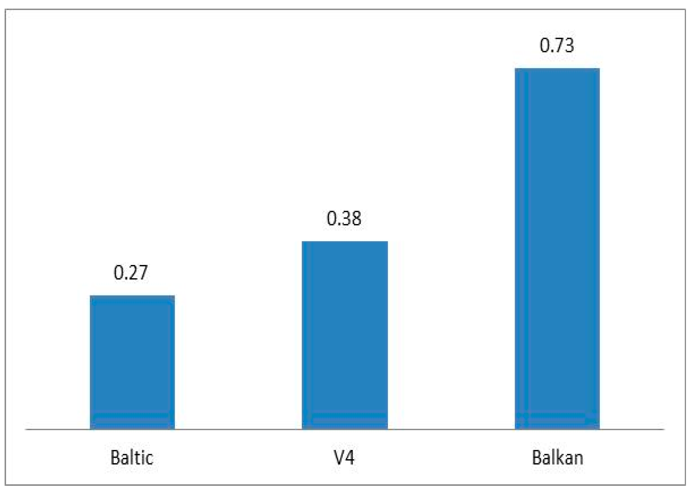
This result does not contradict the fact that the average values of efficiency (calculated by net interest margin as output) of banking systems CEE are the highest in the Balkan countries (0.67); followed by Visegrad Countries (0.385); and Baltic countries (0.25). This may indicate that banks in Balkan countries had higher net interest margin connected with weak openness of market, related to the fact that businesses have fewer opportunities to draw loans from abroad; this may be related to currency risk, which is included in the prices of products.
Several studies indicate lower efficiency of Balkan banks (Degl’Innocenti et al. 2017). That is why we did another DEA performance analysis (Efficiency2) using net loans as output. These results are consistent with other authors who claimed that more efficient banks are in V4 countries. This means that the DEA analysis with net interest margin as output is very specific and its conclusions are only valid in this context.
Additionally, Nurboja and Košak (2017) found that during the global financial crisis, the efficiency scores in South East European countries improved, which is explained by the enhanced incentives of bank managers to optimize the costs during the crisis period.
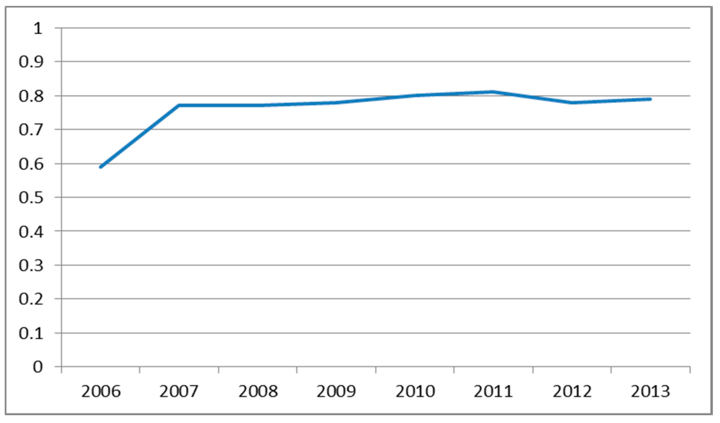
The following Figure 1 shows the average bank efficiency in specific groups of CEE countries based on Efficiency1. It was calculated for CEE banks within one dataset.
3.2. Results Related to the DEA (Data Envelope Analysis)
There are three main approaches to evaluate the efficiency of commercial banks: (1) the intermediary approach, (2) the asset-based approach, and (3) the production approach. In this paper we follow the intermediary approach.
These approaches determine the choice of inputs and outputs for the DEA models. The intermediary approach is directly based on the intermediary function of banks; the asset-based approach gives importance to the ability to build bank assets; and the third approach allows for the wide variability of inputs and outputs.
Combinations of inputs and outputs frequently used by various authors are presented in the following Table 4.
The analysis of previous papers in the field of bank efficiency shows that the most frequently used inputs were personnel expenses, deposits, capital, and fixed assets. The most frequently used outputs were credits, securities, and other earning assets.
We processed the results of an input oriented DEA model. The model inputs were net loans, customer deposits, fixed assets, and personal expenses. The output was net interest margin (NIM) because the net interest margin is an indicator that is specific for different banks. Therefore, it is the most appropriate indicator to be used for our analysis as an output of the DEA model.
The banks that were technically efficient at least once in the period 2006–2013 were marked as E in the table (see Table 5: Efficiency of individual banks). Columns 5–12 show the efficiency coefficients. These coefficients were outputs from the DEA model. The technically efficient banks have coefficient value 1; the banks with the coefficient value lower than 1 are technically not efficient. Column 1 of Table 5 indicates the number of the evaluated bank as DMU. The names of banks in the dataset are presented in Appendix of this paper (Appendix A: List of banks in the analysis). Column 2 of Table 5 shows the results of selected criteria of the association analysis. Column 3 shows the size of bank assets, column 4 expresses the efficiency of banks: efficient banks (E), or not efficient banks (N).
The following Figure 2 shows the average bank efficiency in individual CEE countries based on Efficiency1. It was calculated for CEE banks within one dataset.
We found that the average bank efficiency measured by output net interest margin was decreasing in the period of financial crisis, except Romania, Croatia, and Slovenia.
We were interested to compare the results of our research with the existing papers; thus we used a similar structure of inputs and outputs as in other studies.
In this case, for Efficiency2 the net loans were considered as outputs and customer’s deposits, fixed assets and personnel expenses were considered as inputs. This analysis is only Supplementary Information about the sensitivity of efficiency measurement to the variable considered as output. Therefore, the results of Efficiency2 are very different in comparison to Efficiency1 and the interpretation of efficiency should be in a close link to the defined starting points. The results of Efficiency2 are in the following Table 6.
The Figure 3 and Figure 4 show the differences in efficiency value due to a changed variable in the position of output.
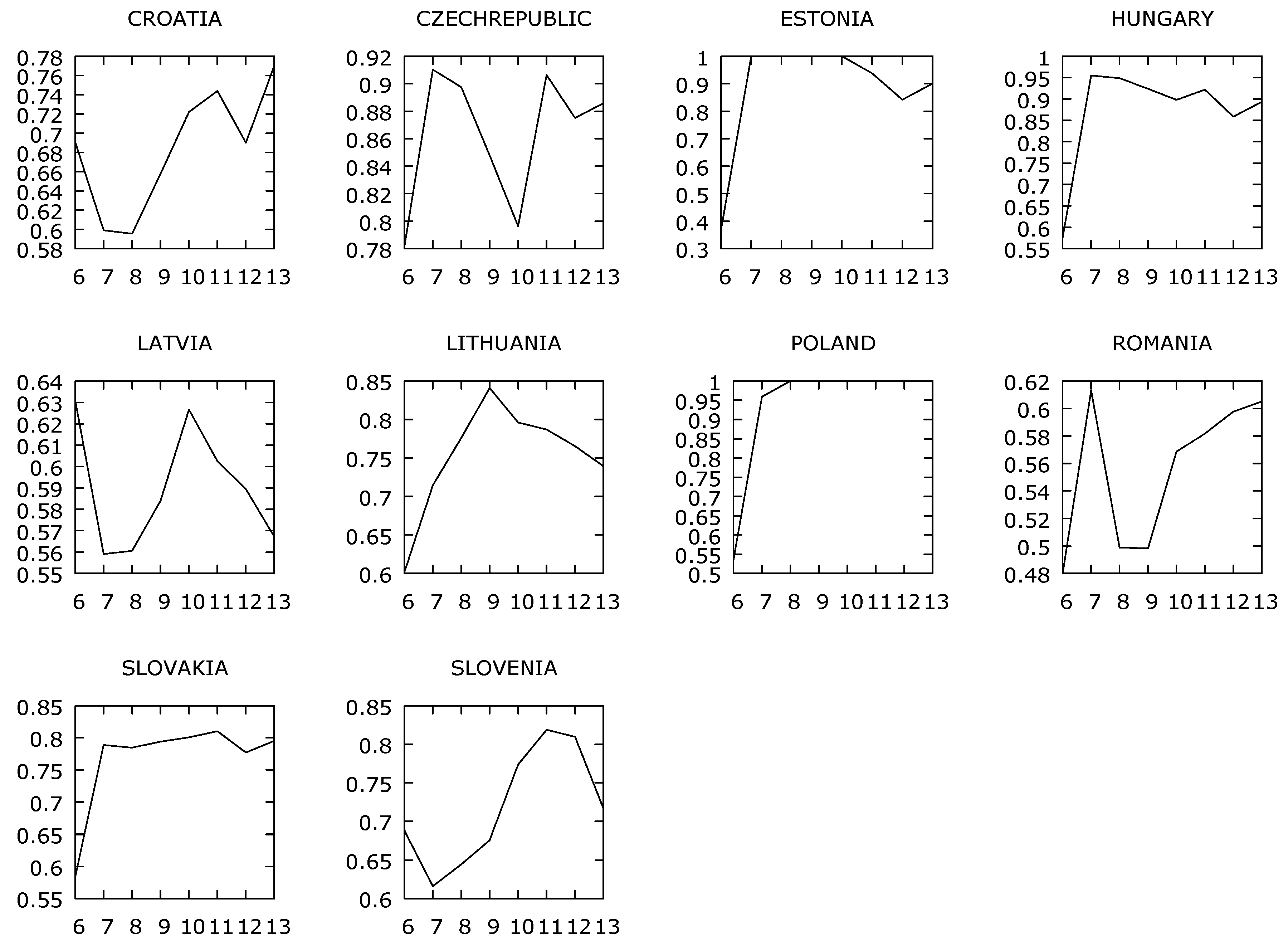
The following Figure 5 shows the average bank efficiency in individual CEE countries based on Efficiency2. It was calculated for CEE banks within one dataset.
These results are consistent with Anayiotos et al. (2010). They found that banks have the highest efficiency in the pre-crisis year of 2007.
Our results for V4 were similar to Pancurova and Lyocsa (2013), who used the mediation approach. The results for the period 2005–2008 found the banking sector in the Czech Republic as the most efficient and the banking sector in Hungary as the least efficient.
Gallizo et al. (2017) analyzed the evolution of banking efficiency in the Baltic countries after their accession to the EU and during the financial crisis. They estimated profit and cost efficiency during the period 2000–2013 using Bayesian stochastic frontier model. They found that the Baltic banking system recovered its profit efficiency very quickly after the financial crisis. The results of our efficiency analysis are consistent with this result.
We also found that the average efficiency of banks measured by BCC models in V4 countries in the period 2006–2013 ranged from 0.6 to 0.8; this result was similar to Palečková (2015); Svitalkova (2014); Anayiotos et al. (2010).
3.3. Regression Investigation
There are some differences in the efficiency of banks among the different groups of countries. We were interested in finding out what the links are between the selected factors on the one hand and the links between the technical efficiency pursued on the other hand. We tried to complete the results of DEA analysis with results of panel regression models. Data used in panel regression model are identical to the data in the DEA model. The panel regression model was estimated in the “R-studio” system.
In the next analysis, we focused on the dependence between the technical efficiency of banks (Efficiency1 with output net interest margin) as a dependent variable and the selected indicators in the countries of CEE and in individual groups of countries during the financial crisis.
In V4 countries, the results proved that there was a significant link between technical efficiency and customer’s deposits. There is a positive relationship between the technical efficiency of banks and total assets; there is a negative relationship between technical efficiency and net loans. The banks in V4 countries thus achieved efficiency from other types of assets than loans. This result shows that the negative relationship between efficiency and loans is consistent with Pancurova and Lyocsa (2013).
It is interesting to see that there is a positive relation between efficiency and loan impairment charge. It is necessary to understand the problem of “impairment” in order to understand this relationship. The international accounting principles define the “impairment” as only in the eye of the beholders. The value must be tested (at least annually) to determine if the recorded value is greater in comparison to fair value. If the fair value is lower than the recorded value, the value of loans must be charged off. Loan impairment charge is not the same as non-performing loans, but it decreases the market (fair) value of loans. So, in this sample, the loan impairment charge was positively related to efficiency.
The following Table 7 shows the results of panel regression model created for V4 countries; the dependent variable was Efficiency1.
The relationship between the technical efficiency of banks in Baltic countries as a dependent variable and gross loans is negative. This is probably connected with the period of financial crisis. Total assets have a positive relationship with the technical efficiency during the financial crisis. Pretax profit does not have a positive relationship with the technical efficiency; profitability does not automatically mean efficiency in this group of countries.
Loan Impairment Charge was in a negative relation with technical efficiency in the group of Baltic countries. Personnel expenses and fixed assets are the factors which had a negative impact on the efficiency of Baltic banks.
The following Table 8 shows the results of panel regression model created for Baltic countries; the dependent variable was Efficiency1.
The Balkan countries analysis points out that there is a negative relation between the technical efficiency as a dependent variable and the total assets. The technical efficiency of banks had a negative relation with the net loans and with the fixed assets share on total assets. The share of deposits in the liabilities had a positive impact on efficiency.
There is a negative relation between the fixed assets to total assets ratio and technical efficiency, which indicates the inappropriate range of fixed costs.
The following Table 9 shows the results of panel regression model created for Balkan countries; the dependent variable was Efficiency1.
The relationship between the technical efficiency of banks within the whole group of CEE countries and the customer deposits is positive and significant in the period of financial crisis.
The relationship between the technical efficiency on the one hand and total assets and net loans on the other hand is negative.
Personnel expenses have a positive relationship with the technical efficiency of banks in CEE countries. The causes will be the subject of the following research.
The following Table 10 shows the results of panel regression model created for the whole group of Central and Eastern Europe countries; the dependent variable was Efficiency1.
4. Conclusions
In our analysis, the technical efficiency of banks in CEE countries refers to the risk that the banks’ interest margins during the financial crisis were not adequate compared to the inputs in the form of loans, deposits, fixed assets, and personnel expenses. It could signal that there were general problems in creation of banking net interest margins during the financial crisis, especially in conditions of low interest rates policy combined with a decline in credit volumes.
The results of the association analysis show that there is a strong association between the number of efficient banks and belonging of efficient banks to the group of V4 countries. Foreign banks from Austria, Italy, and Hungary are the major bank owners. The belonging in a group of Balkan banks has not an association with the number of efficient banks in this group. There is a weak association between the number of efficient banks and belonging to the group of banks in Baltic countries.
This result does not contradict the fact that the average values of efficiency (calculated by net interest margin as output) of banking systems CEE were the highest in Balkan countries (0.67); followed by Visegrad Countries (0.385); and Baltic countries (0.25). This may indicate that banks in Balkan countries had a higher net interest margin connected with weak openness of market, related to the fact that businesses have fewer opportunities to draw loans from abroad; this may be related to currency risk, which is included in the prices of products.
We were interested to compare the results of our research with the existing papers; we used similar inputs and outputs as other studies. The net loans were considered as outputs and inputs were customer’s deposits, fixed assets, and personnel expenses. This analysis presented only Supplementary Information about the sensitivity of efficiency measurement to the variable considered as output. The results of Efficiency2 are very different in comparison to Efficiency1. Using credits as output, the average efficiency value was higher. It means that efficiency results should be explained in a close link to the defined starting points.
The association between the bank efficiency and the size of the bank assets is weak. This is an interesting result because there are higher expectations related to large banks and the current regulation protects large banks more to avoid potential negative impacts and as well as the domino effect on the entire economy.
The results of panel regression models for V4 countries show that technical efficiency is positively influenced by the customer deposits and total assets. The technical efficiency of banks had a negative relation with the net loans and the gross loans. The banks in Balkan countries thus achieved efficiency from other types of assets than loans. Total assets in the banks of Baltic countries have a negative relationship with the technical efficiency during the financial crisis.
The relationship between the technical efficiency of banks within the whole group of CEE countries and among the customer deposits is positive and significant.
Based on this analysis we can draw a conclusion that the customer deposits in CEE had a positive impact on the bank’s technical efficiency during the financial crisis. However, this result of the study will be further examined.
The results for regulators and policymakers in the area of regulation and support of credit activities are the following: it appears that the slowdown in credit activities in the sphere of the real economy has a significant impact on the banking sector. Actions to support lending activities are needed. Individual measures in the regulation should act countercyclically. Countercyclical regulation of banking sector is the right way. It is necessary to encourage banks to control risk mitigation as well as to promote the business of banks. It is particularly important to maintain the stability of the banking sector during a financial crisis.
Supplementary Materials
The following are available online at https://www.mdpi.com/2227-7072/6/3/66/s1.
Acknowledgments
I would like to thank the two anonymous reviewers who gave me valuable advice, suggestions and comments that have increased my knowledge and significantly improved this article so that I can contribute to the interesting debate on efficiency of banks in CEE countries. The contribution was created in the framework of the European Union Project entitled “Creating an Excellent Center for Economic Research for the Challenge of Civilization Challenges in the 21st Century” (ITMS 26240120032) “We support research activities in Slovakia”/the project is co-financed from EU sources, project MUNI/A/0753/2017, and project SCIEX 14.028. All support is greatly acknowledged.
Conflicts of Interest
The author declares no conflicts of interest.
Appendix A. List of Banks in the Analysis
Hrvatska Postanska Bank DD (CROATIA), Hypo Alpe-Adria-Bank dd (CROATIA), Partner Banka dd (CROATIA), Podravska Banka (CROATIA), Societe Generale—Splitska Banka dd (CROATIA), Veneto Banka d.d. (CROATIA), Zagrebacka Banka dd (CROATIA), Expobank CZ a.s. (CZECH REPUBLIC), SEB Bank (ESTONIA), Magyar Cetelem Bank Rt (HUNGARY), OTP Bank Plc (HUNGARY), ABLV Bank AS (LATVIA), As PrivatBank (LATVIA), AS DNB Banka (LATVIA), Baltic International Bank-Baltijas Starptautiska Banka (LATVIA), Jsc Latvian Development Financial Institution Altum (LATVIA), Meridian Trade Bank AS (LATVIA), Norvik Banka (LATVIA), Rietumu Banka (LATVIA), SEB banka AS (LATVIA), AB DNB Bankas (LITHUANIA), AB SEB Bankas (LITHUANIA), Citadele Bankas AB (LITHUANIA), Danske Bank A/S (LITHUANIA), Siauliu Bankas (LITHUANIA), Swedbank AB (LITHUANIA), UAB Medicinos Bankas (LITHUANIA), RBS Bank (POLAND) SA, SGB Bank SA (POLAND), Alpha Bank Romania (ROMANIA), Banca Romaneasca S.A. (ROMANIA), Bancpost SA (ROMANIA), OTP Bank Romania SA (ROMANIA), Prima banka Slovensko a.s. (SLOVAKIA), Gorenjska Banka d.d. Kranj (SLOVENIA), Nova Kreditna Banka Maribor d.d. (SLOVENIA), Raiffeisen Banka dd (SLOVENIA), SKB Banka DD (SLOVENIA), UniCredit Banka Slovenija d.d. (SLOVENIA), Komercni Banka (CZECH REPUBLIC), Ceska Sporitelna a.s. (CZECH REPUBLIC), CSOB CZ (CZECH REPUBLIC), J&T Banka a.s. (CZECH REPUBLIC), Unicredit Bank Czech Republic (CZECH REPUBLIC), VUB (SLOVAKIA), Slovenska sporitelna (SLOVAKIA), OTP Bank Slovensko (SLOVAKIA), Tatra Banka (SLOVAKIA), Postova banka (SLOVAKIA), Sberbank Slovensko (SLOVAKIA), UniCredit Bank Slovakia (SLOVAKIA).
References
- Ahmad, Rubi, Mohamed Ariff, and Michael J. Skully. 2008. Determinants of bank capital ratios in a developing economy. Asia-Pacific Financial Markets 15: 255–72. [Google Scholar] [CrossRef]
- Alqahtani, Faisal, David G. Mayes, and Kym Brown. 2017. Islamic bank efficiency compared to conventional banks during the global crisis in the GCC region. Journal of International Financial Markets, Institutions and Money 51: 58–74. [Google Scholar] [CrossRef]
- Altmann, Thomas Caspar. 2006. Cross-Border Banking in Central and Eastern Europe: Issues and Implications for Supervisory and Regulatory Organization on the European Level. Working Papers and other Publications Series Library of Congress. Working Paper 06–16; Philadelphia, PA, USA: University of Wharton, pp. 1–135. [Google Scholar]
- Anayiotos, George, Hovhannes Toroyan, and Athanasios Vamvakidis. 2010. The efficiency of emerging Europe’s banking sector before and after the recent economic crisis. Financial Theory and Practice 34: 247–67. [Google Scholar]
- Andries, Alin Marius, and Bogdan Capraru. 2014. Convergence of Bank Efficiency in Emerging Markets: The Central and Eastern European Countries’ Experience (July 21, 2012). Emerging Markets Finance and Trade 50: 31. Available online: https://ssrn.com/abstract=2135506 (accessed on 25 October 2017). [CrossRef]
- Berger, Allen N., Robert DeYoung, Mark Flannery, David Lee, and Özde Öztekin. 2008. How do large banking organizations manage their capital ratios? Journal of Financial Services Research 34: 123–49. [Google Scholar] [CrossRef]
- Égert, Balázs, Peter Backé, and Tina Zumer. 2006. Credit Growth in Central and Eastern Europe: New (over) Shooting Stars? Working Paper Series 687; Frankfurt, Germany: European Central Bank. [Google Scholar]
- Cooper, William W., Lawrence M. Seiford, and Kaoru Tone. 2007. Data Envelopment Analysis: A Comprehensive Text with Models, Applications, References and DEA-Solver Software, 2nd ed. Cham: Springer International Publishing, ISBN 10-0-387-45281-8. [Google Scholar]
- Degl’Innocenti, Marta, Stavros A. Kourtzidis, Zeljko Sevic, and Nickolaos G. Tzeremes. 2017. Investigating bank efficiency in transition economies: A window-based weight assurance region approach. Economic Modelling 67: 23–33. [Google Scholar] [CrossRef] [Green Version]
- Diallo, Boubacar. 2018. Bank efficiency and industry growth during financial crises. Economic Modelling 68: 11–22. [Google Scholar] [CrossRef]
- Distinguin, Isabelle, Caroline Roulet, and Amine Tarazi. 2013. Bank regulatory capital and liquidity: Evidence from US and European publicly traded banks. Journal of Banking & Finance, Elsevier 37: 3295–17. [Google Scholar] [CrossRef] [Green Version]
- Doan, Anh-Tuan, Kun-Li Lin, and Shuh-Chyi Doong. 2018. What drives bank efficiency? The interaction of bank income diversification and ownership. International Review of Economics & Finance 55: 203–19. [Google Scholar] [CrossRef]
- Fernandes, Filipa Da Silva, Charalampos Stasinakis, and Valeriya Bardarova. 2018. Two-stage DEA-Truncated Regression: Application in banking efficiency and financial development. Expert Systems with Applications 96: 284–301. [Google Scholar] [CrossRef]
- Gallizo, José Luis, Jordi Moreno, and Manuel Salvador. 2017. The Baltic banking system in the enlarged European Union: the effect of the financial crisis on efficiency. Baltic Journal of Economics 18: 1–24. [Google Scholar] [CrossRef]
- Gropp, Reint, and Florian Heider. 2010. The determinants of bank capital structure. Review of Finance 14: 587–622. [Google Scholar] [CrossRef]
- Halkos, E. George, and Dimitrios S. Salamouris. 2004. Efficiency measurement of the Greek commercial banks with the use of financial ratios: A data envelopment analysis approach. Management Accounting Research 15: 201–24. [Google Scholar] [CrossRef]
- Hasan, Iftekhar, and Katherin Marton. 2003. Development and Efficiency of the Banking Sector in a Transitional Economy: Hungarian Experience. Journal of Banking & Finance 27: 2249–71. [Google Scholar] [CrossRef]
- Jablonský, Josef, and Martin Dlouhý. 2004. Modely hodnocení efektivnosti produkčních jednotek. Praha: Professional Publishing, ISBN 80-86419-49-5. [Google Scholar]
- Jokipii, Terhi, and Alistair Milne. 2011. Bank Capital Buffer and Risk Adjustment Decisions. Journal of Financial Stability 7: 165–78. [Google Scholar] [CrossRef]
- Košak, Marko, and Peter Zajc. 2006. Determinants of Bank Efficiency Differences in the New EU Member Countries. Financial Stability Report, Expert Papers. Ljubljana: Bank of Slovenia. [Google Scholar]
- Matoušek, Roman, and Anita Taci. 2004. Efficiency in Banking: Empirical Evidence from the Czech Republic. Economic Change and Restructuring 37: 225–44. [Google Scholar] [CrossRef]
- Molnar, Márgit, and Daniel Holló. 2011. How Efficient Are Banks in Hungary? OECD Economics Department Working Papers 848. Paris, France: OECD Publishing. [Google Scholar]
- Novickytė, Lina, and Jolanta Droždz. 2018. Measuring the Efficiency in the Lithuanian Banking Sector: The DEA Application. International Journal of Financial Studies 6: 37. [Google Scholar] [CrossRef]
- Nurboja, Bashkim, and Marko Košak. 2017. Banking efficiency in South East Europe: Evidence for financial crises and the gap between new EU members and candidate countries. Economic Systems 41: 122–38. [Google Scholar] [CrossRef]
- Palečková, Iveta. 2015. Banking Efficiency in Visegrad Countries: A Dynamic Data Envelopment Analysis. Acta Universitatis Agriculturae et Silviculturae Mendelianae Brunensis 63: 2085–91. [Google Scholar] [CrossRef]
- Pancurova, Dana, and Stefan Lyocsa. 2013. Determinants of Commercial Banks’ Efficiency: Evidence from 11 CEE Countries. Finance a Uver—Czech Journal of Economics and Finance 63: 152–79. [Google Scholar]
- Řepková, Iveta. 2014. Estimation of Banking Efficiency in the Czech Republic: Dynamic Data Envelopment Analysis. Danube 4: 261–75. [Google Scholar] [CrossRef]
- Stavárek, Daniel. 2005. Restrukturalizace bankovních sektorů a efektivnost bank v zemích Visegrádské skupiny. Karviná: Slezská univerzita, Obchodně podnikatelská fakulta, ISBN 80-7248-319-6. [Google Scholar]
- Svitalkova, Zuzana. 2014. Comparison and Evaluation of Bank Efficiency in Austria and the Czech Republic. Journal of Competitiveness 6: 15–29. [Google Scholar] [CrossRef] [Green Version]
- Tanda, Alessandra. 2015. The Effects of Bank Regulation on the Relationship Between Capital and Risk. Comparative Economic Studies, Palgrave Macmillan; Association for Comparative Economic Studies 57: 31–54. [Google Scholar] [CrossRef] [Green Version]
- Toloo, Mehdi, Maryam Allahyar, and Jana Hančlová. 2018. A non-radial directional distance method on classifying inputs and outputs in DEA. Expert Systems with Applications 92: 495–506. [Google Scholar] [CrossRef]
- VanHoose, David. 2007. Theories of bank behavior under capital regulation. Journal of Banking & Finance 31: 3680–97. [Google Scholar]
- Woznievska, Grazyna. 2008. Methods of Measuring the efficiency of Commercial Banks. An Example of Polish Banks. Ekonomika 84: 81–89. [Google Scholar]
- Zimková, Emília. 2014. Technical Efficiency and Super-Efficiency of the Banking Sector in Slovakia. Paper presented at Enterprise and the Competitive Environment 2014 Conference (ECE), Brno, Czech Republic, March 6–7; pp. 780–87. [Google Scholar]
Figure 1.
Average Efficiency1 of V4, Baltic and Balkan countries. Source: Author’s own processing.

Figure 2.
Average Efficiency1 banks in CEE countries. Source: Author’s own processing. The years on the x-axis are marked as follows: 2006 as “6”, 2007 as “7”, 2008 as “8”, 2009 as “9”, 2010 as “10”, 2011 as “11”, 2012 as “12” and the year 2013 as “13”.
Figure 2.
Average Efficiency1 banks in CEE countries. Source: Author’s own processing. The years on the x-axis are marked as follows: 2006 as “6”, 2007 as “7”, 2008 as “8”, 2009 as “9”, 2010 as “10”, 2011 as “11”, 2012 as “12” and the year 2013 as “13”.
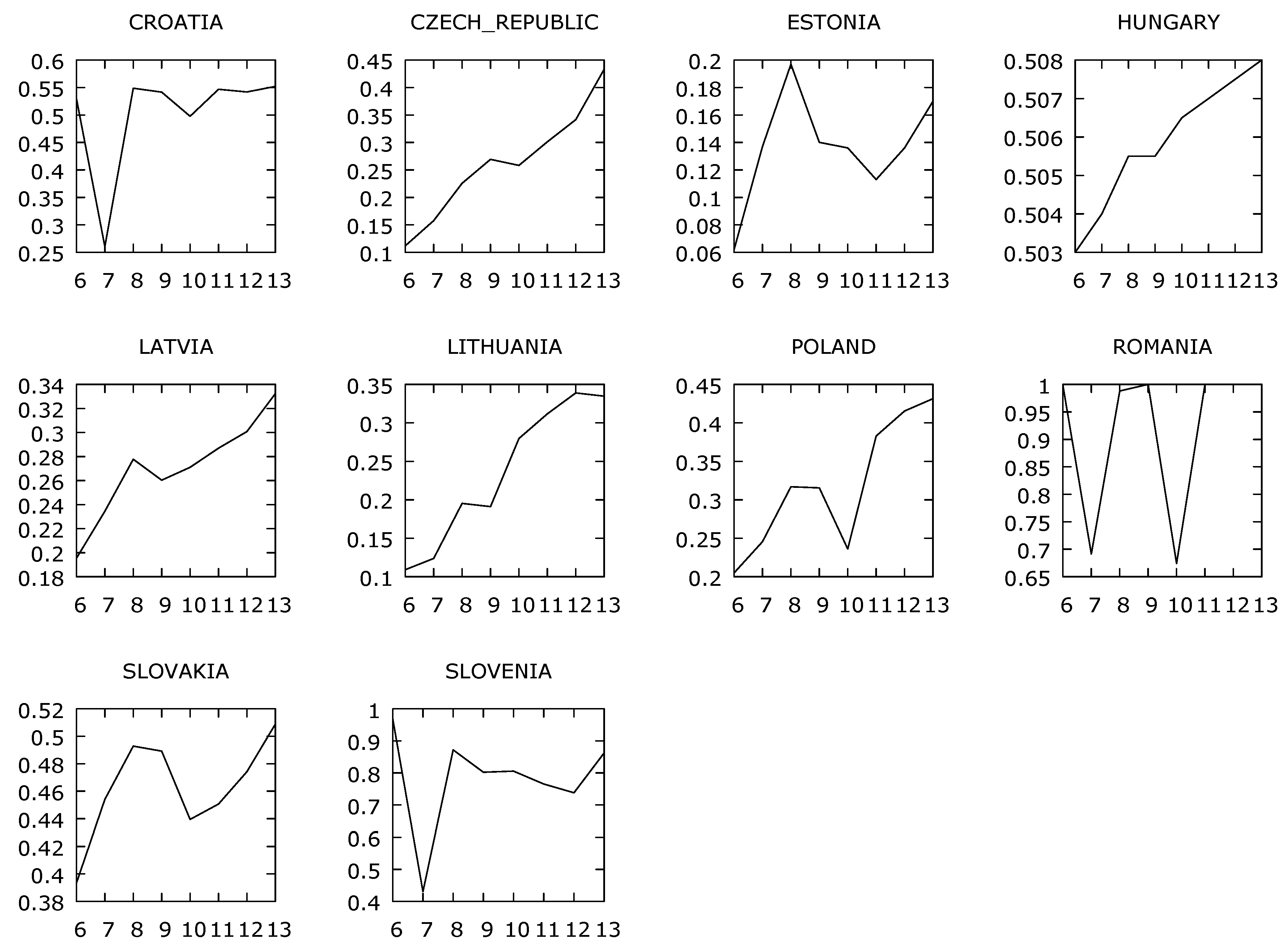
Figure 3.
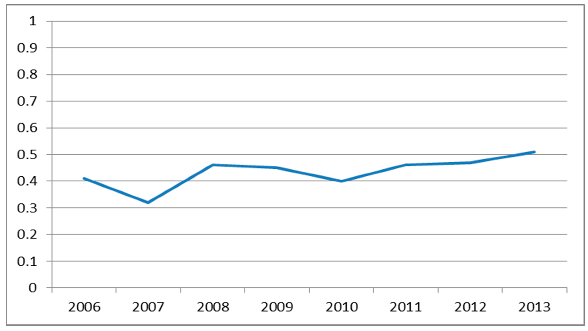
Average efficiency of banks in CEE countries in the time period 2006–2013 using output net interest margin. Source: processing using data from BankScope.
Figure 3.
Average efficiency of banks in CEE countries in the time period 2006–2013 using output net interest margin. Source: processing using data from BankScope.

Figure 4.
Average efficiency of banks in CEE countries in the time period 2006–2013 using output net loans. Source: processing using data from BankScope
Figure 4.
Average efficiency of banks in CEE countries in the time period 2006–2013 using output net loans. Source: processing using data from BankScope

Figure 5.
Average Efficiency2 banks in CEE countries. Source: processing using data from BankScope. The years on the x-axis are marked as follows: 2006 as “6”, 2007 as “7”, 2008 as “8”, 2009 as “9”, 2010 as “10”, 2011 as “11”, 2012 as “12” and the year 2013 as “13”.
Figure 5.
Average Efficiency2 banks in CEE countries. Source: processing using data from BankScope. The years on the x-axis are marked as follows: 2006 as “6”, 2007 as “7”, 2008 as “8”, 2009 as “9”, 2010 as “10”, 2011 as “11”, 2012 as “12” and the year 2013 as “13”.

Table 1.
Variables and descriptive statistics.
| Variable (408 obs.) | Mean | Std. Dev. | Min | Max |
|---|---|---|---|---|
| Net_Loans | 3,330,957 | 5,200,090 | 33,200 | 2.52 × 10⁷ |
| Fixed_Assets | 72,704.41 | 143,895.4 | 203.5802 | 854,087.8 |
| Total_Assets | 6,007,096 | 1.03 × 10⁷ | 50,900 | 5.12 × 10⁷ |
| Customer_Deposits | 3,862,094 | 7,310,269 | 2355.137 | 3.57 × 10⁷ |
| Loan_Impairement_Charge | 68,879.19 | 337,403.1 | −80,600 | 4,057,277 |
| Pretax_Profit | 74,459.27 | 205,241.8 | −616,300 | 1,082,099 |
| Net_Interest_Margin | 2.511416 | 1.199684 | −0.634 | 7.75 |
| Personnel_Expenses | 63,276.83 | 144,561.1 | 1400 | 1,613,941 |
| Efficiency | 0.4267819 | 0.3941406 | 0.006 | 1 |
| FAtoTA | 0.0151592 | 0.0259411 | 0.0001375 | 0.3438067 |
| NLtoCD | 2.802042 | 11.08168 | 0.1620511 | 118.7907 |
| NLtoTA | 0.6102892 | 0.1542593 | 0.0527622 | 0.9532463 |
| CDtoLI | 0.5912198 | 0.2091098 | 0.0076442 | 0.9053834 |
| LICHtoNL | 0.0186461 | 0.0321562 | −0.0709684 | 0.2544897 |
| PEtoPP | 0.0117172 | 0.0058037 | 0.0013766 | 0.0352589 |
Table 2.
Results of efficiency1 related to the size of banks.
| Criteria | χ2 Value | H0 |
|---|---|---|
| Size of the bank (large or small) | 2.63 | Not rejection H0; There is no association |
Source: processing using data from BankScope.
Table 3.
Results for banks belonging to different groups of Central and Eastern European (CEE) countries related to number of efficient banks in the group of countries.
Table 3.
Results for banks belonging to different groups of Central and Eastern European (CEE) countries related to number of efficient banks in the group of countries.
| Criteria | χ2 Value | H0 |
|---|---|---|
| V4 Countries (Slovakia, Czech Republic, Hungary, Poland) | 9.71 | Rejection of H0; There is an association. |
| Baltic Countries (Estonia, Latvia, Lithuania) | 1.55 | Not rejection H0; There is no association. |
| Balkan Countries (Croatia, Slovenia, Romania) | 5.30 | Rejection of H0; There is an association. |
Source: processing using data from BankScope.
Table 4.
Comparison of input and output combinations in selected papers.
| Fernandes et al. (2018) | Nurboja and Košak (2017) | Degl’Innocenti et al. (2017) | Halkos and Salamouris (2004) | Stavárek (2005) | Molnar and Holló (2011) | Pancurova and Lyocsa (2013) | Zimková (2014) | Palečková (2015) | Toloo et al. (2018) | Diallo (2018) | Novickytė and Droždz (2018) | |
|---|---|---|---|---|---|---|---|---|---|---|---|---|
| Inputs | ||||||||||||
| Fixed Assets | x | x | ||||||||||
| Personnel Expenses | x | x | x | x | x | x | x | x | ||||
| Equity | x | x | x | |||||||||
| Deposits | x | x | x | x | x | x | ||||||
| Number of Employees | x | |||||||||||
| Total Assets | x | |||||||||||
| Total Costs | x | |||||||||||
| Borrowed Funds | x | |||||||||||
| Physical Capital (property) | x | |||||||||||
| Interest Costs | x | x | ||||||||||
| Operating Costs | x | |||||||||||
| Financial Efficiency Ratios | x | |||||||||||
| Credit Risk | x | |||||||||||
| Variable position of inputs and outputs | ||||||||||||
| Deposits | x | x | x | |||||||||
| Outputs | ||||||||||||
| Credits | x | x | x | x | x | x | x | x | x | X | ||
| Securities | x | x | x | x | ||||||||
| Other Earning Assets | x | x | x | |||||||||
| Investments | x | X | ||||||||||
| Profit | x | |||||||||||
| Total Income | x | |||||||||||
| ROA (Return to Assets) | x | |||||||||||
| Net Interest Income | x | x | ||||||||||
| Non-Interest Income | x | x | ||||||||||
| Net Interest Margin | x | |||||||||||
| Financial Efficiency Ratios | x |
Source: Author’s own processing.
Table 5.
Efficiency1 of individual banks (net interest margin as an output).
| Bank Nr. | Large (L)/Small (S) Bank | Assets (Thous. EUR) | Efficient (E) Non-Efficient (N) | 2006 | 2007 | 2008 | 2009 | 2010 | 2011 | 2012 | 2013 | Average Efficiency of the Bank |
|---|---|---|---|---|---|---|---|---|---|---|---|---|
| 1 | 2 | 3 | 4 | 5 | 6 | 7 | 8 | 9 | 10 | 11 | 12 | 13 |
| 1 | S | 2,398,762 | N | 0.041 | 0.051 | 0.058 | 0.072 | 0.083 | 0.088 | 0.093 | 0.096 | 0.07275 |
| 2 | L | 3,919,225 | N | 0.031 | 0.041 | 0.057 | 0.036 | 0.040 | 0.039 | 0.046 | 0.053 | 0.042875 |
| 3 | S | 186,926.6 | N | 0.324 | 0.460 | 0.671 | 0.841 | 0.774 | 0.788 | 0.860 | 0.939 | 0.707125 |
| 4 | S | 405,488.9 | N | 0.174 | 0.248 | 0.362 | 0.474 | 0.404 | 0.394 | 0.416 | 0.442 | 0.36425 |
| 5 | L | 3,570,356 | N | 0.021 | 0.029 | 0.042 | 0.043 | 0.053 | 0.057 | 0.065 | 0.070 | 0.0475 |
| 6 | S | 203,417.4 | E | 1.000 | 1.000 | 1.000 | 1.000 | 1.000 | 1.000 | 1.000 | 1.000 | 1 |
| 7 | L | 13,917,242 | N | 0.006 | 0.008 | 0.011 | 0.011 | 0.013 | 0.014 | 0.015 | 0.016 | 0.01175 |
| 8 | S | 1,146,893 | N | 0.056 | 0.084 | 0.103 | 0.113 | 0.117 | 0.124 | 0.123 | 0.139 | 0.107375 |
| 9 | L | 4,002,900 | N | 0.080 | 0.114 | 0.146 | 0.141 | 0.124 | 0.097 | 0.091 | 0.098 | 0.111375 |
| 10 | S | 274,907 | E | 1.000 | 1.000 | 1.000 | 1.000 | 1.000 | 1.000 | 1.000 | 1.000 | 1 |
| 11 | L | 22,435,283 | N | 0.008 | 0.007 | 0.010 | 0.009 | 0.011 | 0.013 | 0.013 | 0.016 | 0.010875 |
| 12 | S | 3,315,400 | N | 0.065 | 0.081 | 0.146 | 0.121 | 0.131 | 0.156 | 0.161 | 0.159 | 0.1275 |
| 13 | S | 80,5100 | N | 0.402 | 0.484 | 0.624 | 0.622 | 0.461 | 0.753 | 0.818 | 0.847 | 0.626375 |
| 14 | S | 2,311,800 | N | 0.075 | 0.103 | 0.136 | 0.132 | 0.123 | 0.108 | 0.132 | 0.144 | 0.119125 |
| 15 | S | 336,656 | E | 0.747 | 1.000 | 1.000 | 1.000 | 0.801 | 0.898 | 1.000 | 1.000 | 0.93075 |
| 16 | S | 295,800 | E | 0.079 | 0.117 | 0.164 | 0.149 | 0.194 | 0.441 | 0.569 | 1.000 | 0.339125 |
| 17 | S | 340,100 | E | 1.000 | 1.000 | 1.000 | 1.000 | 1.000 | 1.000 | 1.000 | 1.000 | 1 |
| 18 | S | 792,900 | N | 0.124 | 0.251 | 0.412 | 0.407 | 0.220 | 0.223 | 0.287 | 0.531 | 0.306875 |
| 19 | S | 2,920,500 | N | 0.063 | 0.059 | 0.157 | 0.132 | 0.152 | 0.144 | 0.181 | 0.165 | 0.131625 |
| 20 | L | 4,134,500 | N | 0.039 | 0.063 | 0.086 | 0.091 | 0.117 | 0.106 | 0.131 | 0.117 | 0.09375 |
| 21 | L | 3,486,000 | N | 0.034 | 0.039 | 0.056 | 0.057 | 0.061 | 0.061 | 0.065 | 0.067 | 0.055 |
| 22 | L | 6,837,100 | N | 0.036 | 0.056 | 0.066 | 0.060 | 0.072 | 0.075 | 0.104 | 0.089 | 0.06975 |
| 23 | S | 287,896 | N | 0.244 | 0.232 | 0.422 | 0.426 | 0.575 | 0.609 | 0.680 | 0.738 | 0.49075 |
| 24 | S | 1,401,981 | E | 0.231 | 0.282 | 0.384 | 0.390 | 0.775 | 1.000 | 1.000 | 1.000 | 0.63275 |
| 25 | S | 1,520,800 | N | 0.116 | 0.135 | 0.196 | 0.182 | 0.206 | 0.187 | 0.212 | 0.167 | 0.175125 |
| 26 | L | 5,610,150 | N | 0.019 | 0.031 | 0.039 | 0.052 | 0.061 | 0.055 | 0.062 | 0.060 | 0.047375 |
| 27 | S | 254,800 | N | 0.438 | 0.454 | 0.608 | 0.529 | 0.691 | 0.863 | 0.850 | 0.957 | 0.67375 |
| 28 | S | 810,417 | E | 0.742 | 1.000 | 1.000 | 1.000 | 1.000 | 1.000 | 1.000 | 1.000 | 0.96775 |
| 29 | S | 3,059,359 | N | 0.269 | 0.339 | 0.514 | 0.364 | 0.276 | 0.221 | 0.299 | 0.412 | 0.33675 |
| 30 | S | 3,624,832 | N | 0.037 | 0.039 | 0.044 | 0.038 | 0.044 | 0.051 | 0.063 | 0.068 | 0.048 |
| 31 | S | 1,612,257 | N | 0.081 | 0.068 | 0.082 | 0.086 | 0.097 | 0.116 | 0.140 | 0.158 | 0.1035 |
| 32 | S | 2,644,139 | N | 0.026 | 0.027 | 0.041 | 0.040 | 0.041 | 0.047 | 0.056 | 0.075 | 0.044125 |
| 33 | S | 1,027,138 | N | 0.106 | 0.108 | 0.123 | 0.187 | 0.165 | 0.141 | 0.132 | 0.148 | 0.13875 |
| 34 | S | 1,900,400 | N | 0.040 | 0.044 | 0.048 | 0.047 | 0.064 | 0.089 | 0.105 | 0.112 | 0.068625 |
| 35 | S | 1,560,900 | N | 0.062 | 0.137 | 0.197 | 0.140 | 0.136 | 0.113 | 0.136 | 0.170 | 0.136375 |
| 36 | S | 3,910,000 | N | 0.016 | 0.021 | 0.029 | 0.028 | 0.033 | 0.035 | 0.042 | 0.061 | 0.033125 |
| 37 | S | 1,186,900 | N | 0.103 | 0.133 | 0.152 | 0.126 | 0.144 | 0.142 | 0.156 | 0.188 | 0.143 |
| 38 | S | 2,451,000 | N | 0.026 | 0.040 | 0.054 | 0.054 | 0.058 | 0.059 | 0.066 | 0.073 | 0.05375 |
| 39 | S | 2,488,600 | N | 0.088 | 0.153 | 0.138 | 0.110 | 0.125 | 0.080 | 0.096 | 0.114 | 0.113 |
| 40 | L | 41,292,890 | E | 1.000 | 0.506 | 1.000 | 0.960 | 1.000 | 1.000 | 0.933 | 0.937 | 0.917 |
| 41 | L | 48,302,441 | E | 1.000 | 0.348 | 1.000 | 1.000 | 0.761 | 1.000 | 1.000 | 1.000 | 0.888625 |
| 42 | L | 49,182,578 | E | 0.962 | 0.383 | 0.949 | 1.000 | 0.898 | 1.000 | 1.000 | 1.000 | 0.899 |
| 43 | L | 4,639,270 | E | 1.000 | 0.570 | 1.000 | 1.000 | 0.253 | 1.000 | 1.000 | 1.000 | 0.852875 |
| 44 | L | 16,736,237 | E | 1.000 | 0.872 | 1.000 | 1.000 | 0.444 | 1.000 | 1.000 | 1.000 | 0.9145 |
| 45 | L | 11,151,378 | E | 1.000 | 0.323 | 0.952 | 1.000 | 1.000 | 1.000 | 1.000 | 1.000 | 0.909375 |
| 46 | L | 11,664,515 | E | 0.993 | 1.000 | 1.000 | 1.000 | 1.000 | 1.000 | 1.000 | 1.000 | 0.999125 |
| 47 | S | 1,420,781 | E | 0.972 | 0.303 | 0.790 | 0.803 | 0.817 | 0.745 | 0.728 | 1.000 | 0.76975 |
| 48 | L | 9,453,403 | E | 1.000 | 0.543 | 0.943 | 0.864 | 1.000 | 0.858 | 0.783 | 0.733 | 0.8405 |
| 49 | S | 3,843,009 | E | 1.000 | 0.636 | 1.000 | 1.000 | 1.000 | 1.000 | 1.000 | 1.000 | 0.9545 |
| 50 | S | 2,031,665 | N | 0.869 | 0.285 | 0.733 | 0.659 | 0.619 | 0.610 | 0.587 | 0.719 | 0.635125 |
| 51 | L | 15,422,623 | E | 1.000 | 0.387 | 0.895 | 0.685 | 0.592 | 0.614 | 0.592 | 0.861 | 0.70325 |
| Median | 3,919,225 | - | - | - | - | - | - | - | - | 0.426782 | ||
| Average efficiency | 0.389 | 0.307 | 0.443 | 0.436 | 0.408 | 0.455 | 0.468 | 0.504 |
Source: processing using data from BankScope. Columns 5–12 contain the efficiency coefficients of individual banks in dataset (Appendix A: List of banks in the analysis).
Table 6.
Efficiency2 of individual banks (credits volume as the output).
| Bank Nr. | Efficient (E) Not-Efficient (N) | 2006 | 2007 | 2008 | 2009 | 2010 | 2011 | 2012 | 2013 | Average Efficiency of the Bank |
|---|---|---|---|---|---|---|---|---|---|---|
| 1 | 4 | 5 | 6 | 7 | 8 | 9 | 10 | 11 | 12 | 13 |
| 1 | N | 1.0000 | 0.9976 | 1.0000 | 1.0000 | 1.0000 | 1.0000 | 0.9801 | 0.9801 | 0.9947 |
| 2 | N | 0.4684 | 1.0000 | 1.0000 | 1.0000 | 1.0000 | 1.0000 | 1.0000 | 1.0000 | 0.9335 |
| 3 | N | 0.7929 | 0.4899 | 0.4329 | 0.3534 | 0.3605 | 0.4964 | 0.6070 | 0.6027 | 0.5169 |
| 4 | N | 1.0000 | 1.0000 | 0.9523 | 0.7335 | 0.4173 | 0.9420 | 0.6635 | 0.7319 | 0.8051 |
| 5 | N | 1.0000 | 0.9739 | 1.0000 | 1.0000 | 1.0000 | 1.0000 | 1.0000 | 1.0000 | 0.9967 |
| 6 | E | 0.8606 | 1.0000 | 1.0000 | 1.0000 | 1.0000 | 1.0000 | 1.0000 | 1.0000 | 0.9826 |
| 7 | N | 0.4864 | 0.8054 | 0.9117 | 0.8697 | 0.8952 | 0.7740 | 0.6902 | 0.6015 | 0.7543 |
| 8 | N | 0.1562 | 0.4805 | 0.4686 | 0.5087 | 0.4672 | 0.5554 | 0.5556 | 0.7590 | 0.4939 |
| 9 | N | 0.4085 | 0.1343 | 0.2111 | 0.2845 | 0.3180 | 0.3887 | 0.4542 | 0.4362 | 0.3295 |
| 10 | E | 1.0000 | 0.4669 | 0.4986 | 0.5951 | 0.7337 | 0.4882 | 0.5718 | 0.6109 | 0.6206 |
| 11 | N | 0.4072 | 1.0000 | 1.0000 | 1.0000 | 1.0000 | 1.0000 | 1.0000 | 1.0000 | 0.9259 |
| 12 | N | 0.7538 | 0.4135 | 0.3943 | 0.4685 | 0.4842 | 0.6210 | 0.6003 | 0.6310 | 0.5458 |
| 13 | N | 0.6650 | 0.9182 | 1.0000 | 1.0000 | 1.0000 | 1.0000 | 1.0000 | 1.0000 | 0.9479 |
| 14 | N | 0.7368 | 0.6451 | 0.6206 | 0.7304 | 0.7654 | 0.7661 | 0.7777 | 0.7801 | 0.7278 |
| 15 | E | 1.0000 | 0.7653 | 0.7881 | 0.8183 | 0.9425 | 0.8248 | 0.8575 | 0.8331 | 0.8537 |
| 16 | E | 0.4264 | 1.0000 | 1.0000 | 1.0000 | 1.0000 | 1.0000 | 1.0000 | 1.0000 | 0.9283 |
| 17 | E | 0.6166 | 0.7868 | 0.5827 | 0.7936 | 0.7942 | 1.0000 | 0.6983 | 0.7575 | 0.7537 |
| 18 | N | 0.8237 | 0.7220 | 0.8481 | 0.9915 | 1.0000 | 0.8171 | 0.7123 | 0.8382 | 0.8441 |
| 19 | N | 1.0000 | 0.8308 | 1.0000 | 1.0000 | 0.9488 | 0.9099 | 0.8515 | 0.9129 | 0.9317 |
| 20 | N | 0.4009 | 1.0000 | 1.0000 | 1.0000 | 1.0000 | 1.0000 | 1.0000 | 1.0000 | 0.9251 |
| 21 | N | 1.0000 | 0.4654 | 0.7126 | 0.8584 | 0.6497 | 0.5256 | 0.4523 | 0.4936 | 0.6447 |
| 22 | N | 0.3432 | 1.0000 | 1.0000 | 1.0000 | 1.0000 | 1.0000 | 1.0000 | 1.0000 | 0.9179 |
| 23 | N | 0.7182 | 0.6374 | 0.6115 | 0.8810 | 0.7935 | 0.9646 | 0.8134 | 0.6385 | 0.7573 |
| 24 | E | 0.3938 | 0.7327 | 0.7327 | 0.7763 | 0.7369 | 0.7053 | 0.7617 | 0.7482 | 0.6984 |
| 25 | N | 0.3540 | 0.3345 | 0.3763 | 0.3702 | 0.4427 | 0.4043 | 0.4779 | 0.3825 | 0.3928 |
| 26 | N | 0.2402 | 0.3688 | 0.3837 | 0.3814 | 0.3373 | 0.2838 | 0.3122 | 0.2119 | 0.3149 |
| 27 | N | 1.0000 | 0.3029 | 0.3341 | 0.3614 | 0.2449 | 0.1724 | 0.1565 | 0.1735 | 0.3432 |
| 28 | E | 0.3810 | 1.0000 | 1.0000 | 1.0000 | 1.0000 | 1.0000 | 0.9946 | 0.8913 | 0.9084 |
| 29 | N | 0.5021 | 0.1452 | 0.1569 | 0.1593 | 0.2672 | 0.2534 | 0.2142 | 0.2566 | 0.2444 |
| 30 | N | 1.0000 | 0.5220 | 0.6110 | 0.5746 | 1.0000 | 0.8515 | 1.0000 | 1.0000 | 0.8199 |
| 31 | N | 0.2588 | 1.0000 | 1.0000 | 1.0000 | 1.0000 | 1.0000 | 1.0000 | 1.0000 | 0.9074 |
| 32 | N | 0.2966 | 0.3130 | 0.3152 | 0.4037 | 0.2865 | 0.2977 | 0.2605 | 0.1684 | 0.2927 |
| 33 | N | 1.0000 | 0.4267 | 0.4275 | 0.5016 | 0.5627 | 0.5638 | 0.4261 | 0.4620 | 0.5463 |
| 34 | N | 1.0000 | 0.9530 | 0.8171 | 0.8740 | 0.9405 | 1.0000 | 0.9410 | 0.9403 | 0.9332 |
| 35 | N | 0.3720 | 1.0000 | 1.0000 | 1.0000 | 1.0000 | 0.9377 | 0.8421 | 0.9007 | 0.8816 |
| 36 | N | 0.8952 | 0.3763 | 0.3565 | 0.3513 | 0.3926 | 0.4450 | 0.5366 | 0.5754 | 0.4911 |
| 37 | N | 0.3418 | 0.6838 | 0.6779 | 0.9198 | 1.0000 | 1.0000 | 0.8557 | 0.8562 | 0.7919 |
| 38 | N | 0.2338 | 0.3835 | 0.4320 | 0.4614 | 0.6445 | 0.6480 | 0.4129 | 0.8142 | 0.5038 |
| 39 | N | 0.8063 | 0.2656 | 0.2059 | 0.2287 | 0.3166 | 0.4116 | 0.3687 | 0.4681 | 0.3839 |
| 40 | E | 1.0000 | 0.6062 | 0.5797 | 0.6433 | 0.7001 | 0.7026 | 0.6568 | 0.6762 | 0.6956 |
| 41 | E | 1.0000 | 1.0000 | 1.0000 | 1.0000 | 1.0000 | 1.0000 | 1.0000 | 1.0000 | 1.0000 |
| 42 | E | 0.5578 | 0.8780 | 0.9165 | 1.0000 | 1.0000 | 1.0000 | 1.0000 | 1.0000 | 0.9190 |
| 43 | E | 0.5261 | 0.7536 | 0.7343 | 0.9267 | 1.0000 | 1.0000 | 1.0000 | 1.0000 | 0.8676 |
| 44 | E | 0.5337 | 0.5396 | 0.5525 | 0.4172 | 0.5225 | 0.5249 | 0.5205 | 0.5364 | 0.5184 |
| 45 | E | 0.5378 | 0.6937 | 0.4176 | 0.4104 | 0.4992 | 0.4932 | 0.5101 | 0.4849 | 0.5058 |
| 46 | E | 0.3227 | 0.4655 | 0.2911 | 0.2387 | 0.2526 | 0.3088 | 0.3601 | 0.3994 | 0.3299 |
| 47 | E | 0.6277 | 0.4899 | 0.5313 | 0.5560 | 0.6080 | 0.6985 | 0.6684 | 0.6092 | 0.5986 |
| 48 | E | 0.3893 | 0.6241 | 0.6020 | 0.6566 | 0.7398 | 0.7518 | 0.6845 | 0.5333 | 0.6227 |
| 49 | E | 0.6414 | 0.5248 | 0.5725 | 0.6149 | 0.7923 | 0.9148 | 0.9781 | 0.9002 | 0.7424 |
| 50 | N | 0.7837 | 0.6231 | 0.6347 | 0.6659 | 0.7281 | 0.7289 | 0.7486 | 0.7097 | 0.7028 |
| 51 | E | 1.0000 | 0.8186 | 0.8820 | 0.8849 | 1.0000 | 1.0000 | 0.9691 | 0.8305 | 0.9231 |
| Average | 0.6482 | 0.6737 | 0.6779 | 0.7111 | 0.7370 | 0.7485 | 0.7244 | 0.7282 | 0.7061 |
Source: processing using data from BankScope. Columns 5–12 contain the efficiency coefficients of individual banks in dataset (Appendix A: List of banks in the analysis).
Table 7.
Results of panel regression model for V4 countries (dependent variable Efficiency1).
| Model 1 “Pooling” | Model 2 “Pooling” | Model 3 “Pooling” | Model 4 “Pooling” | Model 5 “Pooling” | Model 6 “Pooling” | Model 7 “Pooling” | |
|---|---|---|---|---|---|---|---|
| (Intercept) | 13.957 * (6.584) (2.119) | 34.62 *** (5.542) (6.247) | 10.729 (6.896) (1.555) | 21.839 ** (6.67) (3.274) | 28.016 *** (5.548) (5.049) | 47.287 *** (4.549) (10.393) | 29.21 *** (5.993) (4.874) |
| Net_Loans | −0.159 ** (0.053) (6.247) | −0.1322 * (0.055) (−2.397) | |||||
| Total_Assets | 0.1838 *** (0.047) (3.983) | 0.1629 ** (0.049) (3.323) | 0.1725 *** (0.049) (3.510) | 0.1764 *** (0.049) (−0.538) | |||
| Customer_Deposits | 0.2488 *** (0.048) (5.184) | 0.288 *** (0.053) (5.388) | 0.2405 *** (0.048) (5.002) | 0.242 *** (0.05) (4.804) | 0.227 *** (0.049) (4.587) | 0.2565 *** (0.055) (4.654) | 0.2328 *** (0.051) (4.596) |
| Personnel_Expenses | 0.0740 (0.049) (1.505) | ||||||
| Loan_Impairment_Charge | 0.1703 *** (0.046) (3.629) | 0.178 *** (0.048) (3.697) | 0.1725 *** (0.049) (3.690) | 0.150 ** (0.048) (3.083) | |||
| Fixed_Assets | −0.026 (0.026) (−0.538) | ||||||
| R-Squared: | 0.243 | 0.212 | 0.255 | 0.184 | 0.172 | 0.134 | 0.173 |
| F-statistic: | 14.979 | 12.526 | 11.902 | 10.560 | 14.623 | 10.970 | 9.796 |
Source: processing using data from BankScope. Values in parentheses are std. error and t-value and *** denotes statistical significance at the 1% level, ** at the 5% level and * at the 10% level.
Table 8.
Results of panel regression model for the Baltic Countries (dependent variable Efficiency).
Table 8.
Results of panel regression model for the Baltic Countries (dependent variable Efficiency).
| Model 1 “Fixed” | Model 2 “Fixed” | Model 3 “Pooling” | Model 4 “Fixed” | Model 5 “Pooling” | Model 6 “Random” | Model 7 “Fixed” | |
|---|---|---|---|---|---|---|---|
| Intercept | - | 90.121 *** 11.782 7.648 | 93.215 *** (11.219) (8.308) | 47.700 *** (9.867) (4.834) | |||
| Total_Assets | 0.1414 ** (0.043) (3.240) | 0.152 *** (0.043) (3.495) | 0.1429 ** (0.044) | 0.146 ** (0.044) 3.308 | 0.1455 (0.083) (−2.94) | 0.118 ** (0.044) (2.636) | 0.138 ** (0.044) (3.097) |
| Gross_Loans | −0.076 * (0.035) (−2.124) | −0.077 * (0.036) (−2.137) | −1.158 * 0.068 −2.303 | −0.071 (0.036) −1.926 | −0.151 * (0.067) (−2.238) | −0.077 * (0.036) (−1.892) | −0.069 0.036 −1.892 |
| Common_Equity | 0.0701 (0.043) (1.629) | −0.193 * (0.085) (−2.249) | 0.033 (0.043) (0.773) | 0.048 (0.043) (1.119) | |||
| Personnel_Expenses | −0.061 (0.047) (−1.277) | −0.061 (0.047) (−1.286) | −0.174 * (0.082) (2.120) | −0.072 (0.048) (−1.485) | −0.197 * (0.081) (2.418) | −0.055 (0.048) (−1.129) | −0.072 (0.048) (−1.494) |
| Loan_Impairment_Charge | −0.010 (0.031) −0.349) | −0.226 (0.030) | −0.052 (0.077) −0.677 | −0.0102 (0.030) (−0.335) | −0.076 (0.076) (−0.996) | −0.006 (0.032) (−0.192) | −0.00095 (0.031) (−0.0303) |
| Fixed_Assets | 0.11 * (0.042) (2.567) | 0.095 * (0.030) (2.254) | −0.229 ** (0.086) (−2.663) | 0.091 * (0.042) (−1.485) | −0.248 ** (0.084) (−2.940) | 0.085 (0.044) (1.926) | 0.101 * (0.043) (2.320) |
| Pretax_Profit | −0.082 ** (0.031) (−2.652) | −0.072 * (0.030) (−2.369) | −0.57 (0.075) (−0.764) | ||||
| R-Squared: | 0.214 | 0.195 | 0.198 | 0.155 | 0.225 | 0.122 | 0.164 |
| F-statistic: | 4.354 | 4.571 | 5.315 | 4.192 | 6.241 | 3.015 | 3.71 |
Hausman Test for Model 1: chisq = 19.058, df = 7, p-value = 0.008006; alternative hypothesis: one model is inconsistent. Hausman Test for Model 2: data: Y~X; chisq = 28.571, df = 6, p-value = 7.333 × 10⁻⁵; alternative hypothesis: one model is inconsistent. Hausman Test for Model 4: data: Y~X; chisq = 365.95, df = 5, p-value < 2.2 × 10⁻¹⁶; alternative hypothesis: one model is inconsistent. Hausman Test for Models 6 and 7: data: Y~X; chisq = 28.421, df = 6, p-value: 0.008615; alternative hypothesis: one model is inconsistent. Source: processing using data from BankScope. Values in parentheses are std. error and t-value and *** denotes statistical significance at the 1% level, ** at the 5% level and * at the 10% level.
Table 9.
Results of panel regression for the whole group of the Balkan countries.
| Model 1 “Pooling” | Model 2 “Between” Model | Model 3 “Fixed” Model | Model 4 “Pooling” | Model 5 “Fixed” Model | Model 6 “Random” Model | Model 7 “Fixed” Model | |
|---|---|---|---|---|---|---|---|
| Intercept | 92.261 *** (13.178) (7.000) | 235.990 *** (20.313) (11.617) | - | 65.079 *** (15.606) (4.170) | 58.824 *** (10.258) (5.734) | ||
| Net_Loans | −0.112 (0.064) (−1.7204) | −0.067 (0.088) (−0.764) | −0.051 (0.026) (−1.965) | −0.205 ** (0.069) (−2.939) | −0.044 (0.024) (−1.799) | −0.050 (0.025) (−1.971) | −0.059 * (0.027) (−2.183) |
| Total_Assets | −0.201 ** (0.074) (−2.715) | −0.183 (0.098) (−1.857) | 0.017 (0.032) (0.538) | −0.157 (0.082) (−1.909) | 0.010 (0.029) (0.341) | 0.002 (0.030) (0.084) | |
| Customer_Deposits | 0.073 (0.065) (1.122) | 0.114 (0.082) (−1.388) | |||||
| Personnel_Expenses | 0.026 (0.078) (0.342) | −0.040 (0.081) (−0.490) | −0.125 (0.085) (−1.459) | −0.099 (0.093) (−1.060) | −0.069 (0.078) (−0.888) | −0.049 (0.075) (−0.655) | |
| Loan_Impairment_Charge to Net_Loans | 0.012 (0.069) (0.166) | −2.173 *** (0.190) (−11.394) | 0.066 (0.034) (1.933) | 0.028 (0.089) (0.312) | 0.062 * (0.028) (2.160) | 0.064 * (0.029) (2.166) | |
| Fixed_Assets to Total_Assets | −0.328 *** (0.092) (3.535) | −0.350 *** (0.077) (−4.508) | −0.279 *** (0.076) (−3.672) | ||||
| Net_Loans to Customer_Deposits | −0.098 (0.062) (−1.570) | −0.558 ** (0.083) (−6.714) | 0.076 * (0.034) (2.258) | −0.043 (0.106) (−0.410) | −0.001 (0.033) (−0.05) | ||
| Customer_Deposits to Liabilities | 0.098 (0.067) (1.469) | 0.150 (0.059) (2.552) | 0.117 ** (0.043) (2.727) | −0.036 (0.113) (−0.318) | 0.118 * (0.049) (2.400) | 0.123 * (0.050) (2.437) | 0.195 *** (0.040) (4.884) |
| R-Squared: | 0.361 | 0.98 | 0.353 | 0.206 | 0.414 | 0.343 | 0.211 |
| F-statistic: | 6.631 | 37.779 | 5.576 | 3.870 | 9.196 | 7.768 | 14.751 |
Hausman Test for Model 3: data: Y~X; chisq = 19.787, df = 10, p-value = 0.03134; alternative hypothesis: one model is inconsistent. Hausman Test for Models 5 and 6: data: Y~X; chisq = 33.807, df = 8, p-value = 4.403 × 10⁻⁵; alternative hypothesis: one model is inconsistent. Hausman Test for Model 7: data: Y~X; chisq = 1.0677, df = 2, p-value = 0.5863; alternative hypothesis: one model is inconsistent. Source: processing using data from BankScope. Values in parentheses are std. error and t-value and *** denotes statistical significance at the 1% level, ** at the 5% level and * at the 10% level.
Table 10.
Results of panel regression model for the Central and Eastern Europe Countries.
| Model 1 “Pooling” | Model 2 “Between” | Model 3 “Fixed” | Model 4 “Random” | Model 5 “Pooling” | Model 6 “Between” | Model 7 “Fixed” | |
|---|---|---|---|---|---|---|---|
| Intercept | 71.814 ** (25.019) (2.870) | 105.091 (115.949) (0.906) | - | 147.749 *** (13.864) (10.656) | 74.531 ** (24.812) (3.008) | 134.437 (106.643) (1.260) | |
| Net_Loans | −0.060 (0.032) (−1.854) | −0.213 (0.127) (−1.670) | 0.005 (0.013) (0.438) | 0.005 (0.013) (0.409) | −0.058 (0.032) −1.792) | −0.233 (0.127) (−1.836) | 0.003 (0.013) (0.453) |
| Customer_Deposits | 0.158 *** (0.031) (5.049) | 0.252 * (0.123) (2.038) | 0.018 (0.012) (1.432) | 0.020 (0.012) (1.569) | 0.155 *** (0.031) (4.926) | 0.260 * (0.120) (2.161) | |
| Personnel_Expenses | 0.093 ** (0.033) (2.797) | 0.068 (0.107) (0.639) | 0.011 (0.015) (0.760) | 0.014 (0.015) (0.957) | 0.0911742 ** (0.033) (2.722) | 0.072 (0.108) (0.665) | |
| Customer_Deposits to Liabilities | 0.197 *** (0.035) (5.524) | 0.203 (0.115) (1.767) | 0.078 *** (0.023) (3.408) | 0.095 *** (0.022) (4.222) | 0.1 272 *** 0.0357501 (5.592) | 0.234 * (0.108) (2.152) | 0.085 *** (0.022) (3.443) |
| Loan_Impairment_Charge to Net_Loans | −0.091 (0.058) (−1.570) | 0.005 (0.020) (0.265) | 0.0325 (0.016) (1.952) | −0.0531313 (0.057) (−0.931) | −0.513 (0.303) (−1.691) | 0.032 (0.020) (1.904) | |
| Fixed_Assets to Total_Assets | −0.005 (0.061) (−0.093) | 0.143 (0.192) (0.745) | −0.191 *** (0.041) (−4.619) | −0.170 *** (0.040) (−4.184) | 0.010 (0.061) (0.177) | 0.215 (0.186) (1.157) | −0.188 *** (0.042) (−4.031) |
| Net_Loans to Total_Assets | −0.159 *** (0.035) (−4.490) | −0.227 (0.133) (−1.700) | −0.058 ** (0.018) (−3.154) | −0.067 *** (0.018) (−3.627) | −0.145 *** (0.035) (−4.132) | ||
| Personnel_Expenses to Pretax_Profit | −0.002 (0.011) (−0.182) | −0.001 (0.011) (−0.087) | −0.002 (0.032) (−0.087) | −0.117564 0.162467 −0.7236 | −0.017 (0.011) (−1.531) | ||
| R-Squared: | 0.245 | 0.424 | 0.154 | 0.204 | 0.230 | 0.391 | 0.136 |
| F-statistic: | 10.693 | 2.824 | 7.741 | 12.472 | 11.883 | 3.091 | 12.703 |
Hausman Test for Models 3 and 4: data: Y~X; chisq = 7.1906, df = 8, p-value = 0.5162; alterna- tive hypothesis: one model is inconsistent. Hausman Test for Model 7: data: Y~X; chisq = 10.481, df = 6, p-value = 0.1058; alternative hypothesis: one model is inconsistent. Source: processing using data from BankScope. Values in parentheses are std. error and t-value and *** denotes statistical significance at the 1% level, ** at the 5% level and * at the 10% level. In our models, the R-Squared was relatively low. The panel regression model includes cross-sectional and time data. If time is dominant in the panel, R-Squared is higher. If the cross-sectional aspect is dominant in the panel, R-Squared is low. In our models, cross-sectional data are dominant; the number of banks was 51 and the number of years was 8. Heterogeneity of cross-sectional data may cause a low R-Squared also.
© 2018 by the author. Licensee MDPI, Basel, Switzerland. This article is an open access article distributed under the terms and conditions of the Creative Commons Attribution (CC BY) license (http://creativecommons.org/licenses/by/4.0/).
Share and Cite
MDPI and ACS Style
Horvatova, E. Technical Efficiency of Banks in Central and Eastern Europe. Int. J. Financial Stud. 2018, 6, 66. https://doi.org/10.3390/ijfs6030066
AMA Style
Horvatova E. Technical Efficiency of Banks in Central and Eastern Europe. International Journal of Financial Studies. 2018; 6(3):66. https://doi.org/10.3390/ijfs6030066
Chicago/Turabian StyleHorvatova, Eva. 2018. "Technical Efficiency of Banks in Central and Eastern Europe" International Journal of Financial Studies 6, no. 3: 66. https://doi.org/10.3390/ijfs6030066
Note that from the first issue of 2016, this journal uses article numbers instead of page numbers. See further details here.