Debunking Two Myths of the Weekend Effect

Abstract

This paper finds the weekend effect to be a remarkably robust anomaly and refutes the widespread belief that the weekend effect is due to data-mining or a consequence of some unusual/rare events. Out-of-sample analysis finds both the mean and median return on Monday is lower than that on Friday in nearly all years. It also reconciles and explains how some prior studies reached such an erroneous conclusion.

“What do you believe that is actually false?”

Ken Fisher, Author of The Only Three Questions That Count.

1. Introduction

In this paper, I examine—and reject—two widely held beliefs for the “weekend effect”. The “weekend effect” refers to the surprising finding that stock returns on Monday are generally lower than those on Friday [1]. French [2] (p. 68) explained that the weekend effect “appears to be evidence of market inefficiency”, since the stock return on Monday should be either three times higher than Friday or the same as Friday. This is because the return on Monday is measured over three calendar days (i.e., from Friday close to Monday close), while the return on Friday is measured over one calendar day (i.e., from Thursday close to Friday close). 1

A large number of explanations for the weekend effect have been investigated over the past four decades. These include: measurement error and specialist-related explanations [3], bid-ask bounce [4], delay in trade settlement [5,6,7,8]), non-synchronous trading [9], and the expiration day of stock options [10].

However, despite extensive research, the “weekend effect” has remained an unresolved puzzle for more than four decades. For example, Damodaran [11] found that poor earnings news released after Friday close can explain only three percent of the weekend effect. Keim and Stambaugh [3] rejected both the measurement error and specialist-related explanations. Abraham and Ikenberry [9] rejected non-synchronous trading as an explanation. Wang, Li, and Erickson [10] found that the expiration day of the stock option could not explain the weekend effect. In a literature review, Thaler [12] (p. 174) reported that “most of the reasonable, or even not so reasonable, explanations (for the weekend effect) have been tested and rejected”.

Not surprisingly, several studies dismiss or downplay the significance of the weekend effect as either (a) an artifact of data mining [13,14,15], or (b) a consequence of some unusual/rare events (e.g., the two daylight saving weekends in each year [16]).

This paper investigates—and refutes—both streams of explanation. To investigate the first explanation (“data mining”), I use an out-of-sample analysis. I first calculate the weekend effect each week as the return on Friday minus the return on the following Monday (using the CRSP equal-weighted daily indices returns), and then report the mean weekend effect in each year (i.e., mean of the 52 weekend effects in each year). I find that the mean weekend effect is positive in 34 out of 36 years. Under the null hypothesis that the return distribution on Monday is the same as that on Friday, the probability that this finding occurs by random chance is less than one in a million. 2 (For intuition, imagine tossing a coin 36 times and observing 34 heads. What is the probability that the coin is fair?)

To investigate the second explanation (“unusual/rare events”), I examine the median weekend effect in each year (i.e., median of the 52 weekend effects in each year). I find that the median weekend effect is positive in 33 out of the most recent 36 years. This means that rare events (such as the two weekends each year that are affected by daylight savings) are unlikely to cause the weekend effect.

My finding that the weekend effect is robust appears to be at odds with some prior studies. For example, Schwert [14] found that the weekend effect disappeared in the sample period 1978–2002. The discrepancy occurs because my analysis is conducted using equal-weighted stock returns, whereas Schwert [14] investigated value-weighted stock returns (via S&P index). Equal-weighted stock returns place equal weight on each firm, whereas value-weighted stock returns place much heavier weight on firms with high market capitalization. This suggests that the weekend effect is significant for the typical firm, but not so for the very large firms. To be sure, I examine the weekend effect separately for each size decile, and find that the weekend effect is highly significant for all size deciles, except for the largest size decile (i.e., significant in 9 out of 10 size deciles).

Incidentally, I also document that the smallest firms have significantly higher return than the largest firms only on Thursday and Friday, but not on Monday through Wednesday. For example, the smallest firms tend to have significantly lower return than the largest firms on Tuesday. This suggests that there are unexplained nuances in the well known “size effect” [17].

This paper contributes to the literature in the following three ways. First, it shows that the weekend effect is real and robust. While prior studies have attempted to rule out the data-mining explanation (e.g., Lakonishok and Smidt [18]), many prominent researchers and practitioners appear unconvinced (e.g., Bill Schwert and Ken Fisher). For instance, Ken Fisher, a renowned money manager, describes the weekend effect as “hogwash” and “showing the signs of a planned or unintentional data mine” [19] (chapter 5). Possibly, the results of prior studies were unconvincing because those “statistically significant” results (over a long sample period) could be caused by some rare catastrophic events, such as the “Black Monday of 1987”. Second, it offers an insight on why some prior studies (e.g., Schwert [14]) had concluded (erroneously) that the weekend effect is due to data mining by researchers. Third, I believe this is the first study that describes the interplay between the “weekend effect” and the “size effect”, and it calls into question the common practice of using “size” as a “risk factor” (unless researchers have a theory on why smaller firms are more risky on certain days of the week and earn higher returns, but are less risky and earn lower returns on other days).

The rest of this paper is organized as follows. The next section reviews some relevant literature. Section 3 describes the empirical analyses, and Section 4 concludes.

2. Literature

Most explanations for the weekend effect have been rejected [12] (p. 174). For example, Chen and Singal [20] (p. 685) hypothesized that short sellers, in an attempt to avoid volatility over the weekend, cover their short positions on Fridays and “reestablish new short positions on Mondays, causing stock prices to rise on Fridays and fall on Mondays”. However, Blau, Van Ness, and Van Ness [21] found that the level of short selling activity is actually lowest on Monday, refuting the central tenet in Chen and Singal [20].

In this section, I focus on the two explanations for the weekend effect that have persisted: that it is the result of (a) “data mining”, or (b) “unusual/rare events”.

“Data mining” is a popular explanation for the weekend effect. For example, Sullivan, Timmermann, and White [15] (pp. 249–261) pointed out the lack of out-of-sample validation in Cross [1]. Given that the analysis in Cross [1] was “based on market participants’ claim that prices tend to fall on Mondays… the same data were used to formulate and test the hypothesis”. Furthermore, they argued that since the hypothesis of a weekend effect “was not based on any theory”, the “full combination of possibilities” available to a researcher intent on data mining is large. They claimed that once properly “evaluated in the context of the full universe from which such rules were drawn, calendar effects no longer remain significant”.

“Unusual/rare events” is another explanation for the weekend effect. For example, Kamstra, Kramer, and Levi [16] (p. 1009) hypothesized “a psychological mechanism by which daylight saving time changes the impact on the functioning of financial markets on two particular weekends every year”. They argued that the weekend effect arises from the resulting sleep disruption during those two weekends each year.

3. Empirical Analysis

In this Section, I begin by examining whether the weekend effect is due to data-mining (Section 3.1). Next, I reconcile my findings with Schwert [14] in Section 3.2. Finally, I examine whether the weekend effect can be explained by unusual/rare events (Section 3.3).

3.1. Is the Weekend Effect Due to Data-Mining?

Table 1. Daily return across days of the week, and around holidays. This table examines both the level and change in daily return across days of the week, and the effect of holidays on stock return. The sample period of 50 years is partitioned equally into 1953–1977 and 1978–2002, corresponding to the sample periods examined in French [2] and Schwert [14], respectively. Return is expressed in percentage and is based on CRSP equal-weighted daily indices returns (WRDS dataset is crsp.dsi).

Panel A: Time-series regression of equal-weighted daily indices return (EWRETD) on day of the week dummies, and whether that date precedes, or follows, a holiday.
EWRETD = α1 MONDAY + α2 TUESDAY + α3 WEDNESDAY + α4 THURSDAY + α5 FRIDAY       + α6 PREHOLIDAY + α7 POSTHOLIDAY + ε.
	French [2] Sample Period 1953–1977		Schwert [14] Sample Period 1978–2002
	(1)	(2)	(3)	(4)
Variables	EWRETD	EWRETD	EWRETD	EWRETD
MONDAY	−0.14 ***	−0.15 ***	−0.10 ***	−0.11 ***
	(−5.98)	(−6.62)	(−4.25)	(−4.33)
TUESDAY	−0.01	−0.03 *	−0.00	−0.00
	(−0.50)	(−1.72)	(−0.06)	(−0.09)
WEDNESDAY	0.13 ***	0.11 ***	0.14 ***	0.13 ***
	(6.91)	(6.10)	(7.23)	(6.91)
THURSDAY	0.10 ***	0.08 ***	0.16 ***	0.15 ***
	(5.52)	(4.53)	(8.15)	(7.73)
FRIDAY	0.20 ***	0.17 ***	0.25 ***	0.24 ***
	(11.87)	(10.30)	(13.29)	(12.02)
PREHOLIDAY		0.29 ***		0.23***
		(7.54)		(5.34)
POSTHOLIDAY		0.21 ***		−0.02
		(4.21)		(−0.38)
Observations	6273	6273	6313	6313
R-squared	0.03	0.04	0.03	0.03
Panel B: Time-series regression of change in daily return (ΔEWRETD) on day of the week dummies, and whether that date precedes, or follows, a holiday
ΔEWRETD = α1 MONDAY + α2 TUESDAY + α3 WEDNESDAY + α4 THURSDAY + α5 FRIDAY       + α6 PREHOLIDAY + α7 POSTHOLIDAY + ε
where ΔEWRETDt = EWRETDt – EWRETDt–1
	French [2] Sample Period (1953–1977)		Schwert [14] Sample Period (1978–2002)
	(1)	(2)	(3)	(4)
Variables	ΔEWRETD	ΔEWRETD	ΔEWRETD	ΔEWRETD
MONDAY	−0.33 ***	−0.33 ***	−0.35 ***	−0.34 ***
	(−16.17)	(−16.07)	(−14.75)	(−14.26)
TUESDAY	0.11 ***	0.10 ***	0.07 ***	0.10 ***
	(4.19)	(4.20)	(2.72)	(3.76)
WEDNESDAY	0.14 ***	0.14 ***	0.14 ***	0.14 ***
	(6.42)	(6.15)	(5.73)	(5.67)
THURSDAY	−0.02	−0.03	0.02	0.02
	(−1.09)	(−1.44)	(0.81)	(0.68)
FRIDAY	0.09 ***	0.08 ***	0.10 ***	0.10 ***
	(4.95)	(4.10)	(4.52)	(4.21)
PREHOLIDAY		0.28 ***		0.19 ***
		(4.55)		(3.90)
POSTHOLIDAY		−0.13 **		−0.38 ***
		(−2.54)		(−6.21)
Observations	6273	6273	6313	6313
R-squared	0.05	0.05	0.04	0.05

*** p < 0.01, ** p < 0.05, * p < 0.10 (White [22] robust t-statistics in parentheses).

examines how daily stock return varies across days of the week, and the effect of holidays on stock return. Panel A investigates the level in daily stock return, while Panel B investigates the change in daily stock return.

Specification (1) of Panel A presents the time-series regression of daily stock returns on dummies for each day of the week for the years 1953–1977 (corresponding to the sample period examined in French [2]). For ease of interpretation, there is no intercept term specified in this regression. Thus, specification (1) of Panel A is equivalent to a tabulation of mean stock returns across various days of the week (running a regression has the added benefit of having t-statistics). The regression result shows that across the days of the week, the lowest mean return is on Monday (significantly negative at –14 basis points), and the highest return is on Friday (+20 bps).

Specification (2) of Panel A investigates the incremental effect of holidays on stock returns, and finds that returns are generally positive around holidays. After adding independent variables to the regression (namely, dummy variables on whether each date precedes, or follows after, a holiday), the result shows that the coefficients for MONDAY and FRIDAY dummies are marginally lower than those in specification (1) (by 1 and 3 bps respectively), and the coefficients for PREHOLIDAY and POSTHOLIDAY dummies are significantly positive.

Specifications (3) and (4) repeat specifications (1) and (2) respectively for the years 1978–2002. This corresponds to the sample period examined in Schwert [14], who sought to examine if the finding in French [2] persists in an out-of-sample analysis. As in specification (1), specification (3) finds that across the days of the week, the lowest mean return is on Monday (significantly negative at –10 basis points), and the highest return is on Friday (+25 bps). After adding the holiday dummies in specification (4), the coefficients of MONDAY and FRIDAY dummies are marginally lower than those in specification (3) by 1 bps.

Panel B of Table 1 repeats Panel A using the change in return as the dependent variable (Panel A uses the level of return). Specification (1) shows that Monday’s change in return is significantly negative, at –33 bps. Consistent with the results observed in Panel A, this means that the return on Monday is about 33 bps lower than the return on the previous trading day (usually a Friday). After adding the holiday dummies, specification (2) finds that the coefficient for Monday remains unchanged (at –33 bps), and that the mean return decreases by 13 bps post-holiday. Specifications (3) and (4) repeat the analysis in specifications (1) and (2) and find qualitatively similar results for the sample period 1978–2002.

The key takeaways from Table 1 are that (a) the mean return on Monday is significantly negative—surprising because systematically negative return cannot be easily explained by risk, (b) the mean return on Monday is significantly lower (by about 33 bps) than the mean return on Friday—surprising because Monday return is computed over a longer time period of three calendar days (from Friday close to Monday close) whereas Friday return is computed over one calendar day (from Thursday close to Friday close), (c) analogous to post-weekend return (Monday), the post-holiday return is significantly lower than the pre-holiday return, and (d) all the above findings are robust for both the sample periods examined in French [2], and for the out-of-sample period examined in Schwert [14].

As a side note on nomenclature, for consistency with prior studies (e.g., Chen and Singal [20]), this paper defines the “weekend effect” each week as the stock return on Friday minus that on the following Monday. Using this definition, the mean weekend effect for the 1953–1977 sample period in Table 1 is roughly +33 bps (and not –33 bps). Note also that Monday (Friday) refers to the first (last) trading day of each week, and that the standard log return is used throughout this paper to avoid spurious results arising from potential differences in return volatility [23]. 3

3.2. Reconciliation with Prior Studies

The finding in Table 1—that the weekend effect is real and robust for the sample period examined in Schwert [14]—appears to be at odds with prior studies. For example, Schwert [14] found that the weekend effect disappeared for the sample period 1978–2002. This apparent discrepancy occurs because the analysis in Table 1 is conducted using equal-weighted stock returns, whereas Schwert [14] investigated value-weighted stock returns (via S&P index). Since value-weighted indices place huge weights on very large firms, this suggests that even though the weekend effect is strong and robust for the typical firm, it is not so for very large firms.

Using equal-weighted indices, however, opens up the possibility that the robustness results in Table 1 are driven by a handful of very small firms. To rule out this possibility,

Table 2. Effect of size on the weekend effect. Weekend effect is computed each week as the return on Friday minus the return on the following Monday, separately for each size decile (WRDS dataset is crsp.dsix). Monday (Friday) refers to the first (last) trading day of each week. The mean weekend effect in each size decile is tabulated in Panel A and Panel B below, corresponding to the sample period 1953–1977 and 1978–2002, respectively.

Panel A: Mean weekend effect in each size decile (1953–1977)
Size Decile	Mon Return	Tue Return	Wed Return	Thu Return	Fri Return	Weekend Effect
1 (smallest)	−0.09 ***	−0.06 ***	0.11 ***	0.12 ***	0.23 ***	0.32 ***
2	−0.13 ***	−0.06 ***	0.11 ***	0.11 ***	0.23 ***	0.35 ***
3	−0.16 ***	−0.04 *	0.12 ***	0.09 ***	0.21 ***	0.35 ***
4	−0.15 ***	−0.04 **	0.12 ***	0.10 ***	0.22 ***	0.37 ***
5	−0.17 ***	−0.03	0.13 ***	0.08 ***	0.20 ***	0.36 ***
6	−0.17 ***	−0.02	0.13 ***	0.09 ***	0.18 ***	0.34 ***
7	−0.16 ***	−0.01	0.12 ***	0.09 ***	0.17 ***	0.32 ***
8	−0.15 ***	−0.00	0.12 ***	0.07 ***	0.15 ***	0.29 ***
9	−0.14 ***	0.01	0.11 ***	0.08 ***	0.14 ***	0.29 ***
10 (largest)	−0.15 ***	0.03	0.11 ***	0.06 ***	0.11 ***	0.26 ***
D10–D1	−0.06	0.09 ***	−0.01	−0.06 **	−0.12 ***	−0.05
	(−1.64)	(3.08)	(−0.27)	(−2.05)	(−4.38)	(−1.51)
Panel B: Mean weekend effect in each size decile (1978–2002)
Size Decile	Mon Return	Tue Return	Wed Return	Thu Return	Fri Return	Weekend Effect
1 (smallest)	−0.12 ***	−0.11 ***	0.07 ***	0.15 ***	0.34 ***	0.45 ***
2	−0.16 ***	−0.09 ***	0.08 ***	0.14 ***	0.29 ***	0.45 ***
3	−0.17 ***	−0.09 ***	0.08 ***	0.14 ***	0.27 ***	0.44 ***
4	−0.17 ***	−0.07 ***	0.09 ***	0.12 ***	0.24 ***	0.41 ***
5	−0.17 ***	−0.05 **	0.10 ***	0.13 ***	0.22 ***	0.39 ***
6	−0.16 ***	−0.05 **	0.11 ***	0.12 ***	0.20 ***	0.36 ***
7	−0.15 ***	−0.03	0.12 ***	0.11 ***	0.17 ***	0.32 ***
8	−0.13 ***	−0.01	0.13 ***	0.10 ***	0.15 ***	0.28 ***
9	−0.11 ***	−0.00	0.13 ***	0.10 ***	0.12 ***	0.24 ***
10 (largest)	−0.01	0.05 *	0.10 ***	0.03	0.06 **	0.08 *
D10–D1	0.11 **	0.16 ***	0.02	−0.12 ***	−0.28 ***	-0.38 ***
	(2.57)	(4.53)	(0.73)	(-3.71)	(−8.20)	(−8.29)

*** p < 0.01, ** p < 0.05, * p < 0.1 (White [22] robust t-statistics in parentheses).

examines the weekend effect separately for each size decile, formed by a cross-sectional sort on the market capitalization of firms at the end of the previous calendar year.

Panel A of Table 2 examines the sample period 1953–1977 and finds that the weekend effect is significant in all size deciles, and that there is no significant difference in the weekend effect between firms in the largest and smallest size decile. Moving on to Panel B, which examines the out-of-sample period 1978–2002, the weekend effect remains highly significant in nearly all size deciles, except that the weekend effect is no longer statistically significant (at the 5% level) for firms in the largest size decile.

To summarize, the main finding in Table 2 is that the weekend effect is highly significant (economically and statistically) in nearly all size deciles. This applies to both the sample periods examined in French [2] and Schwert [14]. The sole exception is the largest size decile in the sample period examined in Schwert [14]. This means that the conclusion reached in Schwert [14] is due to huge weights assigned to extremely large firms, and that the weekend effect is actually robust for the average/typical firm.

As a digression, while many anomalies tend to be concentrated in smaller firms, it is surprising that the weekend effect is not always stronger for smaller firms (see Panel A: 1953–1977), and even when it is stronger (see Panel B), most of the variation in the weekend effect is driven by the return variation on Friday, and not the return variation on Monday. Interestingly, many prior studies have focused on the trading behavior on Monday, to the extent that the weekend effect is also known as the “Monday effect”. However, the results in Table 2 suggest that researchers should instead focus on the trading behavior on Friday. Finally, the bottom rows of both panels show that the smallest firms have significantly higher return than the largest firms only on Thursday and Friday, but not Monday through Wednesday. This suggests that there are some unexplained nuances to the “size” effect [17]. That is, the common practice of using “size” as a “risk factor” implicitly assumes that smaller firms are more risky on certain days of the week (and earn higher returns), but are less risky on other days (and earn lower returns)!

3.3. Is the Weekend Effect Driven by Unusual/Rare Events (Such as the Yearly Change in Daylight Saving)?

While Table 1 and Table 2 shows that the weekend effect persists in both the sample periods examined in French [2] and Schwert [14], it is possible that those results are driven by some rare/unusual events. For example, a single catastrophic event, such as the “Black Monday of 1987”, could have caused the weekend effect observed in the sample period 1978–2002.

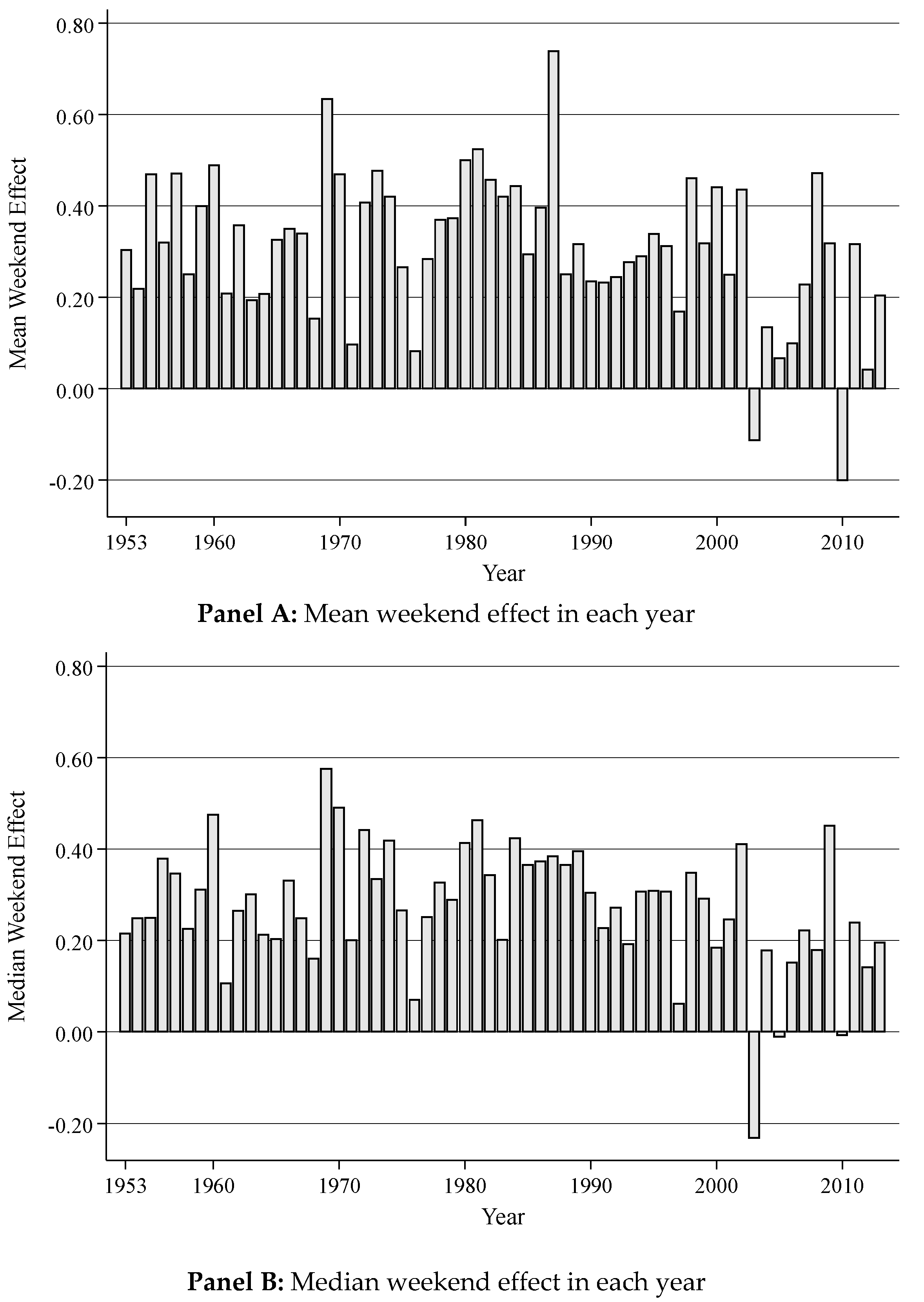
To investigate this possibility, I first calculate the weekend effect each week as the return on Friday minus the return on the following Monday, using the CRSP equal-weighted daily indices returns. Panel A of Figure 1 plots the mean weekend effect (i.e., mean of these 52 observations) in each year. Since the finding in French [2] was based on data from 1953 to 1977, an out-of-sample analysis should use only data after 1977. From 1978 to 2013, the mean weekend effect is positive in 34 out of 36 years (p-value < 0.000001 using a binomial probability test). This finding suggests that one-time events (e.g., “Black Monday of 1987”) are unlikely to cause the weekend effect.

However, because Panel A examines the mean weekend effect in each year, it is possible that the weekend effect documented is driven by some rare, but yearly recurring, events. For example, Kamstra, Kramer, and Levi [16] hypothesized a large stock price reaction in the two weekends affected by daylight savings (when clocks are adjusted in the Fall and Spring).

To rule out such possibility, Panel B plots the median weekend effect in each year (i.e., median of the 52 weekend effects in each year), and finds that the median weekend effect is positive in 33 out of the most recent 36 years (p-value < 0.000001 using a binomial probability test). While the hypothesis in Kamstra et al. [16] might explain why the mean weekend effect is significant, it is unlikely to explain why the median weekend effect is also significant (since daylight savings adjustments affects only two of the 52 weekends each year). This means that the weekend effect is unlikely to be caused by some rare, but yearly recurring, events.

4. Conclusions

Anecdotal survey suggests that most academics and practitioners currently perceive the weekend effect as an artifact of data mining, or a consequence of some unusual/rare events. My out-of-sample analysis examines–and rejects–both popular misconceptions. It also reconciles and explains how some prior studies (e.g., Schwert [14]) reached such an erroneous conclusion.

Finally, this study describes the interplay between the “weekend effect” and the “size effect”. Specifically, I find that the smallest firms have significantly higher return than the largest firms only on Thursday and Friday, but not on Monday through Wednesday. This calls into question the common practice of using “size” as a “risk factor” (unless researchers have a theory on why smaller firms are more risky on certain days of the week and earn higher returns, but are less risky and earn lower returns on other days).

References

- F. Cross. “The Behavior of Stock Prices on Fridays and Mondays.” Financ. Anal. J. 29 (1973): 67–69. [Google Scholar] [CrossRef]
- K. French. “Stock Returns and the Weekend Effect.” J. Financ. Econ. 8 (1980): 55–69. [Google Scholar] [CrossRef]
- D. Keim, and R. Stambaugh. “A Further Investigation of the Weekend Effect in Stock Returns.” J. Finance 39 (1984): 819–835. [Google Scholar] [CrossRef]
- D.B. Keim. “Trading patterns, bid-ask spreads, and estimated security returns: The case of common stocks at calendar turning points.” J. Financ. Econ. 25 (1989): 75–97. [Google Scholar] [CrossRef]
- M. Gibbons, and P. Hess. “Day of the Week Effects and Asset Returns.” J. Bus. 54 (1981): 579–596. [Google Scholar] [CrossRef]
- J. Lakonishok, and M. Levi. “Weekend Effects on Stock Returns: A Note.” J. Finance 37 (1982): 883–889. [Google Scholar] [CrossRef]
- E. Dyl, and S. Martin Jr. “Weekend Effects on Stock Returns: A Comment.” J. Finance 40 (1985): 347–349. [Google Scholar] [CrossRef]
- J. Lakonishok, and M. Levi. “Weekend Effects on Stock Returns: A Comment.” J. Finance 40 (1985): 351–352. [Google Scholar] [CrossRef]
- A. Abraham, and D. Ikenberry. “The Individual Investor and the Weekend Effect.” J. Financ. Quant. Anal. 29 (1994): 263–277. [Google Scholar] [CrossRef]
- K. Wang, Y. Li, and J. Erickson. “A New Look at the Monday Effect.” J. Finance 52 (1997): 2171–2186. [Google Scholar] [CrossRef]
- A. Damodaran. “The Weekend Effect in Information Releases: A Study of Earnings and Dividend Announcements.” Rev. Financ. Stud. 2 (1989): 607–623. [Google Scholar] [CrossRef]
- R. Thaler. “Anomalies: Seasonal Movements in Security Prices II: Weekend, Holiday, Turn of the Month, and Intraday Effects.” J. Econom. Perspect. 1 (1987): 169–177. [Google Scholar] [CrossRef]
- M. Rubinstein. “Rational Markets: Yes or No? The Affirmative Case.” Financ. Anal. J. 57 (2001): 15–29. [Google Scholar] [CrossRef]
- G.W. Schwert. “Anomalies and Market Efficiency.” In Handbook of the Economics of Finance. North Holland, The Netherlands: Elsevier, 2003. [Google Scholar]
- R. Sullivan, A. Timmermann, and H. White. “Dangers of Data-Mining: The Case of Calendar Effects in Stock Returns.” J. Econom. 105 (2001): 249–286. [Google Scholar] [CrossRef]
- M. Kamstra, L. Kramer, and M. Levi. “Losing Sleep at the Market: The Daylight Saving Anomaly.” Am. Econ. Rev. 90 (2000): 1005–1011. [Google Scholar] [CrossRef]
- R.W. Banz. “The relationship between return and market value of common stocks.” J. Financ. Econ. 9 (1981): 3–18. [Google Scholar] [CrossRef]
- J. Lakonishok, and S. Smidt. “Are seasonal anomalies real? A ninety-year perspective.” Rev. Financ. Stud. 1 (1988): 403–425. [Google Scholar] [CrossRef]
- K.L. Fisher, J. Chou, and L. Hoffmans. The Only Three Questions that Still Count: Investing by Knowing What Others Don’t. Hoboken, NJ, USA: John Wiley & Sons, 2012. [Google Scholar]
- H. Chen, and V. Singal. “Role of Speculative Short Sales in Price Formation: The Case of the Weekend Effect.” J. Finance 58 (2003): 685–706. [Google Scholar] [CrossRef]
- B.M. Blau, B.F. van Ness, and R.A. van Ness. “Short Selling and the Weekend Effect for NYSE Securities.” Financ. Manag. 38 (2009): 603–630. [Google Scholar] [CrossRef]
- H. White. “A heteroskedasticity-consistent covariance matrix estimator and a direct test for heteroskedasticity.” J. Econom. Soc. 48 (1980): 817–838. [Google Scholar] [CrossRef]
- J. Campbell, A. Lo, and A. MacKinlay. The Econometrics of Financial Markets. Princeton, NJ, USA: Princeton University Press, 1997. [Google Scholar]
- 1If expected returns on non-trading days and trading days are similar, then Monday’s return should be three times higher than Friday. Alternatively, if expected return on non-trading days (i.e., weekends) is zero, then Monday’s return should be the same as Friday.
- 2p-value < 0.000001 using a binomial probability test.
- 3Consider a volatile stock whose price rises from $1 to $2, and falls back to $1. If raw return is used (i.e., 100% and –50%, respectively), then the mean return will be spuriously positive and correlated with return volatility.
Figure 1.
Mean and median weekend effect in each year. The sample period is 1953–2013, which includes the sample periods examined in French [2] and Schwert [14], as well as the more recent years. Weekend effect is computed each week as the return on Friday minus the return on the following Monday, based on CRSP equal-weighted daily indices returns (WRDS dataset is crsp.dsi). Monday (Friday) refers to the first (last) trading day of each week. The mean and median weekend effect in each year is illustrated in Panel A and Panel B, respectively.