Are the Scaling Properties of Bull and Bear Markets Identical? Evidence from Oil and Gold Markets

Abstract

In this study, the scaling properties of the oil and gold return volatilities have been analyzed in the context of bull and bear periods. In the determination of bull and bear turning points, we used the Modified Bry-Boschan Quarterly (MBBQ) algorithm. Results showed that the business cycle phase shapes of the bear periods in the oil market are almost linear, whereas the bull and bear periods of the gold and bull period of the oil market are convex. This means that there are sharper declines in the bear period of the oil market. Following the detection of bull and bear periods, scaling exponent H analysis was performed via the aggregated variance, Higuchi’s statistic, Peng’s statistic, rescaled range, boxed periodogram and wavelet fit models, which are from the time, frequency and wavelet domains. As there are conflicts about the credibility of these methods in the literature, we have used the shuffling procedure in order to determine the most robust methods. According to the results, bear periods have higher volatility persistency than bull periods.

1. Introduction

After the studies of Benoit Mandelbrot, a great deal of interest started as concerns the fractal dimension, self-similarity and long memory features of the financial time series in the finance and econometrics literature. Despite the fact that these concepts are different from each other, scaling can be accepted as the common feature of these notions. As is stated by Barenblatt [1], if the spatial distributions of the features in different times can be obtained by similarity transformation from one another, then this time-dependent phenomenon is stated as self-similar, and it is one of the key concepts of the scaling notion. A stochastic process Y(t) can be stated as self-similar when:

$$ℒ\left(Y\left(ct\right)\right)=ℒ\left(c^{H}Y\left(t\right)\right)$$

(1)

where $ℒ$ denotes the finite joint distribution of $Y\left(t\right)$. $H$ is the self-similarity parameter, scaling exponent or scale-invariant property (Wang et al. [2]). Fractals are the best known example of the self-similarity and scale-invariant property. As stated by Kobeissis [3], a fractal is self-similar and scaled identically in all directions. Self-similarity can also exist in the probability distributions; for example, in the case that its statistical properties remain the same at all times, a probability density function is statistically self-similar. Every fractal piece presents the diminished image of the whole fractal, and they are characterized by a power law. Power law functions, which describe the probability density function of returns and autocorrelations of the volatility scales, have scale-invariant features (Segnon and Lux [4]). A general definition of the power law can be presented by Equation (2) below:

$$y\left(x\right)=x^{-n}$$

(2)

and:

$$y\left(\lambda x\right)={\lambda }^{-n}y\left(x\right)$$

(3)

In this function, the frequency of an occurrence is inversely proportional to the power (n) of its size. If we take the logarithms of both sides of the Equation (2), then we can obtain the following form:

$$\log \left(y\left(x\right)\right)=-nlog\left(x\right)$$

(4)

where n denotes the fractal dimension. The relationship, which links the self-similarity to the power law and fractal dimension, can be demonstrated by the scaling equation. For instance, for a self-similar y(t) process, a scaling relationship satisfies the following condition:

$$y\left(\lambda t\right)={\lambda }^{H}y\left(t\right)$$

(5)

where λ is a constant, H is the scaling exponent and t is a measure of the scale, which in this equation, denotes the time. It is clear that the power law obeys the scaling relationship (Komulainen [5]). One of the processes that satisfies the scaling-invariant and fractality features is the fractal Brownian motion that was first introduced by Kolmogorov [6] and presented by Mandelbrot and Van Ness [7] (Segnon and Lux [4]). For a series that follows the fractal Brownian motion: $0<H<1$. If $H=0.5$, this series is a geometric Brownian motion; if $0.5<H<1$, the series is a long memory process with persistent increments; and finally, in the case of $0<H<0.5$, the series is the short memory process. Therefore, modeling the Hurst exponent gives information about the scaling features of the time series.

Long memory and scaling properties of financial time series have been broadly discussed in the finance and econometrics literature, and as a result, a large model family has been created that also considers structural breaks and regime shifts. However, it is seen that in these studies, scaling properties of time series have been examined for the whole series. After all, many studies have demonstrated that all of the time series do not have the same statistical characteristics, and different subperiods may have different properties. For example, Pagan and Sossounov [8] and Lunde and Timmermann [9] have conducted important studies in order to determine the periods of bull and bear markets. Marcucci [10] stated that time series may consist of different regimes and showed that the Markov Regime Switching Generalized Autoregressive Conditional Heteroskedasticity model (MRS-GARCH ) outperforms the standard GARCH family models considering this reality. On the other hand, Kantelhardt et al. [11] modified the classical Detrended Fluctuations Analysis (DFA) analysis and presented the Multifractal DFA (MF-DFA) model that consider multiple scaling properties of the time series; because, it is clear that in the case of the existence of different regimes, series will have multiple scaling properties in each regime or subperiod. Under these circumstances, unlike the current literature, in this study, we analyze the scaling properties of the volatility of gold and oil markets within the context of subperiods consisted by bull and bear markets. The goal of this approach is to present the characteristics of every subperiod and to find out whether or not different periods that contain various financial or social crises affect the general behavior of the volatility of gold and oil returns. In order to reveal the idiosyncratic features of bull and bear periods, we used a long time interval consisting of the period of 20 May 1987–5 May 2014 and 1 May 1987–9 May 2014.

2. Literature Reviews

Studies about self-similarity date back to Mandelbrot [12], who is accepted as the father of fractals. In his seminal paper, Mandelbrot pointed out a new stylized fact in the financial time series, self-similarity, by exhibiting that cotton prices display the same behavior in different time scales. In the period that follows the study of Mandelbrot, a great deal of interest in self-similarity has occurred in the finance literature, and different researchers separately presented new methods for the calculation of the Hurst exponent as an alternative to Mandelbrot’ [13] rescaled range (R/S) analysis.

Geweke and Porter-Hudak [14] presented a new Hurst exponent estimator that is calculated in the frequency domain, known as the periodogram method. In fact, even though this estimator is the fractional difference operator, it can be transformed to the Hurst exponent by the equation $d=H-0.5$. Another study about the calculation of the Hurst exponent H was conducted by Higuchi [15]. Higuchi provided a model to measure the fractal dimension of the set of points (t, f(t)) forming the graph of a function f defined on the unit interval and gave evidence, performing his model using two different data; one of them has a scaling property, and the other does not. Using daily and monthly data, Lo [16] has shown that when short memory is taken into account, R/S analysis fails, and that is why he proposed to modify R/S analysis, so that it is robust to the short memory. Using the long memory and short memory series, Peng et al. [17] analyzed the issue of whether long memory features arise from the mosaic structure of DNA or not. They used a fluctuation analysis in order to distinguish the properties of these two different data. Taqqu et al. [18] proposed variance type models for the calculation of the Hurst exponent. Teverovsky and Taqqu [19] examined the performances of different models via the fractional Gaussian noise and the Fractional Autoregressive Integrated Moving Average (ARFIMA) (0.d.0) simulations. Abry and Veitch [20] developed a wavelet-based estimator for the estimation of the Hurst exponent. According to the results, this estimator gave efficient results under a normal distribution and very general conditions. As was stated by the authors, their model was quite robust, even with the conditions that there were deterministic trends in the series. Audit et al. [21] analyzed different wavelet-based estimators, and as a conclusion, they showed that the wavelet transform modulus maxima (WTMM) gives the best results on the basis of mean square error. Recently, Simonsen et al. [22] proposed a new wavelet-based estimator. According to their results, when one or only a few samples are available, the wavelet method outperforms the Fourier method. In another recent study, Liu et al. [23] presented a new estimator that is based on the refined form of the spectral density function. They also showed the robustness of this estimator against the wavelet maximum likelihood model via Monte Carlo simulations.

The aforementioned studies, which can be classified in the context of the time, frequency and wavelet domain, examine the scaling exponent H in the monofractal basis. However, Mandelbrot [24], Mandelbrot et al. [25] and Mandelbrot et al. [26] proposed multiscaling, that is the multifractal concept. In one of these studies, Mandelbrot et al. [25] exhibited the multifractal model of asset returns model as an alternative to the Autoregressive Conditional Heteroskedasticity (ARCH) type models. Kantelhardt et al. [11] presented the MF-DFA model improving the mono-scaling model of Peng et al. [17] via the multiscaling approach. As for Calvet and Fisher [27], they proposed the discrete-time stochastic volatility model in the modeling of multifractal processes.

In the business cycles literature, the first robust algorithm about the turning points was presented by Bry and Boschan [28]. Afterwards, this model was modified by Pagan and Sossounov [8] in order to apply it to a monthly time series. Likewise, Harding and Pagan [29] built the Bry-Boschan Quarterly (BBQ) model, which is based on the Bry and Boschan [28] algorithm. In the following years, many models have been improved by different researchers in order to analyze the business cycle phases of the financial and economic time series. In one of these studies, Lunde and Timmermann [9] used a cumulative return threshold for the establishment of turning points. More recently, Maheu et al. [30] presented a new Markov switching model for the determination of bull and bear market regimes in stock returns. They stated that their model fully describes the return distribution while, treating business cycles as unobservable. As an alternative, Engle [31] presented the Modified Bry-Boschan Quarterly (MBBQ) algorithm modifying the model of Harding–Pagan. Subsequently, in many studies, this algorithm has been used in order to determine the bull and bear periods or turning points. In one of these studies, Abbritti and Fahr [32] analyzed the effects of the degree of downward wage rigidities to the other variables in the economy. Tsouma [33] examined whether or not the Greek economy entered recession during the period of mortgage crisis via the MBBQ algorithm and concluded that Greece could not overcome the recession still in 2010. Einarsson et al. [34] investigated the structure of Icelandic business cycles and showed that the business cycle of Iceland is to a large extent asymmetric to the business cycle of other developed countries. In a different study, Aastveit et al. [35] determined four recessions via the MBBQ algorithm during the period of 1978Q1 to 2011Q4 in the GDP of the Norwegian mainland. More recently, Ingram [36] analyzed the cycles of commodity prices via the MBBQ algorithm and obtained similar results for different commodities. According to the findings, when the commodity prices rise, the highest risings are observed in the last period. Similarly, the largest falls occur in the last period of the market crash.

Following the literature reviews, the rest of the paper is organized as follows: In Section 3, we present the theoretical framework of the models that are used in the empirical analysis. In Section 4, we examine the findings of statistical tests of the scaling analysis of gold and oil volatilities after the identification of bull and bear periods. Finally, Section 5 discuss the results of the overall analysis.

3. Econometrical Methodology

In this study, in order to analyze the scaling behaviors of the oil and gold volatilities, we used different methods from the time, frequency and wavelet domains. This section gives theoretical information about the MBBQ algorithm and scaling exponent H estimators.

As stated before, in the analyzing of the scaling properties of oil and gold market volatilities, we use different methods, such as: aggregated variance, Higuchi’s statistic, Peng’s statistic, rescaled range, boxed periodogram and wavelet fit models. According to the existing literature, there is not a consensus about the performance of these models. It is hoped that our findings will be beneficial to this argument. Some of the recent studies revealed that R/S analysis underperforms compared to other alternative models. For example, Witt and Malamud [37] suggest not to use R/S analysis because of the large systematic errors of the model. They also stated that Peng’s statistic displays successful performance when the tail of the probability density function is thin. Similarly, Rea et al. [38] stated that R/S analysis has some problems: the model displays upward biases when H is low and otherwise shows downward biases. In addition, they showed that boxed periodogram and Higuchi’s statistic were also biased towards underestimating H values. Ye et al. [39] showed that in the case of the long memory process displaying linear trends, the wavelet statistic presents unbiased results. Likewise, Jeonga et al. [40] demonstrated that wavelet statistic and Whittle maximum likelihood estimators have the lowest biases.

3.1. MBBQ Algorithm

James Engle presented the MBBQ algorithm by modifying Harding and Pagan’s [29] BBQ algorithm, which was based on the Bry and Boschan [28] study. Let ${\wedge }_t=1 \text{and} {\vee }_t=1$ denote peaks and troughs at time t, respectively. In this case, peaks and troughs can be stated as follows:

$${\wedge }_{t }=1\left\{\left(y_{t-k},\dots ,y_{t-1}\right)<y_t>\left(y_{t+1},\dots ,y_{t+k}\right)\right\}$$

(6)

where y_t is the unobserved series. Regarding alternate phases, if S_t indicates the business cycle, it takes a value of one in expansions and zero in contractions. Equation (7) below indicates the minimum phase duration of the recursion for monthly data:

$$S_t=S_{t-1}\left(1-S_{t-2}\right)+S_{t-1}{S}_{t-2}\left(1-S_{t-3}\right)+S_{t-1}{S}_{t-2}{S}_{t-3}\left(1-S_{t-4}\right)$$

(7)

The first two lines in the above equation establish that the expansions have a minimum period of five months. The third line permits the continued expansion to exceed the five-month period, provided that we do not come across a peak. If we do come across a peak, the phase is switched to a contraction. The fourth line removes the contractions of more than a five-month duration resulting from detecting a trough. For further reading, see Harding [41].

3.2. Aggregated Variance Method

Using the process stated by Sun et al. [42], we can demonstrate the calculation of the scaling exponent H via the aggregated variance method as follows: A time series of length N is divided into subgroups of length m. The mean of the each subgroup can be calculated as below:

$${\stackrel{-}{X}}_k^{\left(m\right)}:=\frac{1}{\text{m}}{\displaystyle \sum }_{t=\left(k-1\right)m+1}^{km}{X}_t$$

(8)

variance:

$${\stackrel{-}{\sigma }}_m^2:=\frac{1}{\left[\frac{N}{m}\right]-1}{\displaystyle \sum }_{k=1}^{\left[\frac{N}{m}\right]}{\left({\stackrel{-}{X}}_k^{\left(m\right)}-\stackrel{-}{X}\right)}^2$$

(9)

The slope of the plot of $log{\stackrel{-}{\sigma }}_m^2$ versus logm provides the calculation of the scaling exponent H. If the slope of this plot is −1, this means that scaling exponent $H=0.5$ and demonstrates that there is no long memory or resistance in the series.

3.3. Higuchi’s Statistic

In this method, first, the partial sums of the time series $X_i, i=1,\mathrm{...},N$, are calculated: $Y\left(n\right)={\displaystyle \sum }_{i=1}^n{X}_i$. Afterwards, the normalized line of the curve is found as follows:

$$L\left(m\right)=\frac{N-1}{m^3}{\displaystyle \sum }_{i=1}^m{\left[\frac{N-i}{m}\right]}^{-1}{\displaystyle \sum }_{k=1}^{\left[\frac{N-i}{m}\right]}\left|Y\left(i+km\right)-Y\left(i+\left(k-1\right)m\right)\right|$$

(10)

where N is the length of the series, m is the block size and $[]$ demonstrates the highest integer function. The slope of the $L\left(m\right)$ in the log-log plot versus m gives d. Using the equation $d=2-H$, we can obtain the scaling exponent H (Taqqu et al. [18]).

3.4. Rescaled Range Analysis (R/S)

Following the explanation of Lo [16], we can calculate the scaling exponent H as below:

$$H=\frac{1}{{\sigma }_n}\left[\underset{1\le k\le n}{\text{Max}}{\displaystyle \sum }_{j=1}^k\left(r_j-{\stackrel{-}{r}}_n\right)-\underset{1\le k\le n}{\text{Min}}{\displaystyle \sum }_{j=1}^k\left(r_j-{\stackrel{-}{r}}_n\right)\right]$$

(11)

where r₁,r₂,..., r_n are the returns of the time series and ${\stackrel{-}{r}}_n$ is the mean of the returns. As for σ_n, it denotes the maximum likelihood estimator of the standard deviation.

3.5. Peng’s Statistic

Let x_k be a time series of length N. First, we build the profile as follows: $Y\left(i\right)\equiv {\displaystyle \sum }_{k=1}^i\left[x_k-\stackrel{-}{x}\right]$. Splitting the $Y\left(i\right)$ into subdivisions ($v$) of equal length s from beginning to end and end to beginning, we obtain $N_s$ number divisions and fit local trends for every subdivision with OLS. Afterwards, we remove the local trends and calculate the variance for every subdivision:

$$F^2\left(v,s\right)\equiv \frac{1}{s}{\displaystyle \sum }_{i=1}^s{\left\{Y\left[\left(v-1\right)s+i\right]-y_v\left(i\right)\right\}}^2$$

(12)

The variance of the detrended profile for every subdivision provides the mean-square fluctuation:

$$F_{DFAm}^2\left(v,s\right)=\frac{1}{s}{\displaystyle \sum }_{i=1}^s{\tilde{Y}}_s^2\left(i\right)$$

(13)

In the next step, we obtain mean fluctuations by calculating the means for all of the subdivisions: $F_2\left(s\right)$. The scaling relationship $F_2\left(s\right)~s^{\alpha }$ exhibits the scaling exponent, $\alpha =H$ (Kantelhardt [43]).

3.6. Boxed Periodogram Method

The periodogram method gives a plot of the logarithms of the spectral density of the time series that is studied on the logarithm of frequencies. The slope of this plot provides the estimation of the scaling exponent H. The periodogram can be stated as below:

$$I\left(\lambda \right)=\frac{1}{2\pi T}{\left|{\displaystyle \sum }_{j=1}^{N}x\left(j\right)e^{ij\lambda }\right|}^2$$

(14)

where x is the time series, T is the length of the time series and λ is the frequency (Goergen and Viala [44]). In the boxed periodogram method, the frequency axis is divided into equal boxes, and the mean of the periodogram values concerning the frequencies within boxes are calculated (Paxson et al. [45]).

3.7. Wavelet Statistic

Abry and Veitch [20] presented a wavelet-based Hurst estimator. Let j₁ and j₂ denote the scales; in this case, the weighted least square fit between these two scales exhibits the Hurst exponent formula as follows:

$$H\left(j_1,j_2\right)\equiv \frac{1}{2}\left[\frac{{{\displaystyle \sum }}_{j=j_1}^{j_2}{S}_{j}j{\eta }_j-{{\displaystyle \sum }}_{j=j_1}^{j_2}{S}_{j}j{{\displaystyle \sum }}_{j=j_1}^{j_2}{S}_j{\eta }_j}{{{\displaystyle \sum }}_{j=j_1}^{j_2}{S}_j{{\displaystyle \sum }}_{j=j_1}^{j_2}{S}_j{j}^2-{({{\displaystyle \sum }}_{j=j_1}^{j_2}{S}_{j}j)}^2}+1\right]$$

(15)

where ${\eta }_j=lo{g}_2\left(\frac{1}{n_j}{\displaystyle \sum }_k{\left|d_x\left(j,k\right)\right|}^2\right)$ and weight $S_j=\frac{n{\text{ln}}^{2}2}{2^{j+1}}$ is the inverse of the theoretical asymptotic variance of η_j.

4. Empirical Analysis and Data

In this study, we analyzed the scaling properties of the volatilities of the oil and gold returns concerning bull and bear markets. Oil data is the daily Brent crude oil absolute returns, and gold is the daily troy ounce absolute returns. The period of the data consisting of the oil and gold series is 20 May 1987–5 May 2014 and 1 May 1987–9 May 2014, respectively. Although the scaling analysis has been conducted with daily data, in order to determine turning points for the bull and bear markets, we have used monthly price data for both of the series due to the necessity of the MBBQ algorithm.

4.1. Determination of Bull and Bear Periods

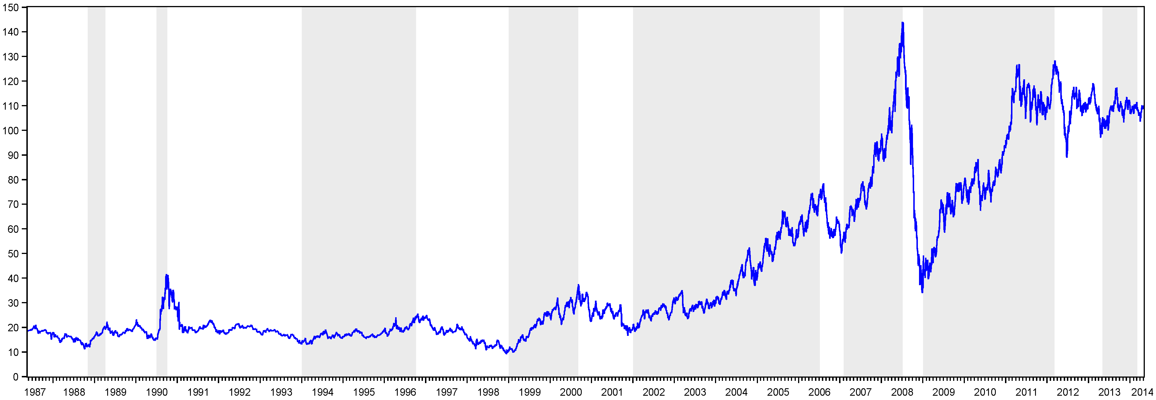
Table 1 presents the peak and trough dates obtained via the MBBQ algorithm in the oil and gold markets. For the oil and gold data, we have determined seven peaks/eight troughs and five peaks/five troughs, respectively. In addition to this information, as can be seen from Figure 1, the oil market has eight bull and nine bear periods, whereas the gold market has six bear and five bull periods. Due to its very short duration, we leave the last bear period out of the assessment in the oil data. Therefore, in the following sections of the paper, we will use eight bear and eight bull periods for the oil market.

Table 1. Peak and trough dates of the oil and gold markets.

OIL		GOLD
Peaks	Troughs	Peaks	Troughs
03.01.1989	09.01.1988	10.31.1991	05.31.1990
09.01.1990	05.01.1990	06.30.1993	01.29.1993
09.01.1996	11.01.1993	12.29.1995	12.30.1994
08.01.2000	11.01.1998	01.31.2008	07.30.1999
06.01.2006	11.01.2001	07.29.2011	09.30.2008
06.01.2008	12.01.2006	-	-
02.01.2012	11.01.2008	-	-
-	03.01.2013	-	-

Table 1. Peak and trough dates of the oil and gold markets.

OIL		GOLD
Peaks	Troughs	Peaks	Troughs
03.01.1989	09.01.1988	10.31.1991	05.31.1990
09.01.1990	05.01.1990	06.30.1993	01.29.1993
09.01.1996	11.01.1993	12.29.1995	12.30.1994
08.01.2000	11.01.1998	01.31.2008	07.30.1999
06.01.2006	11.01.2001	07.29.2011	09.30.2008
06.01.2008	12.01.2006	-	-
02.01.2012	11.01.2008	-	-
-	03.01.2013	-	-

Figure 1. Bull and bear periods of the oil market.

Figure 1. Bull and bear periods of the oil market.

As can be seen from Figure 1, the longest bear market period in oil price is between the last quarter of 1990 and 1994, whereas the longest bull market is between 2002 and the first half of 2006. On the other hand, the period between the second half of 2008 and 2009 is the strongest bear market. However, it is seen that this drop recovered in six months, similar to black Monday in 1987.

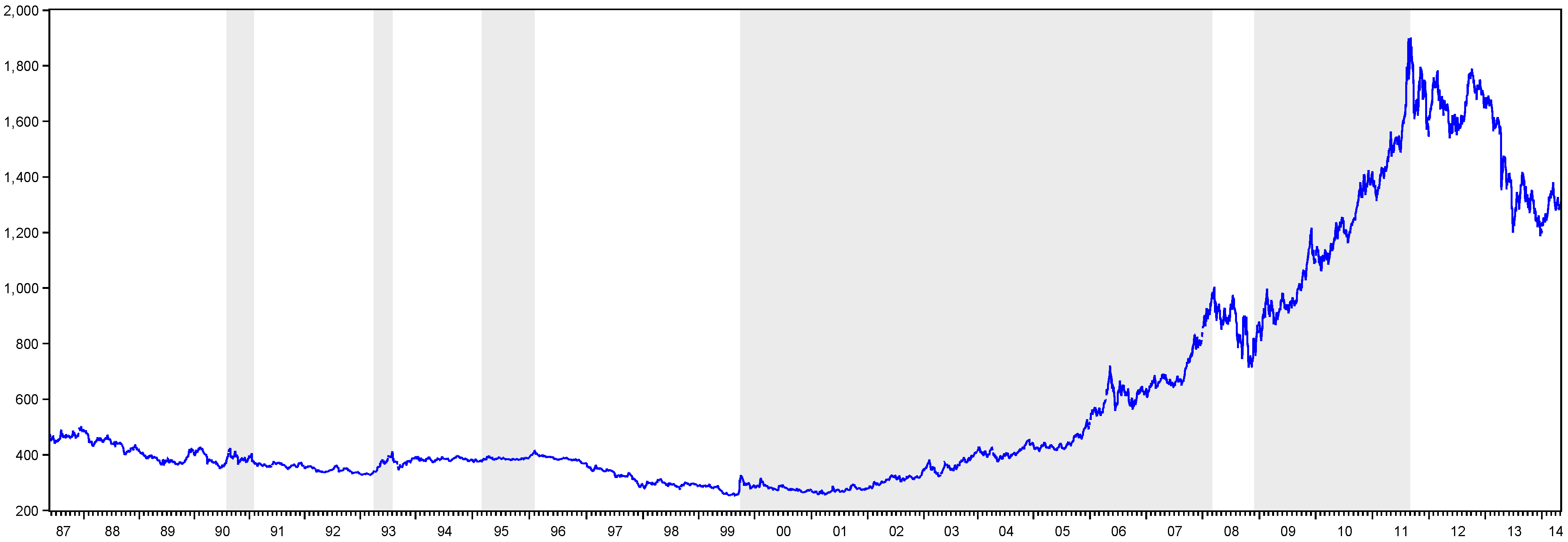
In the gold market, Figure 2 exhibits that the longest bear periods are seen between the second half of 1987 and the first half 1990 and also between 1996 and the last quarter of 1999. In addition, there is a long bull period between the last quarter of 1999 and the first quarter of 2008. On the other hand, we have seen that while its slope is not as sharp as the oil market, there is a drastic fall in the period of the mortgage crises, which recovered in nine months.

Figure 2. Bull and bear periods of the gold market.

Figure 2. Bull and bear periods of the gold market.

In order to characterize the bull and bear periods better, we have presented in Table 2 three statistics: duration (D), amplitude (A) and excess (E), described by Harding and Pagan [29]. One of these statistics, duration, demonstrates the mean duration of every phase (C). The second statistic, amplitude, gives the magnitude of the log price difference of any asset from one turning point to another. As for excess, it is the mean of overall phases, and it exhibits an index value for the shape of the phases. As stated by Camacho et al. [46], the excess statistic measures the deviations of the time series from the hypothetical linear path that is described by the model. The duration, amplitude and excess can be commented on as the features of business cycles: length, depth and shape, respectively.

Table 2. Harding and Pagan’s bull and bear market statistics.

	OIL		GOLD
	Bears	Bulls	Bears	Bulls
Duration	16.7143 (0.6975)	25.2857 (0.7298)	21 (0.7264)	34 (1.1615)
Amplitude	−0.6364 (−0.6099)	0.9377 (0.3510)	−0.2417 (−0.7090)	0.5181 (1.1196)
Excess 1	−0.9683 (−21.7465)	6.7198 (2.2837)	12.1319 (3.2496)	9.2775 (7.0006)

Table 2. Harding and Pagan’s bull and bear market statistics.

	OIL		GOLD
	Bears	Bulls	Bears	Bulls
Duration	16.7143 (0.6975)	25.2857 (0.7298)	21 (0.7264)	34 (1.1615)
Amplitude	−0.6364 (−0.6099)	0.9377 (0.3510)	−0.2417 (−0.7090)	0.5181 (1.1196)
Excess 1	−0.9683 (−21.7465)	6.7198 (2.2837)	12.1319 (3.2496)	9.2775 (7.0006)

As can be seen from the results of Table 2, the mean duration of the bull period is longer than the bear period in both the oil and gold markets. On the other hand, both durations in the gold market are longer than the oil market. Results obtained for the oil market correspond to the findings of Pagan and Sossounov [8]. They analyzed the stock prices of the U.S. for three different periods, January 1835–May 1997, January 1889–May 1997 and January 1945– May 1997, and showed that the bull-bear durations are 25–15, 25–14 and 27–12, respectively.

The findings of the gold market are quite different from the oil market. The duration of its bull and bear periods is longer than the oil market’s results. This situation can be explained by the gold market being more stable than the oil market. Using the excess statistics, we can comment about the shape of the business cycle phases. For instance, close to zero, but negative excess value, −0.9683, of the bear periods in the oil market means that this phase is approximately linear and slightly concave. Conversely, the positive excess value, 12.1319, of the bear periods of the gold market indicates that the phase has a convex shape. These results are also valid for the bull periods in the gold market. The positive values in the oil and gold market indicate that here, the phases have a convex structure, that is the bull period is formed by a smooth growth rate in the beginning, but in the last part of the expansion, there are sharp movements. As a conclusion, we can say that small excess values in the oil market means that there are sharper movements in the bull and bear periods than the gold market.

4.2. Scaling Analysis of the Oil and Gold Return Volatilities

In this section of the study, we perform the scaling analysis for the volatilities of the oil and gold returns. The scaling analysis has been conducted for the bull and bear periods separately, and we have used the time, frequency and wavelet domains in the calculation of the scaling exponent H. The methods that we have used can be classified as follows: the aggregated variance, Higuchi’s statistic, Peng’s statistic and rescaled range methods are in the time domain; the boxed periodogram is in the frequency domain; and finally, the wavelet fit method is in the wavelet domain.

4.2.1. Scaling Analysis of the Oil Return Volatility in the Bull and Bear Periods

Before we separated the oil return volatility for different bull and bear periods, we first examined the scaling property of the whole series under all of the methods and presented the findings in Table 3. As stated by Teverovsky et al. [47], because there are difficulties in performing the modified R/S analysis of Lo [16], we left the modified R/S analysis out of the context of this study. According to the results, oil return volatilities have scaling persistency features for all of the methods that we have used. According to the results of Table 3, the Higuchi’s statistic has the highest H value, whereas the lowest scaling exponent H value belongs to the R/S method. As is seen, all of the methods exhibit a scaling exponent value that is in a wide range and has a persistency property in the volatility.

Table 3. Scaling exponent H test results of oil return volatilities (full period).

	Aggregated Variance	Higuchi’s Statistic	Peng’s Statistic	R/S Statistic	Boxed Periodogram	Wavelet Fit
Original Oil_abs Series	0.8298 ** (0.0377) 0.0000	0.9725 ** (0.0299) 0.0000	0.7073 ** (0.0526) 0.0000	0.7930 ** (0.0191) 0.0000	0.6626 ** (0.0317) 0.0000	0.7819 ** (0.0345) 0.0000

** indicates the 95% and 99% confidence level.

Table 3. Scaling exponent H test results of oil return volatilities (full period).

	Aggregated Variance	Higuchi’s Statistic	Peng’s Statistic	R/S Statistic	Boxed Periodogram	Wavelet Fit
Original Oil_abs Series	0.8298 ** (0.0377) 0.0000	0.9725 ** (0.0299) 0.0000	0.7073 ** (0.0526) 0.0000	0.7930 ** (0.0191) 0.0000	0.6626 ** (0.0317) 0.0000	0.7819 ** (0.0345) 0.0000

** indicates the 95% and 99% confidence level.

In this stage, we analyze the robustness of the results via the shuffling method. The shuffling method gives a randomly shuffled series and, therefore, removes all of the correlations in the series. Hence, theoretically, we expect that there will not be persistent volatility in the shuffled series, that is the new scaling exponent H values will be close to 0.5, which demonstrates the random walk behaviors. In this situation, any large deviations from the 0.5 value means that the related method is not robust, and its results are spurious. As stated by Lina et al. [48], the shuffling procedure randomizes the order of returns of original series and breaks the memory structure of series. Therefore, the power law behavior of the scaling function displays random walk properties. On the other hand, we can save the mean and variance of the series in the shuffling process, and as the frequency properties are not changed, the probability density function of the series remains the same.

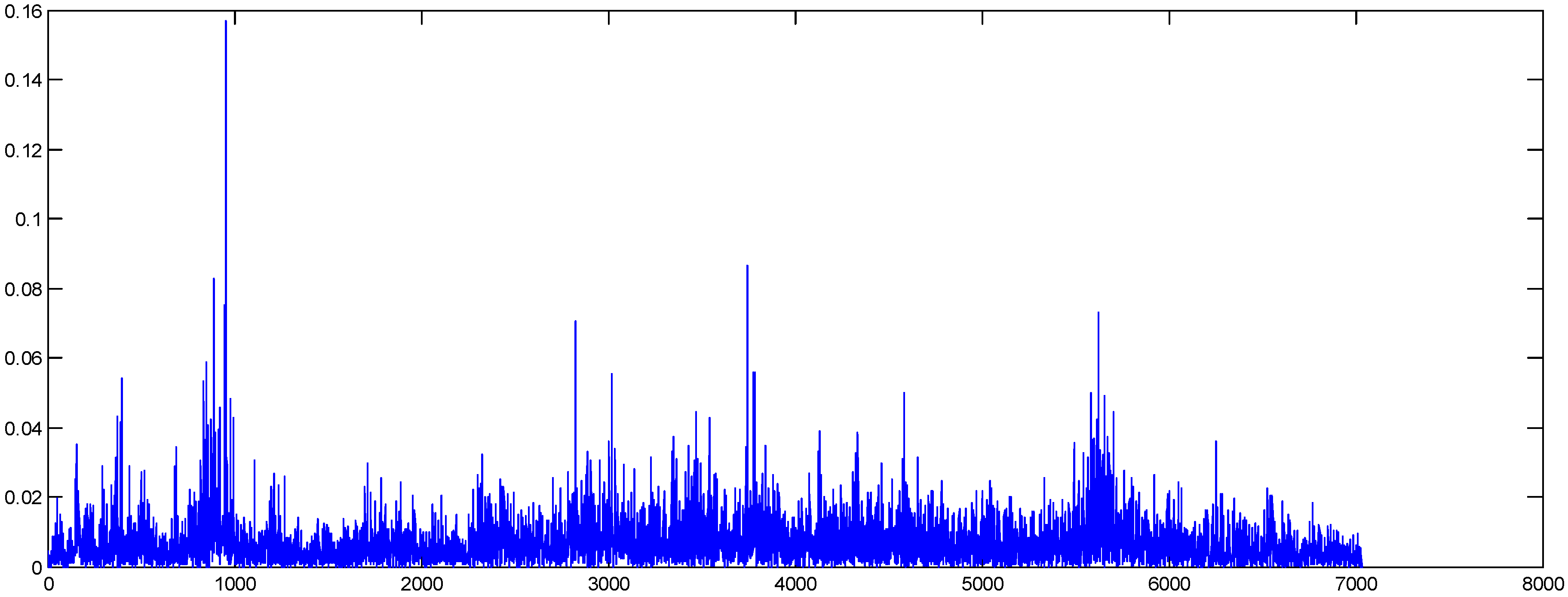
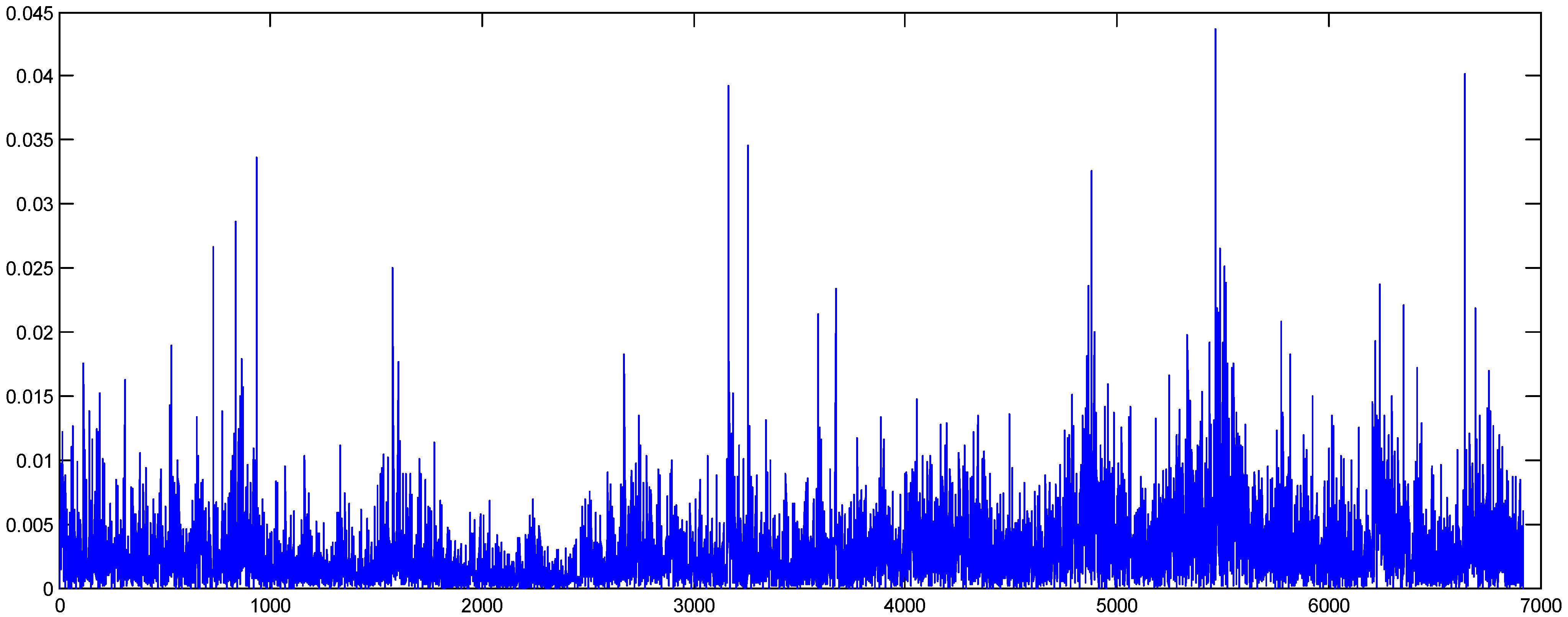
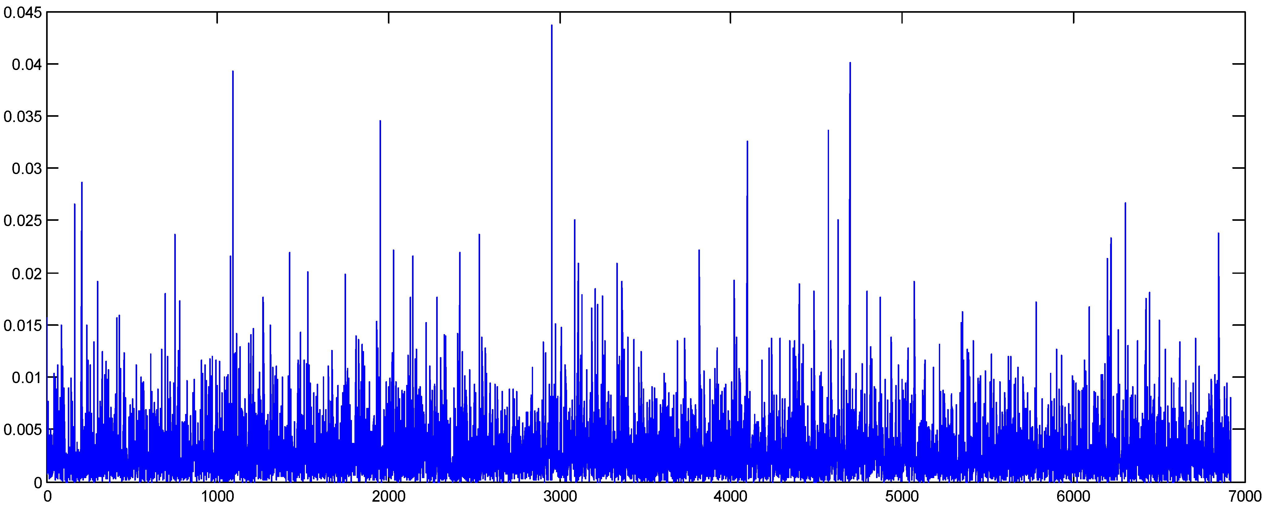
In Figure 3 and Figure 4, we present the original and shuffled series of the oil absolute returns. As can be seen, the volatility clustering of the series has been removed by the shuffling method.

Figure 3. Oil absolute returns (original data).

Figure 3. Oil absolute returns (original data).

Figure 4. Oil absolute returns (shuffled data).

Figure 4. Oil absolute returns (shuffled data).

The results of the scaling exponent H of the shuffled data are presented in Table 4. Although the correlations of the absolute returns have been destroyed by the shuffling procedure, we see that there are still findings related to persistency in some results. For instance, the Higuchi’s statistic result is almost the same as its previous value; the method still demonstrates high persistency in the volatility, even after the shuffling operation. On the other hand, unlike the findings of Cano and Manzoni [49], we see that the results of the aggregated variance method are quite robust, whereas the credibility of the R/S analysis is not explicit.

Table 4. Robustness analysis of the scaling exponent H models.

	Aggregated Variance	Higuchi’s Statistic	Peng’s Statistic	R/S Statistic	Boxed Periodogram	Wavelet Fit
Shuffled Oil_abs Series	0.5146 ** (0.0199) 0.0000	0.9660 ** (0.0284) 0.0000	0.5024 ** (0.0104) 0.0000	0.5813 ** (0.0343) 0.0000	0.4475 ** (0.0294) 0.0000	0.5216 ** (0.0115) 0.0000

** indicates the 95% and 99% confidence level.

Table 4. Robustness analysis of the scaling exponent H models.

	Aggregated Variance	Higuchi’s Statistic	Peng’s Statistic	R/S Statistic	Boxed Periodogram	Wavelet Fit
Shuffled Oil_abs Series	0.5146 ** (0.0199) 0.0000	0.9660 ** (0.0284) 0.0000	0.5024 ** (0.0104) 0.0000	0.5813 ** (0.0343) 0.0000	0.4475 ** (0.0294) 0.0000	0.5216 ** (0.0115) 0.0000

** indicates the 95% and 99% confidence level.

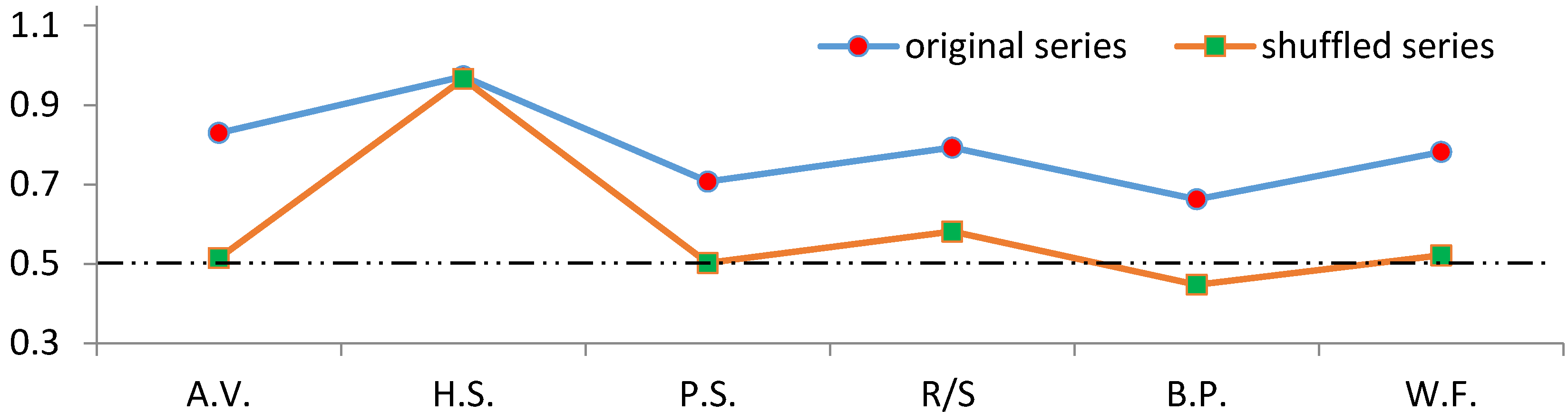
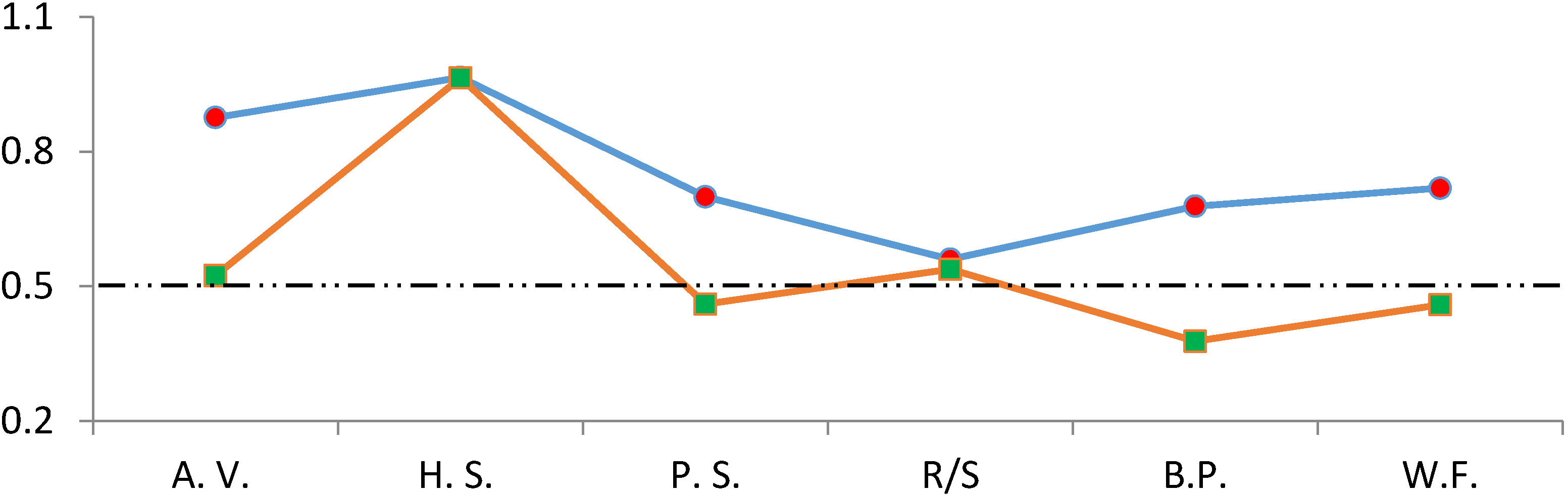
In order to efficiently comment on the results, we have presented the scaling exponent H results of both the original and shuffled series in the same graph in Figure 5. The graph indicates that every model’s scaling exponent H value, except for Higuchi’s statistic, has explicitly decreased after the shuffling operation. The closest values to 0.50 were obtained by the aggregated variance, Peng’s statistic and wavelet fit methods. Consequently, in this stage, it is clear that the most credible methods are these three models.

Figure 5. Original and shuffled series’ scaling exponent test results.2

Figure 5. Original and shuffled series’ scaling exponent test results.2

After the establishment of the credibility of the scaling exponent methods, we analyze the scaling behaviors of the return volatility of the bull and bear markets separately and exhibit the differences between the periods depending on its existence. In the following section, first, we present the scaling exponent test results of the oil return volatility for the bull and bear markets. As is stated above, we identified nine bull and eight bear periods in the oil price series using the MBBQ algorithm. As the last bull market’s duration was quite short, we did not take this period into account in the scaling analysis. Therefore, we examined the eight bull and eight bear periods for the oil market.

In the comparison of the bull and bear markets’ performances, concerning the data interval, we matched the first bull or bear period with the following phase. As is seen from Figure 1, the first phase in the oil market is the bear period; hence, we compared the first bear period with the first bull period, and we implemented the same principle for the following periods. Table 5 demonstrates that, except for the seventh bull and bear periods, all of the bear phases have higher scaling exponent H values, that is self-similarity and persistency features are much greater in the bear periods. These results also coincide with the findings of Gursakal [50]. She shows that the stock return persistency in the Turkish stock market is higher in the bear periods than the bull periods. Another important result of our analysis is that the volatility persistency of the bull market starts to get higher following the fifth period. It is beneficial to note that the volatility persistence in the seventh bull market, which corresponds to the mortgage crisis, is much higher than the previous bull market, meaning that there is a positive recovering period after the mortgage crisis.

Table 5. Scaling exponent H results of the bull and bear periods of the oil data.

PANEL A	BEARS 1	BEARS 2	BEARS 3	BEARS 4	BEARS 5	BEARS 6	BEARS 7	BEARS 8
Aggregated Variance	0.6807 ** (0.0271) 0.0000	0.7107 ** (0.0249) 0.0000	0.8862 ** (0.0161) 0.0000	0.7619 ** (0.0226) 0.0000	0.6121 ** (0.0306) 0.0000	0.5382 ** (0.0427) 0.0000	0.8370 ** (0.0753) 0.0016	0.7720 ** (0.0206) 0.0000
Peng’s Statistic	0.7802 ** (0.0194) 0.0000	0.7725 ** (0.0240) 0.0000	0.8098 ** (0.0342) 0.0000	0.5763 ** (0.0147) 0.0000	0.6533 ** (0.0163) 0.0000	0.5218 ** (0.0233) 0.0000	0.4607 ** (0.0322) 0.0000	0.6915 ** (0.01942) 0.0000
Wavelet Fit	0.8597 * (0.0974) 0.0126	0.5661 * (0.0882) 0.0234	0.8673 * (0.1938) 0.0208	0.5838 * (0.1458) 0.0279	0.3886 * (0.0893) 0.0490	0.4934 (0.2030) 0.2485	0.1849 (0.1523) 0.4386	0.6568 (0.1843) 0.0705
PANEL B	BULLS 1	BULLS 2	BULLS 3	BULLS 4	BULLS 5	BULLS 6	BULLS 7	BULLS 8
Aggregated Variance	0.5620 ** (0.0503) 0.0000	0.7980 ** (0.2077) 0.0003	0.7040 ** (0.0186) 0.0000	0.6759 ** (0.0233) 0.0000	0.4475 ** (0.0436) 0.0000	0.3302 ** (0.0242) 0.0000	0.8916 ** (0.0227) 0.0000	0.6977 ** (0.0369) 0.0000
Peng’s Statistic	0.6695 ** (0.0603) 0.0000	0.5533 ** (0.0944) 0.0000	0.6243 ** (0.0210) 0.0000	0.5366 ** (0.0125) 0.0000	0.6311 ** (0.0130) 0.0000	0.5304 ** (0.0149) 0.0000	0.7315 ** (0.0245) 0.0000	0.5160 ** (0.0226) 0.0000
Wavelet Fit	0.4977 (0.2109) 0.2551	0.4519 (0.4753) 0.5160	0.6690 ** (0.0559) 0.0002	0.5144 ** (0.0709) 0.0053	0.6685 ** (0.0617) 0.0004	0.4897 (0.1736) 0.1060	0.6258 * (0.1281) 0.0164	0.5332 ** (0.0530) 0.0097

* and ** indicate the 95% and 99% confidence level.

Table 5. Scaling exponent H results of the bull and bear periods of the oil data.

PANEL A	BEARS 1	BEARS 2	BEARS 3	BEARS 4	BEARS 5	BEARS 6	BEARS 7	BEARS 8
Aggregated Variance	0.6807 ** (0.0271) 0.0000	0.7107 ** (0.0249) 0.0000	0.8862 ** (0.0161) 0.0000	0.7619 ** (0.0226) 0.0000	0.6121 ** (0.0306) 0.0000	0.5382 ** (0.0427) 0.0000	0.8370 ** (0.0753) 0.0016	0.7720 ** (0.0206) 0.0000
Peng’s Statistic	0.7802 ** (0.0194) 0.0000	0.7725 ** (0.0240) 0.0000	0.8098 ** (0.0342) 0.0000	0.5763 ** (0.0147) 0.0000	0.6533 ** (0.0163) 0.0000	0.5218 ** (0.0233) 0.0000	0.4607 ** (0.0322) 0.0000	0.6915 ** (0.01942) 0.0000
Wavelet Fit	0.8597 * (0.0974) 0.0126	0.5661 * (0.0882) 0.0234	0.8673 * (0.1938) 0.0208	0.5838 * (0.1458) 0.0279	0.3886 * (0.0893) 0.0490	0.4934 (0.2030) 0.2485	0.1849 (0.1523) 0.4386	0.6568 (0.1843) 0.0705
PANEL B	BULLS 1	BULLS 2	BULLS 3	BULLS 4	BULLS 5	BULLS 6	BULLS 7	BULLS 8
Aggregated Variance	0.5620 ** (0.0503) 0.0000	0.7980 ** (0.2077) 0.0003	0.7040 ** (0.0186) 0.0000	0.6759 ** (0.0233) 0.0000	0.4475 ** (0.0436) 0.0000	0.3302 ** (0.0242) 0.0000	0.8916 ** (0.0227) 0.0000	0.6977 ** (0.0369) 0.0000
Peng’s Statistic	0.6695 ** (0.0603) 0.0000	0.5533 ** (0.0944) 0.0000	0.6243 ** (0.0210) 0.0000	0.5366 ** (0.0125) 0.0000	0.6311 ** (0.0130) 0.0000	0.5304 ** (0.0149) 0.0000	0.7315 ** (0.0245) 0.0000	0.5160 ** (0.0226) 0.0000
Wavelet Fit	0.4977 (0.2109) 0.2551	0.4519 (0.4753) 0.5160	0.6690 ** (0.0559) 0.0002	0.5144 ** (0.0709) 0.0053	0.6685 ** (0.0617) 0.0004	0.4897 (0.1736) 0.1060	0.6258 * (0.1281) 0.0164	0.5332 ** (0.0530) 0.0097

* and ** indicate the 95% and 99% confidence level.

4.2.2. Scaling Analysis of the Gold Return Volatility in the Bull and Bear Periods

Similar to the analysis conducted for the oil market, before the examination of the scaling properties of the bull and bear periods for the gold market, we performed the scaling exponent analysis using all of the methods for whole data of the gold absolute return series. As can be seen from the results in Table 6, all of the H values are statistically significant at a 99% confidence level, that is the scaling property of the series exhibits persistency in the volatility. The lowest H value (0.5604) belongs to the R/S analysis, whereas Higuchi’s statistic has the highest scaling exponent H value (0.9654) between different methods.

Table 6. Scaling exponent H test results of gold return volatilities (full period).

	Aggregated Variance	Higuchi’s Statistic	Peng’s Statistic	R/S Statistic	Boxed Periodogram	Wavelet Fit
Original Gold_abs Series	0.8758 ** (0.0218) 0.0000	0.9654 ** (0.0284) 0.0000	0.6995 ** (0.0490) 0.0000	0.5604 ** (0.0603) 0.0000	0.6784 ** (0.0293) 0.0000	0.7187 ** (0.0344) 0.0000

** indicates the 95% and 99% confidence level.

Table 6. Scaling exponent H test results of gold return volatilities (full period).

	Aggregated Variance	Higuchi’s Statistic	Peng’s Statistic	R/S Statistic	Boxed Periodogram	Wavelet Fit
Original Gold_abs Series	0.8758 ** (0.0218) 0.0000	0.9654 ** (0.0284) 0.0000	0.6995 ** (0.0490) 0.0000	0.5604 ** (0.0603) 0.0000	0.6784 ** (0.0293) 0.0000	0.7187 ** (0.0344) 0.0000

** indicates the 95% and 99% confidence level.

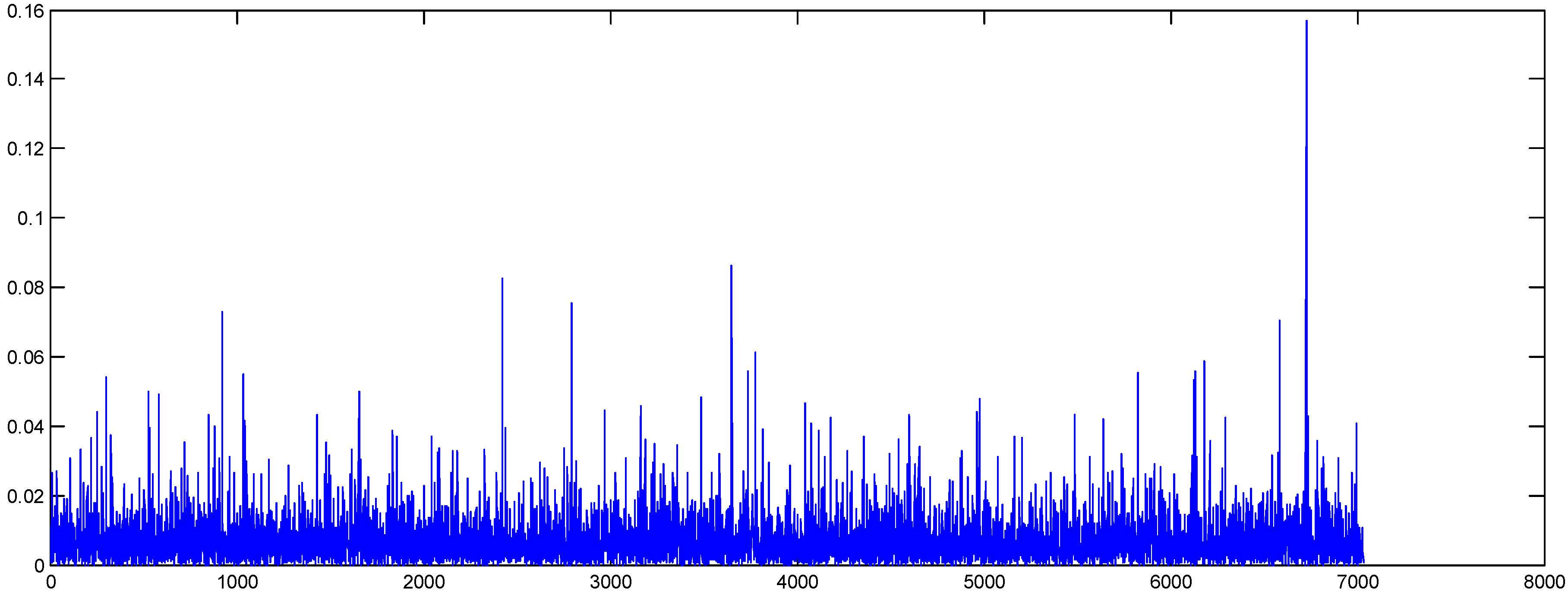
In order to determine the credibility of the different methods, we have used the shuffled version of the gold absolute return series. The original and shuffled absolute return series are presented in Figure 6 and Figure 7. As is seen from the graphs, volatility clusterings have been removed by the shuffling procedure. Our expectation is to destroy the correlations in the original series and, therefore, obtain scaling exponent H values that are close to 0.5 in the shuffled series.

Figure 6. Gold absolute returns (original data).

Figure 6. Gold absolute returns (original data).

Figure 7. Gold absolute returns (shuffled data).

Figure 7. Gold absolute returns (shuffled data).

The findings in Table 7 are obtained using the shuffled version of the gold absolute return series. Results show that, except for Higuchi’s statistic, all of the scaling exponent H values decreased to about 0.5. This situation is consistent with our theoretical expectations. In the analysis of the bull and bear periods of gold return volatilities, we use the methods that provide the closest scaling exponent H values to 0.5 in the shuffled data. These methods are the aggregated variance, Peng’s statistic and wavelet fit. However, the boxed periodogram results are surprisingly remarkable, because the scaling exponent H value is well below our theoretical expectation; it is 0.3778 for the shuffled data, whereas it is 0.6784 for the original data. In fact, these results correspond with the findings of Rea et al. [38], which state that the boxed periodogram method underestimates the scaling exponent H value.

Table 7. Robustness analysis of the scaling exponent H mols.

	Aggregated Variance	Higuchi’s Statistic	Peng’s Statistic	R/S Statistic	Boxed Periodogram	Wavelet Fit
Shuffled Gold_abs Series	0.5240 ** (0.0226) 0.0000	0.9643 ** (0.0285) 0.0000	0.4604 ** (0.0211) 0.0000	0.5380 ** (0.0333) 0.0000	0.3778 ** (0.0301) 0.0000	0.4589 ** (0.0293) 0.0000

** indicates the 95% and 99% confidence level.

Table 7. Robustness analysis of the scaling exponent H mols.

	Aggregated Variance	Higuchi’s Statistic	Peng’s Statistic	R/S Statistic	Boxed Periodogram	Wavelet Fit
Shuffled Gold_abs Series	0.5240 ** (0.0226) 0.0000	0.9643 ** (0.0285) 0.0000	0.4604 ** (0.0211) 0.0000	0.5380 ** (0.0333) 0.0000	0.3778 ** (0.0301) 0.0000	0.4589 ** (0.0293) 0.0000

** indicates the 95% and 99% confidence level.

The plot form of the results of Table 6 and Table 7 can be seen in Figure 8 below. Figure 8 presents the scaling exponent results of the original and shuffled data together. It is clear that Higuchi’s statistic value is almost the same for both data. On the other hand, as the R/S value of the original data is quite small after the shuffling procedure, there is a little change in its value. Similarly, we remember that the R/S results of the oil data are not credible. Therefore, we leave both Higuchi’s stattic and the R/S method out of the assessment in the bull and bear period analysis.

Figure 8. Original and shuffled series’ scaling exponent test results.3

Figure 8. Original and shuffled series’ scaling exponent test results.3

After determining the credible methods that will be used in the analysis of the bull and bear periods, we present the scaling exponent results for both of the business cycle phases. According to the findings in Table 8, the scaling exponents H. of the second, third and fourth bear periods are substantially higher than the bull periods. This situation demonstrates that persistency in the gold return volatility for this period is stronger than the bull periods. However, the first and the fifth periods have a different behavior; the bull periods in these business cycles have higher scaling exponent values.

The first period corresponds to the second half of 1990, whereas the fifth period coincides with the years 2008–2011. Although the aforementioned period is bull, if this period is considered in the mortgage crises duration, it is striking that there is high persistent volatility in the recovering market.

Table 8. Scaling exponent H results of the bull and bear periods of the gold data.

PANEL A	BEARS 1	BEARS 2	BEARS 3	BEARS 4	BEARS 5		BEARS 6
Aggregated Variance	0.6187 ** (0.0149) 0.0000	0.6345 ** (0.0321) 0.0000	0.8841 ** (0.0347) 0.0000	0.8632 ** (0.0422) 0.0000	0.7774 ** (0.0451) 0.0000		0.7998 ** (0.0271) 0.0000
Peng’s Statistic	0.5797 ** (0.0088) 0.0000	0.5602 ** (0.0193) 0.0000	0.6412 ** (0.0184) 0.0000	0.6541 ** (0.0244) 0.0000	0.5875 ** (0.0340) 0.0000		0.6566 ** (0.0216) 0.0000
Wavelet Fit	0.4605 (0.1630) 0.0665	0.4029 * (0.0841) 0.0409	0.4509 (0.1476) 0.0925	0.7391 ** (0.1223) 0.0090	−0.0304 (0.1712) 0.8879		0.4693 * (0.1529) 0.0490
PANEL B	BULLS 1	BULLS 2	BULLS 3	BULLS 4	BULLS 5		-
Aggregated Variance	0.9157 ** (0.0632) 0.0000	0.5053 ** (0.0789) 0.0000	0.8724 ** (0.0679) 0.0000	0.7955 ** (0.0420) 0.0000	0.8273 ** (0.0285) 0.0000		-
Peng’s Statistic	0.4384 ** (0.0243) 0.0000	0.5538 ** (0.0353) 0.0000	0.4803 ** (0.0224) 0.0000	0.6756 ** (0.0338) 0.0000	0.6949 ** (0.0366) 0.0000		-
Wavelet Fit	0.3378 * (0.0932) 0.0362	0.0414 (0.4184) 0.9370	0.2481 (0.0879) 0.2169	0.6269* (0.0487) 0.0000	0.2480 * (0.0586) 0.0241		-

* and ** indicate the 95% and 99% confidence level.

Table 8. Scaling exponent H results of the bull and bear periods of the gold data.

PANEL A	BEARS 1	BEARS 2	BEARS 3	BEARS 4	BEARS 5		BEARS 6
Aggregated Variance	0.6187 ** (0.0149) 0.0000	0.6345 ** (0.0321) 0.0000	0.8841 ** (0.0347) 0.0000	0.8632 ** (0.0422) 0.0000	0.7774 ** (0.0451) 0.0000		0.7998 ** (0.0271) 0.0000
Peng’s Statistic	0.5797 ** (0.0088) 0.0000	0.5602 ** (0.0193) 0.0000	0.6412 ** (0.0184) 0.0000	0.6541 ** (0.0244) 0.0000	0.5875 ** (0.0340) 0.0000		0.6566 ** (0.0216) 0.0000
Wavelet Fit	0.4605 (0.1630) 0.0665	0.4029 * (0.0841) 0.0409	0.4509 (0.1476) 0.0925	0.7391 ** (0.1223) 0.0090	−0.0304 (0.1712) 0.8879		0.4693 * (0.1529) 0.0490
PANEL B	BULLS 1	BULLS 2	BULLS 3	BULLS 4	BULLS 5		-
Aggregated Variance	0.9157 ** (0.0632) 0.0000	0.5053 ** (0.0789) 0.0000	0.8724 ** (0.0679) 0.0000	0.7955 ** (0.0420) 0.0000	0.8273 ** (0.0285) 0.0000		-
Peng’s Statistic	0.4384 ** (0.0243) 0.0000	0.5538 ** (0.0353) 0.0000	0.4803 ** (0.0224) 0.0000	0.6756 ** (0.0338) 0.0000	0.6949 ** (0.0366) 0.0000		-
Wavelet Fit	0.3378 * (0.0932) 0.0362	0.0414 (0.4184) 0.9370	0.2481 (0.0879) 0.2169	0.6269* (0.0487) 0.0000	0.2480 * (0.0586) 0.0241		-

* and ** indicate the 95% and 99% confidence level.

5. Conclusions

Although there is a great deal of interest in the scaling properties of the financial markets, the share of these studies in commodity markets is quite restricted. Additionally, there is no information about the scaling properties of the subperiods of the examined time series in the existing studies. As stated by Marcucci [10], financial asset returns can exhibit sudden jumps, but these jumps do not only arise from the structural breaks, but also can originate from future expectations regarding the current information level. On the other hand, in the periods of character change, even if they arise from the structural breaks or expectations, we can see different patterns in the behavior of asset returns. Therefore, rather than the whole period, modeling of the subperiods can be more beneficial in capturing the properties that can be missed when we focus on the whole series. Hence, in this study, we examined the subperiod in the analysis of scaling properties of two important commodities: gold and oil. In order to obtain the bull and bear turning points, we used the MBBQ algorithm for the period of May, 1987–March, 2014, and we determined eight bull and eight bear and five bull and six bear periods for the oil and gold markets, respectively. Using the duration, amplitude and excess measures suggested by Harding and Pagan [29] we characterized the shape and other properties of the business cycle phases. According to the results, the excess statistics of the bull and bear periods of the gold market exhibit that both of the periods have convex shapes. However, we have seen that the bear periods of the oil market are approximately linear and slightly concave, meaning that there are hard drops in the oil market, whereas the bear periods of the gold markets are more smooth and stable.

After the determination of the bull and bear markets, we performed scaling exponent H methods, which are the aggregated variance, Higuichi’s statistic, Peng’s statistic, rescaled range (R/S), boxed periodogram and wavelet fit, based on the time, frequency and wavelet domains. First, in order to determine the robustness of all of these models, we used the shuffled data and compared the results with the original data. Results showed that for both the oil and gold returns, Higuichi’ statistic, the rescaled range and the boxed periodogram models have a strong bias, whereas the aggregated variance, Peng’s statistic and wavelet fit methods are quite robust. Hence, in the closing parts of the study, we used only these three methods: the aggregated variance, Peng’s statistic and wavelet fit. The obtained scaling exponent values for the bull and bear periods demonstrated that both the oil and gold markets’ bear periods have substantially higher scaling exponent H values than the bull periods. This situation exhibits the higher volatility persistency of the bear periods. Another important finding is that both oil and gold market return volatility persistency begins to increase following the period of the mortgage crisis.