Numerical Simulations of Combustion Instabilities in a Combustor with an Augmentor-Like Geometry

Abstract

With the goal of assessing the capability of Computational Fluid Dynamics (CFD) to simulate combustion instabilities, the present work considers a premixed, bluff-body-stabilized combustor with well-defined inlet and outlet boundary conditions. The present simulations produce flow behaviors in good qualitative agreement with experimental observations. Notably, the flame flapping and standing acoustic waves seen in the experiments are reproduced by the simulations. Moreover, present predictions for the dominant instability frequency have an error of 7% and those of the rmspressure fluctuations show an error of 16%. In addition, an analysis of simulation results for the limit cycle complements previous experimental analyses by supporting the presence of an active frequency-locking mechanism.

1. Introduction

In aero gas turbine engines, the main combustor and augmentor are prone to combustion instabilities. These are resonant phenomena whose damaging effect on combustion systems is well documented [1,2]. Despite this hazard, estimating the occurrence of these phenomena is still very difficult [3,4]. Attempts to do this have led to a plethora of analytical and numerical techniques. The present interest is on one of these techniques: Computational Fluid Dynamics (CFD).

CFD has provided significant insight into the physics of combustion instabilities [5,6,7,8,9,10,11,12,13,14,15,16,17,18], which could aid in estimating them. For instance, one CFD study shows that for certain geometrical constraints simple network models are sufficient to model combustion instabilities in annular combustors [10]. Another study shows that the classic decomposition of acoustically-induced flow motions into modes may not be useful in a particular ramjet configuration [11]. In addition, another study takes advantage of the ease of specifying accurate boundary conditions in CFD (in contrast with experiments) in order to study the transition from stable to unstable combustion [8]. Similarly, yet another study identifies two potential physical mechanisms for this transition in bluff-body-stabilized-flame combustors [19].

The assessment and enhancement of this capability of CFD rest on at least two tasks. One is the continual testing of this capability using data from simple but practically-relevant combustors. The other one is the acquisition of data from combustors whose designs attempt to continually reduce the uncertainty in boundary conditions and to better approximate actual systems. With this approach in mind, and noting that the present interest is on gas-turbine augmentors, this paper considers bluff-body-stabilized-flame combustors.

Numerous experimental datasets from bluff-body-stabilized-flame combustors providing combustion-instability data are available [13,20,21,22,23,24,25,26,27,28,29,30] (see also the review by O’Connor et al. [31]). Among these datasets, those from the Limousine combustor [13,30] and the U-Melbourne combustor [26,27,28] stand out because they have several features that make them well suited to test CFD models. First, they have well-defined inlet and outlet boundary conditions, and do not use honeycomb flow-straighteners upstream of the flameholder. By well-defined it is meant here that enough information is provided to reproduce the boundary condition in a CFD simulation. In addition, they give some information about the flame together with that of the acoustics, and do so for various operating conditions. Moreover, the U-Melbourne combustor dataset is accompanied by a thorough analysis that includes the use of simple models to explain experimental trends [28,32].

Several simulation studies of the Limousine combustor have been conducted. One study identifies at a particular operating condition an interesting transition from stable to unstable combustion induced by flame flashback [13]. This mechanism has been observed in another bluff-body-stabilized-flame combustor [19] and in a swirl-stabilized-flame combustor [7]. Another study of the Limousine combustor focuses on the sensitivity of the predictions to the turbulent-combustion modeling [33]. It finds that, of the four models tested, only one reproduces experimental observations within an acceptable error. In contrast to the Limousine combustor, and to the author’s knowledge, there seems to be no CFD studies of the U-Melbourne combustor. Therefore, the present work considers this combustor.

The U-Melbourne combustor consists of a pipe with a bullet-shaped flame holder sitting inside of it. It uses a fully premixed mixture of propane and air. The inlet is choked and the outlet nozzle can have different area-ratios, $AR$. During the limit cycle, when $AR$ = 0.2–1 standing acoustic waves with a dominant frequency of 300–400 Hz are observed, and when $AR=0.1$ a bulk mode at about 85 Hz is seen. In this way, the U-Melbourne combustor offers two different types of instabilities to test CFD models. The present work focuses on the former case by using $AR=1$, leaving the study of the $AR=0.1$ case for future work.

An analysis of the experimental data using a simplified model confirms the establishment of standing acoustic waves with large values of $AR$, and explains that the production of sound when $AR=0.1$ occurs because of the impingement of entropy fluctuations (“hot spots”) on the exit nozzle [28]. However, since this model uses an empirical input for the heat-release fluctuations, it cannot be used to address which mechanisms are producing the heat-release fluctuations or why the acoustics resonate with the flow motions. The present CFD simulations are used to address these concerns and, thus, complement previous analyses from the experimentalists.

2. Approach

2.1. Governing Equations

The present work considers the following time- and spatially-averaged conservation equations for mass, momentum, total sensible enthalpy, and species for gases that are compressible, viscous, heat-conducting, multiple-component and react in a way that the heat-release-rate due to reaction is much larger than that due to viscous dissipation:

$$\frac{\partial \overline{\rho }}{\partial t}+\frac{\partial \left(\overline{\rho }{\tilde{u}}_i\right)}{\partial x_i}={\mathcal{S}}_{\rho },$$

(1)

$$\frac{\partial \overline{\rho }{\tilde{u}}_i}{\partial t}+\frac{\partial \left(\overline{\rho }{\tilde{u}}_j{\tilde{u}}_i\right)}{\partial x_j}=-\frac{\partial \overline{p}}{\partial x_i}+\frac{\partial }{\partial x_j}\left({\overline{\tau }}_{ji}+{\tau }_{ji}^{sgs}\right)+{\mathcal{S}}_{U,i},$$

(2)

$$\frac{\partial \overline{\rho }\tilde{H}}{\partial t}+\frac{\partial (\overline{\rho }{\tilde{u}}_j\tilde{H})}{\partial x_j}=-\frac{\partial }{\partial x_j}\left({\overline{q}}_j+q_j^{sgs}\right)+\frac{\partial \overline{p}}{\partial t}+{\overline{S}}_H+{\mathcal{S}}_H,$$

(3)

$$\frac{\partial \overline{\rho }{\tilde{Y}}_{\alpha }}{\partial t}+\frac{\partial (\overline{\rho }{\tilde{u}}_j{\tilde{Y}}_{\alpha })}{\partial x_j}=-\frac{\partial }{\partial x_j}\left({\overline{j}}_{\alpha ,j}+j_{\alpha ,j}^{sgs}\right)+{\overline{S}}_{\alpha }+{\mathcal{S}}_{Y_{\alpha }}.$$

(4)

Here, $\rho$ is the density, p is the pressure, $u_i$ is the velocity vector, H is the total enthalpy defined as $H=h_s+0.5u_i{u}_i$ with $h_s$ the sensible enthalpy, and $Y_{\alpha }$ is the mass fraction of the species $\alpha$. The bar denotes an average and the tilde a Favre average. ${\overline{\tau }}_{ji}$, ${\overline{q}}_j$, and ${\overline{j}}_{\alpha ,j}$ are, respectively, the averaged viscous stress tensor, heat flux, and Fickian molecular flux of species $\alpha$. Similarly, ${\tau }_{ji}^{sgs}$, $q_j^{sgs}$, and $j_{\alpha ,j}^{sgs}$ are the subgrid viscous stress tensor, heat flux, and molecular flux of species $\alpha$, all of which need closure. The rightmost terms on the right-hand side of Equations (1)–(4) are zero everywhere except in a sponge zone, as discussed below. These conservation equations are complemented with the averaged equation of state for ideal gases,

$$\overline{p}=\overline{\rho }{R}_u\sum _{\alpha =1}^N\frac{{\tilde{Y}}_{\alpha }\tilde{T}}{M{W}_{\alpha }},$$

(5)

and the averaged caloric equation of state given by NASA polynomials, ${\tilde{h}}_s={\tilde{h}}_s(\tilde{T})$. $R_u$ is the universal gas constant, $M{W}_{\alpha }$ is the molecular weight of the species $\alpha$, and T is the temperature.

Kinematic viscosity and thermal and mass diffusivities are taken to be all equal and given by Sutherland’s formula. The subgrid terms ${\tau }_{ji}^{sgs}$, $q_j^{sgs}$, and $j_{\alpha ,j}^{sgs}$ are closed with the one-equation-eddy model [34] (implementation details are given elsewhere [35]), and with the use of turbulent Prandtl and Schmidt numbers equal to one. The averaged chemical source terms ${\overline{S}}_H$ and ${\overline{S}}_{\alpha }$ are closed with the partially-stirred-reactor (PaSR) model.

With the PaSR model, the averaged chemical source term, ${\overline{S}}_{\alpha }$, is computed with [36]

$${\overline{S}}_{\alpha }=\left(\frac{{\tau }_c}{{\tau }_c+{\tau }_m}\right)\left(\frac{C_{\alpha }^{*}-{\overline{C}}_{\alpha }}{\Delta t}\right)M{W}_{\alpha },$$

(6)

where ${\overline{C}}_{\alpha }=\overline{\rho }{\tilde{Y}}_{\alpha }/M{W}_{\alpha }$, ${\tau }_c$ is a chemical characteristic time defined to be proportional to an average of the forward reaction rate of all reactions and all species. ${\tau }_m$ is the mixing characteristic time given by:

$${\tau }_m=c_{mix}\sqrt{\frac{\overline{\mu }+{\mu }^{sgs}}{\overline{\rho }{ϵ}^{sgs}}},$$

(7)

with $c_{mix}$ being a model constant equal to one here, ${\mu }^{sgs}$ a subgrid-scale eddy viscosity, and ${ϵ}^{sgs}$ a subgrid-scale dissipation. An important feature of the PaSR model is the computation of $C_{\alpha }^{*}$, which represents the concentration of the species $\alpha$ at the subgrid level. $C_{\alpha }^{*}$ is computed from the solution of the governing equations of a constant-pressure reactor [37]. For this solution, ${\overline{C}}_{\alpha }$ and $\tilde{T}$ are used as initial conditions, and the simulation is time-advanced from t to $t+\Delta t$ at time intervals of the order of ${\tau }_c$. More details about the PaSR model are given elsewhere [36].

The modeling approach explained above is fully compressible. However, two incompressible simulations are used to interpret the CFD instability results. With this incompressible or low-Mach-number formulation, the governing equations are Equations (1)–(7), but with $\overline{p}=p_0$ in Equation (5) and $p_0$ being a reference pressure, equal to one atmosphere in the present work, and Equation (3) replaced by:

$$\frac{\partial \overline{\rho }{\tilde{h}}_s}{\partial t}+\frac{\partial (\overline{\rho }{\tilde{u}}_j{\tilde{h}}_s)}{\partial x_j}=-\frac{\partial }{\partial x_j}\left({\overline{q}}_j+q_j^{sgs}\right)+{\overline{S}}_H.$$

(8)

In the incompressible simulations, the rightmost terms on the right-hand side of Equations (1)–(4) are always zero.

2.2. Numerical Method

The governing equations are solved with reactingFoam^® (v. 2.3.1), the reacting solver of the OpenFOAM^® library [38,39]. This solver is transient, compressible, and pressure-based. It uses an inner iterative loop to correct the velocity field using the output of a pressure equation, as in the well-known PISO algorithm [40], and also uses an outer iteration loop for additional corrections. Various temporal and spatial discretization options are available for reactingFoam. In the present work, time is discretized with a second-order backward-differencing scheme that uses the current and previous two time-step values. A time-step of 4E-8 is used. Inviscid fluxes are computed using a blended central/upwind scheme called limited-linear. Verification of these numerics is provided elsewhere [41,42,43,44]. Finally, note that OpenFOAM solvers or earlier versions have been observed to reproduce satisfactory results in a large variety of combustion problems [19,39,45,46,47,48,49,50,51].

2.3. Configuration

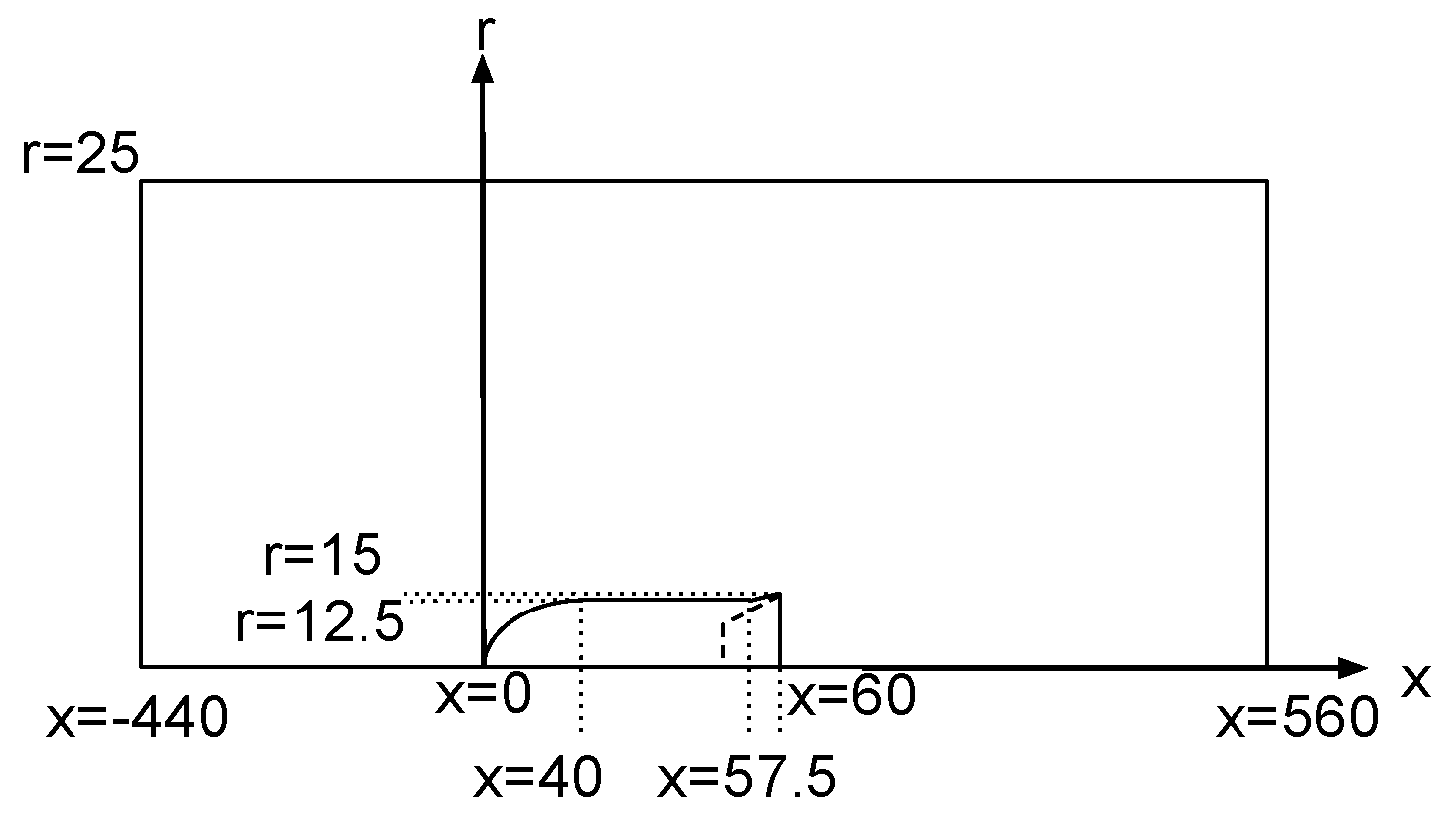
The U-Melbourne combustor consists of a pipe that is 1000 mm long and has a diameter of 50 mm. A bullet-shaped flame holder sits inside the pipe, as indicated in Figure 1. Geometric details of this flame holder are given elsewhere [32] and in the Supplementary Materials. The outlet nozzle can have different area-ratios. The present work considers the designs with an area-ratio ($AR$) of one. The computational domain includes the geometry in Figure 1 and a portion of the ambient gas, as discussed shortly. Unless said otherwise, the discussion focuses on simulations using a baseline mesh with 530,000 tetrahedral cells that is refined near the wake of the flame-holder to about 2 mm and near the walls. Simulations using a coarser mesh of 218,000 cells are also discussed.

The inlet plane, $x=-$440 mm, is choked. Through it flows a premixed mixture of propane and air. Various inlet conditions are available. The ones used here for $AR=1$ are 14.87 m/s, 344 K, and an equivalence ratio of 0.9. Inside the combustor, the pressure is atmospheric. A one-step chemical mechanism is used [52]. Walls are no-slip and isothermal at 700 K.

The outlet is open to the atmosphere and it is modeled using a sponge method [53]. With this method, the computational domain includes the geometry shown in Figure 1 and a so-called sponge zone downstream. This sponge zone is a hemisphere with a radius of $R_{max}=0.4$ m, and it is centered at the intersection of the combustor axis and the outlet plane $x_0=0.56$ m. The flat boundary of this hemisphere is considered a wall, and the rest of its boundary is modeled with OpenFOAM’s wave-transmissive boundary condition. Such a hemisphere is intended to mimic the effect of an unbounded domain. This is done by using the following source terms on the right-hand sides of Equations (1)–(4), respectively: ${\mathcal{S}}_{\rho }=\sigma ({\rho }_0-\rho )$; ${\mathcal{S}}_{U,i}=\sigma ({\rho }_0{u}_{i,0}-\rho u_i)$; ${\mathcal{S}}_H=\sigma ({\rho }_0{H}_0-\rho H)$; and ${\mathcal{S}}_{Y_{\alpha }}=\sigma ({\rho }_0{Y}_{\alpha ,0}-\rho Y_{\alpha })$. Here, $\sigma =A_s{R}^2/R_{max}^2$ with $A_s=$1000 and $R^2=({(x-x_0)}^2+r^2$). Quantities with a subindex 0 denote (constant) reference values corresponding to ambient air with a very small horizontal velocity (0.027 m/s).

To complete the specification of the outlet boundary condition, OpenFOAM’s wave-transmissive boundary condition is briefly explained. This boundary condition solves the following equation for pressure at some specified surface, here the outlet surface of the hemisphere:

$$\frac{\partial \overline{p}}{\partial t}+U\frac{\partial \overline{p}}{\partial x_n}=K(p_{\infty }-\overline{p}),$$

(9)

where $U=u_c+c_0$, $u_c$ is a characteristic convective speed, $c_0$ is a reference speed of sound, $x_n$ is normal to the boundary, $K=U/l_{\infty }$, and $p_{\infty }$ is the pressure outside the boundary, evaluated at a distance $l_{\infty }$. At values of $l_{\infty }$ that are small enough, this boundary condition acts as a reflective boundary condition, whereas, for large enough values, it is approximately nonreflecting. More precisely, this boundary condition acts as a low-pass filter with cutoff frequency of $\beta K$ [54], with $\beta$ being a constant of order 1. Here, $l_{\infty }$ = 0.1 m.

With the incompressible or low-Mach-number simulations, there is no need for the sponge zone. At the outlet of these simulations, velocity, temperature and species are set to a zero-normal-gradient condition or a fixed value, depending on the direction of the flow. Pressure is dealt with in a similar way.

3. Results

Before discussing results for the main simulation, some commentary about the selection of the above CFD-model parameters is necessary. Only a brief discussion is provided since a full one could be a paper on its own. Turbulence-transport models, such as the one-equation-eddy model, were found to be necessary because not using them produced flame stabilization upstream of the flame-holder, unlike what is seen in the experiments. Preference was given to the one-equation-eddy model over the widely-used Smagorinsky model because, in previous simulations of a similar bluff-body-stabilized flame, the former gave a flame shape in better agreement with experiments [51]. The mesh spacings in these past simulations are within those used here. Regarding the present meshes, their type and spacings were selected in a way to mimic meshes that could potentially be used in a more realistic combustor. The sponge method was used because it allowed predictions of the rms pressure fluctuations in better agreement with the experiments in comparison with ending the domain at the $x=560$ mm plane (see Figure 1) and using the wave-transmissive boundary condition at this plane. This is not surprising since the sponge method better mimics the open-to-ambient boundary condition. Note that more advance treatments of the outlet are available [55,56]. However, as shown below, the sponge method was found to be sufficient for the present purposes. No tuning of the sponge-method parameters was attempted. In contrast, some tuning of the wall temperature was necessary because this boundary condition is unknown from the experiments. This is unavoidable. In fact, this boundary condition is unknown in all the experimental datasets considered for the present work (see Section 1). When considering wall temperatures between the inlet temperature and the flame temperature, it was found that those near the former produced dominant frequencies of the instability that were too low, while those near the latter produced flame flashback along the combustor walls, something not seen in the experiments. The in-between value of 700 K was found to be adequate and used in the baseline simulation of this paper.

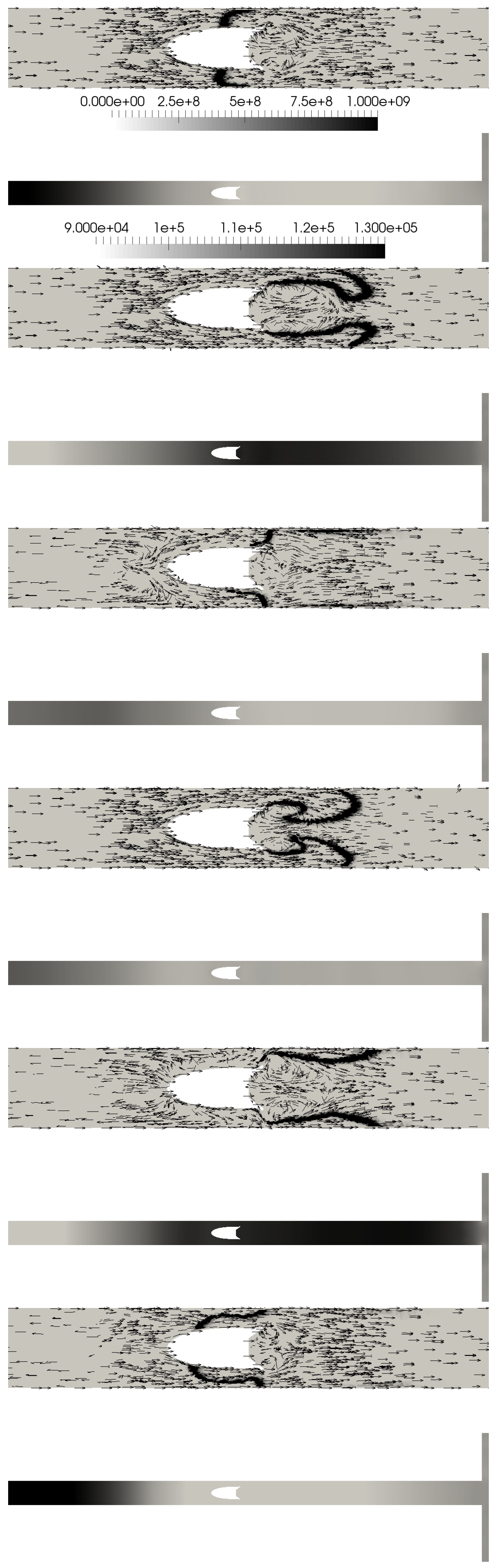
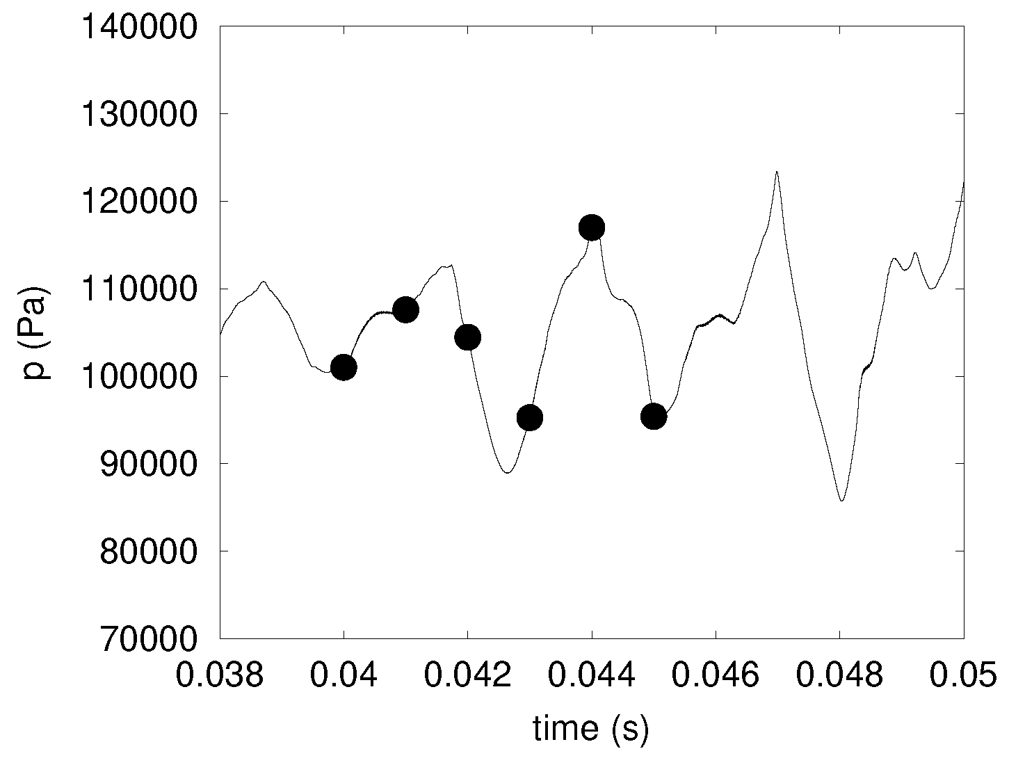
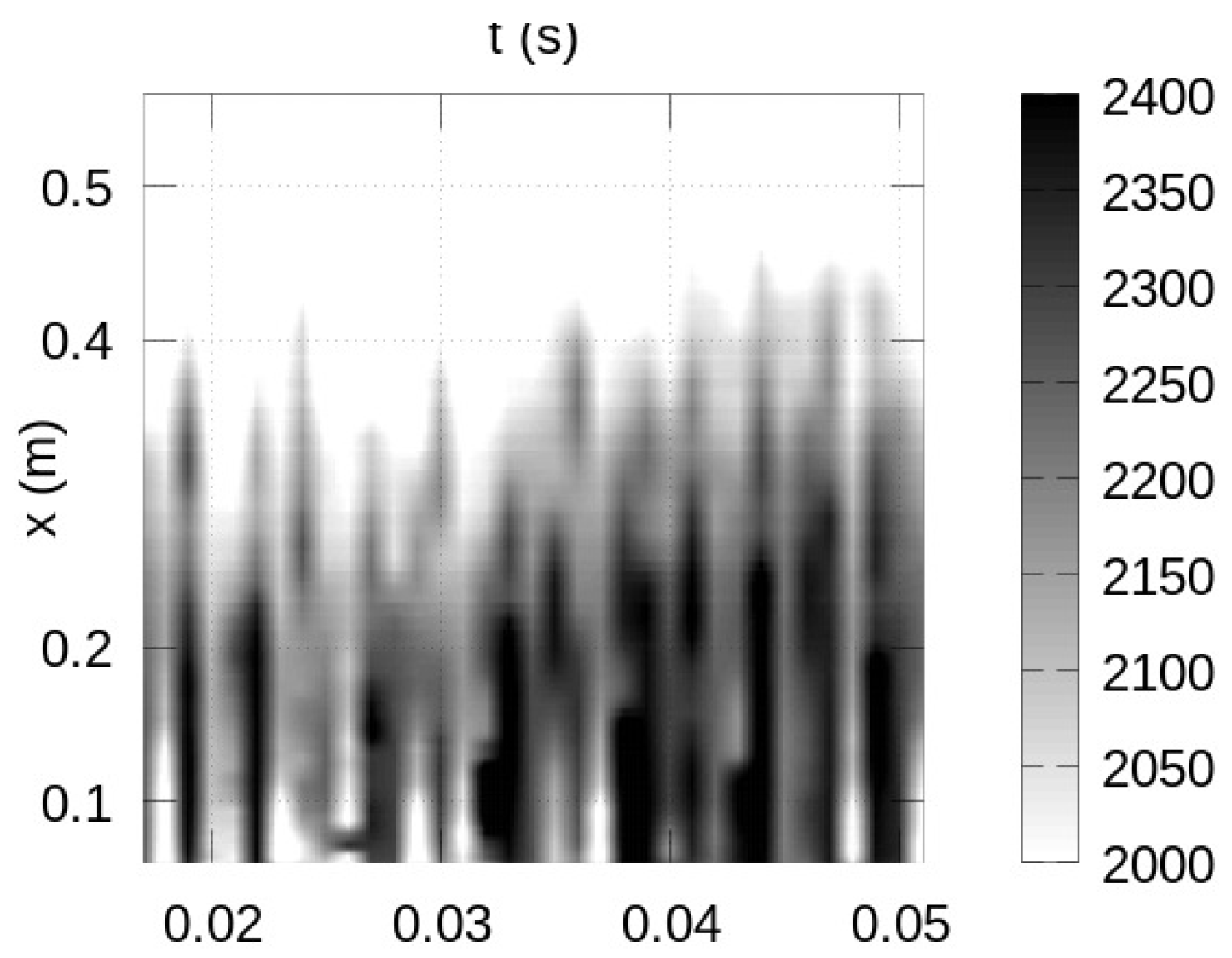
Moving on to the limit-cycle results for the main simulation of the present work, Figure 2 presents instantaneous maps of heat release rate and pressure at a plane dividing the tube in two equal sections. Superimposed velocity vectors are also shown. The corresponding times are indicated with symbols in the time trace of pressure in Figure 3. The heat-release-rate maps in Figure 2 show that the flame flaps in the streamwise direction. This flapping can be better seen in Figure 4, which shows the centerline temperature in space-time: Notice the variation of temperature along the time coordinate downstream of the flameholder. (The downstream face of the flameholder is at $x=0.06$ m.) For another look at this flapping, a movie is available in the Supplementary Materials. Such a flapping movement of the flame is consistent with experimental observations [28,32].

Figure 2 also shows some flashback of the flame around the flameholder, at the first and sixth frames from top to bottom, when a minimum pressure occurs (see Figure 3). In fact, the velocity vectors in Figure 2 show reverse flow near the flameholder, which is more clearly seen in the fifth frame from top to bottom, as well as further upstream. This observation is consistent with the “significant reversed flow during some parts of the cycle” [28] seen in the experiments, as well as in a previous similar experiment [57].

Further insight into the instability can be obtained by looking at the terms of Rayleigh’s inequality [58,59]:

$$\frac{1}{\tau }{\int }_{\tau }{\int }_V\left(\frac{\gamma -1}{\gamma p_0}{p}^{\prime }{q}^{\prime }\right)dVdt>\frac{1}{\tau }{\int }_{\tau }{\int }_A\left(p^{\prime }{u}^{\prime }\right)dAdt.$$

(10)

Here, $\tau$ is a time interval that includes several instability cycles; V is the volume of the combustor; $\gamma$ is the ratio of specific heats, which is taken as constant and equal to 1.35; $p_0$ is a reference pressure, which is taken as atmospheric; $p^{\prime }$ denotes pressure fluctuations; $q^{\prime }$ denotes heat release fluctuations; $u^{\prime }$ denotes velocity fluctuations normal to the combustor outlet(s); and A is the area of the combustor outlet(s). The term between parenthesis on the left-hand side of Equation (10) is termed the Rayleigh index.

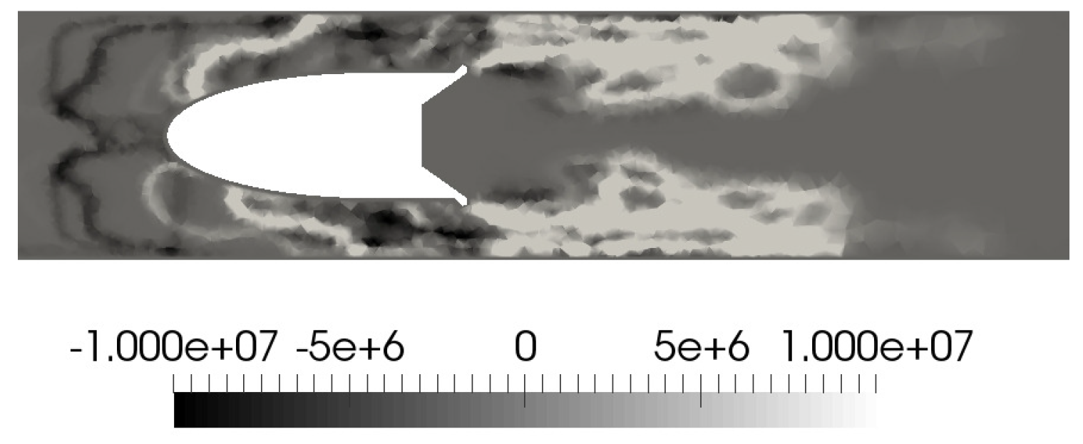
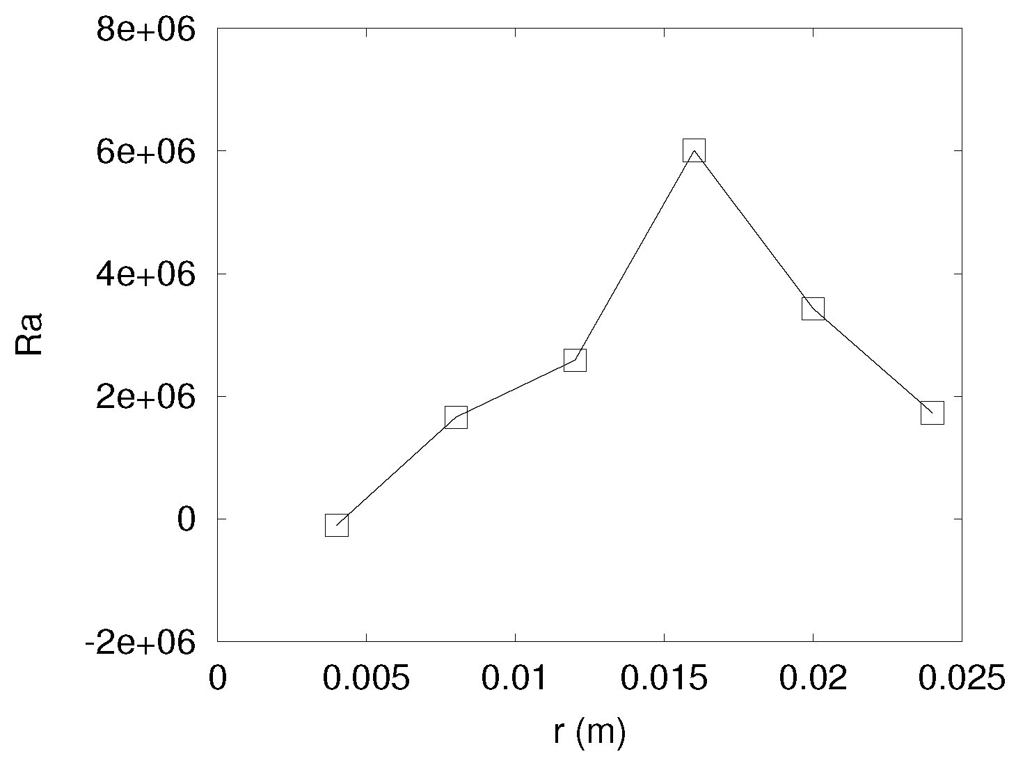
Figure 5 shows a map of the Rayleigh index at a plane dividing the tube in two equal sections. Positive (negative) values of the Rayleigh index indicate a region where the combustion instability is being driven (damped). Figure 5 shows a strong driving of the instability (light regions) right downstream of the flameholder where the flame flaps, as well as some damping (dark regions) where the flame undergoes flashback. A closer inspection shows that there is a particularly strong driving at the edges of the wake. This can be better seen in Figure 6, which shows the radial variation of the spatially-averaged Rayleigh index. This average is done over the circumferential direction and in the region $-0.05<x<0.15$ m. Note that the radius of the bluff body is 0.015 m.

In terms of the budget associated with Equation (10), the simulations show that the left-hand side is about 1000 W while the right-hand side is about 100 W. Therefore, since there are no strong damping process associated with viscous phenomena, such as the production of vorticity in perforated plates [60,61], this difference suggests the presence of a combustion instability in the present problem.

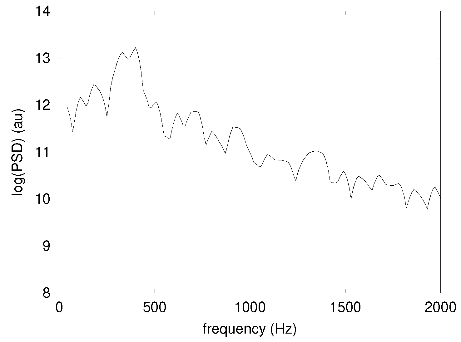
The power spectral density (PSD) obtained by averaging at different locations along the centerline is shown in Figure 7. Notice a dominant frequency, i.e., that associated with the largest peak in PSD, of 390 Hz, and other harmonics at approximately 187, 513, and 712 Hz. In comparison, the experimental work reports a dominant frequency of 364 Hz (Figure 5.4b in Hield [32]), and other modes at 197, 560, and 729 Hz. The error in the prediction of the dominant frequency is 7 %.

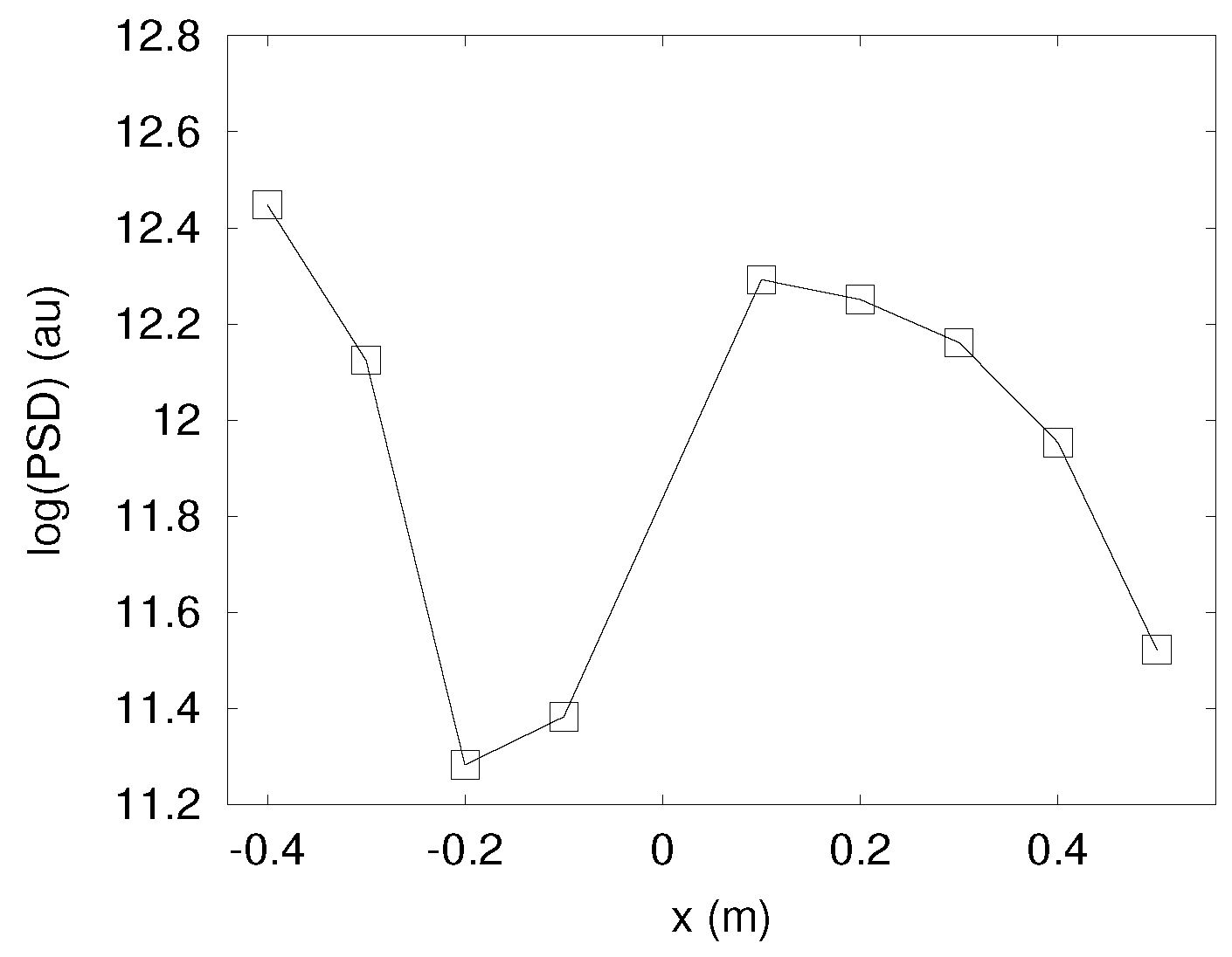
The spatial variation of pressure is observed to occur mainly along the streamwise direction, as can be seen in Figure 2. This variation is shown in Figure 8 by plotting the value of the PSD at the dominant frequency at different axial locations and at the centerline. Notice there is a pressure antinode at the inlet and another one near the flameholder, and a pressure node at the outlet. Such a variation is consistent with that seen in the experiments (Figure 5.3 Hield [32]).

Regarding the magnitude of the pressure-fluctuations amplitude, the experimentalists report a rms value of about 14,000 near the flameholder (estimated from Table 5.1 and Figure 6.7 in Hield [32] for $\varphi =0.9$), at $x=28$ mm and at the wall. At this location, the simulations show a rms value of around 16,300 Pa. The error in the prediction of rms pressure fluctuations is 16%.

With the coarse mesh, the above flow motions are also reproduced, the observed dominant frequency is 398 Hz, and rms pressure fluctuations are 19,000 Pa. Thus, in comparison with the experiments, the dominant frequency prediction is 9% larger, and the rms pressure fluctuations are 36% larger.

To report the computational cost, consider as a metric the cpu-hours of computing time per second of simulation time and per number of cells, $cpu-h/(s-cells)$. The present simulation costs 0.3 $cpu-h/(s-cells)$. When using as a metric cpu-hours per 1000 cycles of the instability based on the dominant frequency and per number of cells, $cpu-h/(1000cycle-cells)$, the cost of present simulations is 0.8. In comparison, in other studies the value of $cpu-h/(s-cells)$ is as follows: 3 in Harvazinski et al. [62], 0.17 in Hernandez [63], and 0.1 in Wolf et al. [9]. As in the present simulations, Hernandez [63] and Wolf et al. [9] used a turbulent-combustion model, a global mechanism, a time step of O(1E-8) s, and a (predominantly) tetrahedral mesh. Harvazinski et al. [62] also used a global mechanism (their results for a detailed mechanism are not considered here), but used no turbulent-combustion model, and a time step of O(1E-7) s. Therefore, the cost of present simulations in $cpu-h/(s-cells)$ is within that of previous studies.

4. Analysis

The present analysis focuses on the limit cycle. In this case, one question that arises is as follows: What is the nature of the acoustics in the chamber? This question was elegantly addressed by Hield et al. [28] using a simplified model. This model shows that when $AR=1$ the acoustics result from standing waves, while in the $AR=0.1$ case there is a bulk mode and the acoustics result from the impingement of entropy fluctuations (“hot spots”) on the exit nozzle. However, since this simplified model uses an empirical input for the heat-release fluctuations, it cannot be used to address the following questions: Which are the mechanisms producing the heat-release fluctuations? Why do the acoustics resonate with the flow motions?

In response to the first question, the experimentalists report that flame luminosity images show that, during the instability, the “flame grows from a small kernel just downstream of the flameholder” [28]. This suggests that the flame has undergone a strong extinction. Flame extinction can be seen in Figure 2 as the reduction in size and intensity of heat-release-rate contours. For example, notice in the second (from top to bottom) heat-release-rate contour in Figure 2 a large black region. This indicates a strong heat release rate. In contrast, note that the size of the black region is much smaller in the third (from top to bottom) heat-release-rate contour. The contrast between these two contours, taken at different times during the instability, indicate that the flame has undergone extinction. To take another look, consider Figure 4. Notice the time variation of the temperature along the tube centerline. Such variation is up to 400 K. Together with Figure 2, this temperature variation in Figure 4 suggests the presence of flame extinction during the instability. Furthermore, an inspection of Figure 2 shows that the flame is in contact with the wall at some instances during the instability. In particular, note the third (from top to bottom) heat-release-rate contour. Focusing on Figure 5, notice regions of strong driving and damping next to the combustor walls. This suggests that flame–wall interactions play a role in the generation of heat-release fluctuations during the limit cycle. Such a role has been observed in other combustors [19,64]. Therefore, present simulation results complement the experimental observations in identifying extinction as an important mechanism of heat-release fluctuations in the present case, and highlight the role of flame–wall interactions.

To address the second question above, additional simulations are needed. Note that what follows is an approximate analysis intended solely to provide insight. For two incompressible (or low-Mach-number-formulation) simulations, Figure 9 shows the temporal evolution of the vertical velocity near the wake (not at the centerline). Both of these simulations use the same parameters of the baseline simulation but without the sponge zone (see Section 2). One is for a non-reacting flow, and the other one is for a reacting flow. Being incompressible, no acoustic waves are produced. Thus, the time variation shown in Figure 9 is entirely hydrodynamic. Notice that, whereas the vertical velocity in Figure 9a fluctuates strongly (amplitude of the order of 1 m/s) in the non-reacting case, in Figure 9b, it fluctuates only slightly (amplitude of the order of 0.01 m/s) in the reacting case. This stabilization effect of combustion is well known [65]. In the non-reacting case, the fluctuations show dominant frequencies of about 73 Hz, and second harmonics at about 139 Hz.

The wake frequencies of the non-reacting incompressible simulation are representative of the $AR=1$ case because the same conditions are used. They are also representative of the $AR=0.1$ because the inlet velocities in the $AR=1$ (14.87 m/s) and $AR=0.1$ (13.88 m/s) cases are about the same. These wake frequencies are within the observed instability frequencies for both the $AR=1$ (see above) and $AR=0.1$ (85 Hz dominant frequency from the experiments) cases. Hence, it is likely for the so-called frequency-locking mechanism to be active.

According to this mechanism, if the forcing of a bluff-body-stabilized flame is strong enough, and its frequency is close enough to the natural wake frequency, then the resultant flow fluctuations will occur at the forcing frequency [66]. How close these frequencies should be for the locking to occur depends on the amplitude of the forcing and the density ratio of burnt and unburnt gases (cf. Figure 12 in Emerson et al. [67]). (These frequencies do not necessarily have to be the same, an issue that tends to be confused.) In addition, the amplitude of the resultant flow fluctuations is larger the closer the forcing frequency is to the wake frequency (cf. Figure 17 in Emerson et al. [67]). In the present context, this forcing is produced by the acoustics.

To provide further evidence that the frequency-locking mechanism is indeed active, a simulation similar to that of the $AR=1$ case above was run but using a shorter domain: $-0.096<x<0.204$ m (see Figure 1). An instability is seen in this case with a frequency of 500 Hz. This lower frequency is expected since the length of the combustor has been shortened. More interestingly, the rms pressure fluctuations are about seven times lower than in the baseline $AR=1$ case. Thus, a forcing frequency further away from the wake frequency leads to smaller pressure fluctuations. This result supports the presence of the frequency-locking mechanism.

5. Conclusions

The present work is a numerical study of combustion instabilities in the U-Melbourne combustor, a combustor with an augmentor-like geometry. For the purpose of testing CFD models, this combustor has the attractive features of having well-defined (as defined in Section 1) inlet and outlet boundary conditions. To the author’s knowledge, this is the first numerical study of the flow in the U-Melbourne combustor.

The present CFD simulations of the unity-nozzle-aspect-ratio case predict a flapping of the premixed flame during the limit cycle, and a standing wave mode with antinodes at the inlet and near the flameholder. Both of these observations are seen in the experiments. Moreover, the present predictions for the dominant instability frequency have an error of 7%, and those of the rms pressure fluctuations show an error of 16%. These results were obtained with a readily-available code, reactingFoam^®, and with a computational cost in $cpu-h/(s-cells)$ of 0.3, which is within that of other codes.

An analysis of the CFD data during the limit cycle shows that flame extinction plays a role in the generation of heat-release fluctuations. In addition, the CFD simulations support the hypothesis that the frequency-locking mechanism couples the combustor acoustics with the flow motions in the wake. This closes the resonant loop between acoustics and heat-release fluctuations. In this way, an analysis of CFD results complements the previous analysis of experimental data.

Finally, the present results confirm the strong sensitivity of combustion instabilities to the boundary conditions, wall temperatures in this case.

Next steps could include addressing the following questions: How well can the present performance of CFD for an academic combustor be reproduced for a combustor better resembling gas-turbine augmentors? For this purpose, how can we satisfactorily model more complex boundary conditions such as perforated plates and a turbine–stator system?

References

- Culick, F.E. Unsteady Motions in Combustion Chambers for Propulsion Systems; Research and Technology Organisation/North Atlantic Treaty Organisation: Neuilly, France, 2006. [Google Scholar]
- Lieuwen, T.C.; Yang, V.; Lu, F.K. Combustion Instabilities in Gas Turbine Engines: Operational Experience, Fundamental Mechanisms and Modeling; American Institute of Aeronautics and Astronautics: Washington, DC, USA, 2005. [Google Scholar]
- Yang, V. Liquid Rocket Engine Combustion Instability; American Institute of Aeronautics and Astronautics: Washington, DC, USA, 1995; Volume 169. [Google Scholar]
- Poinsot, T. Prediction and Control of Combustion Instabilities in Real Engines. Proc. Combust. Inst. 2017, 36, 1–28. [Google Scholar] [CrossRef]
- Menon, S. Active Control of Combustion Instability in a Ramjet Using Large Eddy Simulations; AIAA Paper 1991-0411; AIAA: Reston, VA, USA, 1991. [Google Scholar]
- Möller, S.; Lundgren, E.; Fureby, C. Large Eddy Simulation of Unsteady Combustion. Symp. (Int.) Combust. 1996, 26, 241–248. [Google Scholar] [CrossRef]
- Huang, Y.; Sung, H.; Hsieh, S.; Yang, V. Large-Eddy Simulation of Combustion Dynamics of Lean-Premixed Swirl-Stabilized Combustor. J. Propuls. Power 2003, 19, 782–794. [Google Scholar] [CrossRef] [Green Version]
- Martin, C.E.; Benoit, L.J.; Sommerer, Y.; Nicoud, F.; Poinsot, T. Large-Eddy Simulation and Acoustic Analysis of a Swirled Staged Turbulent Combustor. AIAA J. 2006, 44, 741–750. [Google Scholar] [CrossRef]
- Wolf, P.; Staffelbach, G.; Roux, A.; Gicquel, L.; Poinsot, T.; Moureau, V. Massively Parallel LES of Azimuthal Thermo-Acoustic Instabilities in Annular Gas Turbines. C. R. Mec. 2009, 337, 385–394. [Google Scholar] [CrossRef]
- Staffelbach, G.; Gicquel, L.; Boudier, G.; Poinsot, T. Large Eddy Simulation of Self Excited Azimuthal Modes in Annular Combustors. Proc. Combust. Inst. 2009, 32, 2909–2916. [Google Scholar] [CrossRef]
- Gicquel, L.Y.M.; Roux, A. LES to Ease Understanding of Complex Unsteady Combustion Features of Ramjet Burners. Flow Turbul. Combust. 2011, 87, 449–472. [Google Scholar] [CrossRef]
- Wolf, P.; Balakrishnan, R.; Staffelbach, G.; Gicquel, L.; Poinsot, T. Using LES to Study Reacting Flows and Instabilities in Annular Combustion Chambers. Flow Turbul. Combust. 2012, 88, 191–206. [Google Scholar] [CrossRef]
- Hernández, I.; Staffelbach, G.; Poinsot, T.; Román Casado, J.C.; Kok, J. LES and Acoustic Analysis of Thermo-Acoustic Instabilities in a Partially Premixed Model Combustor. C. R. Mec. 2013, 341, 121–130. [Google Scholar] [CrossRef]
- Harvazinski, M.E.; Talley, D.G.; Sankaran, V. Comparison of Laminar and Linear Eddy Model Closures for Combustion Instability Simulations; AIAA Paper 2015-3842; AIAA: Reston, VA, USA, 2015. [Google Scholar]
- Harvazinski, M.E.; Huang, C.; Sankaran, V.; Feldman, T.W.; Anderson, W.E.; Merkle, C.L.; Talley, D.G. Coupling between Hydrodynamics, Acoustics, and Heat Release in a Self-Excited Unstable Combustor. Phys. Fluids 2015, 27, 045102. [Google Scholar] [CrossRef]
- Bauerheim, M.; Staffelbach, G.; Worth, N.A.; Dawson, J.R.; Gicquel, L.Y.M.; Poinsot, T. Sensitivity of LES-based harmonic flame response model for turbulent swirled flames and impact on the stability of azimuthal modes. Proc. Combust. Inst. 2015, 35, 3355–3363. [Google Scholar] [CrossRef] [Green Version]
- Ghani, A.; Poinsot, T.; Gicquel, L.; Staffelbach, G. LES of Longitudinal and Transverse Self-excited Combustion Instabilities in a Bluff-body Stabilized Turbulent Premixed Flame. Combust. Flame 2015, 162, 4075–4083. [Google Scholar] [CrossRef]
- Ghani, A.; Miguel-Brebion, M.; Selle, L.; Duchaine, F.; Poinsot, T. Effect of Wall Heat Transfer on Screech in a Turbulent Premixed Combustor. In Proceedings of the Summer Program of the Center for Turbulence Research; Center for Turbulence Research: Stanford, CA, USA, 2016; p. 133. [Google Scholar]
- Gonzalez-Juez, E.D. Numerical Simulations of Screech; AIAA Paper 2015-3965; AIAA: Reston, VA, USA, 2015. [Google Scholar]
- Rogers, D.E.; Marble, F.E. A Mechanism for High-Frequency Oscillation in Ramjet Combustors and Afterburners. J. Jet Propuls. 1956, 26, 456–462. [Google Scholar] [CrossRef] [Green Version]
- Elias, I. Acoustical Resonances Produced by Combustion of a Fuel-Air Mixture in a Rectangular Duct. J. Acoust. Soc. Am. 1959, 31, 296–304. [Google Scholar] [CrossRef]
- Langhorne, P.J. Reheat Buzz: An Acoustically Coupled Combustion Instability. Part 1. Experiment. J. Fluid Mech. 1988, 193, 417–443. [Google Scholar] [CrossRef]
- Sjunnesson, A.; Nelson, C.; Max, E. LDA Measurements of Velocities and Turbulence in a Bluff Body Stabilized Flame. In Proceedings of the 4th International Conference on Laser Anemometry, Cleveland, OH, USA, 5–9 August 1991. [Google Scholar]
- Chakravarthy, S.R.; Sivakumar, R.; Shreenivasan, O.J. Vortex-Acoustic Lock-on in Bluff-Body and Backward-Facing Step Combustors. Sadhana 2007, 32, 145–154. [Google Scholar] [CrossRef]
- Cuppoletti, D.R.; Kastner, J.; Reed, J., Jr.; Gutmark, E.J. High Frequency Combustion Instabilities with Radial V-Gutter Flameholders; AIAA Paper 2009-1176; AIAA: Reston, VA, USA, 2009. [Google Scholar]
- Hield, P.A.; Brear, M.J. A Laboratory Combustor for Studies of Premixed Combustion Instability. In Proceedings of the 16th Australasian Fluid Mechanics Conference (AFMC), School of Engineering, The University of Queensland, Brisbane, Australia, 3–7 December 2007; pp. 99–103. [Google Scholar]
- Hield, P.A.; Brear, M.J. Comparison of Open and Choked Premixed Combustor Exits During Thermoacoustic Limit Cycle. AIAA J. 2008, 46, 517–526. [Google Scholar] [CrossRef]
- Hield, P.A.; Brear, M.J.; Jin, S. Thermoacoustic Limit Cycles in a Premixed Laboratory Combustor with Open and Choked Exits. Combust. Flame 2009, 156, 1683–1697. [Google Scholar] [CrossRef]
- Song, J.; Jung, C.; Hwang, J.; Yoon, Y. An Experimental Study on the Flame Dynamics with V-Gutter Type Flameholder in the Model Combustor; AIAA Paper 2011-6126; AIAA: Reston, VA, USA, 2011. [Google Scholar]
- Roman Casado, J.C. Nonlinear Behavior of the Thermo Acoustic Instabilities in the Limousine Combustor. Ph.D. Thesis, University of Twente, Enschede, The Netherlands, 2013. [Google Scholar]
- O’Connor, J.; Acharya, V.; Lieuwen, T. Transverse Combustion Instabilities: Acoustic, Fluid Mechanic, and Flame Processes. Prog. Energy Combust. Sci. 2015, 49, 1–39. [Google Scholar] [CrossRef]
- Hield, P.A. An Experimental and Theoretical Investigation of Thermoacoustic Instability in a Turbulent Premixed Laboratory Combustor. Ph.D. Thesis, University of Melbourne, Melbourne, Australia, 2007. [Google Scholar]
- Shahi, M.; Kok, J.; Pozarlik, A.K.; Casado, J.C.R.; Sponfeldner, T. Sensitivity of the Numerical Prediction of Turbulent Combustion Dynamics in the LIMOUSINE Combustor. J. Eng. Gas Turbines Power 2014, 136, 021504. [Google Scholar] [CrossRef]
- Yoshizawa, A.; Horiuti, K. A Statistically-Derived Subgrid-Scale Kinetic Energy Model for the Large Eddy Simulation of Turbulent Flows. Phys. Soc. Jpn. J. 1985, 54, 2834–2839. [Google Scholar] [CrossRef]
- Ghiji, M.; Goldsworthy, L.; Brandner, P.; Garaniya, V.; Hield, P. Analysis of Diesel Spray Dynamics Using a Compressible Eulerian/VOF/LES Model and Microscopic Shadowgraphy. Fuel 2017, 188, 352–366. [Google Scholar] [CrossRef]
- Nordin, P.A. Complex Chemistry Modeling of Diesel Spray Combustion. Ph.D. Thesis, Chalmers University of Technology, Gothenburg, Sweden, 2001. [Google Scholar]
- Turns, S.R. An Introduction to Combustion; McGraw-Hill: New York, NY, USA, 1996. [Google Scholar]
- OpenFOAM. Available online: www.openfoam.org (accessed on 19 July 2019).
- Weller, H.G.; Tabor, G.; Jasak, H.; Fureby, C. A Tensorial Approach to Computational Continuum Mechanics Using Object-Oriented Techniques. Comput. Phys. 1998, 12, 620–631. [Google Scholar] [CrossRef]
- Issa, R.I. Solution of the Implicitly Discretised Fluid Flow Equations by Operator-Splitting. J. Comput. Phys. 1986, 62, 40–65. [Google Scholar] [CrossRef]
- Jasak, H. Error Analysis and Estimation for the Finite Volume Method with Applications to Fluid Flows. Ph.D. Thesis, Imperial College, London, UK, 1996. [Google Scholar]
- Persson, S. Development of a Test Suite for Verification and Validation of OpenFOAM. Master’s Thesis, Chalmers University of Technology, Gothenburg, Sweden, 2017. [Google Scholar]
- Li, X.; Gao, H.; Soteriou, M.C. Investigation of the impact of high liquid viscosity on jet atomization in crossflow via high-fidelity simulations. Phys. Fluids 2017, 29, 082103. [Google Scholar] [CrossRef]
- Ashton, N.; Skaperdas, V. Verification and Validation of OpenFOAM for High-Lift Aircraft Flows. J. Aircr. 2019. [Google Scholar] [CrossRef]
- Fureby, C. Large Eddy Simulation Modelling of Combustion for Propulsion Applications. Philos. Trans. R. Soc. Lond. A Math. Phys. Eng. Sci. 2009, 367, 2957–2969. [Google Scholar] [CrossRef]
- Chapuis, M.; Fureby, C.; Fedina, E.; Alin, N.; Tegnér, J. LES Modeling of Combustion Applications Using OpenFOAM. In Proceedings of the V European Conference on Computational Dynamics ECCOMAS CFD, Lisbon, Portugal, 14–17 June 2010; pp. 1–20. [Google Scholar]
- Wang, Y.; Chatterjee, P.; de Ris, J.L. Large Eddy Simulation of Fire Plumes. Proc. Combust. Inst. 2011, 33, 2473–2480. [Google Scholar] [CrossRef]
- Gong, C.; Jangi, M.; Bai, X. Large Eddy Simulation of n-Dodecane Spray Combustion in a High Pressure Combustion Vessel. Appl. Energy 2014, 136, 373–381. [Google Scholar] [CrossRef]
- Fiorina, B.; Mercier, R.; Kuenne, G.; Ketelheun, A.; Avdić, A.; Janicka, J.; Geyer, D.; Dreizler, A.; Alenius, E.; Duwig, C. Challenging Modeling Strategies for LES of Non-Adiabatic Turbulent Stratified Combustion. Combust. Flame 2015, 162, 4264–4282. [Google Scholar] [CrossRef]
- Huang, Z.; He, G.; Qin, F.; Wei, X. Large Eddy Simulation of Flame Structure and Combustion Mode in a Hydrogen Fueled Supersonic Combustor. Int. J. Hydrog. Energy 2015, 40, 9815–9824. [Google Scholar] [CrossRef]
- Gonzalez-Juez, E.D. Numerical Simulations of Thermoacoustic Combustion Instabilities in the Volvo Combustor; AIAA Paper 2017-4686; AIAA: Reston, VA, USA, 2017. [Google Scholar]
- Angelberger, C.; Veynante, D.; Egolfopoulos, F.; Poinsot, T. Large Eddy Simulations of Combustion Instabilities in Premixed Flames. In Proceedings of the Summer Program of the Center for Turbulence Research; Center for Turbulence Research: Stanford, CA, USA, 1998; pp. 61–82. [Google Scholar]
- Mani, A. On the Reflectivity of Sponge Zones in Compressible Flow Simulations. In Annual Research Briefs of the Center for Turbulence Research; Center for Turbulence Research: Stanford, CA, USA, 2010; pp. 117–133. [Google Scholar]
- Selle, L.; Nicoud, F.; Poinsot, T. Actual Impedance of Nonreflecting Boundary Conditions: Implications for Computation of Resonators. AIAA J. 2004, 42, 958–964. [Google Scholar] [CrossRef] [Green Version]
- Poinsot, T.; Lele, S.K. Boundary Conditions for Direct Simulations of Compressible Viscous Flows. J. Comput. Phys. 1992, 101, 104–129. [Google Scholar] [CrossRef]
- Jaensch, S.; Sovardi, C.; Polifke, W. On the Robust, Flexible and Consistent Implementation of Time Domain Impedance Boundary Conditions for Compressible Flow Simulations. J. Comput. Phys. 2016, 314, 145–159. [Google Scholar] [CrossRef]
- Dowling, A.P. Nonlinear Self-excited Oscillations of a Ducted Flame. J. Fluid Mech. 1997, 346, 271–290. [Google Scholar] [CrossRef]
- Rayleigh, J.W.S. The Theory of Sound; Dover Publications: New York, NY, USA, 1896. [Google Scholar]
- Nicoud, F.; Poinsot, T. Thermoacoustic Instabilities: Should the Rayleigh Criterion be Extended to Include Entropy Changes? Combust. Flame 2005, 142, 153–159. [Google Scholar] [CrossRef]
- Luong, T.; Howe, M.; McGowan, R. On the Rayleigh Conductivity of a Bias-flow Aperture. J. Fluids Struct. 2005, 21, 769–778. [Google Scholar] [CrossRef]
- Zhao, D.; Gutmark, E.; Reinecke, A. Mitigating Self-excited Flame Pulsating and Thermoacoustic Oscillations Using Perforated Liners. Sci. Bull. 2019, 64, 941–952. [Google Scholar] [CrossRef]
- Harvazinski, M.E.; Talley, D.G.; Sankaran, V. Application of Detailed Chemical Kinetics to Combustion Instability Modeling; AIAA Paper 2016-1931; AIAA: Reston, VA, USA, 2016. [Google Scholar]
- Hernandez, I. Soot Modeling in Flames and Large-Eddy Simulations of Thermo-Acoustic Instabilities. Ph.D. Thesis, University of Toulouse, Toulouse, France, 2011. [Google Scholar]
- Gonzalez-Juez, E.; Lee, J.G.; Santavicca, D.A. A Study of Combustion Instabilities Driven by Flame-Vortex Interactions; AIAA Paper 2005-4330; AIAA: Reston, VA, USA, 2005. [Google Scholar]
- Lieuwen, T.C. Unsteady Combustor Physics; Cambridge University Press: New York, NY, USA, 2012. [Google Scholar]
- Schadow, K.C.; Gutmark, E. Combustion Instability Related to Vortex Shedding in Dump Combustors and their Passive Control. Prog. Energy Combust. Sci. 1992, 18, 117–132. [Google Scholar] [CrossRef]
- Emerson, B.; Murphy, K.; Lieuwen, T. Flame Density Ratio Effects on Vortex Dynamics of Harmonically Excited Bluff Body Stabilized Flames; ASME Paper GT2013-94284; ASME Press: New York, NY, USA, 2013. [Google Scholar]
Figure 1.
Schematic (not to scale) of the configuration of the U-Melbourne combustor.
Figure 2.
Instantaneous maps of heat release rate with superimposed velocity vectors (top) and pressure (bottom) at the times indicated with symbols in Figure 3.
Figure 3.
Time trace of the pressure.
Figure 4.
Map of centerline temperature in space-time. The grey bar denotes degrees Kelvin.
Figure 5.
Map of the Rayleigh index.
Figure 6.
Radial variation of the spatially-averaged Rayleigh index.
Figure 7.
Power spectral density (PSD) of pressure.
Figure 8.
Mode computed from the PSDs.
Figure 9.
Time trace of the vertical velocity in the nonreacting incompressible simulations (a) and reacting incompressible simulations (b).
© 2019 by the author. Licensee MDPI, Basel, Switzerland. This article is an open access article distributed under the terms and conditions of the Creative Commons Attribution (CC BY) license (http://creativecommons.org/licenses/by/4.0/).
Share and Cite
MDPI and ACS Style
Gonzalez-Juez, E. Numerical Simulations of Combustion Instabilities in a Combustor with an Augmentor-Like Geometry. Aerospace 2019, 6, 82. https://doi.org/10.3390/aerospace6070082
AMA Style
Gonzalez-Juez E. Numerical Simulations of Combustion Instabilities in a Combustor with an Augmentor-Like Geometry. Aerospace. 2019; 6(7):82. https://doi.org/10.3390/aerospace6070082
Chicago/Turabian StyleGonzalez-Juez, Esteban. 2019. "Numerical Simulations of Combustion Instabilities in a Combustor with an Augmentor-Like Geometry" Aerospace 6, no. 7: 82. https://doi.org/10.3390/aerospace6070082
Note that from the first issue of 2016, this journal uses article numbers instead of page numbers. See further details here.