Adaptive Feedforward Control for Gust-Induced Aeroelastic Vibrations


1
China Academy of Aerospace Aerodynamics, Beijing 100074, China
2
Faculty of Engineering and the Environment, University of Southampton, Southampton SO17 1BJ, UK
*
Author to whom correspondence should be addressed.
†
These authors contributed equally to this work.
Aerospace 2018, 5(3), 86; https://doi.org/10.3390/aerospace5030086
Submission received: 7 July 2018
/
Revised: 30 July 2018
/
Accepted: 3 August 2018
/
Published: 10 August 2018
(This article belongs to the Special Issue Aeroelasticity)
Abstract
:This paper demonstrates the implementation of an adaptive feedforward controller to reduce structural vibrations on a wing typical section. The aeroelastic model includes a structural nonlinearity, which is modelled in a polynomial form. Aeroelastic vibrations are induced by several gusts and atmospheric turbulence, including the discrete “one-minus-cosine” and a notably good approximation in the time-domain to the von Kármán spectrum. The control strategy based on the adaptive feedforward controller has several advantages compared to the standard feedback controller. The controller gains, which are updated in real-time during the gust encounter, are found solving a minimization problem using the finite impulse responses as basis functions. To make progress with the application in aeroelasticity, a single-input single-output controller is designed measuring the wing torsional deformation. For both deterministic and random atmospheric shapes, the controller was found successful in alleviating the aeroelastic vibrations. The impact of the control action on the unmeasured structural modes was found minimal.
1. Introduction
In flight, aircraft regularly encounter atmospheric turbulence. Turbulence, lightning, hail and other phenomena can lead to injuries and discomfort on board and damage to the aircraft [1], resulting in huge cost to airlines. Poor weather detection and analysis can result in poor pilot decision making which could lead to otherwise completely avoidable danger to flights [2]. In addition, weather-related delays and cancellations cost airlines millions of dollars and cost countries’ economies billions of dollars in lost productivity each year [3].
Models of atmospheric turbulence for aircraft gust load analysis (GLA) have been developed over time and are today required by certification authorities. The most common models of turbulence rely on a discrete and continuous representation of the gust. More details may be found in Ref. [4]. One of most serious forms of turbulence in flight is clear air turbulence (CAT). In 1966, a National Committee for CAT officially defined CAT as “all turbulence in the free atmosphere of interest in aerospace applications that is not in or adjacent to visible convective activity”. Over time, less formal definitions of CAT have appeared but the most comprehensive definition is “turbulence encountered outside of convective clouds”. CAT was recognized as a problem with the advent of high altitude jet operations in the 1950′s. CAT is particularly problematic because it is often encountered unexpectedly and frequently without visual clues to warn pilots of the hazard [5]. CAT is very difficult to predict accurately, due in part to the fact that CAT is spotty in both dimensions and time. Commonly, a turbulent area associated with a jet-stream extends in the order of 100 to 300 miles elongated in the direction of the wind, 50 to 100 miles wide and 5000 feet deep. These areas may persist from 30 min to a day. Despite the difficulty in forecasting CAT, there are certain rules that have been developed to identify those areas where CAT formation is likely.
The control for GLA emerged vigorously in 1964 due to a significant incident. During a routine mission, a B52-H bomber encountered severe turbulence with an estimated peak velocity of 35 m/s [4]. Nearly 80% of the ventral fin broke off in flight, resulting in an extensive investigation and several development programs on GLA. A wide range of feedback control strategies were used to minimize the adverse effects induced by gusts. The reader is invited to consult, as a sample of the vast literature on the topic, fundamental activities as those reported in [6,7]. In general, these techniques fed the structural response, sensed by accelerometers, to the controller that calculated the commanded control action. Today, strategies based on the linear quadratic regulator and derived from optimal control are considered mature in light of the extensive applications in aero-servo-elasticity. The drawback of a feedback-based controller is caused by the time delay between the sensed information, which must propagate through the entire plant before exhibiting the effect to be measured and the determination of the control action. As investigated in [8], this time delay is critical for the stability of the plant. This major disadvantage may be overcome by a feedforward control strategy when an a-priori knowledge of the disturbance is available. In principle, feedforward control can eliminate the effects of the measured disturbance on the process output. In presence of modelling errors, feedforward control can often reduce the effect of the measured disturbance on the output better than that achievable by feedback control alone [9]. An advantage of feedforward control is that there is no time delay between the disturbance and the control compensation and a corrective action can be taken before the output deviates from the set point [8,10].
The capability to measure the turbulence ahead of the aircraft is critical to the use of an on-board feedforward controller for GLA. Two types of sensors are available. The first is a light detection and ranging (LIDAR) sensor [11]. As an example, Honeywell offers a family of advanced weather radar systems (IntuVue®, Primus®, Honeywell International Inc., Morris Plains, NJ, USA) that scan the sky ahead of the aircraft at 17 different tilt angles. Several airliners have equipped their fleets with this equipment to ensure smoother, more comfortable and safer flights (This is a relevant subject as reported at: https://www.aviationtoday.com/2018/07/24/boeing-testing-use-autonomy-lidar-future-air-cargo-aircraft/ (accessed on 3 August 2018)). Using the reference system from a LIDAR sensor, Reference [12] developed an adaptive feedforward controller for the GLA of a linear aeroelastic model of the F/A-18 aircraft. The orthogonal finite impulse response (FIR) filter was used as the adaptive controller, which exhibited a good performance. The second type of sensor is referred to as an alpha probe [13]. Reference [14] presented a single-input single-output (SISO) FIR feedforward controller to suppress the gust-induced vibrations of a transport airplane. A similar strategy was extended to the multiple-input multiple-output case in [15]. Reference [16] investigated a hybrid strategy obtained by combining feedback and feedforward controls. It was found that the hybrid strategy significantly improved the reduction in wing bending moment when compared with the feedback strategy alone. Flight tests of an adaptive feedforward controller were carried out to alleviate wing bending vibrations [17]. Using a nose boom mounted flight log sensor, the feedforward compensation was found to provide a good reduction of dynamic loads and an improvement in ride comfort.
The already limited literature on the topic becomes scarce when nonlinearities exist in the plant to be controlled. Reference [18] investigated the impact that structural nonlinearities have on the effectiveness of a feedforward controller for a wing typical section. It was found that to suppress gust-induced vibrations of an intrinsically nonlinear plant, the control performance was degraded when using a linear representation for the internal model. The control strategy performed well when including all the nonlinearities in the model. Based on this forerunner knowledge, this paper aims at investigating the deployment of an adaptive feedforward control strategy for GLA of a nonlinear aeroelastic plant. The test case is for a model of a wing typical section that exhibited sub-critical limit cycle oscillations in wind tunnel tests. The work is built around three objectives. The first objective lies in the derivation of the aeroelastic equations in the time domain and in the numerical implementation of the adaptive feedforward controller. The second objective relates to the identification of the plant dynamics. The last objective assesses the effects of the proposed controller for GLA. It is worth noting that a follow-up study conducted flight tests on a high-altitude, long-endurance unmanned air vehicle with a wing span of 24 m [19].
The paper continues with a description of the aeroelastic testbed in Section 2. Models of atmospheric turbulence and gusts are given in Section 3. The control theory underlying the adaptive feedforward strategy is reviewed in Section 4. Then, numerical results are presented in Section 5. Concluding remarks are finally given in Section 6.
2. Aeroelastic Model
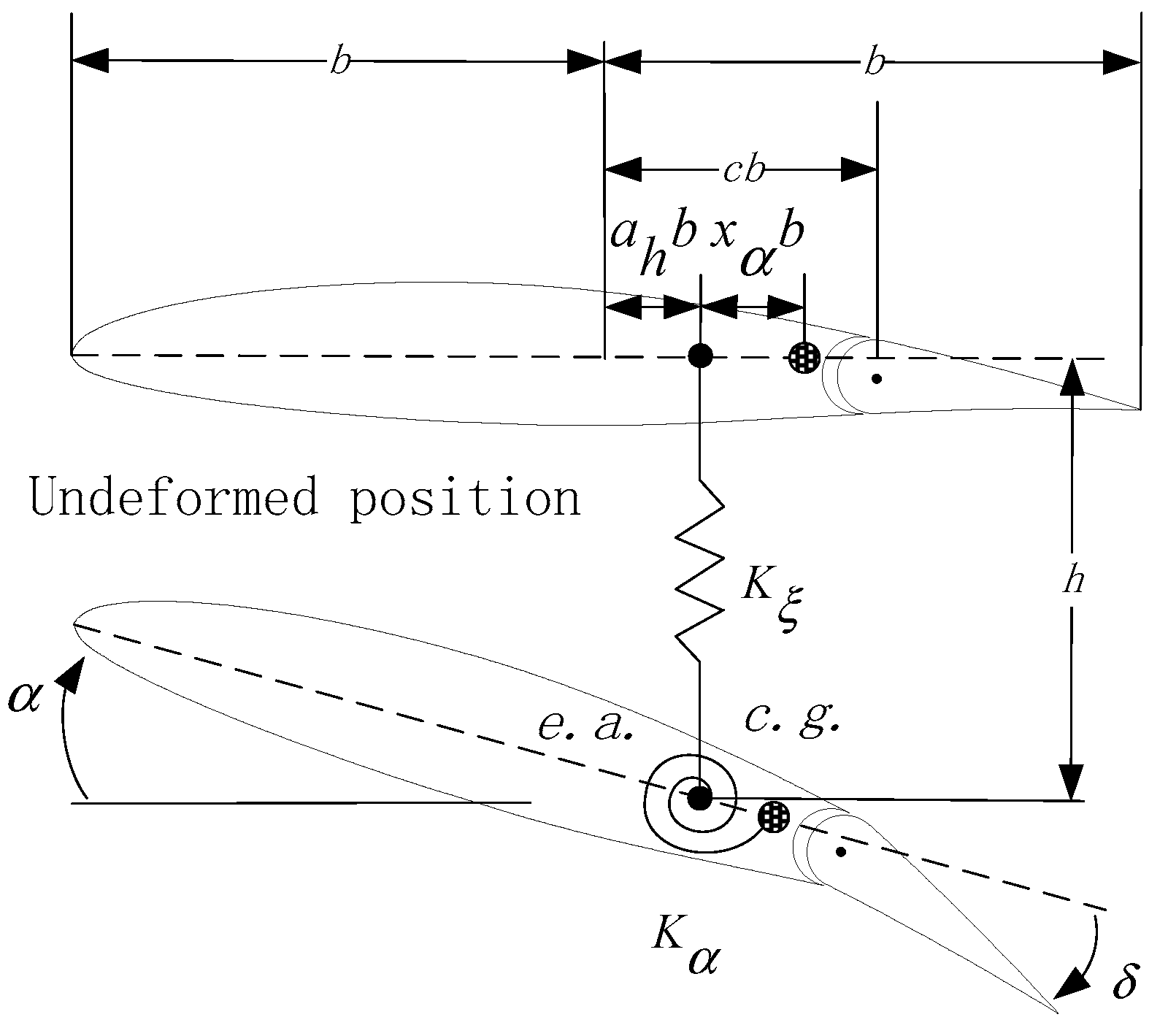
In this work, the aeroelastic test case is for a wing typical section, Figure 1. This is modelled as a two-dimensional symmetric airfoil section and the structural motion is characterized by two degrees of freedom: the plunge, is measured at the elastic axis () and is positive downward; and the pitch rotation, , is the rotation of the airfoil section about the elastic axis, positive nose-up. As common in classic aeroelasticity, is the airfoil semi-chord. The elastic axis is located at a distance from the mid-chord, positive when the elastic axis is aft of the mid-chord. The center of gravity () is located at aft of the mid-chord. The aeroelastic model is restrained to the ground through a system of elastic springs, , and dampers, and (omitted in the figure for clarity), acting on both degrees of freedom. The nonlinearity in the stiffness of the elastic springs is modelled in a polynomial form including terms up to fifth order.
Herein, the interest is to analyze the dynamic response of the system induced by an external disturbance. This disturbance is representative of atmospheric turbulence and gusts, which are treated in more detail in Section 3. A flap is mounted at the trailing-edge of the airfoil, at a distance cb aft of the mid-chord, for GLA. The flap deflection, δ, is defined relative to the airfoil chord.
It is assumed that the system has a horizontal equilibrium position at (, , ). The equations of motion governing the dynamics of the two degrees of freedom system are
The coupled system of equations consists of the structural dynamics on the left-hand side and of aerodynamic loads on the right-hand side. The term (in kg) indicates the total mass that undergoes a vertical motion, (in kg·m) is the first moment of inertia about the elastic axis and (in kg·m2) the second moment of inertia about the elastic axis. The lift, (in N/m), is defined positive upward as usual in aerodynamics, whereas the plunge deflection, , is positive downward as conventionally done in aeroelasticity. Hence, the negative sign in front of the lift. The aerodynamic moment, (in N), is taken about the elastic axis.
The airfoil semi-chord, and the uncoupled pitch natural frequency, , are used to rewrite Equation (1) in terms of non-dimensional parameters. In non-dimensional form, the equations become
It is worth noting that the derivative with respect to physical time, , in Equation (1) is replaced by the derivative with respect to non-dimensional time, , in Equation (2). Non-dimensional parameters are defined in Appendix A.
The aerodynamics is for an incompressible two-dimensional flow [20]. The total aerodynamic loads consist of contributions arising from the airfoil motion, the flap deflection and the encounter with a time-varying gust
The generalization of the aerodynamic loads to an arbitrary input time-history is obtained through convolution (or Duhamel integral). For a practical evaluation of the Duhamel integral, an exponential approximation is used for the Wagner and Küssner functions, which describe, respectively, the indicial build-up of the circulatory part of the lift and the lift build-up for the penetration into a sharp-edged gust [21]. This implies that the governing equations—Equation (2)—are a set of integro-differential equations (IDEs) when an expression for the aerodynamic loads is introduced.
State Space Form
The governing equations are a set of IDEs which are difficult to solve with state-of-the-art algorithms, primarily developed for ordinary differential equations (ODEs). The mathematical procedure to convert the set of IDEs into a set of ODEs is based on defining additional variables and equations describing the evolution of the aerodynamics. Following [22], the aeroelastic equations in state space form are rewritten as
where the dependence on non-dimensional time, , is omitted for brevity. In a matrix-vector form
the state space vector is
The function contains the (nonlinear) elastic contributions from the springs and is a nonlinear function of the state vector, The term indicates the control input (rotation of the trailing-edge flap) and denotes the exogenous external disturbance (atmospheric turbulence and gust). The elements of the state space vector through are aerodynamic states and a full derivation is given [22].
3. Atmospheric Turbulence and Gust Models
Models used for the prediction of the aircraft response need to accommodate those events that are perceived as discrete and usually described as gusts, as well as the phenomena described as continuous turbulence [4].
3.1. Discrete Deterministic Gust
The most common model of a discrete deterministic gust, which has evolved over the years from the isolated sharp-edge gust function in the earliest airworthiness requirements, is the “one-minus-cosine” function. Its formulation is
where is the design gust velocity and is the gust gradient distance, that is, the distance over which the gust velocity increases to a maximum value. Airworthiness requirements prescribe a relationship between the design gust velocity and the gust gradient distance.
3.2. Continuous Atmospheric Turbulence
The engineering model of random turbulence at altitude has been developed over many years. It is now widely accepted that it is satisfactory to treat atmospheric turbulence as frozen, homogeneous and isotropic in relatively large patches. The frozen-field assumption, closely allied to Taylor′s hypothesis, is that turbulent velocities do not change during the time of passage of the airplane. This is a valid assumption in most cases. Dryden and von Kármán models are considered adequate engineering models to predict the correlation and spectra, with the weight of experimental evidence favoring the latter.
A commonly used spectrum that matches experimental data is von Kármán model. The power spectral density (PSD, in m2/(s2Hz)) for the vertical direction, , according to the Military Specification MIL-F-8785C [23], is given by
where is the scaled frequency (in rad/m), the turbulence intensity (in m/s), the freestream speed (in m/s) and the turbulence scale length (in m). The turbulence intensity is related to the wind speed at an altitude of 20 ft (6 m) by
Values of wind speed are tabulated based on the turbulence severity: for light turbulence, = 15 kn; for moderate turbulence, = 30 kn; and for severe turbulence, = 45 kn.
Numerical Implementation
A time-domain representation of the external disturbance is required to simulate the non-linear dynamics of a system in the time-domain. Because of the irrational nature of von Kármán spectrum (in the frequency-domain, the power 11/6 is not an integer), there is no exact analytical formulation in the time-domain corresponding to Equation (8).
The approach used in this work consists of the following steps. First, the Fourier transform of a unit variance band-limited white noise signal, , is calculated. This is passed through a filter, , which is defined as the square root of the PSD spectrum in Equation (8). Then, the output signal is calculated, given the filter and the input signal
Finally, the inverse Fourier transform of the output signal, , is performed to obtain the continuous turbulence in the time-domain, , with statistical properties matching von Kármán spectrum.
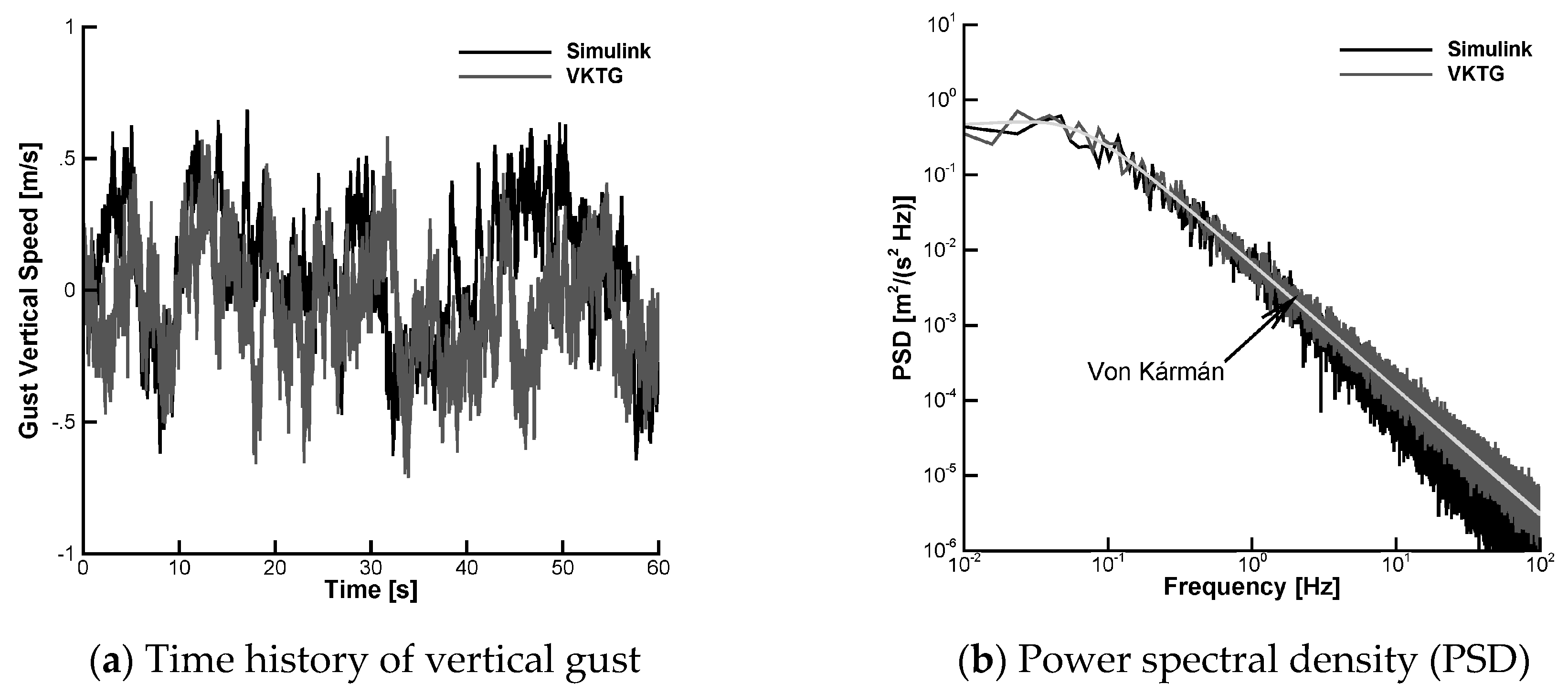
The procedure requires calculating the Fourier transform and its inverse, requiring more computational resources as the time window increases but it was found to be more robust and accurate than other approaches. The method described herein is available in an open-source toolbox (both in MatLAB and Python), which is referred to as the Von Kármán Turbulence Generator (VKTG). The VKTG toolbox implements the mathematical representations of random turbulence defined in the Military Specification MIL-F-8785C and Military Handbook MIL-HDBK-1797, allowing for the dependence of the root mean square turbulent velocity and turbulence length scale on aircraft mission parameters and weather conditions. Figure 2 shows that, at higher frequencies, the PSD of the VKTG model achieves a better agreement with von Kármán spectrum of Equation (8) than the off-the-shelf MATLAB/SIMULINK model. For more information, the reader is invited to refer to Ref. [24] and the on-line documentation (http://daronchlab.com/ (Retrieved 10 August 2018)).
4. Adaptive Feedforward Control
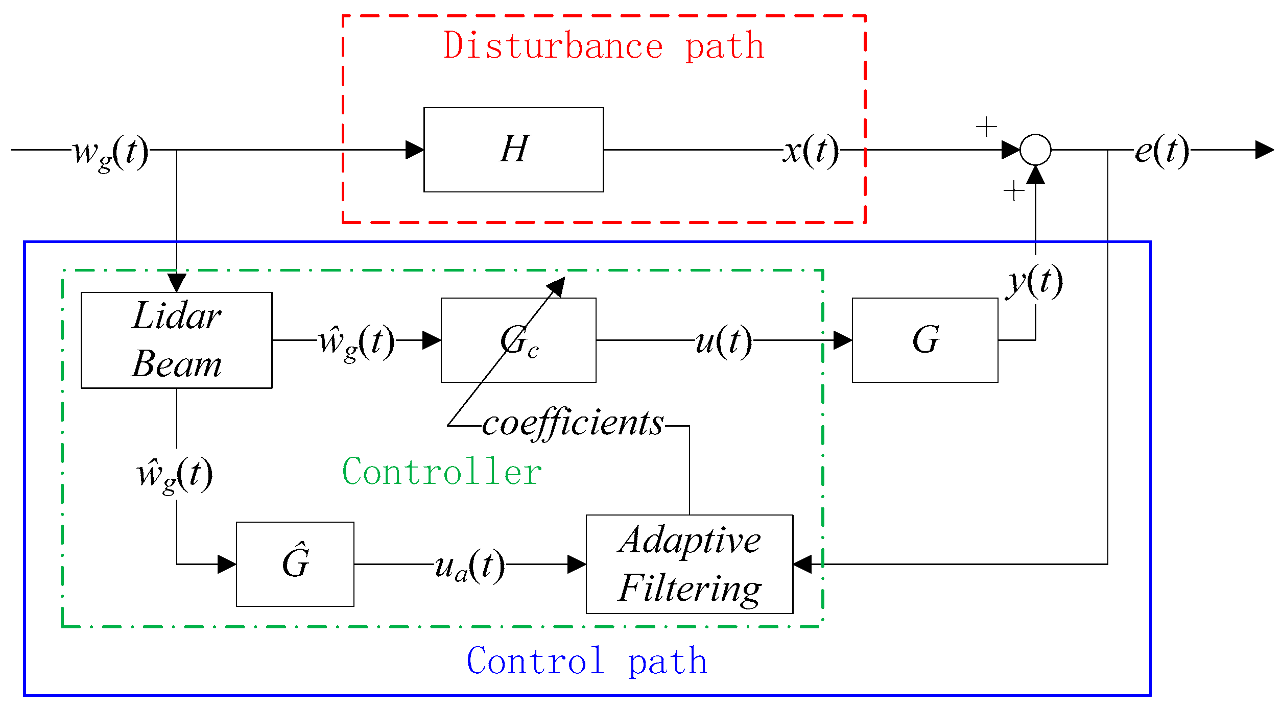
A typical block diagram of an adaptive feedforward control algorithm consists of two channels, Figure 3. The disturbance path includes the transfer function of the physical plant to be controlled, , between the external disturbance, and the system response, . The control path contains the transfer function of the adaptive feedforward controller, , to be designed. The sensed reference signal, , is fed forward to the adaptive controller to generate the control command. The block indicates the transfer function of the physical plant between the control input, and the system response predicted by the model, . The control input to the physical plant is commanded by the controller. Finally, the block with transfer function represents an approximation of . As an input to system , the filter output drives the flap to produce a cancellation force and moment. The error signal, , is the sum of the disturbance path output, and the control path output, .
It is assumed that the wing typical section is equipped with an onboard LIDAR to provide the GLA system with a lead-time reference signal for the vertical gust. The objective of the GLA control is to adjust the weight coefficients of the controller to minimize the error signal . Furthermore, the dynamic characteristics of the actuator driving the rotation of the flap were not accounted. This decision was made based on the experimental observation that the dynamics of the actuator was fast enough, compared to the characteristic times of the aeroelastic plant, to be neglected [22]. Their inclusion is straightforward [25] and their effect would appear within the transfer function .
When there is an exact knowledge of the system transfer functions, and , setting the error to be null
yields the ideal feedforward controller
As this is rarely the case in practice, the transfer functions of the plant are approximated using system identification (SI) methods. Generally, system identification methods seek to create a mathematical relationship between the output response and the input signal. These methods enjoy widespread utilization because the model creation is straightforward. A major drawback is the limited validity of predictions, restricted by the characteristics of the input signal, often referred to as the training signal, used to generate the model in first place [26]. Section 5.3 discusses the choice of the training signal based on a chirp input and evaluates the accuracy of the approximated transfer functions.
Once the system transfer functions and are identified, the block with transfer function is approximated as
The output signal of the block is then calculated
On the disturbance path, the system response is
Substituting Equation (13) into Equation (14) and then substituting from the resulting expression into Equation (15) yields
This relation allows identifying the feedforward controller using a map between and [27]. An adaptive filtering strategy to update the controller gains is adopted to increase the robustness of the weight coefficients of the controller against errors in the measurement of the external disturbance and nonlinear effects in the system response.
4.1. Control Model
The controller is considered as a discrete linear time-invariant system
where indicates the controller transfer operator and is the forward shift operator, . The corresponding transfer function, with , is formulated as
A transfer function for a controller of order is modelled as a sum of coefficients to be determined, , multiplied by an adequate choice of basis functions, . In this work, the basis functions are given by a FIR set
which captures any shape of response up to a frequency limit.
4.2. Exponentially Weighted Recursive Least-Square Algorithm
The calculation of the coefficients of the basis functions, , in Equation (18) is performed using an exponentially weighted recursive least-square algorithm. At the -th time step, , the error between the desired response, and the FIR model output, , is introduced
where is the unknown vector of coefficients (often referred to as tap weight vector) and is the vector containing the output of every basis function. A cost function is then defined as follows
where indicates the total number of time steps and is the forgetting factor.
The adaptive algorithm to calculate the coefficients of the basis functions follows the steps:
- Initialization: parameters are initialized before entering the time iteration loop.is initialized to a column vector of zeros.is the inverse correlation matrix (where in this case).
- Time iteration: the recursive algorithm is repeated at each time step, , for the entire duration of the time vector. For , calculate
The algorithm is sensitive to the choice of the forgetting factor, . In this work, the value is set to 1. The reader is referred to Reference [28] for more details.
5. Results
The aeroelastic solver has previously been validated in many numerical and experimental studies. The reader is invited to refer to References [21,22,29] for further information. Based on previous findings, a non-dimensional time step of 0.05 was deemed sufficient to capture the dynamics of the system.
The aeroelastic parameters in this study model a wind tunnel configuration tested in low speed flow at the University of Liverpool, Figure 4. The experimental model consists of a rigid wing that spans the entire width of the wind tunnel cross-section and is suspended by a system of springs to the tunnel walls. The wing cross-section is based on the NACA0018 airfoil; the semi-chord is m and the pitch natural frequency is rad/s. The aeroelastic parameters are summarized in Table 1 and the procedure for the model updating is discussed in Reference [22]. The last two entries in the table are the cubic and quintic coefficients of the polynomial expansion of the stiffness in the plunge degree of freedom. The values indicate a typical hardening non-linearity.
The wind tunnel test rig exhibited an interesting non-linear dynamic behavior, characterized by the occurrence of sub-critical limit cycle oscillations (LCOs). From a control standpoint, it represents a challenging test case to demonstrate the control and suppression of gust-induced aeroelastic vibrations and LCOs.
5.1. Frequency-Domain Analysis
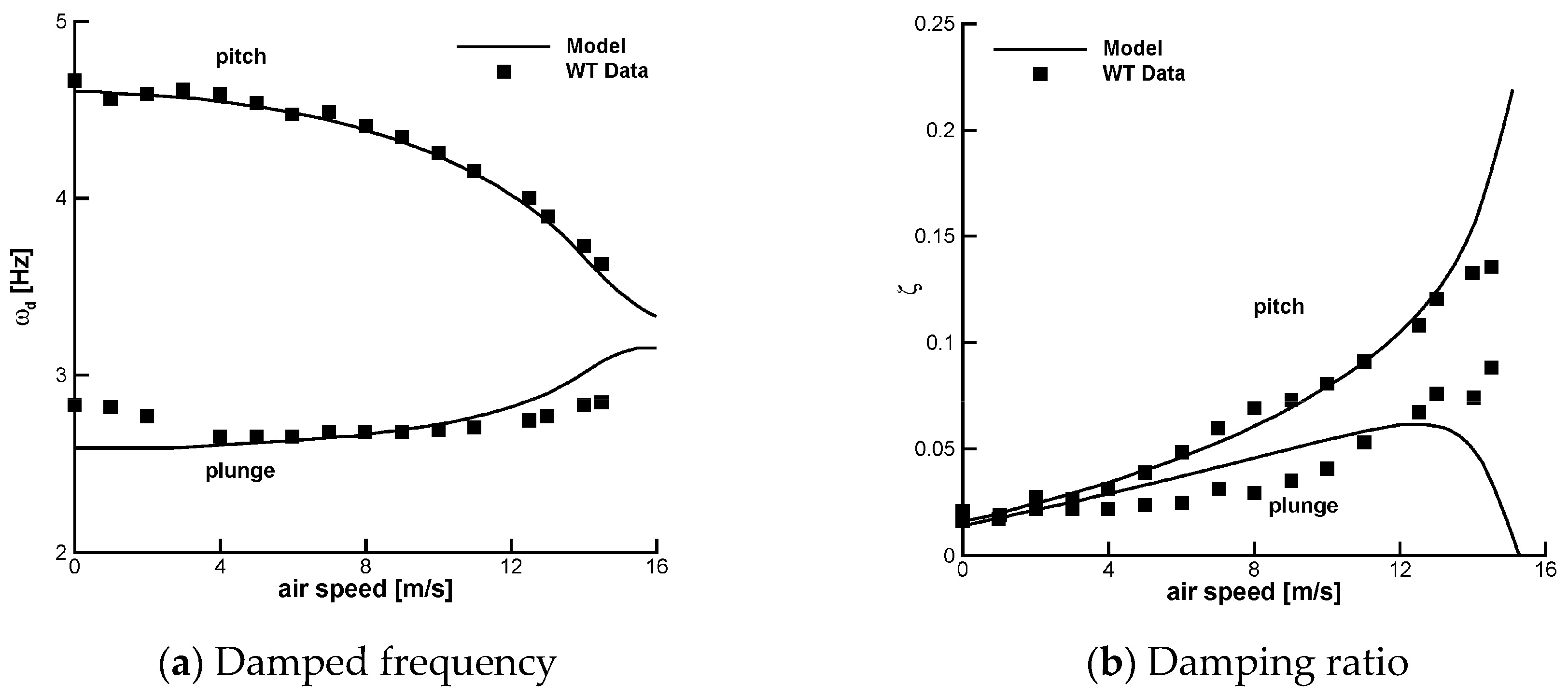
First, the aeroelastic stability is analyzed. Figure 5 shows the damped frequency and damping ratio for varying freestream speed. The solid line in figure is from numerical predictions that were obtained solving an eigenvalue problem of the linearized aeroelastic model. Two sets of experimental data, labelled in figure by “WT Data”, are available: one set resulting from control surface excitation and the other from shaker excitation of the plunge degree of freedom. At intermediate speeds, predictions of damped frequency agree well with measurements. A reason for the agreement degrading at lower speed and close to the flutter speed is the complication in conducting the experiments. At lower speeds, the shaker excitation is used to excite the modes, which in turn may affect the free vibrations of the test rig. Close to flutter, a difficulty is the coalescence of the pitch and plunge frequencies. A reasonable agreement is observed for the aeroelastic damping ratio. Simulations predict a flutter speed of m/s.
5.2. Time-Domain Analysis
The hardening nonlinearity in the plunge degree of freedom, Table 1, was found to significantly affect the dynamics of the system. The aeroelastic system exhibits subcritical LCOs and the amplitude and frequency of LCOs were found in good agreement between measurements and predictions. One example is in Figure 6 where the response to an initial perturbation in angle of attack is simulated at two subcritical speeds (8 and 13 m/s). The onset of LCOs is at a speed of 12.871 m/s. The interest in this work is focused at testing the control strategy of Section 4 at a speed = 8 m/s below the onset point of LCOs.
5.3. Model Identification
The system transfer function, G, is identified by post-processing the input-output relationship. The input, which describes the time evolution of the trailing-edge flap, is a chirp signal defined as
where is a constant value and is the amplitude of the sinusoidal motion. The frequency of the sinusoidal motion, , varies linearly in time
and covers the frequency range [, ] over the total simulation time, . The frequency range is chosen to adequately excite the system over the desired frequency range.
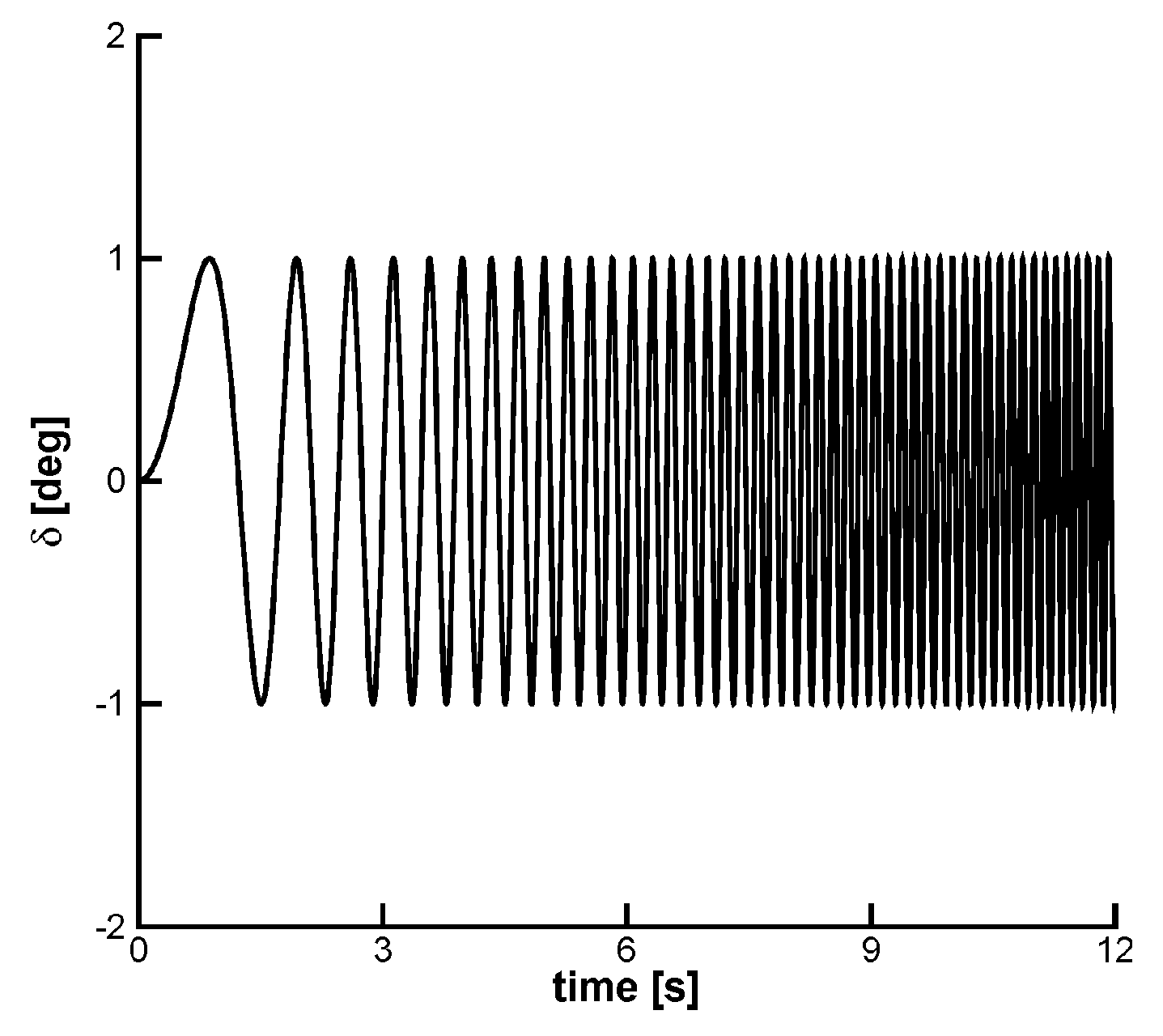
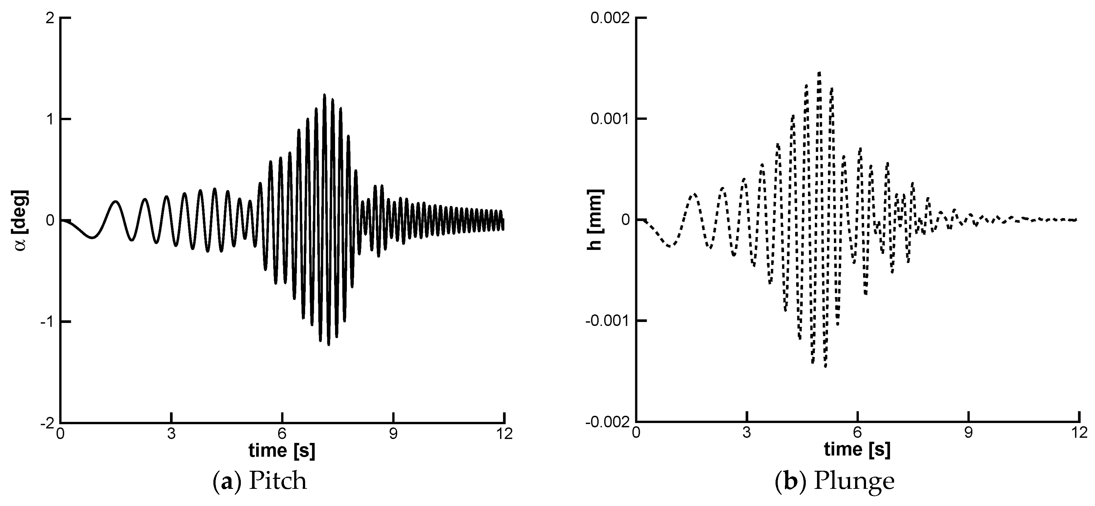
In this work, the parameters of the chirp signal were set to = 0.0° and = 1.0°. The aeroelastic model has two dominant natural frequencies at 2.646 Hz ( = 16.629 rad/s, plunge) and 4.466 Hz ( = 28.061 rad/s, pitch). For increasing dynamic pressure, the pitch and plunge frequencies tend to coalesce, Figure 5 and so the frequency range covered by the chirp signal was chosen between = 0.01 Hz and = 8.0 Hz. The input signal employed for the model identification is illustrated in Figure 7. The aeroelastic response induced by the control surface is shown in Figure 8. The resonant behavior in both degrees of freedom confirms the adequateness of the chosen frequency range.
A SISO model is considered in this exploratory work. The pitch degree of freedom is taken as the measured output, whereas the plunge is assumed unmeasurable. The transfer function, , between the control effector and the pitch response is identified using the prediction error minimization algorithm available in MATLAB. A preliminary study was carried out to ensure independence from the number of zeros and poles used in constructing the transfer function. It was found that six zeros and seven poles, which are listed in Table 2, provide a good approximation of the aeroelastic system composed of 12 states in total. The real part of all poles is negative and the resulting transfer function is therefore stable. As confirmed in Figure 9, the identified transfer function (with six zeros and seven poles) is identical to the transfer function that relates the Laplace transform of the system output to the Laplace transform of the (chirp) input.
5.4. Control for Gust Loads Alleviation
5.4.1. Discrete Deterministic Gust
First, the search for the worst-case-gust was carried out for the “one-minus-cosine” family considering a range of the gust gradient distance, [10,200]. The search, which is an inexpensive process here for the small size of the numerical model, employed a standard Kriging interpolation as response surface method [30]. The worst-case-gust was identified to have a gust gradient distance = 20. The gust intensity was set to a constant value, = 0.1.
Then, the aeroelastic response caused by the worst-case-gust encounter was simulated with and without the adaptive feedforward controller. The comparison is reported in Figure 10. For the pitch, the response with control reveals a significant reduction in the peak-to-peak rotation during and immediately after the interaction with the gust. A reduction of the peak-to-peak rotation up to 50% is recorded. As the gust moves away from the surface of the wing typical section, the improvement in the loads alleviation vanishes because the effective reference input for the control path is null. For the plunge, there is no improvement in the response with control compared to the aeroelastic response without control. This is not unexpected because the controller is a SISO system, with the pitch rotation being the sole measurable quantity for the GLA.
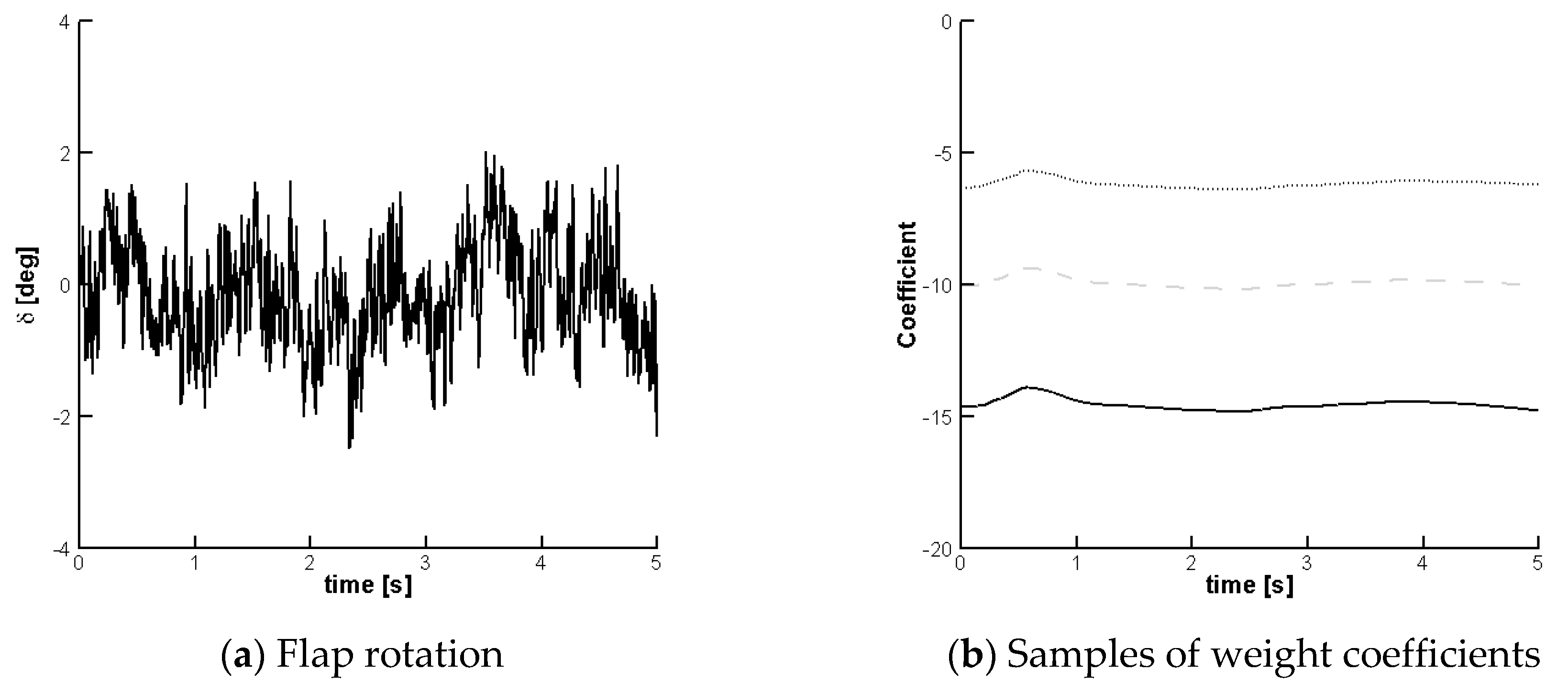
Figure 11 shows the required control action for GLA and a sample of three weight coefficients of the controller. The trailing-edge flap is commanded during the gust encounter, whereas it is unactuated as the gust perturbation moves away from the wing typical section. As the gust propagates along the airfoil, the pitch rotation increases, as shown in Figure 10a. To counter the increasing pitch rotation, the control strategy commands the trailing-edge flap down, that is, a positive control input as shown in Figure 11. This control action has two effects. First, the lift increases, increasing in turn the vertical plunge deflection which is negative, see Figure 10b, according to the sign convention of Section 2. Second, deflecting the flap moves the center of pressure downstream aft of the elastic axis and the increased lift causes a pitch-down rotation. This highlights the capability of the controller to exploit structural flexibility effects to reduce gust-induced aeroelastic vibrations. It is also worth noting that the flap rotation and the angular speed meet fully physical limitations of the experimental test rig: the maximum allowed rotation is ±7° and the speed is limited to 15 Hz. A preliminary study was performed to select the order of the controller. It was found that a controller of order 20 was a good compromise between cost and accuracy. The coefficients of the controller were initially trained for 10,000 time-steps using von Kármán turbulence model.
5.4.2. Continuous Atmospheric Turbulence
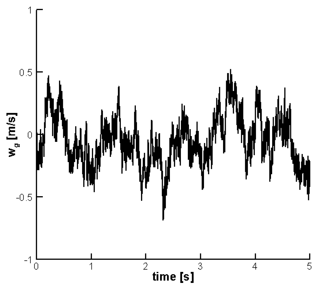
For the random case, atmospheric turbulence was generated with the VKTG toolbox at an altitude = 200 m with the intensity set to “moderate”. The maximum instantaneous gust intensity was set to 10% of the freestream speed, = 8 m/s. The time history of the vertical speed of the turbulence is shown in Figure 12. Figure 13 shows the aeroelastic response with and without control. Similar considerations to those already noted for the discrete gust hold true. The controller is effective at reducing the pitch vibrations throughout the entire duration of the gust encounter.
To quantify the impact of the adaptive feedforward controller for GLA in the presence of atmospheric turbulence, the mean and standard deviation of the pitch and plunge time responses are listed in Table 3. When confronted with the uncontrolled aeroelastic response, the statistics of the pitch rotation are significantly improved by the control action: the mean value is reduced by approximately 80% and the standard deviation by approximately 35%. The increase in the statistics of the plunge is not unexpected, as it was assumed unmeasurable for the purpose of GLA. The trade-off between the reduction in pitch statistics and the increase in plunge statistics is yet in favor of the former.
For the wing typical section, the pitch and plunge are structural modes. The input to the controller is a measure of the pitch degree of freedom, that is, one structural mode. Therefore, it is assumed that the sensor measures solely the torsional mode. An alternative approach to mitigate the effects of a SISO controller for a multi-modal system is to measure a combination of modes. This would be achieved, for the present test case, by placing the sensor at any location other than the elastic axis.
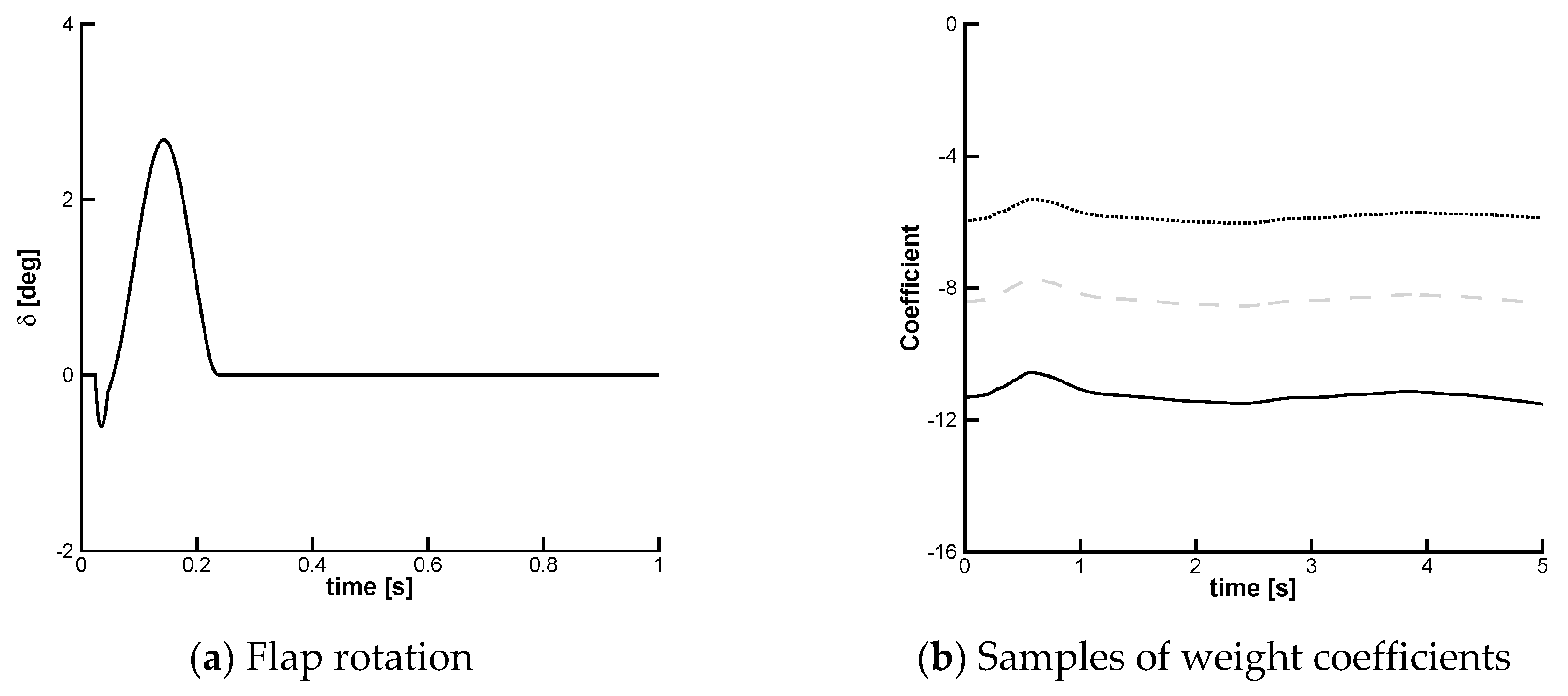
Figure 14 shows the time evolution of the control input to achieve the load alleviation and a sample of three coefficients of the controller. It is worth mentioning that the flap rotation and angular speed meet fully physical limitations of the experimental apparatus (rotation up to ±7° and speed up to 15 Hz).
6. Conclusions
The paper presents the implementation of an adaptive feedforward control strategy to alleviate gust-induced aeroelastic vibrations. The test case is a model problem, consisting of a typical wing section undergoing pitch and plunge motions. The aerodynamics are given by the classic theory of Theodorsen. The stiffness of the springs is modelled in a polynomial form, introducing a nonlinear element to a linear aeroelastic model. The aeroelastic parameters were set to match a wind tunnel test rig and a good comparison between predictions and measurements was found. The effects of structural nonlinearity, for this specific test case, give rise to the appearance of subcritical limit cycle oscillations. The demonstration of the control strategy is performed on a single point near but below the onset of limit cycle oscillations. The control strategy requires an approximate model of the aeroelastic plant and this was created using a system identification method retaining the nonlinear effects on the system response. Although the controller was designed to be a single-input single-output system, the response with control was found effective to reduce the peak-to-peak structural loads during the gust encounters. For a discrete “one-minus-cosine” gust, the peak-to-peak deformations were reduced by about 50% with a negligible effect on the unmeasured structural mode. For a random atmospheric turbulence encounter, which has statistical properties defined by von Kármán spectrum, the feedforward control significantly reduced the mean and amplitude of aeroelastic vibrations.
Directions for future work include:
- the extension of the current work to a multi-input multi-output aeroelastic system;
- an improved treatment of the nonlinearities in creating the approximate system transfer functions;
- the implementation of the controller on an experimental aerial platform which will be flight tested. Initial flight tests have already been conducted to characterize the system dynamic response to forced excitations.
Author Contributions
Conceptualization, G.M.; Methodology, D.A.; Software, validation, formal Analysis and writing-original draft preparation, W.Y.
Funding
This research was funded by the Royal Academy of Engineering (grant numbers: NCRP/1415/51 and ISS1415/7/44) and the Engineering and Physical Sciences Research Council (grant number: EP/P006795/1).
Acknowledgements
Wang acknowledges the financial support received from the China Scholarship Council (CSC) to carry out the research presented in this work at the University of Southampton.
Conflicts of Interest
The authors declare no conflict of interest.
Appendix A
Aeroelastic parameters in dimensional and non-dimensional form and their definitions are reported below.
| airfoil semi-chord | |
| , | lift and pitch moment coefficients |
| , | viscous damping in plunge and pitch, respectively |
| critical damping in plunge, | |
| critical damping in pitch, | |
| , | plunge stiffness and torsional stiffness about elastic axis |
| Non-dimensional plunge stiffness about elastic axis | |
| second moment of inertia of airfoil about elastic axis | |
| airfoil sectional mass | |
| plunge displacement | |
| , | non-linear terms in the state space equations |
| first moment of inertia of airfoil about elastic axis | |
| physical time | |
| airfoil static unbalance, | |
| radius of gyration of airfoil about elastic axis, | |
| freestream velocity | |
| linear flutter speed | |
| reduced velocity, | |
| state space vector | |
| gust vertical velocity | |
| Greek | |
| angle of attack | |
| , | third and fifth order terms of plunge stiffness |
| , | third and fifth order terms of pitch stiffness |
| Trailing-edge flap deflection | |
| , | constants in the approximation of Wagner function |
| , | constants in the approximation of Küssner function |
| Non-dimensional time, | |
| uncoupled plunging mode natural frequency, | |
| uncoupled pitching mode natural frequency about elastic axis, | |
| ratio of | |
| damping ratio in plunge, | |
| damping ratio in pitch, | |
| Non-dimensional displacement in plunge, | |
| mass ratio, | |
| Symbol | |
| differentiation with respect to , |
References
- Dempster, J.B.; Arnold, J.I. Flight Test Evaluation of an Advanced SAS for the B-52 Aircraft. J. Aircr. 1969, 6, 343–348. [Google Scholar]
- Stough, H.P.; Martzaklis, K.S. Progress in the Development of Weather Information Systems for the Cockpit; SAE 2002-01-1520; U.S. Government: Washington, DC, USA, 2002. Available online: https://pdfs.semanticscholar.org/1fae/9889649b575db3eae5d2a754aa936401bf45.pdf (accessed on 9 August 2018).
- Honeywell International Inc. Anon. IntuVue® RDR-4000 3D Weather Radar Systems 2016; Technical White Paper; Honeywell International Inc.: Morris Plains, NJ, USA, 2016. [Google Scholar]
- Tantaroudas, N.D.; Da Ronch, A. Nonlinear reduced order aeroservoelastic analysis of very flexible aircraft. In Advanced UAV Aerodynamics, Flight Stability and Control: Novel Concepts, Theory and Applications; Marques, P., Da Ronch, A., Eds.; Wiley-Blackwell: Chichester, UK, 2017; pp. 143–179. ISBN 978-1-118-92868-4. [Google Scholar]
- Karpel, M. Design for Active Flutter Suppression and Gust Alleviation Using State-Space Aeroelastic Modeling. J. Aircr. 1982, 19, 221–227. [Google Scholar] [CrossRef]
- Regan, C.D.; Jutte, C.V. Survey of Applications of Active Control Technology for Gust Alleviation and New Challenges for Lighter-Weight Aircraft; NASA TM-216008; NASA: Washington, DC, USA, 2012.
- Gangsaas, D.; Ly, U.; Norman, D.C. Practical Gust Load Alleviation and Flutter Suppression Control Laws Based on a LQG Methodology. In Proceedings of the 19th Aerospace Sciences Meeting, Saint Louis, MO, USA, 12–15 January 1981. [Google Scholar]
- Zhou, Q.; Li, D.; Da Ronch, A.; Chen, G.; Li, Y. Computational Fluid Dynamics-Based Transonic Flutter Suppression with Control Delay. J. Fluid. Struct. 2016, 66, 183–206. [Google Scholar] [CrossRef]
- Brosilow, C.; Joseph, B. Techniques of Model-Based Control; Prentice Hall: Saddle River, NJ, USA, 2002; p. 222. [Google Scholar]
- Hahn, K.U.; Schwarz, C. Alleviation of Atmospheric Flow Disturbance Effects on Aircraft Response. In Proceedings of the 26th Congress of the International Council of the Aeronautical Sciences, Anchorage, AK, USA, 14–19 September 2008. [Google Scholar]
- Soreide, D.; Bogue, R.K.; Ehernberger, L.J.; Bagley, H. Coherent Lidar Turbulence Measurement for Gust Load Alleviation; Report No.: NASA Technical Memorandum 104318; Dryden Flight Research Center: Edwards, CA, USA, 1996.
- Zeng, J.; Moulin, B.; De Callafon, R.; Brenner, M. Adaptive Feedforward Control for Gust Load Alleviation. J. Guid. Control Dyn. 2010, 33, 862–872. [Google Scholar] [CrossRef]
- Sleeper, R. Spanwise Measurement of Vertical Components of Atmospheric Turbulence; NASA Report TP-2963; NASA: Washington, DC, USA, 1990.
- Wildschek, A.; Maier, R.; Hoffmann, F. Active Wing Load Alleviation with an Adaptive Feed-Forward Control Algorithm. In Proceedings of the AIAA Guidance, Navigation, and Control Conference and Exhibit, Keystone, CO, USA, 21–24 August 2006. [Google Scholar]
- Wildschek, A.; Bartosiewicz, A.; Mozyrska, D. A Multi-Input Multi-Output Adaptive Feed-Forward Controller for Vibration Alleviation on a Large Blended Wing Body Airliner. J. Sound Vib. 2014, 333, 3859–3880. [Google Scholar] [CrossRef]
- Alama, M.; Hromcikb, M.; Hanisc, T. Active Gust Load Alleviation System for Flexible Aircraft: Mixed Feedforward/Feedback Approach. Aerosp. Sci. Technol. 2015, 41, 122–133. [Google Scholar] [CrossRef]
- Wildschek, A.; Maier, R.; Hahn, K.U.; Leißling, D.; Preß, M.; Zach, A. Flight Test with an Adaptive Feed-Forward Controller for Alleviation of Turbulence Excited Wing Bending Vibrations. In Proceedings of the AIAA Guidance, Navigation, and Control Conference, Chicago, IL, USA, 10–13 August 2009. [Google Scholar]
- Ghandchi Tehrani, M.; Da Ronch, A. Gust Load Alleviation Using Nonlinear Feedforward Control. In Proceedings of the EURODYN 2014: IX International Conference on Structural Dynamics, Porto, Portugal, 30 June 2014. [Google Scholar]
- Wang, Y.; Li, F.; Da Ronch, A. Adaptive Feedforward Control Design for Gust Loads Alleviation of Highly Flexible Aircraft. In Proceedings of the AIAA Atmospheric Flight Mechanics Conference, Dallas, TX, USA, 22–26 June 2015. [Google Scholar]
- Theodorsen, T. General Theory of Aerodynamic Instability and the Mechanism of Flutter; Report No.: NACA Report Nr. 496; NACA Langley Research Center: Hampton, VA, USA, 1935. [Google Scholar]
- Da Ronch, A.; Badcock, K.J.; Wang, Y.; Wynn, A.; Palacios, R.N. Nonlinear Model Reduction for Flexible Aircraft Control Design. In Proceedings of the AIAA Atmospheric Flight Mechanics Conference, Minneapolis, MN, USA, 13–16 August 2012. [Google Scholar]
- Jiffri, S.; Fichera, S.; Mottershead, J.E.; Da Ronch, A. Experimental nonlinear control for flutter suppression in a nonlinear aeroelastic system. J. Guid. Control Dyn. 2017, 40, 1925–1938. [Google Scholar] [CrossRef]
- Moorhouse, D.J.; Woodcock, R.J. Background Information and User Guide for MIL-F-8785C, Military Specification-Flying Qualities of Piloted Airplanes; DTIC Document; DTIC: Fort Belvoir, VA, USA, 1982. [Google Scholar]
- Gianfrancesco, M. Functional Modelling and Design of Energy Harvesters for Slender Wing Structures. Master’s Thesis, University of Southampton, Southampton, UK, 2014. [Google Scholar]
- Zhao, Y.; Yue, C.; Hu, H. Gust Load Alleviation on a Large Transport Airplane. J. Aircr. 2016, 53, 1932–1946. [Google Scholar] [CrossRef]
- Da Ronch, A.; Badcock, K.J.; Khrabrov, A.; Ghoreyshi, M.; Cummings, R. Modeling of Unsteady Aerodynamic Loads. In Proceedings of the AIAA Atmospheric Flight Mechanics Conference, Portland, OR, USA, 8–11 August 2011. [Google Scholar]
- Wang, Y.; Da Ronch, A.; Ghandchi Tehrani, M.; Li, F. Adaptive Feedforward Control Design for Gust Loads Alleviation and LCO Suppression. In Proceedings of the 29th Congress of the International Council of the Aeronautical Sciences, St. Petersburg, Russia, 7–12 September 2014. [Google Scholar]
- Haykin, S. Adaptive Filter Theory, 3rd ed.; Prentice Hall Information and System Science Series; Prentice Hall: Englewood Cliffs, NJ, USA, 2001; pp. 566–569. [Google Scholar]
- Papatheou, E.; Tantaroudas, N.D.; Da Ronch, A.; Cooper, J.E.; Mottershead, J.E. Active Control for Flutter Suppression: An Experimental Investigation. In Proceedings of the International Forum on Aeroelasticity and Structural Dynamics, Bristol, UK, 24–27 June 2013. [Google Scholar]
- Da Ronch, A.; Ghoreyshi, M.; Badcock, K.J. On the Generation of Flight Dynamics Aerodynamic Tables by Computational Fluid Dynamics. Prog. Aerosp. Sci. 2011, 47, 597–620. [Google Scholar] [CrossRef]
Figure 1.
Schematic of an airfoil section with trailing-edge flap; the wind velocity is to the right and horizontal; and denote, respectively, the elastic axis and the center of gravity.
Figure 1.
Schematic of an airfoil section with trailing-edge flap; the wind velocity is to the right and horizontal; and denote, respectively, the elastic axis and the center of gravity.

Figure 2.
Random vertical gust intensity using the Von Kármán spectral representation (Military Specification: MIL-F-8785C; flight speed: = 280 m/s; altitude: = 10,000 m; and turbulence intensity: “light 10−2”; the terms “Simulink” and “VKTG” denote, respectively, the Von Kármán Wind Turbulence Model block of MATLAB and the present Von Kármán Turbulence Generator implementation.).

Figure 3.
Block diagram of an adaptive feedforward control algorithm.

Figure 4.
Experimental test rig of the typical wing section [22].
Figure 4.
Experimental test rig of the typical wing section [22].
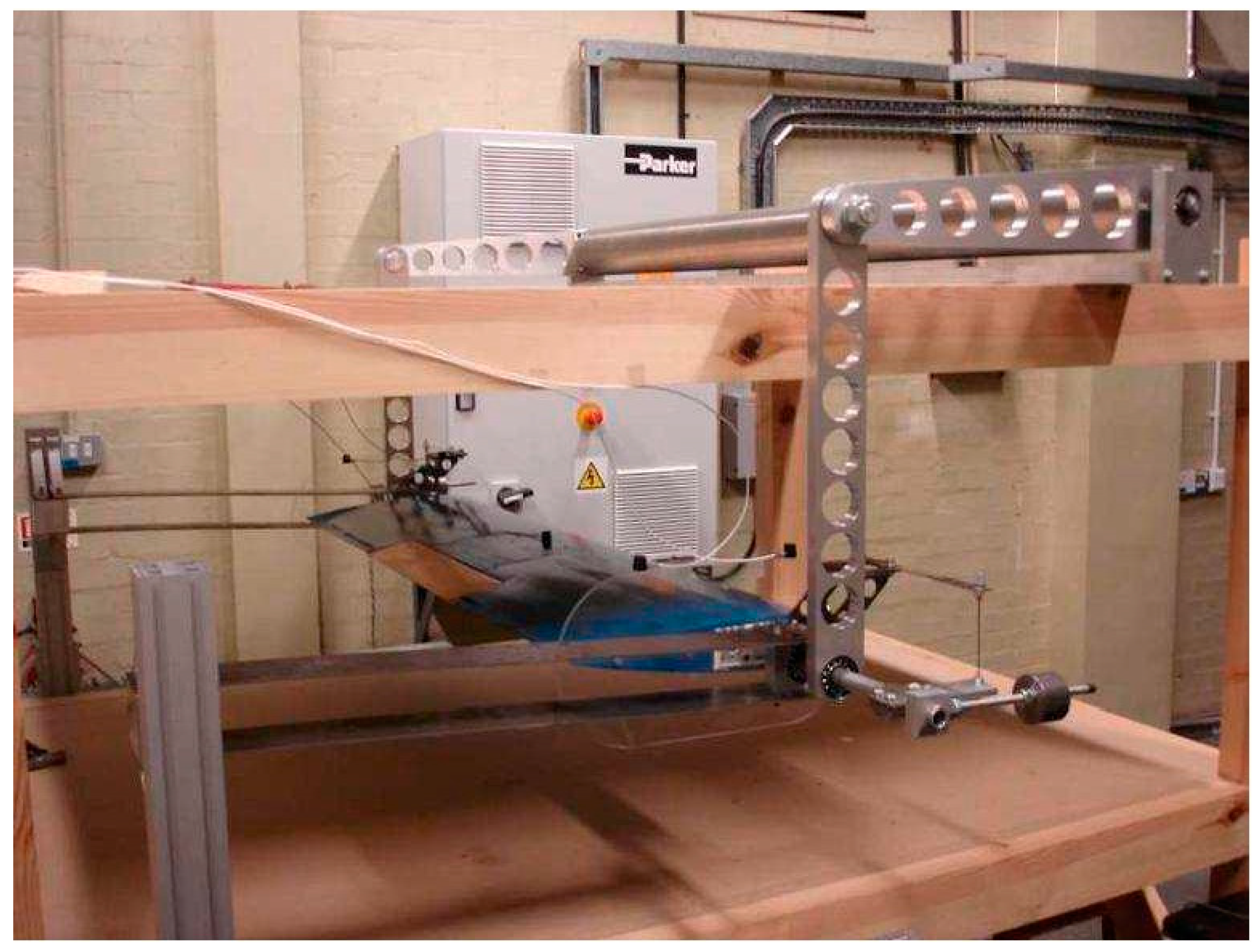
Figure 5.
Dependency of damped frequency, and damping ratio, , with freestream speed; aeroelastic parameters from Table 1 ( = 0.175 m and = 28.061 rad/s); flutter speed predicted at 15.28 m/s.
Figure 5.
Dependency of damped frequency, and damping ratio, , with freestream speed; aeroelastic parameters from Table 1 ( = 0.175 m and = 28.061 rad/s); flutter speed predicted at 15.28 m/s.

Figure 6.
Time-domain response to an initial perturbation in angle of attack ( = 6° at two speeds below the flutter speed, predicted at = 15.28 m/s.
Figure 6.
Time-domain response to an initial perturbation in angle of attack ( = 6° at two speeds below the flutter speed, predicted at = 15.28 m/s.
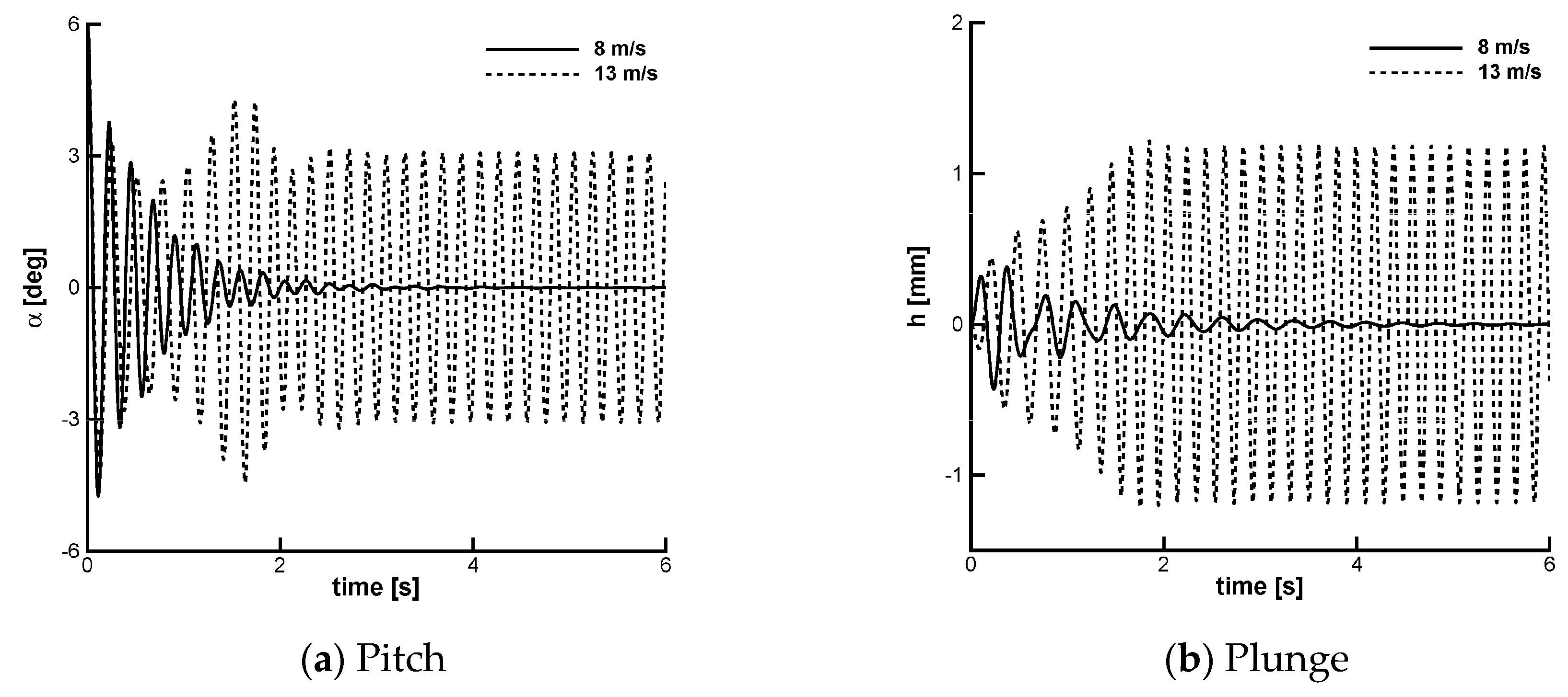
Figure 7.
Chirp input signal of the trailing-edge flap used for the identification of the aeroelastic model ( = 8 m/s, = 0.0°, = 1.0°, = 0.01 Hz and = 8.0 Hz).
Figure 7.
Chirp input signal of the trailing-edge flap used for the identification of the aeroelastic model ( = 8 m/s, = 0.0°, = 1.0°, = 0.01 Hz and = 8.0 Hz).

Figure 8.
Time-domain aeroelastic response to the chirp input signal of Figure 7.
Figure 8.
Time-domain aeroelastic response to the chirp input signal of Figure 7.

Figure 9.
Bode plots of system time-response to a chirp input and the identified transfer function; “Origin” indicates the original model to be identified.
Figure 9.
Bode plots of system time-response to a chirp input and the identified transfer function; “Origin” indicates the original model to be identified.
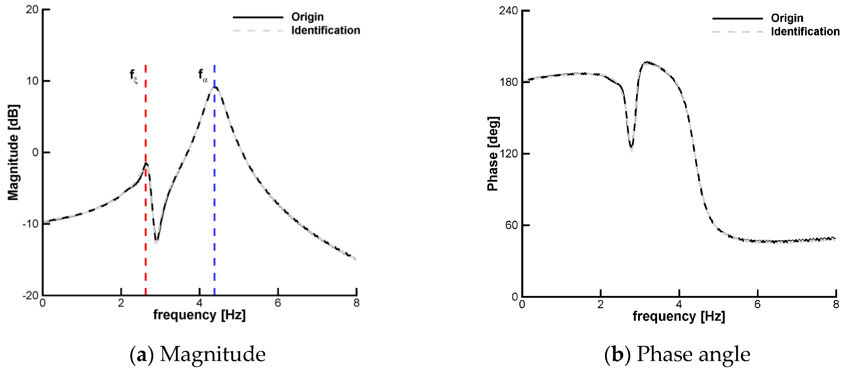
Figure 10.
Aeroelastic response due to the worst-case “one-minus-cosine” gust with and without control ( = 3.5 m, = 0.8 m/s, = 8.0 m/s).
Figure 10.
Aeroelastic response due to the worst-case “one-minus-cosine” gust with and without control ( = 3.5 m, = 0.8 m/s, = 8.0 m/s).
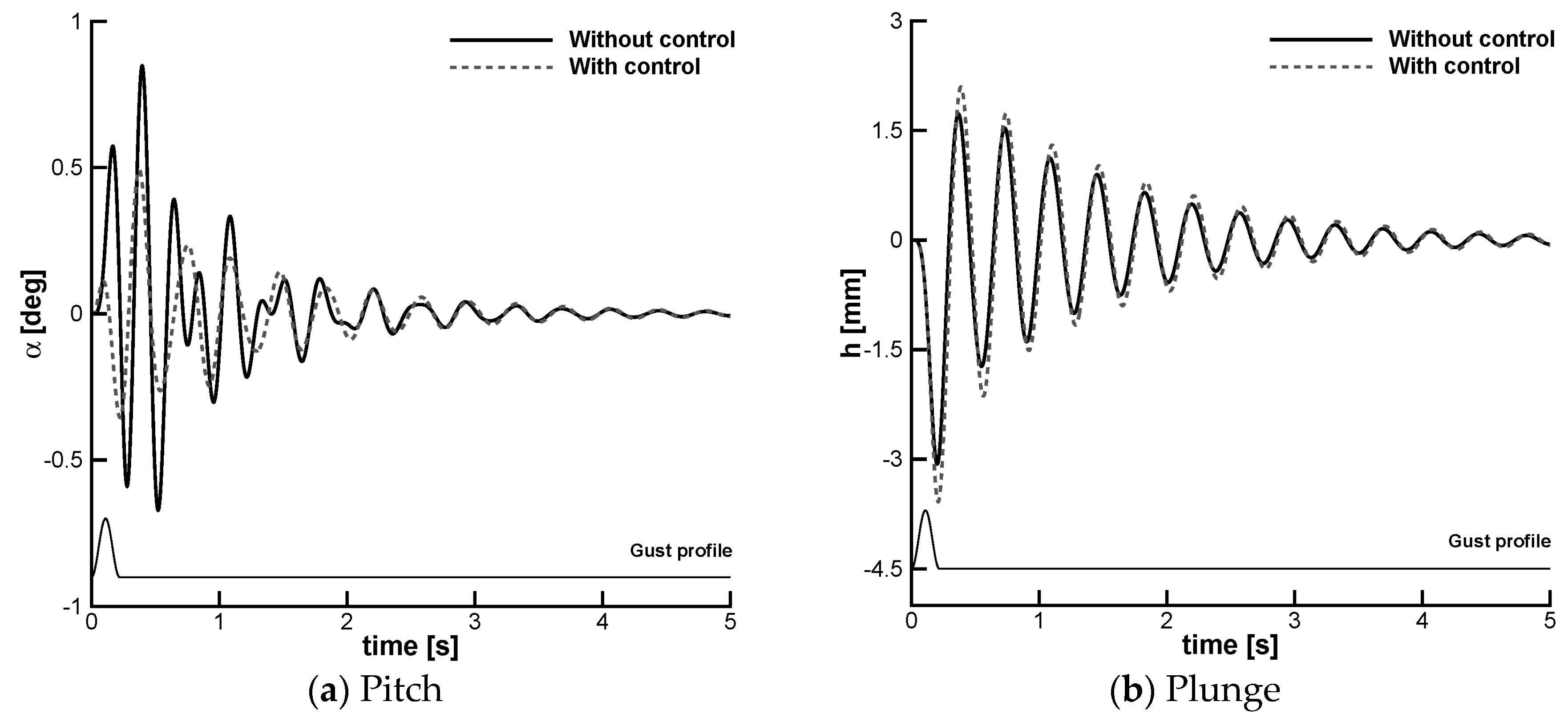
Figure 11.
Aeroelastic response with control corresponding to Figure 10: (a) Commanded rotation of the trailing-edge flap; (b) Three samples (out of 20) of the weight coefficients of the controller.
Figure 11.
Aeroelastic response with control corresponding to Figure 10: (a) Commanded rotation of the trailing-edge flap; (b) Three samples (out of 20) of the weight coefficients of the controller.

Figure 12.
Time history of random atmospheric turbulence with PSD equal to von Kármán spectrum ( = 200 m, intensity: 10−3 “moderate”, = 8 m/s and maximum instantaneous intensity of 0.8 m/s).
Figure 12.
Time history of random atmospheric turbulence with PSD equal to von Kármán spectrum ( = 200 m, intensity: 10−3 “moderate”, = 8 m/s and maximum instantaneous intensity of 0.8 m/s).

Figure 13.
Aeroelastic response due to a random atmospheric turbulence (Figure 12) with and without control.
Figure 13.
Aeroelastic response due to a random atmospheric turbulence (Figure 12) with and without control.
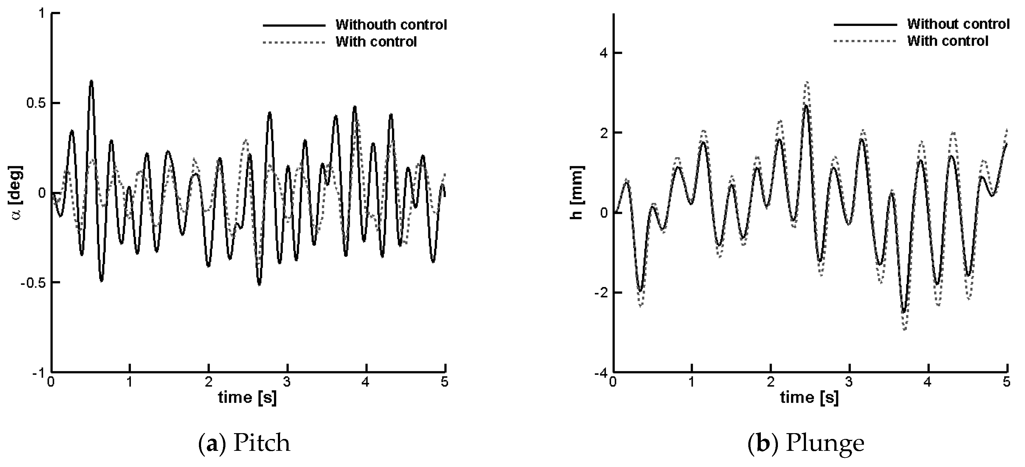
Figure 14.
Aeroelastic response with control corresponding to Figure 13: (a) Commanded rotation of the trailing-edge flap; (b) Three samples (out of 20) of the weight coefficients of the controller.
Figure 14.
Aeroelastic response with control corresponding to Figure 13: (a) Commanded rotation of the trailing-edge flap; (b) Three samples (out of 20) of the weight coefficients of the controller.

Table 1.
Aeroelastic parameters representative of the wind tunnel test rig [22].
Table 1.
Aeroelastic parameters representative of the wind tunnel test rig [22].
| Aeroelastic Parameter | Numerical Value (-) |
|---|---|
| 0.593 | |
| 69.000 | |
| −0.333 | |
| 0.090 | |
| 0.400 | |
| 0.015 | |
| 0.015 | |
| 1741.881 | |
| 638,721.901 |
Table 2.
Identified transfer function of the single-input single-output (SISO) system.
| Zeros (-) | Poles (-) |
|---|---|
| −1.492 ± 1.273i | −0.037 ± 0.604i |
| −0.010 ± 0.394i | −0.018 ± 0.376i |
| −0.523 | −3.982 |
| −0.035 | −0.716 |
| -- | −0.037 |
Table 3.
Statistics of the aeroelastic response induced by atmospheric turbulence.
| Pitch Rotation | Plunge Deflection | |||
|---|---|---|---|---|
| Mean | Standard Deviation | Mean | Standard Deviation | |
| Without control | −0.0389 | 0.2361 | 0.0015 | 0.0060 |
| With control | −0.0085 | 0.1495 | 0.0018 | 0.0072 |
| Improvement (%) | +78.15 | +36.68 | −20.00 | −20.00 |
© 2018 by the authors. Licensee MDPI, Basel, Switzerland. This article is an open access article distributed under the terms and conditions of the Creative Commons Attribution (CC BY) license (http://creativecommons.org/licenses/by/4.0/).
Share and Cite
MDPI and ACS Style
Wang, Y.; Da Ronch, A.; Ghandchi Tehrani, M. Adaptive Feedforward Control for Gust-Induced Aeroelastic Vibrations. Aerospace 2018, 5, 86. https://doi.org/10.3390/aerospace5030086
AMA Style
Wang Y, Da Ronch A, Ghandchi Tehrani M. Adaptive Feedforward Control for Gust-Induced Aeroelastic Vibrations. Aerospace. 2018; 5(3):86. https://doi.org/10.3390/aerospace5030086
Chicago/Turabian StyleWang, Yongzhi, Andrea Da Ronch, and Maryam Ghandchi Tehrani. 2018. "Adaptive Feedforward Control for Gust-Induced Aeroelastic Vibrations" Aerospace 5, no. 3: 86. https://doi.org/10.3390/aerospace5030086
Note that from the first issue of 2016, this journal uses article numbers instead of page numbers. See further details here.