A Hybrid Reduced-Order Model for the Aeroelastic Analysis of Flexible Subsonic Wings—A Parametric Assessment


1
School of Mechanical Engineering, University of Leeds, Leeds LS2 9JT, UK
2
Department of Bioengineering and Aerospace Engineering, Universidad Carlos III de Madrid, 28911 Leganés (Madrid), Spain
*
Author to whom correspondence should be addressed.
Aerospace 2018, 5(3), 76; https://doi.org/10.3390/aerospace5030076
Submission received: 30 April 2018
/
Revised: 25 June 2018
/
Accepted: 9 July 2018
/
Published: 17 July 2018
(This article belongs to the Special Issue Computational Aerodynamic Modeling of Aerospace Vehicles)
Abstract
:A hybrid reduced-order model for the aeroelastic analysis of flexible subsonic wings with arbitrary planform is presented within a generalised quasi-analytical formulation, where a slender beam is considered as the linear structural dynamics model. A modified strip theory is proposed for modelling the unsteady aerodynamics of the wing in incompressible flow, where thin aerofoil theory is corrected by a higher-fidelity model in order to account for three-dimensional effects on both distribution and deficiency of the sectional air load. Given a unit angle of attack, approximate expressions for the lift decay and build-up are then adopted within a linear framework, where the two effects are separately calculated and later combined. Finally, a modal approach is employed to write the generalised equations of motion in state-space form. Numerical results were obtained and critically discussed for the aeroelastic stability analysis of a uniform rectangular wing, with respect to the relevant aerodynamic and structural parameters. The proposed hybrid model provides sound theoretical insights and is well suited as an efficient parametric reduced-order aeroelastic tool for the preliminary multidisciplinary design and optimisation of flexible wings in the subsonic regime.

1. Introduction
Efficient aeroelastic methods and tools [1] based on reduced complexity are increasingly sought for the preliminary multidisciplinary design and optimisation (MDO) [2,3] of flexible aircraft and unmanned air vehicles (UAV). Smart optimisation strategies and algorithms [4] still rely on effective and robust simulations, where the relevant aeroelastic issues and behaviours [5,6] are parametrically analysed in a large design variables space [7]. Fluid-structure interaction (FSI) [8] models coupling finite element methods (FEM) [9] and computational fluid dynamics (CFD) [10] have increasingly been proposed to enhance accuracy [11,12]. However, these high-fidelity tools are computationally expensive [13,14] and require special care [15,16] to ensure that the correct physics are reproduced in their coupling [17,18], especially at all boundaries and interfaces [19,20]. A large amount of time and efforts is then typically necessary for pre-processing the simulations and post-processing the results, which are key features for a reliable implementation of automated MDO routines [21].
A hybrid reduced-order model (ROM) [22,23,24,25,26] for the aeroelastic analysis of subsonic wings in unsteady incompressible flow is presented here within a generalised quasi-analytical formulation. A modified strip theory (MST) is adopted for the aerodynamic load [27,28], tuned (TST) and standard (SST) strip theories being readily resumed for comparison [29]. Thin aerofoil theory is employed for calculating the unsteady air load around each flexible wing section [30,31,32,33,34,35], where the lift deficiency function is corrected by a high-fidelity model in order to account for downwash effects [36]. First, the spanwise decay [37,38] and time-wise build-up [39,40,41,42,43] of the load are separately calculated for the rigid wing by means of a steady and unsteady simulation using the doublet lattice method (DLM) [44,45], as available in the commercial software Nastran [46]. They are then approximated via nonlinear curve-fitting [47] and re-combined a posteriori for use in the linear framework [48] of the proposed quasi-analytical model. A beam-like linear model is considered for the wing structural dynamics [49] and the principle of virtual work (PVW) [50] is used to derive the equilibrium equations. Ritz’s method [51] is finally employed for solving the latter within a modal approach [52], where shape functions are assumed for the displacement [53]. The resulting hybrid ROM allows for arbitrary distributions of the wing properties, providing continuous deformations and loads [54]. Goland’s wing is analysed first for the sake of a thorough validation [55]. The numerical results for both the divergence speeds and flutter frequency of a uniform rectangular flat wing are then shown and critically discussed with respect to the relevant aero-structural parameters, such as aspect and thickness ratios. Finally, Appendix A presents both steady [56,57,58] and unsteady [59,60] lifting line models which can serve as effective and inherently parametric semi-analytical tools [61].
2. Aeroelastic Problem Formulation
According to the closely-spaced rigid diaphragm assumption [62], a slender wing is considered flexible spanwise only and a beam-like model is then suitably employed [63]. Since the latter can be derived from a plate-like model [64], it may represent a physical ROM in itself where the chordwise dependency of the structural properties is dropped [65], and only the pitch and plunge rigid modes of the aerofoil section are retained to allow wing bending and torsion [66], respectively.
The wing has a chord , semi-span and aspect ratio . The elastic axis (EA, where all loads are acting [67]) is modelled as a Rayleigh beam [68] and drawn by the locus of the shear centre of each chordwise section, with fixed for convenience [51,52], whereas the inertial axis is drawn by the locus of the sectional centre of gravity (CG, where the inertial load is applied [67]). Thus, there results a mass as well as bending and torsion moments of inertia and per unit length, an area moment of inertia and a torsion factor , Young’s and shear elastic modules and are distributed along the span .
With and being the vertical displacement and rotation of the EA, respectively, the wing deformation is given as directly. Neglecting gravity and concentrated loads, the PVW for the arbitrary virtual displacements and then reads:
where is the vertical displacement of the inertial axis, whereas and are the sectional unsteady aerodynamic force (positive upwards) and pitching moment (positive clockwise), respectively. The virtual displacement being arbitrary, the bending and torsion virtual work separate and are integrated by parts twice in order to give the linear system of coupled PDEs for the dynamic aeroelastic equilibrium of wing bending and torsion as:
which are consistently completed by both geometrical and natural boundary conditions as:
Note that this standard problem formulation assumes an isotropic material and holds for swept wings too when a chordwise approach is employed [52,69]; if necessary, lumped masses, dampers or springs may easily be included using Dirac’s delta function centred at their applicable location [27,63]. For a slender composite wing, the anisotropic material exhibits different mechanical characteristics in different directions and the resulting elastic coupling between bending and torsion may then be included using the applicable constitutive law, with a more complex calculation of the structural stiffness but no conceptual changes in the overall aeroelastic problem formulation [51].
Modal Solution Approach
Ritz’s method [51] is employed and the beam displacement is then modally expressed as:
where the functions, and functions are the unknown generalised coordinates relative to the mode shapes for bending deformation and mode shapes for torsion deformation, respectively. All mode shapes shall satisfy the geometrical boundary condition for clamped-free beams [63] and may be either assumed [53] or obtained from FEM eigen-analysis or vibrations tests [70,71]. Unlike plate-like models (which require the clamping of the wing root along its entire chord [64]), beam-like models allow a linear torsion mode.
3. Generalised Aerodynamic Load
Within the modal formulation, the generalised unsteady sectional air load is implicitly given as:
whereas the unsteady lift, pitching moment and rolling moment of the wing are given by:
Provided that the effect of the unsteady downwash is included in the indicial function for the wing load development [72], it can be reasonably assumed that steady effects on the spanwise lift distribution due to the wing-tip vortices and unsteady effects on the chordwise lift build-up due to the travelling wake may be considered separately and eventually assembled in a quasi-steady sense [28]; of course, the slower the wing motion (with respect to the aircraft speed) and the higher the aspect ratio, the more accurate the assumption [73]. MST is hence proposed as a physical ROM [27] for calculating the generalised unsteady aerodynamic load, where the lift distribution and evolution are independently combined a posteriori. Note that MTS holds also for compressible flows around arbitrary wings, as long as the coupling between both three-dimensional and compressible effects remains weak and the appropriate indicial functions are employed for the different types of wing motion [5,48,52,74].
Unsteady Modified Strip Theory
According to thin aerofoil theory for incompressible flow [75], the non-circulatory aerodynamic force and moment of each wing section act at its mid-chord (MC), whereas the circulatory ones act at both its aerodynamic centre (AC, where the pitching moment is independent of the angle of attack [76]) and its control point (CP, where the non-penetration boundary condition for the inviscid flow is imposed and the fluid-structure interaction hence enforced [33]). The AC and CP positions and falling at the first and last quarters of the chord [5], respectively, the sectional unsteady aerodynamic force and pitching moment due to the wing motion read as [30,54]:
where all terms involving the lift derivative are of a circulatory nature, whereas all others are of a non-circulatory nature and include apparent inertia effects. Here, and are the speed and density of the reference airflow, , then and are the instantaneous vertical displacements of AC, MC and CP, respectively, while is the equivalent of Wagner’s indicial-admittance function for the circulatory lift build-up due to a unit step in the angle of attack [30]; additional terms appear in the presence of sweep [69] or ailerons [33] (included by means of Heaviside’s step function [52,77] centered at the applicable location). Due to its own motion, each wing section experiences an effective instantaneous angle of attack induced by the net vertical flow velocity , namely [30,54],
starting from an initial (rest) condition. Adopting the lift-curve slope for a flat aerofoil [78], note that Wagner’s and Theodorsen’s formulations [30,33] represent a physical ROM in itself, where the load contribution from small chordwise deformations is neglected and only the pitch and plunge rigid modes are retained from Peters’ general formulation for a morphing aerofoil [65,79].
Within MST [27], the scaling function is introduced in order to account for the span-wise influence of the wing-tip vortices on the sectional air load [37,38,80] and it is consistently derived from Kutta-Joukowsky’s theorem [81,82] based on the steady lift distribution as:
where is the steady circulation distribution and is Oswald’s efficiency factor [83], which embeds the downwash effect. In fact, MST considers the airflow around each wing section as quasi-independent, whereas TST treats it as fully independent and a global scaling factor is then applied to the wing lift; SST disregards all three-dimensional effects and is obtained for the limit of infinitely slender wings, with Wagner’s function giving the lift-deficiency [30].
When the scaling function is based on lifting line theory (LLT, of which SST is the forcing term [27]; see Appendix A), MST may be regarded as a quasi-unsteady ROM for the unsteady LLT [84,85,86]; yet, the overall tuning concept is completely general [87,88] and such a function may then be derived based on the steady lift distribution obtained from any appropriate source [89,90,91,92,93,94,95,96,97,98], such as the vortex lattice method (VLM) [36], DLM [99], CFD [100] or experiments. In all cases, the proposed correction applies only to the circulatory load development of each wing section, whereas the non-circulatory load has an impulsive nature and remains uncorrected for three-dimensional effects [42,52]. From a theoretical point of view [80], the scaling function depends on both flow conditions and actual wing geometry, which in turn, depends on the total applied load and is not known a priori for flexible aircraft. In the presence of small deformations, the scaling function may be calculated for the undeformed wing only and then consistently used for the deformed wing [27]; furthermore, a unit angle of attack may be assumed without loss of generality when linear aerodynamic methods are used [5]. In the presence of large deformations [101] or in the case of non-planar wings [102], the scaling function would also include the geometrically nonlinear effects of the wing curvature on the local load; thus, the flying wing shape and actual angle of attack shall be considered, especially when nonlinear aerodynamic methods are used. However, note that a database of steady lift distributions may be available from previous aerodynamic design studies and also parametrically approximated in order to boost the overall design process efficiency via multi-fidelity surrogate models [103,104].
The calculated scaling function may then be approximated with Prandtl’s expansion [56] as:
where the coefficients can be obtained via either Fourier integrals or curve-fitting directly [105]; this scaling function would also apply to wind gust loading, regardless of the penetration effect [31]. Contrary to LLT, note that the proposed MST inherently prevents projection of all the structural modes on each of the assumed aerodynamic mode, thus reducing the problem size times [27].
4. Added Aerodynamic States
For two-dimensional unsteady incompressible potential flow, Wagner’s lift-deficiency function accounts for the inflow generated by the travelling wake of a flat aerofoil [30,61]; it may be obtained from Theodorsen’s function [33] and vice versa, due to reciprocal relations [106,107] and analytical continuation in the Laplace domain. For three-dimensional flow, the lift-deficiency function includes the unsteady downwash of the trailed wing-tip vortices [39] and is approximated for computational convenience with a series of exponential terms in the reduced time domain [108] (i.e., a series of rational terms in the reduced frequency domain [109]), namely,
where all coefficients are obtained by best-fitting the reference curve for the specific wing shape with the exact constraint [105], whereas is a reference chord (e.g., the wing root chord). In the case of SST, with and with are commonly used [39]; two approximation terms are also typically sufficient for wings of industrial interest [110] and an added aerodynamic state is hence introduced which evolves according to the linear ODE:
Note that the concept of indicial-admittance function is completely general [5,48,111] and the reference curve may be obtained from any appropriate analytical or numerical source, such as DLM [99], CFD [112,113] or experiments; still, when the lift-deficiency function is based on unsteady LLT (see Appendix A), MST may indeed be regarded as a quasi-unsteady ROM. From a theoretical point of view, the indicial aerodynamic function also depends on both flow conditions and actual wing geometry; therefore, the very same comments and assumptions as for the scaling function of the lift distribution apply. The lift-deficiency function may be calculated for the undeformed wing and then consistently be used for the deformed wing; a unit angle of attack step may be assumed without loss of generality whenever linear aerodynamic methods are used [5]. In fact, a database of lift-deficiency functions may be available from previous flight dynamics studies and parametrically approximated in order to significantly accelerate the overall design process [103,104]. Accounting for the penetration effect [31,35], the very same methodology and considerations would also apply to wind gust loading, due to linearity.
Unsteady Air Load
The generalised unsteady aerodynamic load per unit span now reads in the state space as:
and can also be expanded in terms of the assumed modal base as and , with ; therefore, taking advantage of linear superposition, the modal unsteady air load , , , and the added states , are also eventually found in terms of the generalised coordinates, with each resulting term of strip theory projected onto the mode shapes and , respectively.
5. Analytical Aeroelastic Analysis
By substituting the modal expansions in the PVW, the aeroelastic equilibrium PDEs eventually become a linear system of ODEs for the generalised coordinates, namely [114]:
with generalised structural mass , damping and stiffness matrices, aerodynamic load vector , aerodynamic mass , damping and stiffness matrices, all depending on the wing shape and properties; is the unknown vector of generalised coordinates (including added aerodynamic states), which drives the aeroelastic dynamic response. It is worth noting that a change of variables is always possible, as long as a rigorous transformation matrix can be defined and all aero-structural matrices are then consistently projected onto the new modal base [51,79].
The aeroelastic response and stability analysis of the subsonic wing are then governed by:
respectively, or their equivalent first-order forms [114]:
where , and are the generalised aeroelastic mass, damping and stiffness matrices, which depend parametrically on the aircraft speed. In particular, flutter occurs at the lowest flow speed , hence the real part of at least one of the complex eigenvalues becomes positive (i.e., the aeroelastic dynamic behaviour becomes unstable through a Hopf bifurcation [55,66], where a couple of conjugate eigenvalues cross the imaginary axis and leave the response undamped for unsteady flow), two or more generalised aeroelastic modes coupling at the flutter frequency . Note that real and imaginary parts of the complex eigenvalue are related to the effective modal damping and vibration frequency of the wing [115], respectively, with its natural vibration modes being correctly recovered in the absence of air [51,68]. Finally, the static divergence speed is the lowest flow speed making at least one of the eigenvalues cross the imaginary axis on the real axis, and then, the aeroelastic stiffness matrix and static response become singular [55,66] (i.e., structural and aerodynamic forces do not find a stable equilibrium for steady flow).
6. Numerical Aeroelastic Analysis
The commercial aeroelastic solver Nastran [46] was here used as the full-order model (FOM), following the good practice shown in the chapter, “Dynamic Aeroelastic Response Analysis” of the Aeroelastic Analysis User’s Guide [116]. A beam-like FEM and a lifting-surface DLM were built and coupled via splines interface [117] for transferring both loads and displacements, resulting in the numerical aeroelastic model. Note that the latter needed to be re-generated for each and every case to be parametrically investigated, including pre-processing and post-processing.
The beam was modelled using CBEAM elements and RBE2 rigid elements were added to each finite element node in order to support splining; the node lying at the wing root was then clamped. The aerodynamic lifting surface was aligned with the freestream and modelled as a flat plate divided into an appropriate number of CAERO panels placed along the wing span and chord. The RB2 elements were designed to match the leading and trailing edge of the aerodynamic surface and provide a natural support for splining; in particular, surface splines SPLINE1 were used and the infinite plate spline (IPS) [118] was selected among the available options.
For the natural vibration analysis, shear deformation was neglected and Rayleigh beam theory [68] was used, with PBEAM defining the properties (i.e., inertia and stiffness) of the beam element and SPC1 defining the single-point constraint for the clamped root. The vibration analysis was then performed using Lanczos’ method [119], which was among those available in EIGRL, normalising the modes to unit values of the generalized mass.
For the aerodynamic analysis, the matrix of complex aerodynamic influence coefficients (AIC) [44] was generated (in the physical space) at several reduced frequencies specified in MKAERO1; which includes coupling terms between unsteady wake inflow, vortices downwash, fluid compressibility and apparent inertia, as the DLM is formulated for subsonic potential flow [114]. Load symmetry with respect to the vertical plane was always imposed at the wing root. Well-established guidelines on results accuracy and robustness relate the highest reduced frequency to the number of panels placed along the chord [120]; no additional correction [121] was implemented.
For the steady aerodynamic load analysis and scaling function derivation, a unit angle of attack was specified for the clamped rigid wing in TRIM. Taking advantage of SPLINE2, the strip-wise normal force and pitching moment coefficients (at the strip leading edge) distribution was finally obtained along the wing span using the straightforward MONCNCM.
For the unsteady aerodynamic load analysis and lift-deficiency function derivation, the plunge motion was released to impose a unit step change in the angle of attack. The latter was prescribed as a time-dependent dynamic excitation in TLOAD1, in terms of an enforced velocity motion in SPCD, within the framework of a transient response analysis; the full-time history of the dynamic excitation (i.e., a positive square wave followed by an equal and opposite one) was specified in TABLED1. A very stiff scalar spring element was then defined at the EA root in CELAS2, in order to avoid any significant vertical displacement of the rigid wing resulting from the imposed dynamic excitation; a rigid-body spline SPLINRB was used for interpolating the spring motion and forces. The dynamic excitation is automatically Fourier-transformed and the transient response problem is solved in the frequency domain, based on the frequency range and resolution specified in FREQ1. Fourier inverse transform is then used to obtain the solution back in the time domain, using the time-step interval specified in TSTEP. The wing lift was monitored at the EA root, where the stiff spring was located.
For the static aeroelastic divergence analysis, two different yet still equivalent approaches were adopted: a complex eigenvalue analysis using Lanczos’ block method [119] as defined in EIGC with Mach numbers specified in DIVERG, a dynamic aeroelastic divergence analysis at zero frequency.
For the dynamic aeroelastic divergence analysis, the p-k method [122] as available in FLUTTER was used with a non-iterative frequency-sweeping technique, where the unsteady AIC matrix is first projected onto the modal space and mode-tracking is then performed via the eigenvectors correlation matrix. Note that the p-k method uses only real matrix terms for computing the flutter solution [114], meaning that any imaginary terms in any of the matrices are ignored and the imaginary part of the AIC matrix is added as a real matrix to the viscous damping matrix. Finally, flutter analyses were also performed with two-dimensional aerodynamics (PAERO4 and CAERO4) for direct validation.
7. Results and Discussion
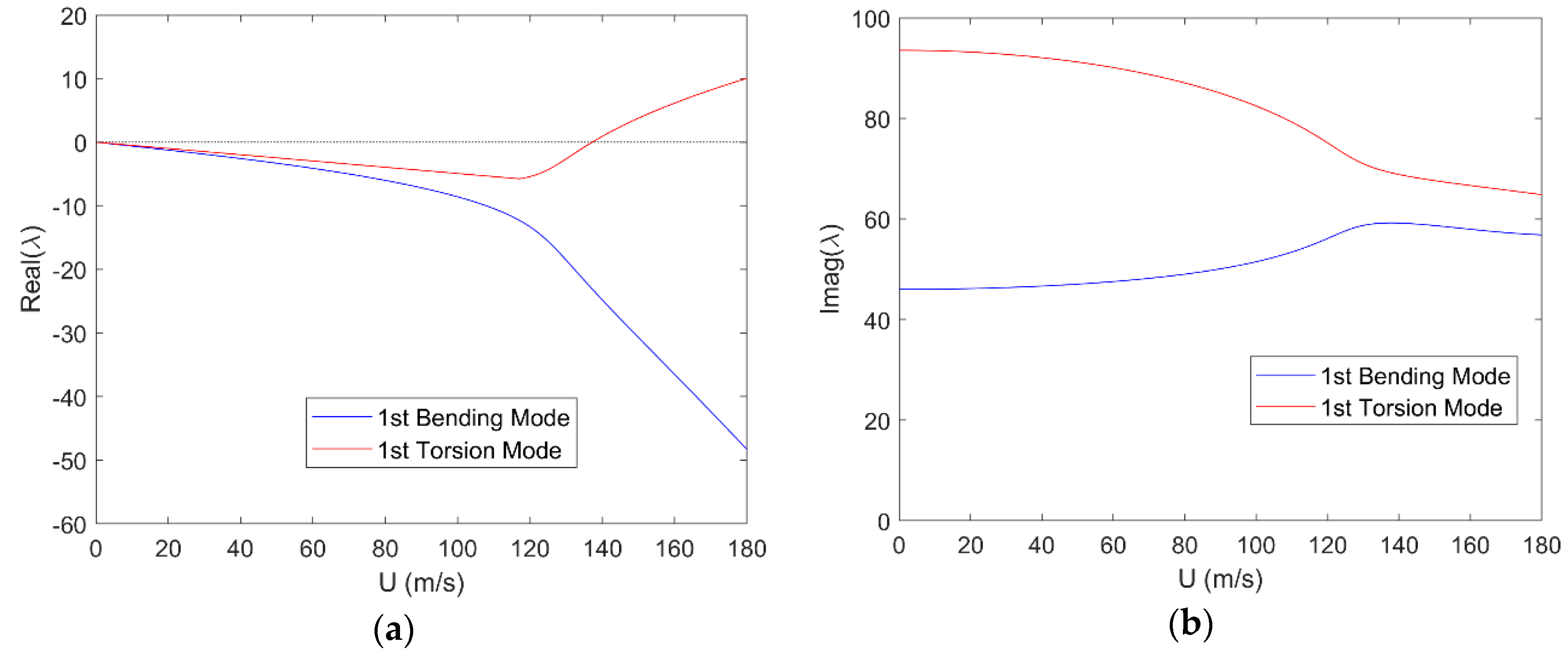
Goland’s wing [123,124] was considered first, since it is widely used as a fundamental reference for validation as well as an ideal prototype for investigating new methods and concepts. It is a flat thin uniform rectangular cantilevered wing with m and m; the wing root is clamped at its elastic axis with stiffness EI = 9,772,200 Pa∙m4 and GJ = 987,600 Pa∙m4 at 33% of the wing chord, while the inertial axis with mass kg/m and kg∙m lays at 43% of the latter. The wing is aligned with the horizontal reference airflow, which is assumed to be incompressible [123]; then the aerodynamic center and control point are consistently at 25% and 75% of the wing chord, respectively. Goland’s wing exhibits the prototypical flutter mechanism coupling its fundamental bending and torsion modes, the uncoupled natural vibration frequencies of which were found at Hz and Hz, respectively, as expected [125]. Figure 1 shows the evolution with the airspeed of the real and imaginary parts of the relative complex eigenvalues calculated by the hybrid ROM, using unsteady SST with Wagner’s function approximation [39] for the aeroelastic stability analysis in a standard atmosphere at sea level ( kg/m3 [126]). Due to the torsion mode becoming unstable and extracting energy from the coupled bending mode, flutter is found at m/s and Hz, which is in excellent agreement with previous results [123,124,125,126,127,128]; then, the flutter Mach number confirms that the incompressible flow was correctly assumed [129]. When using unsteady MST for the aeroelastic stability analysis at about 6100 ft altitude ( kg/m3 [126]), flutter is found at m/s and Hz, which is still in remarkable agreement with the existing results [130]. In this case, five sinusoidal and two exponential terms were respectively employed to approximate the lit distribution and build-up as obtained by Nastran’s DLM [45] with a grid of 48 spanwise and 12 chordwise panels and 14 reduced frequencies in the range , which largely covers the reduced flutter frequency. In all cases, employing the first two bending and torsion modes (correctly found at Hz, Hz, Hz, Hz, also when using Nastran’s FEM [46]) granted convergence of the aeroelastic stability analysis [130].
Following Goland’s concept, a flat rectangular cantilevered wing of uniform material and chord m is now considered; the wing root is still clamped at the elastic axis. Flexural and torsional stiffness of the wing are respectively given by [67]:
for the rectangular cross-section of the beam-like model, where is the section thickness, while the mass and second moments of inertia per unit area read [67]:
where is the material density. Both elastic and inertial axes coincide with the symmetry axis, namely m; m and m for incompressible flow [33].
Neglecting structural damping without loss of generality, divergence speed, flutter speed and flutter frequency are parametrically investigated with respect to both aspect and thickness ratios for a uniform wing, considering kg/m3, Pa and as in previous studies [131]. Nine aeroelastic configurations resulted from combining three aspect and thickness ratios, namely:
ranging from relatively low to relatively high values in order to investigate their physical role and influence on structural dynamic, aerodynamic and aeroelastic behaviours of the flat wing. This is particularly useful in multidisciplinary optimisation studies for preliminary design [7].
7.1. Structural FEM and Aerodynamic DLM for Numerical Simulations
A discrete aeroelastic model was built and used in Nastran for every configuration, based on rigorous convergence studies (not shown) on the aeroelastic results. Table 1 presents the selected number of nodes and elements of the structural FEM along with the number of spanwise and chordwise panels of the aerodynamic DLM. Figure 2 shows structural FEM and aerodynamic DLM arrangements for all wings with , as an example: the wing EA is clamped at the root mid chord, while the RBE2 elements realise the wing torsion and transfer the chordwise pressure loads.
7.2. Natural Vibration Modes
In the case of uniform beams, the exact natural vibration mode shapes and frequencies are well known for both bending and torsion as [51,52]:
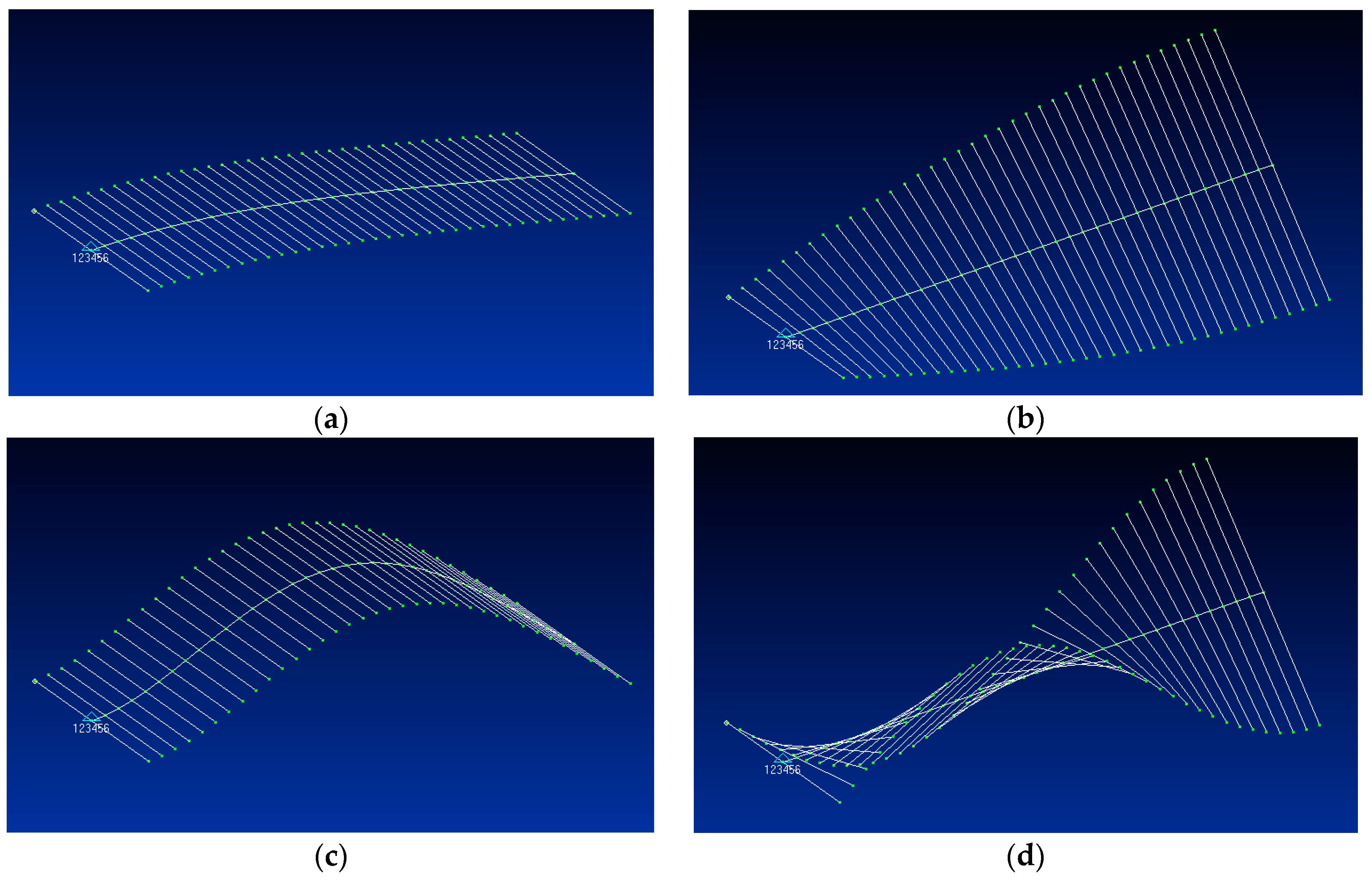
and form the modal base for the analytical model and generalised solutions. Figure 3 shows the first four FEM modes for the wings with , whereas Figure 4 shows the first two bending and torsion exact modes (which hold for all aero-structural configurations). Table 2 shows the typology of both FEM and the exact natural vibration modes, independent of the thickness ratio. The relative natural frequencies do depend on the latter and are shown in Figure 5, where exact agreement is found between numerical and analytical results: this cross-validates both and demonstrates that FOM and ROM are equivalent as far as structural dynamics are concerned.
Note the switch between bending and torsion in the second, third and fourth modes for wings with , since the natural frequency of the bending modes decreases more rapidly than that of the torsion modes with an increase in the wing span.
7.3. Steady and Unsteady Air Load
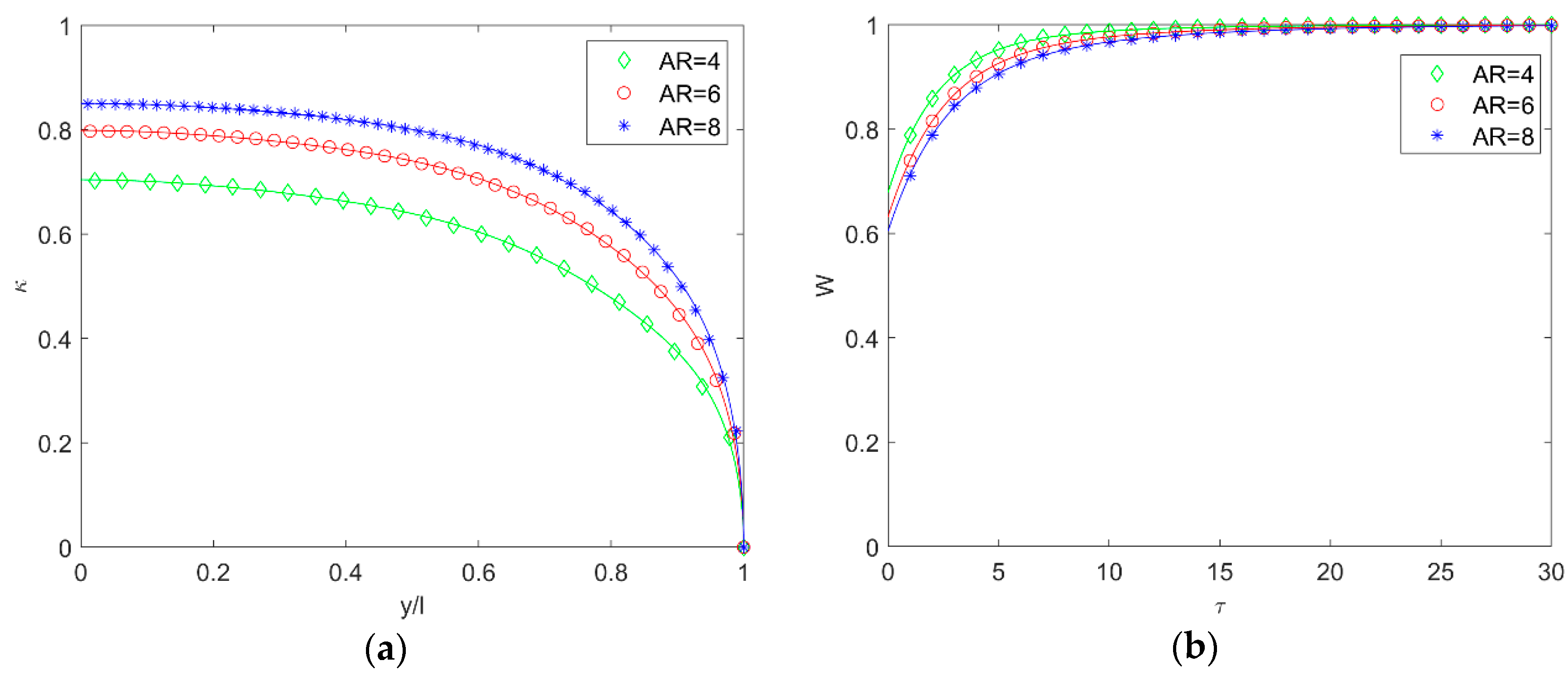
The air load steady distribution and unsteady evolution were calculated by the DLM with a unit angle of attack for the undeformed wings and then approximated to derive the analytical ROM. As the subsonic DLM formulation inherently tends to infinity at the start of the indicial response for the case of incompressible flow [5] (where the exact solution exhibits a Dirac delta), the initial value was then set as the theoretical one for the circulatory contribution (see Appendix A). As shown in Figure 6, the first 5 (odd) sinusoidal terms granted excellent approximation of the (symmetric) normalised lift distribution, whereas 2 exponential terms gave an excellent approximation of the lift-deficiency function due to a unit step in angle of attack; still, the three-dimensional coupling between unsteady wing-tip downwash and wing-wake inflow is only enforced a posteriori in the MST-based ROM.
Note that a parametric database of steady lift distributions and unsteady lift evolutions results from the DLM simulations, which may then analytically be approximated and form an aerodynamic ROM where all curve-fitting coefficients are generally expressed as function of the wing [132].
7.4. Divergence and Flutter Analysis
The dependence of the divergence speed, the flutter speed and frequency on aspect and thickness ratios were then investigated. Figure 7 shows both divergence and flutter speeds as calculated by the aeroelastic models when SST is employed for the unsteady aerodynamics and exact agreement is found between the numerical and analytical results. The same is true for the related flutter frequency and reduced frequency shown in Figure 8, which cross-validate both numerical and analytical results. As further proof of the rigorous validation, note that the results for the divergence speed exactly reproduce the theoretical solutions derived in previous studies [27].
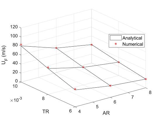
Figure 9 shows both divergence and flutter speeds as calculated by the aeroelastic FOM and ROM when MST and DLM are employed for the unsteady aerodynamics, respectively; excellent agreement is found between numerical and analytical results, with no appreciable difference in the divergence speed. In spite of the DLM compressible formulation, very good agreement is also found for the related flutter frequency and reduced frequency shown in Figure 10, where the discrepancy decreases with increasing the wing aspect ratio as the flow becomes progressively two-dimensional and quasi-steady; thus, coupling between apparent fluid inertia, tip-vortices downwash and wake inflow becomes gradually weaker and differences between FOM and ROM reduce accordingly.
As expected, the SST-based results are more conservative than the MST-based ones, as in the latter case the aerodynamic load builds up but also decays more rapidly towards the wing tip, which is the softer area. Indeed, the resulting bending moment at the wing root is lower in the MST-based cases. Note that both divergence speeds and flutter frequency consistently decrease with decreasing the thickness ratio and increasing the wing aspect ratio; yet, the reduced flutter frequency increases with a decrease in the thickness ratio, as the decrement in the flutter speed is higher than that in the flutter frequency along this dimension of the design variables space. It is also notable that all reduced flutter frequencies fall in the frequency range chosen for the numerical simulations.
The first 5 bending and torsion natural vibration modes granted ROM convergence in all cases. As the flutter phenomenon couples first bending and torsion, the switch between bending and torsion in the third and fourth modes for did not create discontinuity in the results; however, additional simulations showed that hump modes start to develop at higher aspect ratios and lower thickness ratios (i.e., when decreasing the stiffness), as also found in previous works [131].
8. Conclusions
A computationally efficient hybrid ROM for the aeroelastic stability analysis of flexible wings in subsonic flow has been presented. A new modified strip theory was formulated where the unsteady aerodynamic load provided by thin aerofoil theory is corrected by a higher-fidelity model to account for three-dimensional downwash effects on both distribution and build-up of the sectional pressure forces. A slender beam model being coupled for the structural dynamics, the generalised aeroelastic equations were derived by means of the principle of virtual works and then solved using a modal approach that takes full advantage of the implicit projection concept embedded in the aerodynamic scaling function. The proposed FSI ROM allows an arbitrary distribution of the wing’s physical properties and calculates a continuous solution for displacements and loads, which is ideal for parametric optimisation studies over a large design space within aircraft preliminary MDO. Numerical results were obtained using MSC NASTRAN and then compared for both divergence speeds and flutter frequency of a flat rectangular homogeneous wing, given different aspect and thickness ratios. The presented results offer sound insight into the aeroelastic stability of flexible subsonic wings and thus, may be used to assess high-fidelity FOMs. The proposed hybrid modified strip theory demonstrated excellent accuracy at low computational costs with respect to the classic DLM and it is therefore suggested as a general and efficient aerodynamic ROM for the MDO of flexible wings in subsonic flow, especially at the preliminary stage where fast and robust semi-analytical aero-structural tools are highly sought for best computing performance.
Author Contributions
M.B. derived the analytical model and results, whereas R.C. performed the numerical simulations; the authors then wrote the respective parts of the manuscript.
Funding
This research received no external funding.
Conflicts of Interest
The authors declare no conflict of interest.
Nomenclature
| aerodynamic gain coefficient | |
| wing aspect ratio | |
| aerodynamic pole coefficient | |
| section chord | |
| section lift | |
| section lift derivative | |
| wing lift derivative | |
| generalised damping matrix | |
| elliptic integral of the second kind | |
| section Young’s elastic modulus | |
| angular frequency | |
| generalised aerodynamic load vector | |
| section shear elastic modulus | |
| section thickness | |
| section flexural area moments of inertia | |
| section torsional mass moments of inertia | |
| reduced frequency | |
| generalised stiffness matrix | |
| wing semi-span | |
| section aerodynamic force | |
| section mass | |
| section aerodynamic moment | |
| generalised mass matrix | |
| number of expansion terms | |
| time | |
| horizontal air speed | |
| vertical air speed | |
| section vertical displacement | |
| aerodynamic indicial-admittance function | |
| chordwise coordinate | |
| spanwise coordinate | |
| angle of attack | |
| section circulation | |
| flexural generalised coordinate | |
| section flexural displacement | |
| torsional generalised coordinate | |
| section torsional displacement | |
| aerodynamic load-scaling function | |
| eigenvalue | |
| section flexural mass moments of inertia | |
| section torsional mass moments of inertia | |
| Poisson ratio | |
| Oswald’s efficiency factor | |
| reference air density | |
| reduced time | |
| added aerodynamic state | |
| flexural assumed mode shape | |
| torsional assumed mode shapes | |
| generalised coordinates vector | |
| spanwise Glauert angle |
Appendix A. Lifting Line Models for Rectangular Straight Wings
Lifting line theory [56] accounts for the downwash angle induced by the tip vortex and is very powerful for slender straight wings. However, it is generally conservative as the distance between aerodynamic centre lines (where the bound circulation lays) and control points line (where the non-penetration boundary condition for the potential flow is enforced) is neglected when applying Helmholtz’s theorem and Biot-Savart law [36]. Therefore, a correction [57] should be considered in the presence of a small aspect ratio.
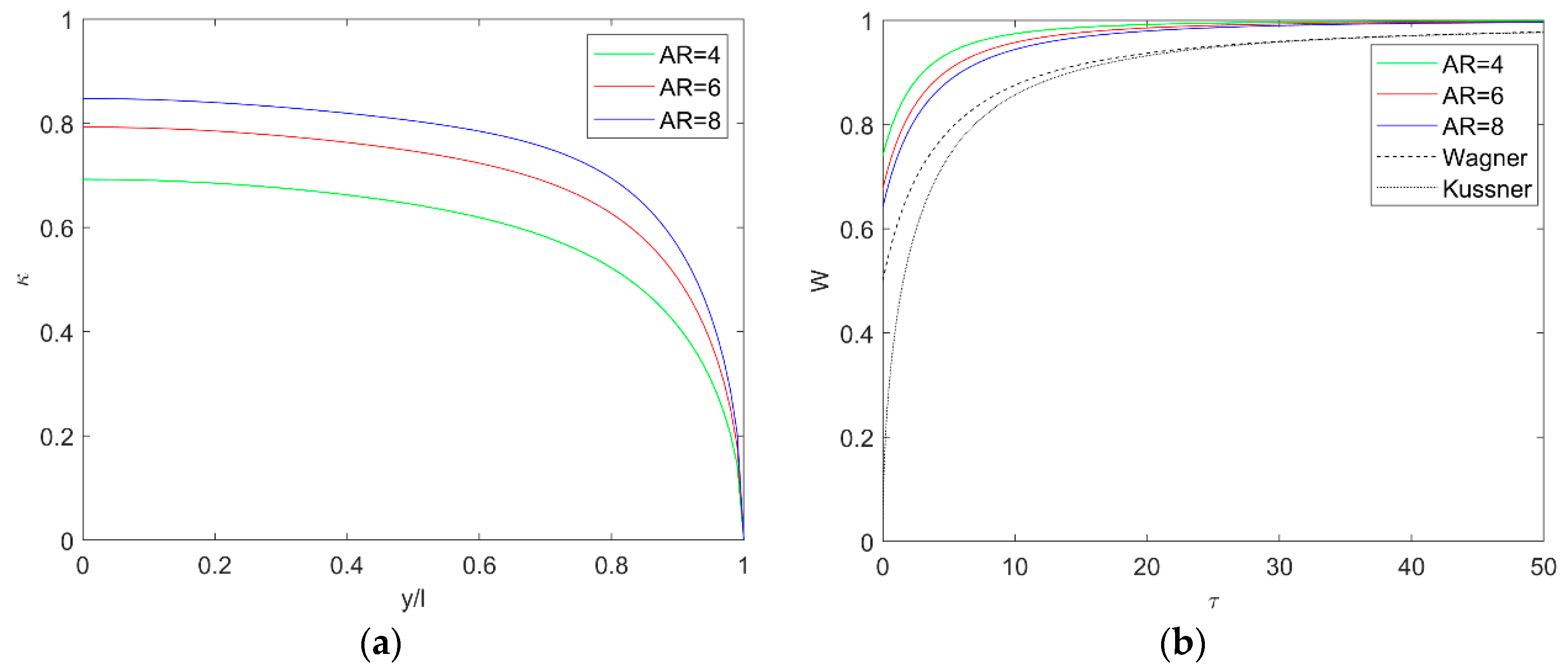
The first three (odd) sinusoidal terms granted convergence of the (symmetric) normalised lift distribution shown in Figure A1, where the lift-deficiency function due to a unit step in angle of attack is also shown. These analytical results show good agreement with the numerical ones and provide sound comparisons.
Figure A1.
Lift-scaling (a) and lift-deficiency (b) functions for flat rectangular wings of different aspect ratios.
Figure A1.
Lift-scaling (a) and lift-deficiency (b) functions for flat rectangular wings of different aspect ratios.

Appendix A.1. Steady Lift Distribution
Prandtl’s equations for the sectional flow circulation and downwash angle are generalised as [57,58]:
respectively, where is a dummy integration variable running along the wing span, whereas AR represents the ratio between the latter and mean chord for trapezoidal and elliptical planforms. This refined lifting-line model then gives a correct estimate of the downwash towards the wing root but underestimates the lift decay towards the wing tips, where VLM and DLM prescribe a stronger vortex effect. Inthis respect, note that tapering the wing increases the aspect ratio while decreasing the wing downwash and hence reduces the challenges to the MST [27].
Due to Glauert’s integral (in principal value) [76] and being , adopting Prandtl’s expansion for the circulation gives [56]:
and results in a modified system of linear algebraic equations for the lifting-line model [57,58]:
where Prandtl’s original equations [56] are asymptotically resumed for slender wings. Odd and even Fourier terms still give symmetric and antisymmetric circulation distributions, respectively; the coefficients are then found by solving such linear system in a least-squares sense [133], on wing sections at various spanwise stations , with running from tip to tip along the span. Note that for , while the singularities at can be lifted by multiplying both sides of the equation by . Thus, the scaling function coefficients are derived from:
Oswald’s efficiency factor [83] is finally used to write the lift coefficient derivative for the entire wing; the unified LLT [86] shall be employed for slender wings with significant sweep angle. Within a proper orthogonal decomposition (POD) perspective [26], scaling function and aerofoil differential pressure coefficient distribution may be interpreted as the dominant (normalised) modes of the load in the spanwise and chordwise directions, respectively, with the angle of attack driving their amplitude.
Appendix A.2. Unsteady Lift Development
For finite wings, the influence of the tip vortices on the unsteady lift distribution along the wing span may be calculated based on lifting line model as a function of the wing aspect ratio [29] (which introduces the dependency of the air load on the finite spanwise dimension) and the aerodynamic derivatives of the wing may be obtained from the ones of its airfoil section [39].
As an effective, simplified approach, a single vortex-ring is considered for modeling the total (lumped) wing circulation [59]. The bound vortex is placed at the AC line, as per thin airfoil theory, while the wing-tip vortices are trailed parallel to the free-stream; a single CP for the total downwash is then consistently placed at the wing’s root, where the flow’s non-penetration boundary condition is satisfied. All vortex lines have the same (lumped) intensity and the shed vorticity travels towards infinity with half the reference speed from half the wing’s root chord behind the control point, hence stretching the vortex-ring and increasing the wake length; when the wake eventually approaches infinity, its influence fades away and the steady condition is asymptotically obtained. The influence of both tip vortices and unsteady wake on the wing lift is therefore calculated using the simplest implementation of unsteady lifting line theory [84,85,86] and the load build-up is obtained as a function of the aspect ratio.
Considering all contributions due to bound, trailed and shed vortices of the vortex-ring, the wing lift-deficiency coefficient from a unit step in the angle of attack is calculated based on Kutta-Joukowsky theorem and Biot-Savart law as [59]:
with the initial (step-like) and asymptotic (steady) behaviours respectively given by:
Garrick’s approximation [106] of Wagner’s function for thin aerofoil is correctly resumed in the limit of infinitely slender wing [30]. Nevertheless, due to the inherent limitations of the vortex-system employed, the initial and final values of the lift coefficient are not very accurate and shall rather be provided by other higher-fidelity sources, with a suitable general expression being [39,83]:
where is the elliptic integral giving the ratio of the semi-perimeter to the span for an elliptical planform with the same aspect ratio, whereas only when Prandtl’s original equations [56] are considered. Using linear mapping [77], the lift-deficiency coefficient from a unit step in the angle of attack may finally be approximated as:
where both asymptotic and initial conditions are automatically satisfied. It is worth stressing that this unsteady aerodynamic model was originally derived for slender wings with significant sweep angle and taper ratio [59].
Finally, in order to estimate the lift-deficiency function from a unit sharp-edge gust within the standard “frozen” approach [134], that from a unit step in the angle of attack shall be multiplied by the ratio between Kussner’s [31] and Wagner’s functions (introducing the two-dimensional effect of the gust penetration); all wing sections encountering the gust at the same time, Kussner’s function for thin airfoils is then automatically resumed in the limit of infinite wings. Note that this is roughly equivalent to convolving the lift-deficiency coefficient from a unit step in the angle of attack with a fictitious angle of attack derived from the Laplace transform of the ratio between Sears’ [34,35] and Theodorsen’s functions (representing a delay function for the two-dimensional flow). Of course, the wind gust penetration delays the circulation growth and hence reaches the asymptotic (steady) lift. In the general case of swept wings [59], the gust-entry delay relative to each section is geometrically known and shall also be considered in order to obtain the lift build-up due to a unit a sharp-edge gust normal to the reference airflow, which is purely circulatory and acts at the AC.
References
- Cavagna, L.; Ricci, S.; Travaglini, L. NeoCASS: An Integrated Tool for Structural Sizing, Aeroelastic Analysis and MDO at Conceptual Design Level. Prog. Aerosp. Sci. 2011, 47, 621–635. [Google Scholar] [CrossRef]
- Alexandrov, N.M.; Hussaini, M.Y. Multidisciplinary Design Optimization: State of the Art; Proceedings in Applied Mathematics Series, 80; SIAM: Philadelphia, PA, USA, 1997. [Google Scholar]
- Martins, J.R.R.A.; Lambe, A.B. Multidisciplinary Design Optimization: A Survey of Architectures. AIAA J. 2013, 51, 2049–2075. [Google Scholar] [CrossRef] [Green Version]
- Vanderplaats, G.N. Numerical Optimization Techniques for Engineering Design: With Applications; Series in Mechanical Engineering; McGraw Hill: New York, NY, USA, 1984. [Google Scholar]
- Pike, E.C. Manual on Aeroelasticity; AGARD-R-578-71; AGARD: Neuilly sur Seine, France, 1971. [Google Scholar]
- Livne, E. The Future of Aircraft Aeroelasticity. J. Aircr. 2003, 40, 1066–1092. [Google Scholar] [CrossRef]
- Kesseler, E.; Guenov, M. Advances in Collaborative Civil Aeronautical Multidisciplinary Design Optimization; Progress in Astronautics and Aeronautics Series, 233; AIAA: Reston, VA, USA, 2010. [Google Scholar]
- Bungartz, H.J.; Schafer, M. Fluid-Structure Interaction: Modelling, Simulation, Optimization; Lecture Notes in Computational Science and Engineering, 53; Springer: Berlin, Germany, 2006. [Google Scholar]
- Dhatt, G.; Lefrancois, E.; Touzot, G. Finite Element Method; Numerical Methods Series; Wiley: Hoboken, NJ, USA, 2013. [Google Scholar]
- Chung, T.J. Computational Fluid Dynamics; Cambridge Press: Cambridge, UK, 2002. [Google Scholar]
- Cavagna, L.; Quaranta, G.; Ghiringhelli, G.L.; Mantegazza, P. Efficient Application of CFD Aeroelastic Methods Using Commercial Software. In Proceedings of the 11th IFASD, Munich, Germany, 28 June–1 July 2005. [Google Scholar]
- Romanelli, G.; Serioli, E.; Mantegazza, P. A “Free” Approach to Computational Aeroelasticity; AIAA-2010-176; AIAA: Reston, VA, USA, 2010. [Google Scholar]
- Sucipto, T.; Berci, M.; Krier, J. Gust Response of a Flexible Typical Section via High- and (Tuned) Low-Fidelity Simulations. Comput. Struct. 2013, 122, 202–216. [Google Scholar] [CrossRef]
- Berci, M.; Mascetti, S.; Incognito, A.; Gaskell, P.H.; Toropov, V.V. Dynamic Response of Typical Section Using Variable-Fidelity Fluid Dynamics and Gust-Modeling Approaches—With Correction Methods. J. Aerosp. Eng. 2014, 27, 04014026. [Google Scholar] [CrossRef]
- Farhat, C.; Lesoinne, M.; Le Tallec, P. Load and Motion Transfer Algorithms for Fluid/Structure Interaction Problems with Non-Matching Discrete Interfaces: Momentum and Energy Conservation, Optimal Discretization and Application to Aeroelasticity. Comput. Methods Appl. Mech. Eng. 1998, 157, 95–114. [Google Scholar] [CrossRef]
- Cizmas, P.G.A.; Gargoloff, J.I. Mesh Generation and Deformation Algorithm for Aeroelasticity Simulations. J. Aircr. 2008, 45, 1062–1066. [Google Scholar] [CrossRef]
- Heil, M.; Hazel, A.L.; Boyle, J. Solvers for Large-Displacement Fluid–Structure Interaction Problems: Segregated Versus Monolithic Approaches. Comput. Mech. 2008, 43, 91–101. [Google Scholar] [CrossRef]
- Sheldon, J.P.; Miller, S.T.; Pitt, J.S. Methodology for Comparing Coupling Algorithms for Fluid-Structure Interaction Problems. World J. Mech. 2014, 4, 54. [Google Scholar] [CrossRef]
- Kloppel, T.; Popp, A.; Wall, W.A. Interface Treatment in Computational Fluid-Structure Interaction. In Proceedings of the 3rd ECCOMAS COMPDYN, Island of Corfu, Greece, 26–28 May 2011. [Google Scholar]
- Farhat, C.; Lakshminarayan, V. An ALE Formulation of Embedded Boundary Methods for Tracking Boundary Layers in Turbulent Fluid-Structure Interaction Problems. J. Comput. Phys. 2014, 263, 53–70. [Google Scholar] [CrossRef]
- Berci, M.; Toropov, V.V.; Hewson, R.W.; Gaskell, P.H. Multidisciplinary Multifidelity Optimisation of a Flexible Wing Aerofoil with Reference to a Small UAV. Struct. Multidiscip. Optim. 2014, 50, 683–699. [Google Scholar] [CrossRef]
- Quarteroni, A.; Rozza, G. Reduced Order Methods for Modeling and Computational Reduction; MS&A, 9; Springer International Publishing: Cham, Switzerland, 2014. [Google Scholar]
- Qu, Z.Q. Model Order Reduction Techniques with Applications in Finite Element Analysis; Springer: London, UK, 2004. [Google Scholar]
- Ghoreyshi, M.; Jirasek, A.; Cummings, R.M. Reduced Order Unsteady Aerodynamic Modeling for Stability and Control Analysis Using Computational Fluid Dynamics. Prog. Aerosp. Sci. 2014, 71, 167–217. [Google Scholar] [CrossRef]
- Gennaretti, M.; Mastroddi, F. Study of Reduced-Order Models for Gust-Response Analysis of Flexible Fixed Wings. J. Aircr. 2004, 41, 304–313. [Google Scholar] [CrossRef]
- Ripepi, M.; Verveld, M.J.; Karcher, N.W.; Franz, T.; Abu-Zurayk, M.; Görtz, S.; Kier, T.M. Reduced Order Models for Aerodynamic Applications, Loads and MDO; DLRK-2016-420057; DLR: Braunschweig, Germany, 2016. [Google Scholar]
- Berci, M. Semi-Analytical Static Aeroelastic Analysis and Response of Flexible Subsonic Wings. Appl. Math. Comput. 2015, 267, 148–169. [Google Scholar] [CrossRef]
- Sitaraman, J.; Baeder, J.D. Computational-Fluid-Dynamics-Based Enhanced Indicial Aerodynamic Models. J. Aircr. 2004, 41, 798–810. [Google Scholar] [CrossRef]
- Anderson, J.D. Fundamentals of Aerodynamics; Series in Aeronautical and Aerospace Engineering; McGraw-Hill: New York, NY, USA, 2007. [Google Scholar]
- Wagner, H. Uber die Entstenhung des Dynamischen Auftriebes von Tragflugeln. Z. Angew. Math. Mech. 1925, 5, 17–35. [Google Scholar] [CrossRef]
- Kussner, H.G. Zusammenfassender Beritch uber den Instationaren Auftrieb von Flugeln. Luftfahrtforsch 1936, 13, 410–424. [Google Scholar]
- Kayran, A. Küssner’s Function in the Sharp Edged Gust Problem—A Correction. J. Aircr. 2006, 43, 1596–1599. [Google Scholar] [CrossRef]
- Theodorsen, T. General Theory of Aerodynamic Instability and the Mechanism of Flutter; NACA 496; NACA: Washington, DC, USA, 1935. [Google Scholar]
- Von Karman, T.; Sears, W.R. Airfoil Theory for Non-Uniform Motion. J. Aeronaut. Sci. 1938, 5, 379–390. [Google Scholar] [CrossRef]
- Sears, W.R. Operational Methods in the Theory of Airfoils in Non-Uniform Motion. J. Frankl. Inst. 1940, 230, 95–111. [Google Scholar] [CrossRef]
- Katz, J.; Plotkin, A. Low Speed Aerodynamics; Cambridge Aerospace Series; Cambridge University Press: Cambridge, UK, 2001. [Google Scholar]
- Diederich, F.W. Approximate Aerodynamic Influence Coefficients for Wings of Arbitrary Plan Form in Subsonic Flow; NACA TN 2092; NACA: Washington, DC, USA, 1950. [Google Scholar]
- Diederich, F.W.; Zlotnick, M. Calculated Spanwise Lift Distributions, Influence Functions and Influence Coefficients for Unswept Wings in Subsonic Flow; NACA 1228; NACA: Washington, DC, USA, 1955. [Google Scholar]
- Jones, R.T. The Unsteady Lift of a Wing of Finite Aspect Ratio; NACA 681; NACA: Washington, DC, USA, 1940. [Google Scholar]
- Jones, W.P. Aerodynamic Forces on Wings in Simple Harmonic Motion; ARC-RM-2026; HM Stationery Office: London, UK, 1945. [Google Scholar]
- Jones, W.P. Aerodynamic Forces on Wings in Non-Uniform Motion; ARC-RM-2117; HM Stationery Office: London, UK, 1945. [Google Scholar]
- Reissner, E. Effect of Finite Span on the Airload Distributions for Oscillating Wings—Part I: Aerodynamic Theory of Oscillating Wings of Finite Span; NACA TN-1194; Massachusetts Institute of Technology: Cambridge, MA, USA, 1947. [Google Scholar]
- Reissner, E.; Stevens, J.E. Effect of Finite Span on the Airload Distributions for Oscillating Wings—Part II: Methods of Calculation and Examples of Application; NACA TN-1195; NACA: Washington, DC, USA, 1947. [Google Scholar]
- Albano, E.; Rodden, W.P. A Doublet-Lattice Method for Calculating the Lift Distribution of Oscillating Surfaces in Subsonic Flows. AIAA J. 1969, 7, 279–285. [Google Scholar] [CrossRef]
- Rodden, W.P.; Harder, R.L.; Bellinger, E.D. Aeroelastic Addition to NASTRAN; NASA CR-3094; NASA: Washington, DC, USA, 1979.
- Quick Reference Guide. In MSC Nastran; MSC Software Corporation: Newport Beach, CA, USA, 2018.
- Holmes, R.B. A Course on Optimization and Best Approximation; Lecture Notes in Mathematics, 257; Springer: Berlin, Germany, 1972. [Google Scholar]
- Leishman, J.G. Principles of Helicopter Aerodynamics; Cambridge Aerospace Series; Cambridge University Press: Cambridge, UK, 2006. [Google Scholar]
- Bisplinghoff, R.L.; Ashley, H. Principles of Aeroelasticity; Dover: Mineola, NY, USA, 2013. [Google Scholar]
- Reddy, J.N. Energy Principles and Variational Methods in Applied Mechanics; Wiley: Hoboken, NJ, USA, 2002. [Google Scholar]
- Hodges, D.H.; Pierce, G.A. Introduction to Structural Dynamics and Aeroelasticity; Cambridge Aerospace Series; Cambridge University Press: Cambridge, UK, 2002. [Google Scholar]
- Bisplinghoff, R.L.; Ashley, H.; Halfman, R.L. Aeroelasticity; Dover: Mineola, NY, USA, 1996. [Google Scholar]
- Demasi, L.; Livne, E. Structural Ritz-Based Simple-Polynomial Nonlinear Equivalent Approach—An Assessment; AIAA-2005-2093; AIAA: Reston, VA, USA, 2005. [Google Scholar]
- Fung, Y.C. An Introduction to the Theory of Aeroelasticity; Dover: Mineola, NY, USA, 1993. [Google Scholar]
- Dowell, E.H. A Modern Course in Aeroelasticity; Solid Mechanics and Its Applications, 217; Springer: Berlin, Germany, 2015. [Google Scholar]
- Prandtl, L. Applications of Modern Hydrodynamics to Aeronautics; NACA TR-116; NACA: Washington, DC, USA, 1921. [Google Scholar]
- Helmbold, H.B. Der Unverwundene Ellipsenflügel als Tragende Fläche. In Jahrbuch der Deutschen Luftfahrtforschung; Deutsche Akademie der Luftfahrtforschung: Munich, Germany, 1942; Volume I, pp. 111–113. [Google Scholar]
- Diederich, F.W. A Plan-Form Parameter for Correlating Certain Aerodynamic Characteristics of Swept Wings; NACA TN 2335; NACA: Washington, DC, USA, 1951. [Google Scholar]
- Queijo, M.J.; Wells, W.R.; Keskar, D.A. Approximate Indicial Lift Function for Tapered, Swept Wings in Incompressible Flow; NASA TP-1241; NASA: Washington, DC, USA, 1978.
- Wells, W.R. An Approximate Analysis of Wing Unsteady Aerodynamics; AFFDL-TR-79-3046; University of Dayton Research Institute: Dayton, OH, USA, 1979. [Google Scholar]
- Jones, R.T. Classical Aerodynamic Theory; NASA RP 1050; NASA: Washington, DC, USA, 1979.
- Megson, T.H.G. Aircraft Structures for Engineering Students; Elsevier Aerospace Engineering Series; Elsevier: Oxford, UK, 2007. [Google Scholar]
- Yang, B. Strain, Stress and Structural Dynamics; Elsevier: London, UK, 2005. [Google Scholar]
- Amabili, M. Nonlinear Vibrations and Stability of Shells and Plates; Cambridge University Press: Cambridge, UK, 2008. [Google Scholar]
- Berci, M.; Gaskell, P.H.; Hewson, R.W.; Toropov, V.V. A Semi-Analytical Model for the Combined Aeroelastic Behaviour and Gust Response of a Flexible Aerofoil. J. Fluids Struct. 2013, 37, 3–21. [Google Scholar] [CrossRef]
- Wright, J.R.; Cooper, J.E. Introduction to Aircraft Aeroelasticity and Loads; Aerospace Series; Wiley: Chichester, UK, 2015. [Google Scholar]
- Young, W.C.; Budynas, R.G. Roark’s Formulas for Stress and Strain; McGraw-Hill: New York, NY, USA, 2011. [Google Scholar]
- Han, S.M.; Benaroya, H.; Wei, T. Dynamics of Transversally Vibrating Beams Using Four Engineering Theories. J. Sound Vib. 1999, 225, 935–988. [Google Scholar] [CrossRef]
- Marzocca, P.; Librescu, L.; Silva, W.A. Aeroelastic Response and Flutter of Swept Aircraft Wings. AIAA J. 2002, 40, 801–812. [Google Scholar] [CrossRef]
- Craig, R.R.; Bampton, M.C.C. Coupling of Substructures for Dynamic Analyses. AIAA J. 1968, 6, 1313–1319. [Google Scholar]
- Allemang, R.J. The modal assurance criterion—Twenty years of use and abuse. Sound Vib. 2003, 37, 14–23. [Google Scholar]
- Drischler, J.A. Approximate Indicial Lift Function for Several Wings of Finite Span in Incompressible Flow as Obtained from Oscillatory Lift Coefficients; NACA TN-3639; NACA: Washington, DC, USA, 1956. [Google Scholar]
- Mateescu, D.; Seytre, J.F.; Berhe, A.M. Theoretical Solutions for Finite-Span Wings of Arbitrary Shapes Using Velocity Singularities. J. Aircr. 2003, 40, 450–460. [Google Scholar] [CrossRef] [Green Version]
- Lomax, H.; Heaslet, M.A.; Fuller, F.B.; Sluder, L. Two- and Three-Dimensional Unsteady Lift Problems in High-Speed Flight; NACA 1077; NACA: Washington, DC, USA, 1950. [Google Scholar]
- Gulcat, U. Fundamentals of Modern Unsteady Aerodynamics; Springer: Berlin, Germany, 2011. [Google Scholar]
- Glauert, H. The Elements of Aerofoil and Airscrew Theory; Cambridge Science Classics; Cambridge University Press: Cambridge, UK, 1983. [Google Scholar]
- Quarteroni, A.; Sacco, R.; Saleri, F. Numerical Mathematics; Texts in Applied Mathematics, 37; Springer: Berlin, Germany, 2007. [Google Scholar]
- Abbott, I.H.; von Doenhoff, A.E. Theory of Wing Sections: Including a Summary of Aerofoil Data; Dover: New York, NY, USA, 1959. [Google Scholar]
- Peters, D.A.; Hsieh, M.C.A.; Torrero, A. A State-Space Airloads Theory for Flexible Airfoils. J. Am. Helicopter Soc. 2007, 52, 329–342. [Google Scholar] [CrossRef]
- Pettit, G.W. Model to Evaluate the Aerodynamic Energy Requirements of Active Materials in Morphing Wings. Master’s Thesis, Virginia Polytechnic Institute and State University, Blacksburg, VA, USA, 2001. [Google Scholar]
- Kutta, M.W. Auftriebskräfte in Strömenden Flüssigkeiten. Illustrierte Aeronautische Mitteilungen 1902, 6, 133–135. [Google Scholar]
- Joukowski, N.E. Sur les Tourbillons Adjionts. Traraux de la Section Physique de la Societé Imperiale des Amis des Sciences Naturales 1906, 13, 2. [Google Scholar]
- Nita, M.F. Contributions to Aircraft Preliminary Design and Optimization. Ph.D. Thesis, Politehnica University of Bucharest, Bucharest, Romania, 2012. [Google Scholar]
- Van Holten, T. Some Notes on Unsteady Lifting-Line Theory. J. Fluid Mech. 1976, 77, 561–579. [Google Scholar] [CrossRef]
- Sclavounos, P.D. An Unsteady Lifting-Line Theory. J. Eng. Math. 1987, 21, 201–226. [Google Scholar] [CrossRef]
- Guermond, J.L.; Sellier, A. A Unified Unsteady Lifting-Line Theory. J. Fluid Mech. 1991, 229, 427–451. [Google Scholar] [CrossRef]
- Wieseman, C.D. Methodology for Matching Experimental and Computational Aerodynamic Data; NASA TM-100592; NASA: Washington, DC, USA, 1988.
- Palacios, R.; Climent, H.; Karlsson, A.; Winzell, B. Assessment of Strategies for Correcting Linear Unsteady Aerodynamics Using CFD or Test Results. In Proceedings of the 9th IFASD, Madrid, Spain, 5–7 June 2001. [Google Scholar]
- Munk, M.M. Elements of the Wing Section Theory and of the Wing Theory; NACA 191; NACA: Washington, DC, USA, 1924. [Google Scholar]
- Lippisch, A. Method for the Determination of the Spanwise Lift Distribution; NACA TM 778; NACA: Washington, DC, USA, 1935. [Google Scholar]
- Pearson, H.A. Span Load Distribution for Tapered Wings with Partial-Span Flaps; NACA 585; NACA: Washington, DC, USA, 1937. [Google Scholar]
- DeYoung, J. Theoretical Additional Span Loading Characteristics of Wings with Arbitrary Sweep, Aspect Ratio, and Taper Ratio; NACA TN 1491; NACA: Washington, DC, USA, 1947. [Google Scholar]
- DeYoung, J. Theoretical Antisymmetric Span Loading for Wings of Arbitrary Plan Form at Subsonic Speeds; NACA TN 2140; NACA: Washington, DC, USA, 1950. [Google Scholar]
- Multhopp, H. Methods for Calculating the Lift Distribution of Wings (Subsonic Lifting-Surface Theory); ARC R&M 2884; Aeronautical Research Council: London, UK, 1955. [Google Scholar]
- Simpson, R.W. An Extension of Multhopp’s Lifting Surface Theory; Cranfield CoA Report 132; Cranfield University: Bedford, UK, 1960. [Google Scholar]
- Brebner, G.G.; Lemaire, D.A. The Calculation of the Spanwise Loading Sweptback Wings with Flaps or All-Moving Tips at Subsonic Speeds; ARC R&M 3487; Aeronautical Research Council: London, UK, 1967. [Google Scholar]
- Woodward, F.A. An Improved Method for the Aerodynamic Analysis of Wing-Body-Tail Configurations in Subsonic and Supersonic Flow; NASA CR-2228; NASA: Washington, DC, USA, 1973.
- Morino, L. A General Theory of Unsteady Compressible Potential Aerodynamics; NASA CR-2464; NASA: Washington, DC, USA, 1974.
- Blair, M. A Compilation for the Mathematics Leading to the Doublet Lattice Method; WL-TR-92-3028; USAF: Washington, DC, USA, 1992.
- Fossati, M. Evaluation of Aerodynamic Loads via Reduced-Order Methodology. AIAA J. 2015, 53, 2389–2405. [Google Scholar] [CrossRef]
- Thwapiah, G.; Campanile, L.F. Nonlinear Aeroelastic Behavior of Compliant Aerofoils. Smart Mater. Struct. 2010, 19, 253–262. [Google Scholar] [CrossRef]
- Cone, C.D. The Theory of Induced Lift and Minimum Induced Drag of Non-Planar Lifting Systems; NASA TR R-139; NASA: Washington, DC, USA, 1962.
- Forrester, A.J.; Keane, A.J. Engineering Design via Surrogate Modelling: A Practical Guide; Wiley: Chichester, UK, 2008. [Google Scholar]
- Berci, M.; Gaskell, P.H.; Hewson, R.W.; Toropov, V.V. Multifidelity Metamodel Building as a Route to Aeroelastic Optimization of Flexible Wings. J. Mech. Eng. Sci. 2011, 225, 2115–2137. [Google Scholar] [CrossRef]
- Tiffany, S.H.; Adams, W.M. Nonlinear Programming Extensions to Rational Function Approximation Methods for Unsteady Aerodynamic Forces; NASA-TP-2776; NASA: Washington, DC, USA, 1988.
- Garrick, L.E. On Some Reciprocal Relations in the Theory of Nonstationary Flows; NACA-629; NACA: Washington, DC, USA, 1938. [Google Scholar]
- Heaslet, M.A.; Spreiter, J.R. Reciprocity Relations in Aerodynamics; NACA-1119; NACA: Washington, DC, USA, 1953. [Google Scholar]
- Beddoes, T.S. Practical Computation of Unsteady Lift. Vertica 1984, 8, 55–71. [Google Scholar]
- Dowell, E.H. A Simple Method for Converting Frequency Domain Aerodynamics to the Time Domain; NASA-TM-81844; NASA: Washington, DC, USA, 1980.
- Leishman, J.G.; Nguyen, K.Q. State-Space Representation of Unsteady Airfoil Behavior. AIAA J. 1990, 28, 836–844. [Google Scholar] [CrossRef]
- Tobak, M. On the Use of the Indicial-Function Concept in the Analysis of Unsteady Motions of Wings and Wing-Tail Combinations; NACA 1188; NACA: Washington, DC, USA, 1954. [Google Scholar]
- Silva, W. Discrete-Time Linear and Nonlinear Aerodynamic Impulse Responses for Efficient Use of CFD Analyses. Ph.D. Thesis, College of William & Mary, Williamsburg, VA, USA, 1997. [Google Scholar]
- Ghoreyshi, M.; Jirásek, A.; Cummings, R.M. Computational Investigation into the Use of Response Functions for Aerodynamic-Load Modeling. AIAA J. 2012, 50, 1314–1327. [Google Scholar] [CrossRef]
- Rodden, W.P. Theoretical and Computational Aeroelasticity; Crest Pub.: Columbus, OH, USA, 2011. [Google Scholar]
- Van Zyl, L.H. Aeroelastic Divergence and Aerodynamic Lag Roots. J. Aircr. 2001, 38, 586–588. [Google Scholar] [CrossRef]
- Aeroelastic Analysis User’s Guide. In MSC Nastran; MSC Software Corporation: Newport Beach, CA, USA, 2018.
- Appa, K. Finite-Surface Spline. J. Aircr. 1989, 26, 495–496. [Google Scholar] [CrossRef]
- Harder, R.L.; Desmarais, R.N. Interpolation Using Surface Splines. J. Aircr. 1972, 9, 189–191. [Google Scholar] [CrossRef]
- Lanczos, C. An Iteration Method for the Solution of the Eigenvalue Problem of Linear Differential and Integral Operators; United States Governm. Press Office: Los Angeles, CA, USA, 1950; Volume 45.
- Bellinger, D.; Pototzky, T. A Study of Aerodynamic Matrix Numerical Condition. In Proceedings of the 3rd MSC Worldwide Aerospace Conference and Technology Showcase, Toulouse, France, 24–26 September 2001. [Google Scholar]
- Giesing, J.P.; Kalman, T.P.; Rodden, W.P. Correction Factor Techniques for Improving Aerodynamic Prediction Methods; NASA CR-144967; NASA: Washington, DC, USA, 1976.
- Lawrence, A.J.; Jackson, P. Comparison of Different Methods of Assessing the Free Oscillatory Characteristics of Aeroelastic Systems; ARC CP 1084; HM Stationery Office: London, UK, 1970. [Google Scholar]
- Goland, M. The Flutter of a uniform Cantilever Wing. J. Appl. Mech. 1945, 12, A197–A208. [Google Scholar]
- Goland, M.; Luke, Y.L. The Flutter of a Uniform Wing with Tip Weights. J. Appl. Mech. 1948, 15, 13–20. [Google Scholar]
- Wang, I. Component Modal Analysis of a Folding Wing. Ph.D. Thesis, Duke University, Durham, NC, USA, 2011. [Google Scholar]
- NASA. U.S. Standard Atmosphere; NASA TM-X-74335; NASA: Washington, DC, USA, 1976.
- Banerjee, J.R. Flutter sensitivity studies of high aspect ratio aircraft wings. WIT Trans. Built Environ. 1993, 2, 374–387. [Google Scholar]
- Sotoudeh, Z.; Hodges, D.H.; Chang, C.S. Validation Studies for Aeroelastic Trim and Stability Analysis of Highly Flexible Aircraft. J. Aircr. 2010, 47, 1240–1247. [Google Scholar] [CrossRef]
- Qin, Z. Vibration and Aeroelasticity of Advanced Aircraft Wings Modeled as Thin-Walled Beams—Dynamics, Stability and Control. Ph.D. Thesis, Virginia Polytechnic Institute and State University, Blacksburg, VA, USA, 2001. [Google Scholar]
- Palacios, R.; Epureanu, B. An Intrinsic Description of the Nonlinear Aeroelasticity of Very Flexible Wings; AIAA-2011-1917; AIAA: Reston, VA, USA, 2011. [Google Scholar]
- Dunning, P.D.; Stanford, B.K.; Kim, H.A.; Jutte, C.V. Aeroelastic Tailoring of a Plate Wing with Functionally Graded Materials. J. Fluids Struct. 2014, 51, 292–312. [Google Scholar] [CrossRef] [Green Version]
- Berci, M. Semi-Analytical Reduced-Order Models for the Unsteady Aerodynamic Loads of Subsonic Wings. In Proceedings of the 5th ECCOMAS COMPDYN, Crete, Greece, 25–27 May 2015. [Google Scholar]
- Hildebrand, F.B. A Least-Squares Procedure for the Solution of the Lifting-Line Integral Equation; NACA TN 925; NACA: Washington, DC, USA, 1944. [Google Scholar]
- Hoblit, F.M. Gust Loads on Aircraft: Concepts and Applications; AIAA Education Series; AIAA: Reston, VA, USA, 1988. [Google Scholar]
Figure 1.
Real (a) and imaginary (b) parts of the first two eigenvalues for Goland’s wing flutter.

Figure 2.
FEM (a) and DLM (b) numerical arrangement, for the wings with AR = 6.

Figure 3.
First (a), second (b), third (c) and fourth (d) FEM vibration modes, for the wings with AR = 6.
Figure 3.
First (a), second (b), third (c) and fourth (d) FEM vibration modes, for the wings with AR = 6.

Figure 4.
First two bending (a) and torsion (b) exact natural vibration modes.

Figure 5.
First (a), second (b), third (c) and fourth (d) vibration frequencies for all considered wings.
Figure 5.
First (a), second (b), third (c) and fourth (d) vibration frequencies for all considered wings.
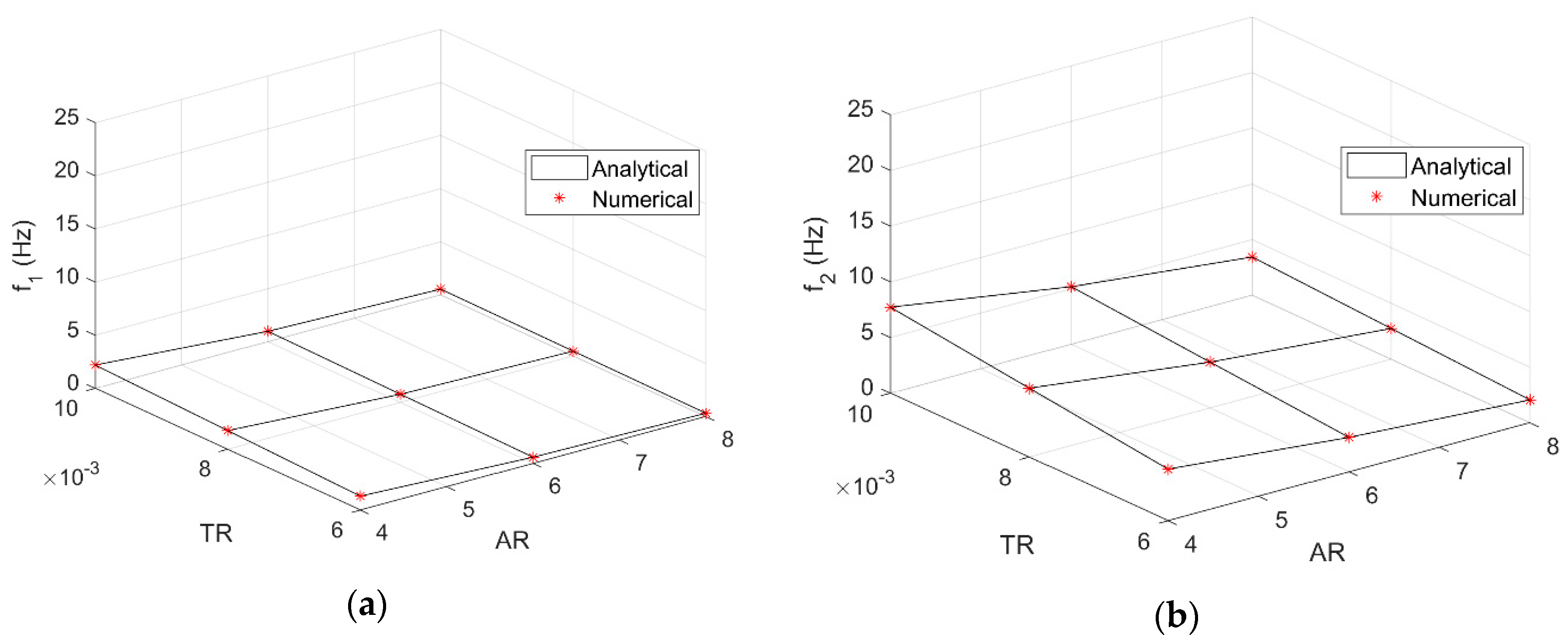
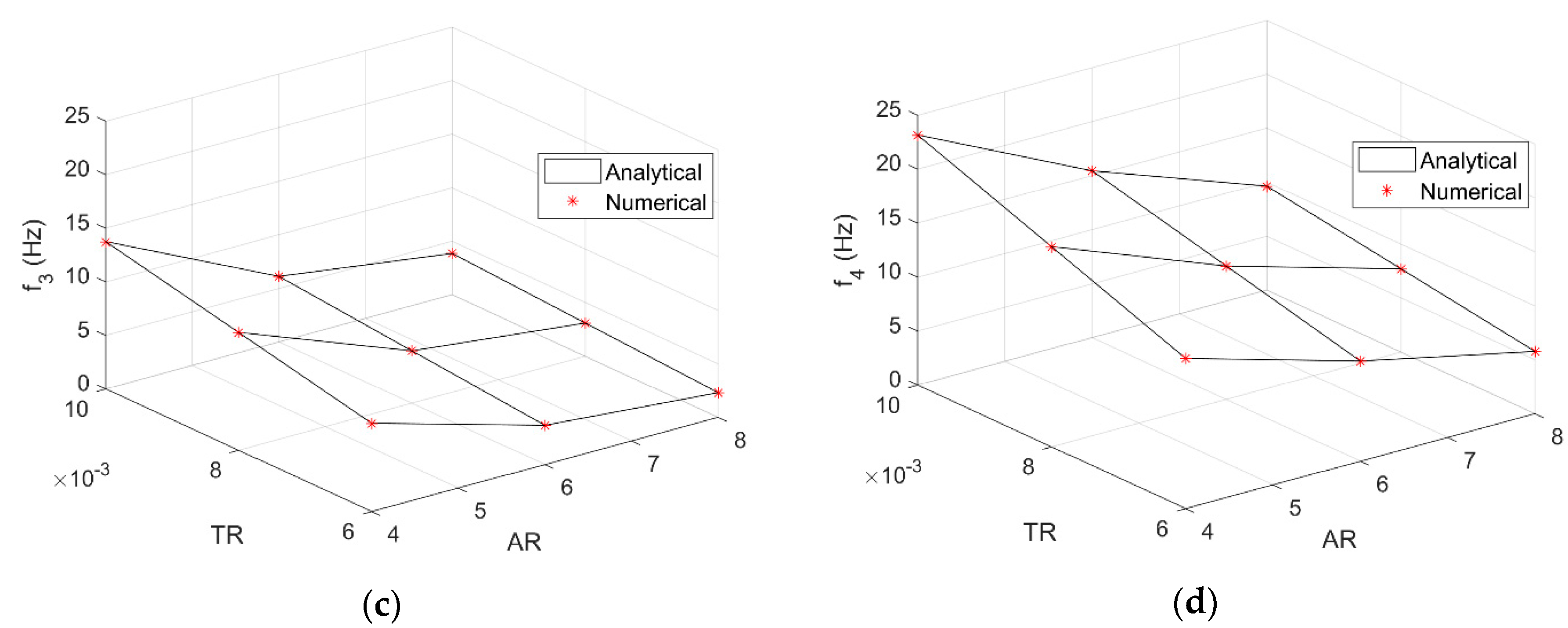
Figure 6.
Lift decay (a) and build-up (b) for flat rectangular wings with different aspect ratio: symbols = numerical solution, lines = analytical approximation.
Figure 6.
Lift decay (a) and build-up (b) for flat rectangular wings with different aspect ratio: symbols = numerical solution, lines = analytical approximation.

Figure 7.
Divergence (a) and flutter (b) speeds according to SST.
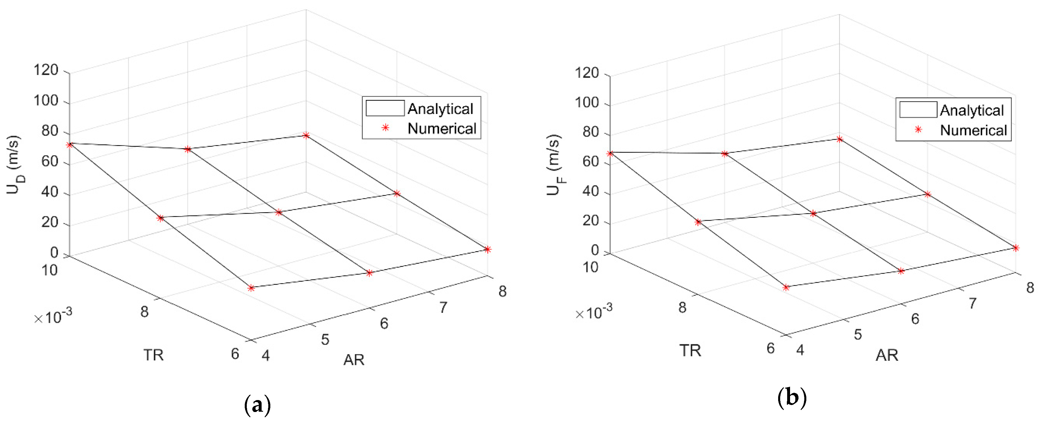
Figure 8.
Flutter frequency (a) and reduced frequency (b) speeds according to SST.
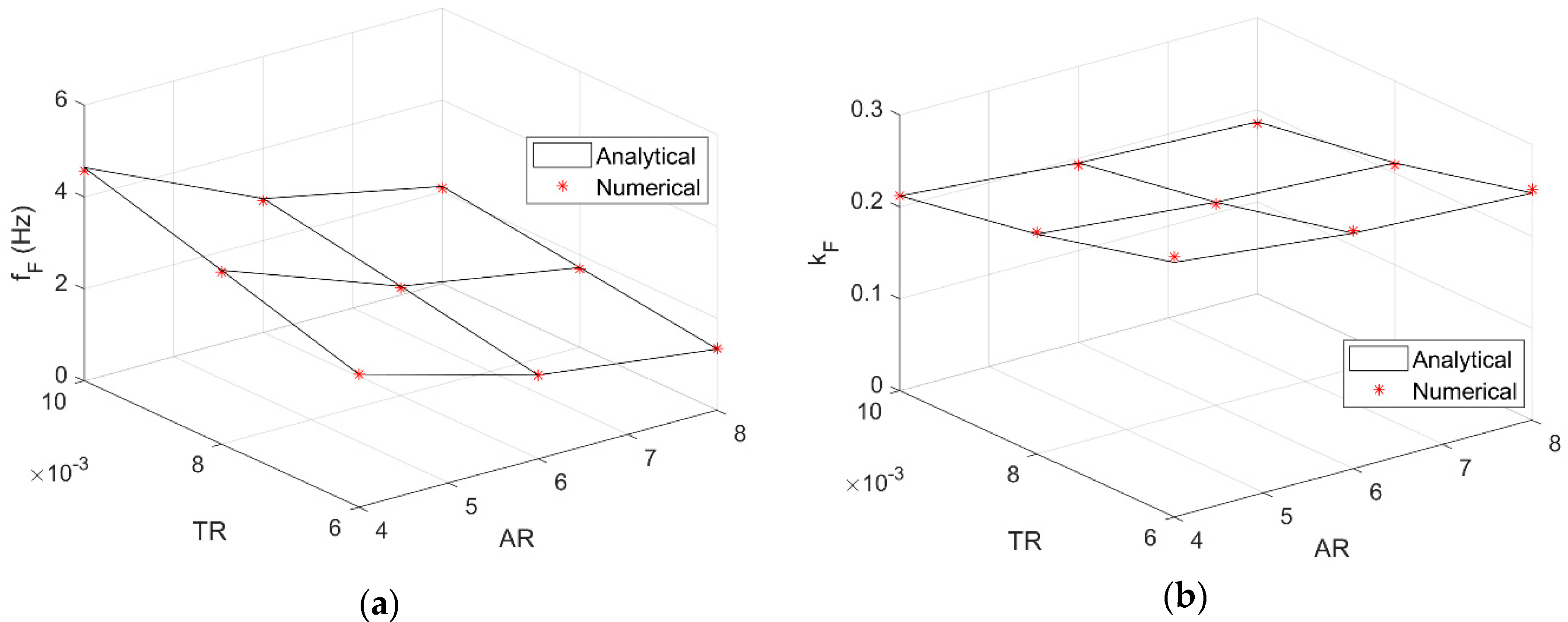
Figure 9.
Divergence (a) and flutter (b) speeds according to MST and DLM.
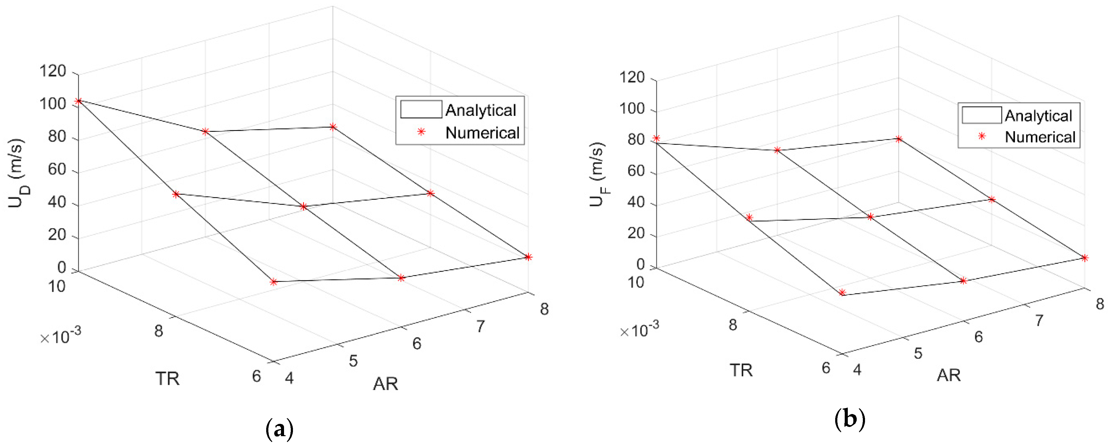
Figure 10.
Flutter frequency (a) and reduced frequency (b) speeds according to MST and DLM.


Table 1.
FEM and DLM numerical discretisation, for all considered wings.
| AR | FEM: Nodes, Elements | DLM: Spanwise, Chordwise |
|---|---|---|
| 4 | 75, 24 | 24, 12 |
| 6 | 108, 36 | 36, 12 |
| 8 | 144, 48 | 48, 12 |
Table 2.
FEM and analytical natural vibration modes, for all considered wings.
| AR | 1st Mode | 2nd Mode | 3rd Mode | 4th Mode |
|---|---|---|---|---|
| 4 | 1st Bending | 1st Torsion | 2nd Bending | 2nd Torsion |
| 6 | 1st Bending | 1st Torsion | 2nd Bending | 2nd Torsion |
| 8 | 1st Bending | 2nd Bending | 1st Torsion | 3rd Bending |
© 2018 by the authors. Licensee MDPI, Basel, Switzerland. This article is an open access article distributed under the terms and conditions of the Creative Commons Attribution (CC BY) license (http://creativecommons.org/licenses/by/4.0/).
Share and Cite
MDPI and ACS Style
Berci, M.; Cavallaro, R. A Hybrid Reduced-Order Model for the Aeroelastic Analysis of Flexible Subsonic Wings—A Parametric Assessment. Aerospace 2018, 5, 76. https://doi.org/10.3390/aerospace5030076
AMA Style
Berci M, Cavallaro R. A Hybrid Reduced-Order Model for the Aeroelastic Analysis of Flexible Subsonic Wings—A Parametric Assessment. Aerospace. 2018; 5(3):76. https://doi.org/10.3390/aerospace5030076
Chicago/Turabian StyleBerci, Marco, and Rauno Cavallaro. 2018. "A Hybrid Reduced-Order Model for the Aeroelastic Analysis of Flexible Subsonic Wings—A Parametric Assessment" Aerospace 5, no. 3: 76. https://doi.org/10.3390/aerospace5030076
Note that from the first issue of 2016, this journal uses article numbers instead of page numbers. See further details here.