Maintenance Model of Digital Avionics

Department of Electronics, National Aviation University, 03058 Kiev, Ukraine
Aerospace 2018, 5(2), 38; https://doi.org/10.3390/aerospace5020038
Submission received: 20 February 2018
/
Revised: 24 March 2018
/
Accepted: 29 March 2018
/
Published: 2 April 2018
(This article belongs to the Special Issue Challenges in Reliability Analysis of Aerospace Electronics)
Abstract
:The cost of avionics maintenance is extremely high for modern aircraft. It can be as high as 30% of the aircraft maintenance cost. A great impact on the cost of avionics maintenance is provided by a high level of No Fault Found events (NFF). Intermittent faults are the leading cause of the NFF appearance in avionics. The NFF rate for avionics systems is between 20% and 50%. The practice of avionics operation and maintenance confirms the relevance of assessing the impact of intermittent faults on the maintenance cost and the choice of such option of the maintenance management, in which the negative impact of the intermittent faults is minimized. In this paper, a new mathematical model of digital avionics maintenance is developed. Key maintenance effectiveness indicators are selected. General mathematical expressions are obtained for the average availability, mean time between unscheduled removals (MTBUR), and expected maintenance cost of single unit and redundant avionics systems, which are subject to permanent failures and intermittent faults. The dependence of the maintenance effectiveness indicators on the rate of permanent failures and intermittent faults is investigated for the case of exponential distribution of time to failures and faults. The dependence of average availability on the number of spare units in the airline’s warehouse is also analyzed. On the base of the proposed maintenance model, different options of avionics maintenance management are considered. Numerical examples illustrate how to reduce the expected maintenance cost of avionics systems.

1. Introduction
Modern aircraft use two types of avionics architecture: federated avionics (FA) and integrated modular avionics (IMA) [1,2]. In FA architecture, each system has a dedicated processing unit, and the hardware of the processing unit is not used by any other system. Each processing unit is loosely associated with the processing units of other functions. FA architecture assumes the use of a separate line replaceable unit (LRU) for each avionics function and interconnection of each LRU with others via point-to-point data buses such as ARINC 429. One of the drawbacks of FA architecture is that it is difficult to expand. Any additional LRUs require additional cable communication with existing LRUs. FA architecture requires long cable runs to connect far located LRUs that increase weight and can lead to reliability problems [3]. Until the late 1990s, the digital avionics of most civil aircraft, including the Boeing and Airbus families, was based on the FA architecture principle. The basis of the IMA is an open network architecture and a single computing platform. At the same time, system functions are performed by software applications that share common computing resources. In the IMA, the computing system represents a set of LRMs such as processor modules, memory modules, network switch modules, power modules etc. The design of LRM is based on a single standard, ensuring the principle of unification and interchangeability. Compared to the FA architecture, the transition to the IMA architecture significantly reduces the weight and cost of aircraft equipment. In the IMA architecture, much of the functionality of a traditional LRU is performed by a special application. Standalone applications are located in the common IMA modules called core processing input/output (I/O) modules (CPIOMs). Each CPIOM integrates hardware and software functions and places them in the same computing and storage resources as well as providing I/O interface to some conventional avionics LRUs. In order to connect the traditional avionics LRUs, additional LRMs, called I/O modules, are also included in the IMA architecture. The dialogue between the LRMs is conducted via avionics data communication networks (ADCN) over the avionics full-duplex switched Ethernet (AFDX) compliant with the ARINC 664 standard. The IMA architecture connects all LRMs to the ADCN network, with all information routed to the appropriate LRM through the AFDX switch. The Boeing 777 was the first commercial aircraft with partially introduced IMA architecture. The Boeing 777 uses the IMA concept to implement only some of the important functions previously performed by independent LRUs (flight control, communications control, aircraft condition monitoring). In the A380, the IMA concept was implemented for the most functions [4]. The A380 avionics comprises 30 LRMs and 22 programming functions, which are located in the CPIOMs [5]. The ADCN communications network comprises 16 AFDX switches and corresponding cables. The switches perform connection of 8 IOMs, 22 CPIOMs, and 50 LRUs with AFDX interface [4,5]. To reduce the number of connections from the cockpit control panel to avionics cabin computers, the controller area network (CAN) bus is used for the A380 avionics [6]. Although Airbus began to make extensive use of the CAN bus to reduce cabling on the A380, the popular ARINC 429 bus is still used to connect the radio control panels in the cockpit to the avionics LRUs.
Thus, modern avionics includes a large number of the LRMs and LRUs. In turn, each LRU/LRM consists of several printed circuit board assemblies, which are called shop replaceable units (SRUs). Modern LRUs and LRMs usually have built-in test equipment (BITE) for continuous monitoring during flight. In accordance with the design of modern avionics, the following three maintenance levels are typically considered: organization maintenance level (O-level), intermediate maintenance level (I-level), and depot maintenance level (D-level). The O-level is a flight-line maintenance where the LRU/LRM can be removed and replaced for a short period of time. The spare parts at the O-level are the LRUs/LRMs. Intermediate maintenance is conducted at a dedicated workshop to repair the removed LRUs/LRMs by replacing the failed SRUs. The spare parts at this maintenance level are the SRUs. Automated test equipment (ATE) is commonly used at the I-level maintenance. The failed SRUs are repaired at the D-level maintenance, where the spare parts are non-repairable electronic components.
Modern avionics systems are redundant systems. Therefore, each LRU/LRM operates up to a safe failure that is registered by the BITE during flight. The failed LRUs/LRMs are replaced by spare LRUs/LRMs at the O-level maintenance. This maintenance strategy is called a breakdown maintenance strategy. In [7] it is stated that “intermittent faults are regarded as the most difficult class of faults to diagnose and are cited as one of the main root causes of No Fault Found.” Intermittent faults are mechanical by nature. They occur due to faults of electrical wiring, solder joints, screening braid, connectors, metal lines of integrated circuits, etc. Modern electronic components are reliable, so the intermittent discontinuity between printed circuit board components is becoming the main cost driver [8]. Conventional ATE cannot detect intermittent faults that cause NFF for the following reasons [8,9]:
- (1)
- Monitored object parameters are usually tested only once for a short period of time, which usually does not coincide with the intermittent fault event time;
- (2)
- Digital averaging, scanning, and sampling of the test signal miss out intermittent faults;
- (3)
- The removed LRUs/LRMs are tested in the laboratory rather than in the operating environment where faults occur; the electrical wiring interconnect system is also tested in a static environment;
- (4)
- Conventional ATE are designed to detect permanent failures, faulty components, as well as short circuits and breaks in electrical circuits, and are not capable of intermittent fault diagnostics;
- (5)
- Intermittent faults that cause NFF do not correspond to any certain failure pattern.
The breakdown maintenance strategy may be inefficient at a high incidence of the NFF events because traditional ATE cannot detect intermittent faults and the same intermittent fault may occur again on the next flight. As indicated in [10], the estimated level of NFF for avionics is from 20% to 50%, and, moreover, avionics components account for 80.4% of all unconfirmed failures, which, in addition, leads to 26.6% of unscheduled removals of avionics LRUs/LRMs [11]. The main reason for unconfirmed failures of electronic LRUs/LRMs is the occurrence of intermittent faults in flight [12]. The negative impact of unconfirmed failures on airline operations includes increased service time, disruption of flight regularity, and an increase in spare LRUs and LRMs, which ultimately leads to an increase in the life cycle cost of avionics systems. Thus, the operational practices in commercial aviation confirm the relevance of assessing the impact of intermittent faults on the life cycle costs of avionics systems as well as the option of selecting a maintenance organization that minimizes the negative impact of intermittent faults.
The growing interest in assessing the cost of avionics maintenance is manifested in a large number of publications on this topic. A stochastic model evaluating the lifecycle cost associated with the application of prognostic health management (PHM) to helicopter avionics was considered in [13]. However, the impact of intermittent faults on the lifecycle cost of helicopter avionics was not assessed in this model. Mathematical model of a periodically monitored avionic LRU was considered in [14]. Equations of availability and expected maintenance costs of redundant avionics systems were derived. However, this model cannot be applied to modern avionics systems, which are continuously monitored. And, moreover, the proposed model does not consider the impact of intermittent faults on the maintenance effectiveness indicators. Avionics hardware lifecycle cost model was proposed in [15]. The model considered such drivers of the life-cycle costs as type of technology, percentage of new designs, weight, volume, design reliability, and operational reliability in respect to permanent failures. Intermittent faults were not included into the model. Different maintenance strategies related to the presence of NFF were considered in [16]. Statistics on NFF is analyzed, according to which the percentage of NFF in military avionics is about 70%. The proposed cost equations are empirical and can only be used for a given percentage distribution of the confirmed and unconfirmed failures. The structural-logical model of the main cost drivers of the total cost of NFF consequences was considered in [17]. The conducted analysis shows how the most suitable drivers can be selected to represent aggregate costs due to NFF. This article shows the relevance of the task of quantifying the cost of the NFF effects, but it does not contain mathematical or other models to solve this problem. A maintenance model of a continuously tested single-unit digital system subject to revealed and unrevealed failures, and intermittent faults was considered in [18]. The derived availability expression is valid only for the systems with continuous operation. Avionics systems are operated with alternation of flights and landings. Therefore, the proposed mathematical model cannot be used to estimate the availability of avionics systems. An empirical model to estimate the unit cost per hour depending on the total flight time, aircraft size, load factor, average flight time, exchange rate, number of passengers per airline, and gross domestic production was proposed in [19]. The proposed cost equation is purely economic in nature and cannot be used to select the optimal option of avionics maintenance.
The following references do not relate to mathematical models of avionics maintenance, which are the subject of this study. However, these references are important to understand the proposed mathematical model for assessing the operational reliability of avionics LRUs/LRMs. The strategy of detection of intermittent faults is analyzed, in which testing is carried out at regular intervals in [20]. An exponential time distribution to a permanent failure and intermittent fault is assumed. The optimal testing frequency is determined, which maximizes the probability of detecting an intermittent fault upon its first appearance. This model is not suitable for assessing the operational reliability because avionics systems are monitored continuously in flight, rather than periodically. A Markov model of general-purpose reliability with three states for fault-tolerant systems with both permanent failures and intermittent faults was considered in [21]. A comparison is made between the reliability of the duplex and redundant systems in the presence of permanent failures and intermittent faults. The proposed model can only be used for the systems with continuous operation. A reliability model for determining the optimal frequency of testing intermittent faults in the built-in pipelined processor by the criterion of the minimum cost of testing was considered in [22]. The Markov model with continuous time and two states is used for probabilistic modeling of intermittent faults. This model can be used only for the systems with periodic testing of the state, operating in continuous mode. A model for studying the reliability of digital systems subject to both permanent failures and intermittent faults was considered in [23]. The reliability evaluation of a digital system is based on the Markov model containing three states. This model assumes continuous operation of the digital system, and therefore cannot be used to assess the operational reliability of avionics systems. The strategy of imperfect checks to detect intermittent faults in a computer system was investigated in [24]. The system is checked at periodic times and its fault with a certain probability is detected in the next time of checking. The expected cost to intermittent fault detection is determined. This model can be used only for systems with periodic testing and continuous operation. The impact of various scenarios for restoring the processor after the occurrence of intermittent faults on its performance was assessed in [25]. To achieve this goal, the operation of a fault-tolerant multi-core processor is simulated in the presence of intermittent faults, subject to exponential and Weibull distribution. The simulation shows that 40% of the processor faults are intermittent by nature, and 60% are permanent. The results of this study can be used to select the distribution law of time to intermittent fault in digital LRUs/LRMs of avionics systems. Mathematical maintenance models of avionics LRUs subject to permanent failures and intermittent faults were considered in [26,27]. However, in order to determine the operational reliability indicators in these models, it is necessary to know the conditional probabilities of occurrence and non-occurrence of intermittent faults during flight. These probabilities are not easy to derive for an arbitrary probability distribution function (PDF) of time to intermittent fault.
The aim of this article is to develop a convenient for practical calculations mathematical model of digital avionics’ operation and maintenance, which allows us to choose the optimal option of maintenance organization. In this article, mathematical models have been developed to evaluate the operational reliability of continuously monitored LRUs/LRMs and redundant avionics systems over a finite time interval, which, unlike known models, take into account the influence of both permanent failures and intermittent faults.
2. Maintenance Model
This section outlines the step by step development of the avionics LRU/LRM maintenance model.
2.1. Possible States of LRU/LRM
The mathematical model of the LRM/LRU operation and maintenance is developed over a finite time interval (0, T). During flight the LRM/LRU is continuously monitored by BITE, and in the event of a permanent failure, the LRM/LRU is turned off. In the event of an intermittent fault, the LRM/LRU will not normally switch off during flight. However, the information about this event is usually recorded by the on-board computer. If the LRM/LRU fails permanently or intermittently during flight, after aircraft landing at the home airport it will be dismantled and directed to repair. Further, we assume that after repair the LRM/LRU becomes as good as new. At any time t in the interval (0, T), the LRU/LRM may be in one of the following states: Δ1, if at time t the LRM/LRU is operable; Δ2, if at time t the LRM/LRU is inoperable due to the detected permanent failure; Δ3, if at time t the LRM/LRU is in O-level maintenance; Δ4, if at time t the LRM/LRU is in the state of waiting for a spare LRM/LRU from the airline warehouse; Δ5, if at time t the LRM/LRU is shipped to repair or from repair; Δ6, if at time t the LRM/LRU is repaired due to an intermittent fault; Δ7, if at time t the LRM/LRU is repaired due to a permanent failure.
2.2. Mean Times of Staying the LRU/LRM in Different States
According to [28,29], the average system availability is the ratio of the uptime to the sum of the up and downtime. To find the average availability of the LRU/LRM, it is necessary to determine the average time of staying the LRU/LRM in the states during one regenerative cycle in the interval (0, T). We denote by the time spent by the LRM/LRU in the state (). First, we determine the mean time of finding the LRU/LRM in the state in the interval (0, Т). Let X and Z be, respectively, the random time to a permanent failure and intermittent fault with the PDF ω(x) and f(z), and cumulative distribution function (CDF) Ω(x) and F(z). Assume that the LRU/LRM works being operable till time υ, where and is the flight duration. Then, the LRU/LRM will be in the state for the time , if an intermittent fault occurs during -th flight, where . Further, the LRU/LRM will work for the time , if from time point till time point there is no intermittent fault. Similarly, the arguments are constructed for .
Using the formula of mathematical expectation for a discrete random variable, we determine the conditional mathematical expectation of the time spent by the LRU/LRM in the state under the condition that a permanent failure occurs at the time .
Applying to (1) the formula of complete mathematical expectation, we determine the mean time of staying the LRU/LRM in the state
Let us determine . If an intermittent fault does not occur till moment and a permanent failure occurs at the time , where , then the conditional mathematical expectation of the time spent by the LRU/LRM in the state is equal to
Applying to (3) the formula of complete mathematical expectation, we determine the time of staying the LRU/LRM in the state
If the duration of the maintenance operations are constant over the interval (0, T), the mean times spent by the LRU/LRM in the states are determined by the following formulas:
where is the average duration of maintenance operations at the O-level, is the average time of waiting the spare LRM/LRU from the warehouse, is the average scheduled stop time of the aircraft at the airport, and is the average time of shipping the failed LRM/LRU to the repair and back.
If an intermittent fault occurs during -th flight and until this moment there is no permanent failure, the conditional mathematical expectation of the time spent by the LRU/LRM in the state is equal to
where is the average time of the LRU/LRM repair due to an intermittent fault.
Applying to (12) the formula of complete mathematical expectation, we get
If a permanent failure occurs during -th flight and until moment there is no intermittent fault, the conditional mathematical expectation of the time spent by the LRU/LRM in the state is equal to
where is the average time of the LRU/LRM repair due to a permanent failure.
Applying to (10) the formula of complete mathematical expectation gives
Electronic avionics LRUs/LRMs have complex design and include a large number of components. Extrinsic and intrinsic failure mechanisms of these components may lead the units to failure. These failure mechanisms can combine together forming a constant failure rate, which is only possible with an exponential distribution of time to failure [30]. Therefore, as indicated in [31], the exponential distribution of time to permanent failure can be used for many avionics LRUs. Let and represent the PDF of time to permanent failure and intermittent fault, respectively, where and are, respectively, the rate of permanent failures and intermittent faults. Substituting and into (2), (4), (9), and (11), we obtain
2.3. Availability and Unavailability of Avionics Systems
The average availability of the avionics LRU/LRM can be determined by the following formula:
Figure 1a,b show a 3D dependence of the average availability on the rate of intermittent faults and permanent failures under exponential distribution when T = 5000 h, τ = 4 h, , , and . The difference between plots is that and for Figure 1a, and and for Figure 1b. As can be seen in Figure 1a,b, availability decreases with increasing the rate of both permanent failures and intermittent faults. However, the rate of the permanent failures has slightly greater impact on the average availability than the rate of the intermittent faults. From Figure 1a follows that the average availability begins to decrease significantly when . For , the average availability does not depend on the rate of intermittent faults. The dependence of the average availability on the rate of permanent failures and intermittent faults in Figure 1b is similar. However, the average availability begins to decrease significantly when and does not depend on the rate of intermittent faults for . Thus, intermittent faults have a significant negative impact on the availability of avionics LRUs/LRMs and this impact becomes stronger when the repair time is longer.
Modern avionics systems are redundant systems. Usually, active redundancy is used [32]. Using the method of structural functions [33], it is easy to prove that, for a parallel structure of avionics system with n identical LRUs/LRMs, the average unavailability is calculated by the following formula:
Equation (17) does not include the mean times of staying the LRU/LRM in the states , since it is not used in these states on the aircraft board.
For the m-out-of-n structure of the avionics system, the average unavailability is given by
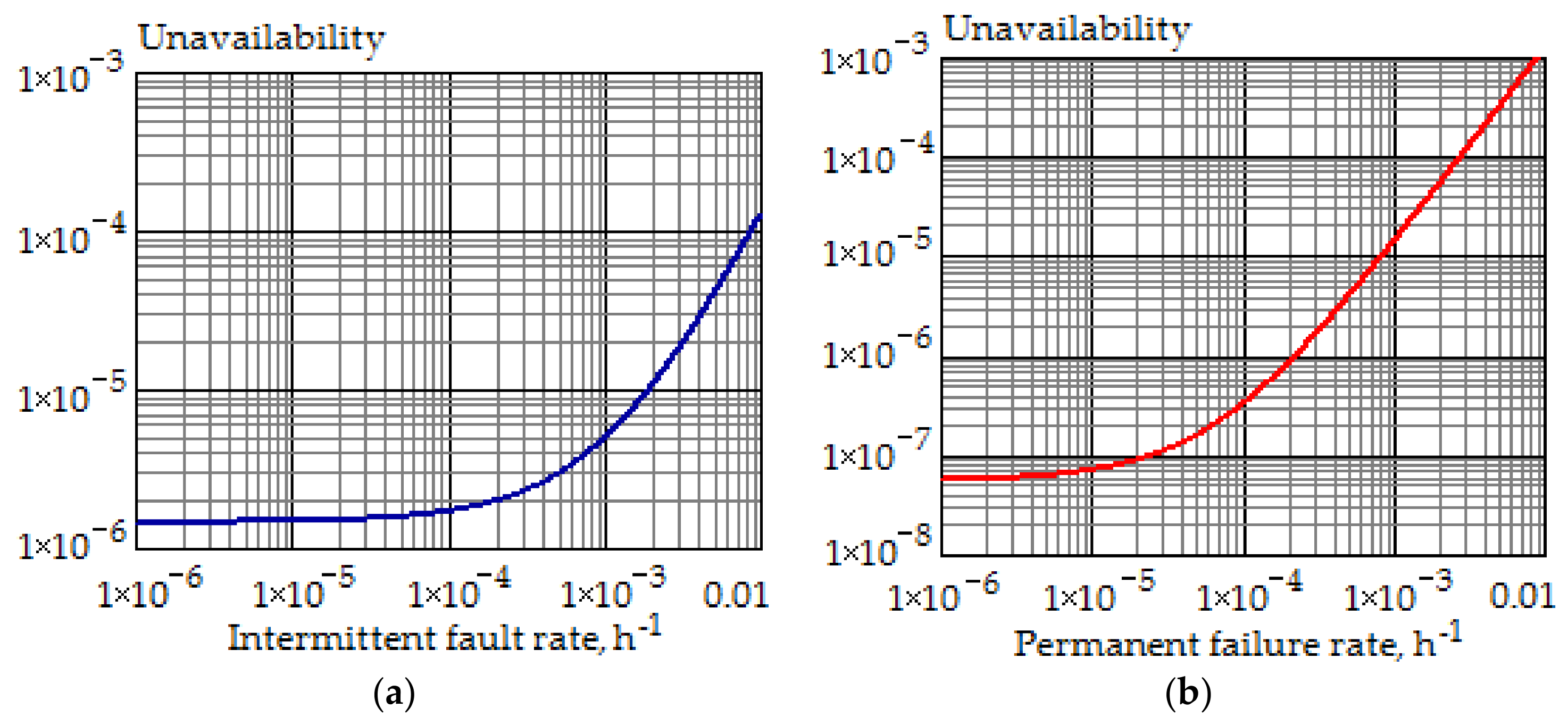
Figure 2a,b show the dependence of unavailability of the duplicated avionics system on the rate of intermittent faults (a) and permanent failures (b) for , , and . As can be seen from the comparison of Figure 2a,b, the rate of permanent failures has a greater impact on the unavailability than the rate of the intermittent faults. It should be also noted that the unavailability begins to increase significantly when .
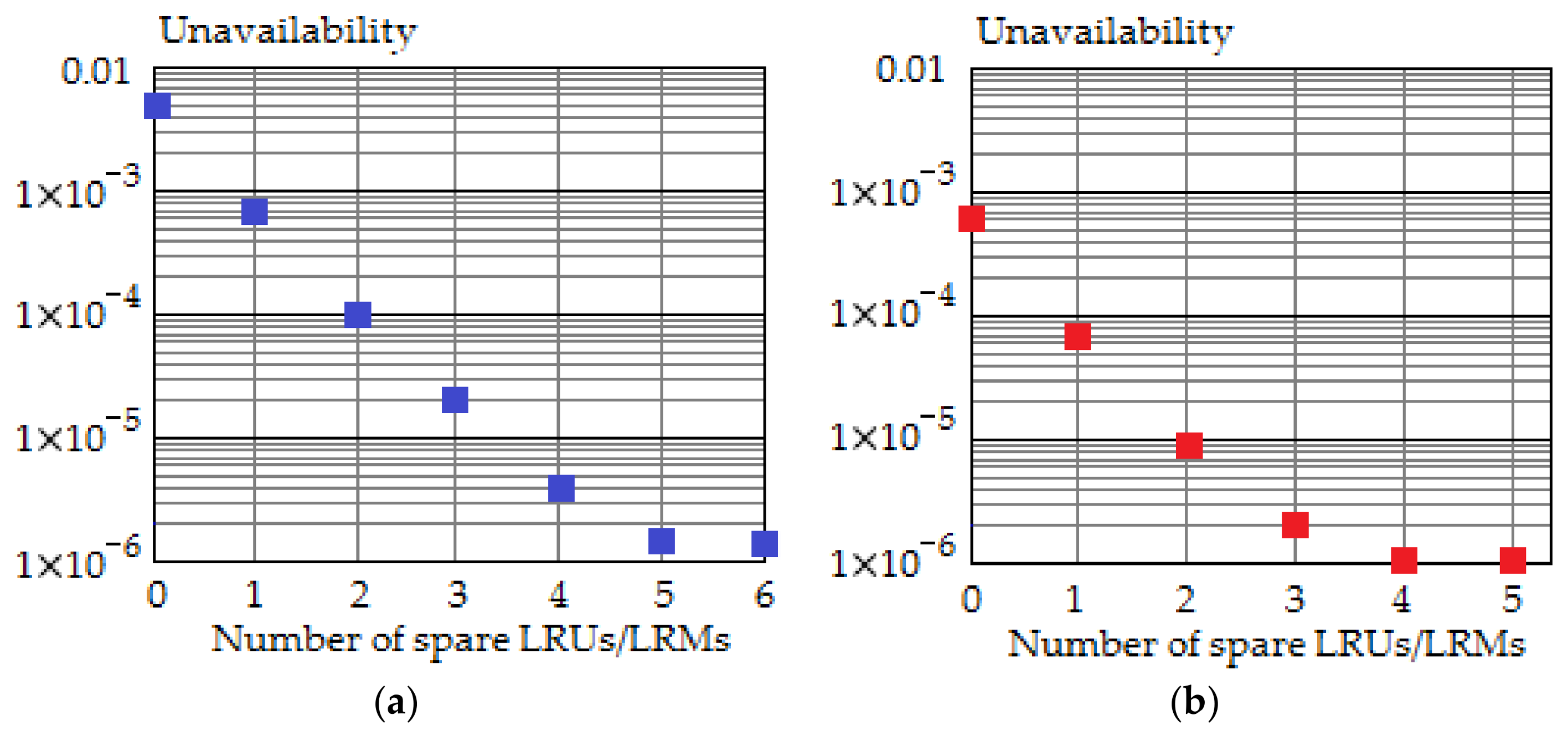
Figure 3a shows the dependence of unavailability of the duplicated avionics system on the number of spare LRUs/LRMs (r) in the airline’s warehouse for the case of 20 aircraft when , , and .
As can be seen from Figure 3a, the unavailability decreases by a factor of 3300 with an increase in the number of spare LRUs/LRMs from 0 to 5, and at the unavailability reaches constant value. Therefore, any further increase in the number of spare LRUs/LRMs is not practical.
Figure 3b shows the dependence of the unavailability on the number of spare LRUs/LRMs for the case when the rate of intermittent faults is zero. As can be seen from Figure 3b, with η = 0, the unavailability reaches a constant value with less number of spare LRUs/LRMs than when . Thus, intermittent faults lead to an increase in the number of spare LRUs/LRMs necessary to provide the required value of the unavailability for the redundant avionics systems.
2.4. Mean Time between Unscheduled Removals
One of the most important indicators of the maintenance effectiveness is the MTBUR of avionics LRU/LRM. According to [34], the MTBUR is close to 50% of the mean time between failures (MTBF). The main reason for this decrease in the MTBUR compared to the MTBF is a rather high rate of unconfirmed failures and especially intermittent faults. Let us derive the MTBUR equation for the avionics LRU/LRM.
Assume, as in Section 2.2, that the LRU/LRM permanent failure occurs at time υ, where . Then, the LRU/LRM will be removed from the aircraft board at time , if an intermittent fault occurs during -th flight, where . Further, the LRU/LRM will be removed from the aircraft board at time , if till time there is no intermittent fault. Therefore, under the condition that , the mathematical expectation of the time to the LRM/LRU removal is equal to
Applying to (19) the formula of complete mathematical expectation, we get
Substituting exponential PDFs and into (20), we obtain
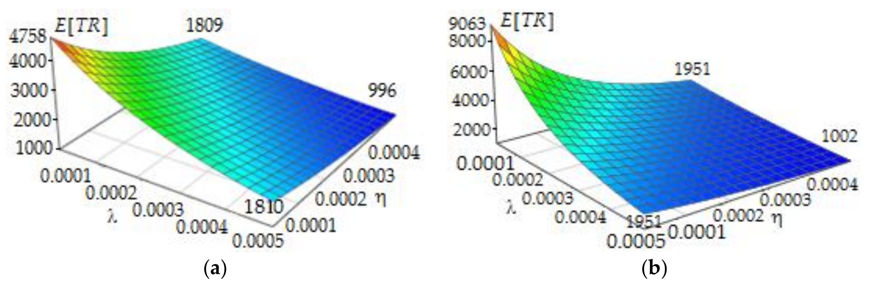
In Figure 4a,b, 3D plots of the MTBUR dependence on the rates of permanent failures and intermittent faults are shown for different values of T. As can be seen from Figure 4, MTBUR decreases when λ and η increase. It should be also noted that MTBUR depends strongly on T for small values of the rate of permanent failures and intermittent faults. For large values of λ and η, MTBUR almost does not depend on T.
2.5. Expected Total Maintenance Cost
The expected total maintenance cost (ETMC) depends on the chosen maintenance option during warranty or post-warranty period. For definiteness, we will consider post-warranty period. The ETMC of avionics LRUs/LRMs for κ-th maintenance option can be represented as follows:
where n is the number of identical LRUs/LRMs in the avionics system, M is the number of aircraft in the airline, is the average cost of one unscheduled removal of the LRU/LRM and further repair for the κ-th maintenance option, is the mathematical expectation of the LRU/LRM removals in the interval (0, T), and is the capital expenditures required to organize the κ-th maintenance option.
The mathematical expectation of the LRU/LRM removals in the interval (0, T) can be expressed through the MTBUR and T as follows:
Let us consider possible maintenance options during the post warranty period. Small or budget airlines may not have enough money to organize O-, I- and D-level maintenance. Therefore, some of these airlines may use only O-level maintenance. In this case κ = 1 and cost function is given by
where is the average cost of the O-level maintenance, is the average cost of repairing the LRU/LRM outside the airline, i.e., in a repair station or at the manufacturer, is the average cost of shipping the LRU/LRM to the repair and back to the warehouse.
For this option of maintenance, capital expenditures include only the cost of spare LRUs/LRMs used in the O-level maintenance. Therefore,
where is the number of spare LRUs/LRMs in the airline warehouse and is the cost of one spare LRU/LRM.
Let us now consider the second (κ = 2) maintenance option, which includes O- and I-Level maintenance. The third maintenance level is outsourced. At the I-level maintenance ATE is usually used to test the suspicious LRUs/LRMs and detect the faulty SRUs. Traditional ATE cannot diagnose intermittent faults in dismantled LRUs/LRMs for a variety of reasons [9]. Intermittent faults registered on-board cannot be confirmed by ATE in this maintenance option. Therefore, only SRUs with permanent failures are shipped to the manufacturer or repair station for repairing. The spare parts in this maintenance option are LRUs/LRMs and SRUs.
The average repair cost of the LRU/LRM for the κ = 2 maintenance option is determined as follows:
where is the average cost of I-level maintenance, is the average cost of shipping the SRU to the place of repair and back to the airline warehouse, is the average cost of the SRU repair at the manufacturer or repair station, and is the a posteriori probability that the dismantled LRM/LRU has a permanent failure.
The a posteriori probabilities that the LRU/LRM removed from the aircraft board had an intermittent fault or a permanent failure are expressed through the mean times and as follows:
Capital expenditures include the cost of spare LRUs/LRMs used in the O-level maintenance, the cost of spare SRUs used in the I-level maintenance, and the relative cost of ATE, i.e.,
where is the cost of the l-th type of spare SRU, is the number of spare SRUs of the l-th type, is the cost of ATE, which is used at the I-level, and W is the number of different LRUs/LRMs that ATE can test at the I-level.
Let us consider one of the possible options to implement a three-level maintenance system, including O-, I-, and D-levels. As already noted, maintenance at the D-level is carried out in the specialized repair shops equipped with diagnostic tools capable of detecting a failed non-recoverable electronic component or a group of components in the SRU that is rejected at the I-level. The spare parts at this maintenance level are assemblies and electronic components. Due to the disadvantages of traditional ATE in detecting intermittent faults, specialized intermittent fault detector (IFD) and intermittent fault detection and isolation system (IFDIS) have recently been developed [35,36]. IFD and IFDS can be used as in the I-level as well as in the D-level maintenance.
The average repair cost of the LRU/LRM for the κ = 3 maintenance option is determined as follows:
where and are, respectively, the average cost of the I-level maintenance for an LRU/LRM with a permanent failure and intermittent fault, and are, respectively, the average cost of the D-level maintenance for an SRU with a permanent failure and intermittent fault.
Capital expenditures include the cost of spare LRUs/LRMs used in the O-level, the cost of spare SRUs used in the I-level, the cost of spare assemblies and electronic components used in the D-level, the relative cost of ATE used in the I-level, the relative cost of IFD used in the I- and D-level, and the cost of repair tools used in the D-level maintenance. So,
where is the cost of spare parts in the D-level maintenance, is the cost of IFD, and is the cost of repair tools used in the D-level maintenance.
3. Results
In this section, we consider an example of using the mathematical model developed in Section 2 to choose the best maintenance option for a redundant avionics system.
Let us calculate the ETMC for the air data inertial reference system (ADIRS). The ADIRS provides traffic data (airspeed, angle of attack and altitude) and information on inertial control (position and altitude) on the displays to pilots, as well as to other aircraft systems such as engines, autopilot, flight control system and chassis. The ADIRS consists of fault-tolerant air data inertial reference units (ADIRUs) located in the aircraft electronics rack. Typical ADIRU comprises the following SRUs: an air data computer, multimode receiver, 3 digital ring laser gyros, 3 quartz accelerometers, and power supply module.
The following data are used in calculation of the ETMC for different maintenance options: , , , , , , , , , , , 1000$, , , , , , , , , , , and .
The results of calculation are shown in Table 1. Since in the third option of maintenance the IFD is used, the rate of intermittent faults in repaired ADIRUs should be significantly reduced. As described in [37], after repairing the AN/APG-68 airborne radar of the F-16 using IFDIS, MTBUR increased more than threefold. Therefore, it was assumed in the calculations that for the third maintenance option, the rate of intermittent faults is 3 times less, i.e., To determine the optimal number of spare ADIRUs, a mathematical model for the operation of the warehouse of spare LRUs based on Markov chains with continuous time was developed. The optimum number of spare LRUs ensured the absence of delays in scheduled flights of aircraft.
The number of spare SRUs was calculated for confidence probability of 0.99 for each type of SRU. According to the calculations, in the second maintenance option there should be two spare SRUs of each type in the warehouse, and in the second maintenance option only one spare SRU.
As can be seen from Table 1, the third maintenance option, which uses IFD at the I- and D-level maintenance, has the lowest maintenance cost and is therefore the best. Indeed, the maintenance cost in the third maintenance option is 8.3 times smaller than in the first option and more than 3.5 times smaller than for the second option.
It should also be noted that the unavailability of ADIRS is the same for all maintenance options. This means that unavailability (or availability) of the redundant avionics systems cannot be used to select the best maintenance option of avionics systems because it does not depend on the characteristics of the I- and D-level maintenance.
The results of Table 1 convincingly show the preference of using the third maintenance option in airlines. The question of the stability of the obtained results to the change in the rate of intermittent faults is also topical. Figure 5 shows the dependence of ETMC on the rate of intermittent faults for each maintenance option. As can be seen in Figure 5, the first maintenance option is very sensitive to the rate of intermittent faults, since EMTC is increased from $ to $ (i.e., almost 28 times increase) when η is changed from to . However, when using the third maintenance option and the same change in the rate of intermittent faults, the ETMC increases from $ to $, i.е., only four times increase. The second maintenance option also has the stability to the change of the intermittent fault rate, however, when using it, the ETMC is 2–3 times greater than in the third option.
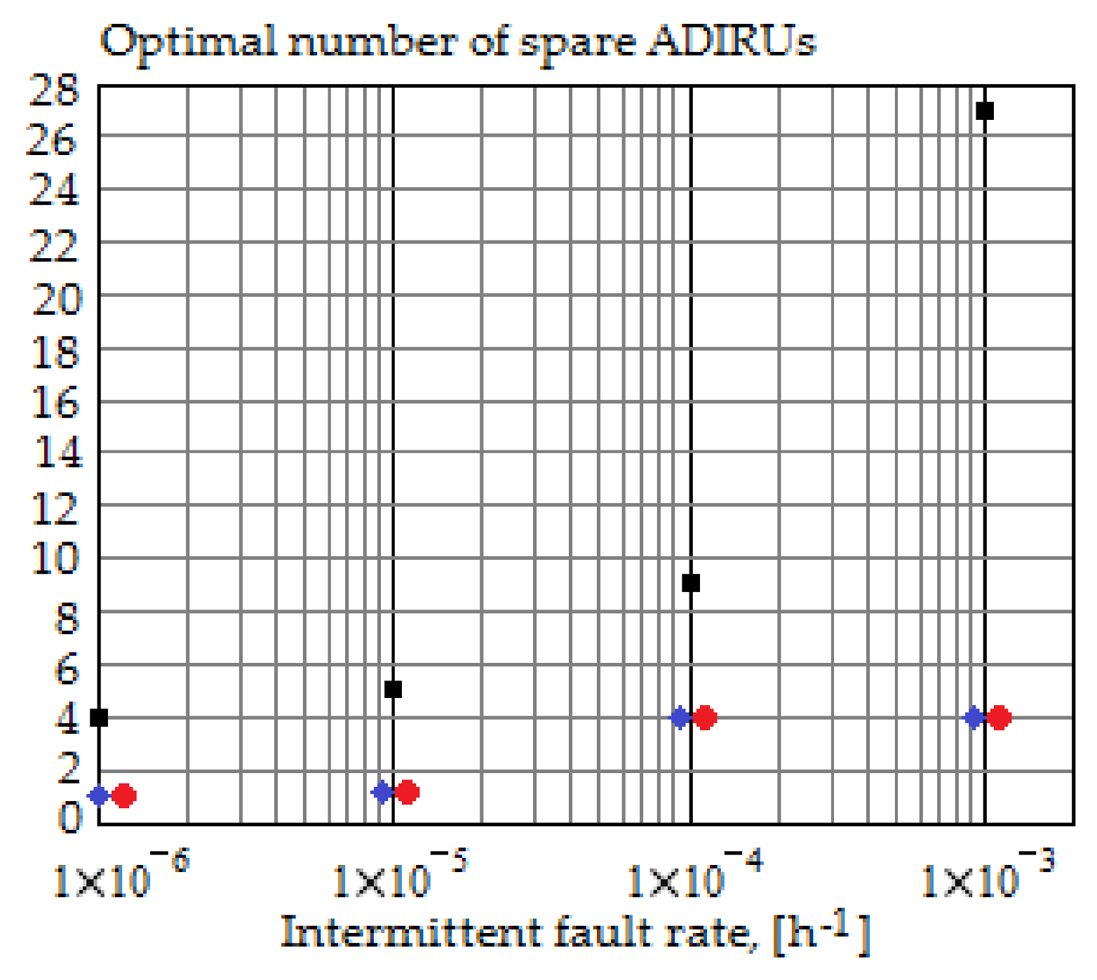
Figure 6 shows the dependence of the optimal number of spare ADIRUs on the rate of intermittent faults for the first, second, and third maintenance options.
As can be seen from Figure 6, first, to ensure the regularity of flights, a significantly larger number of spare ADIRUs is required for the first maintenance option compared to the second and third options and, second, the optimal number of spare ADIRUs is very strongly depends on the rate of intermittent faults for the first maintenance option and weakly depends for the second and third options.
4. Discussion
In this study, a mathematical model has been developed to evaluate the availability and expected maintenance cost of continuously tested LRMs/LRUs and redundant avionics systems over a finite interval of time, taking into account the effect of both permanent failures and intermittent faults. Unlike most published studies, such as [20,21,22,23,24,25], the developed mathematical model considers the specifics of the architecture and application of modern avionics systems and can be used for any law of distribution of the operating time to permanent failure and intermittent fault. The described model might be further developed in order to divide the NFF events to intermittent faults and false alarms of the BITE. The need for separate consideration of false alarms is due to the fact that the level of false alarms is high enough in the aviation industry, reaching 28% of all events associated with alarm signals [38].
A number of publications point to the topical need for a cost assessment of the consequences of NFF events in electronic systems [12,17]. This problem is indeed topical because according to [39], the average cost of losses due to NFF per aircraft in the US civil aviation was about $200,000 in 2013. Similar losses exist in military aviation [40,41]. So, according to the US Department of Defense, three out of four (75%) weapon systems are subject to NFF-type failures [41]. NFF costs the US Department of Defense $2 billion to $10 billion in losses per year [8]. As indicated in [8,9], the main cause of NFF events are the intermittent faults that occur in flight. Therefore, the developed mathematical model for evaluating the average cost of avionics systems maintenance with taking into account the effect of intermittent faults is of undoubted interest for developers of maintenance programs for avionics systems of civil and military aircraft. The proposed cost model allows not only to assess the impact of intermittent faults, but also to choose the maintenance option that is practically independent on the rate of intermittent faults, thus ensuring the minimum cost of maintenance. The ideas in this paper are illustrated by an example that describes three maintenance options for the redundant avionics system ADIRS. Among these maintenance options, the option of a three-level maintenance with IFD at the second and third maintenance levels is of particular interest. Despite additional capital expenditures, this option provides the lowest average maintenance cost, which is 8.3 times less than in a single-level and 3.5 times less than in a two-level maintenance system without using IFD. This result is explained by the fact that the application of the IFD allows the identification of SRUs with intermittent faults at the I-level maintenance and, subsequently, at the D-level maintenance to eliminate the causes of such faults. At the same time the rate of intermittent faults decreases and, hence, the MTBUR increases. The performed calculations fully confirm the statistical data given in [37].
Future research directions may include the development of cost models for maintenance options with different combinations of O-, I-, and D-levels of maintenance with the involvement of outsourcing service companies.
5. Conclusions
This study has focused on developing a maintenance model of digital avionics systems. The proposed mathematical model can be used for both federated and integrated modular avionics architecture of modern aircraft. The derived analytical expressions for the calculation of the availability, MTBUR and expected total maintenance cost can be used for any law of time distribution to permanent failure and intermittent fault, including both cases of sudden failures and faults and cases of gradual failures and faults, which are typical for deteriorating systems. Since many avionics systems have an exponential time-to-failure distribution, the mathematical expressions have been derived to calculate the mean times spent by the LRU/LRM in different operation and maintenance states for the case of an exponential distribution of the operating time to permanent failure and intermittent fault. On illustrative numerical examples it has been shown that the average availability of the LRU/LRM and redundant avionics system begins to decrease significantly when the rate of intermittent faults is greater than and MTBUR decreases five times with increasing the rate of intermittent faults from to . It has also been shown that the presence of the intermittent faults increases the number of spare LRUs/LRMs required to ensure the regularity of flights. Thus, numerical results obtained on the basis of the proposed maintenance model confirm statistical data on the consequences of unconfirmed failures [10,11,12]. The generalized equations have been developed to calculate the expected total maintenance cost during finite horizon of operation for three alternative maintenance options that differ by existence of I- and D-levels of maintenance; the numerical example shows that a three-level post-warranty maintenance system is optimal for the selected source data, since it results in a minimum number of spare LRUs and SRUs, as well as minimum operating costs being 8.3 times less than for a single-level system and 3.5 times less than in a two-level maintenance system. The practical significance of the obtained results is that the proposed maintenance models allow one to compare the various options for organizing the maintenance of avionics and to choose the option that provides the lowest cost of maintenance. As shown by numerical calculations, the cost of different maintenance options can differ by several times, which cannot be predicted in the absence of the proposed mathematical models.
Conflicts of Interest
The authors declare no conflict of interest.
References
- Bieber, P.; Boniol, F.; Boyer, M. New challenges for future avionic architectures. AerospaceLab 2012, 4, 1–10. [Google Scholar]
- Gaska, T.; Watkin, C.; Chen, Y. Integrated modular avionics—Past, present, and future. IEEE Aerosp. Electron. Syst. Mag. 2015, 30, 12–23. [Google Scholar] [CrossRef]
- Alena, R.L.; Ossenfort, J.; Laws, K.I. Communications for integrated modular avionics. In Proceedings of the 2007 IEEE Aerospace Conference, Big Sky, MT, USA, 3–10 March 2007. [Google Scholar]
- Module 11.19 integrated modular avionics (ATA 42). AFAQ Inst. Aviat. Technol. 2012, 2, 1–64.
- A380 Technical Training Manual. LEVEL I—ATA 42 Integrated Modular Avionics & Avionics Data Communication Network; Airbus: Toulouse, France, 2006; pp. 1–20.
- ARINC Specification 825: General Standardization of CAN (Controller Area Network) Bus Protocol for Airborne Use. Available online: http://www.arinc-825.com/arinc825-standard (accessed on 1 July 2015).
- Syed, W.A.; Khan, S.; Phillips, P.; Perinpanayagam, S. Intermittent fault finding strategies. Procedia CIRP 2013, 11, 74–79. [Google Scholar] [CrossRef]
- Anderson, K. Intermittent Fault Detection and Isolation Reduces NFF and Enables Cost Effective Readiness. Available online: http://www.ncms.org/wp-content/uploads/3-Steadman-CTMA-Briefing-2017.pdf (accessed on 4 April 2017).
- Steadman, B.; Berghout, F.; Olsen, N. Intermittent fault detection and isolation system. In Proceedings of the 2008 IEEE AUTOTESCON, Salt Lake City, UT, USA, 8–11 September 2008; pp. 37–40. [Google Scholar]
- Soderholm, P. A system view of the no fault found (NFF) phenomenon. Reliab. Eng. Syst. Saf. 2007, 92, 1–14. [Google Scholar] [CrossRef]
- Hockley, C.; Phillips, P. The impact of no fault found on through-life engineering services. J. Qual. Maint. Eng. 2012, 18, 141–153. [Google Scholar] [CrossRef]
- Khan, S.; Phillips, P.; Jennions, I.; Hockley, C. No Fault Found events in maintenance engineering Part 1: Current trends, implications and organizational practices. Reliab. Eng. Syst. Saf. 2014, 123, 183–195. [Google Scholar] [CrossRef] [Green Version]
- Sandborn, P.; Feldman, K.L.; Ghelam, S. Life cycle cost impact of using prognostic health management (PHM) for helicopter avionics. Microelectron. Reliab. 2007, 47, 1857–1864. [Google Scholar]
- Ulansky, V.V.; Machalin, I.A. Optimization of post warranty maintenance of avionics systems. In Proceedings of the 2007 International Conference on Aeronautical Science and Air Transportation (ICASAT2007), Tripoli, Libya, 23–25 April 2007; pp. 619–628. [Google Scholar]
- Curry, E.E. FALCCM-H: Functional avionics life cycle model for hardware. In Proceedings of the 1993 IEEE National Aerospace and Electronics Conference (NAECON 1993), Dayton, OH, USA, 24–28 May 1993; Volume 2, pp. 950–953. [Google Scholar]
- Ilarslan, M.; Ungar, L.Y.; Ilarslan, K. An economic analysis of false alarms and no fault found events in air vehicles. In Proceedings of the 2016 IEEE AUTOTESTCON, Anaheim, CA, USA, 12–15 September 2016; pp. 1–7. [Google Scholar]
- Erkoyuncu, J.A.; Khan, S.; Hussain, S.M.; Roy, R. A framework to estimate the cost of no-fault found events. Int. J. Prod. Econ. 2016, 173, 207–222. [Google Scholar] [CrossRef] [Green Version]
- Ulansky, V.; Terentyeva, I. Availability modeling of a digital electronic system with intermittent failures and continuous testing. Eng. Lett. 2017, 25, 104–111. [Google Scholar]
- Vega, D.J.G.; Pamplona, D.A.; Oliveira, A.V.M. Assessing the influence of the scale of operations on maintenance costs in the airline industry. J. Trans. Lit. 2016, 10, 10–14. [Google Scholar] [CrossRef]
- Nakagava, Т. Maintenance Theory of Reliability; Springer: London, UK, 2005; pp. 220–224. [Google Scholar]
- Hsu, Y.T.; Hsu, C.F. Novel model of intermittent faults for reliability and safety measures in long-life computer systems. Int. J. Electron. 1991, 71, 917–937. [Google Scholar] [CrossRef]
- Kranitis, N.; Merentitis, A.; Laoutaris, N. Optimal periodic testing of intermittent faults in embedded pipeline processor applications. In Proceedings of the 2006 Design, Automation and Test in Europe Conference, Munich, Germany, 6–10 March 2006; pp. 65–70. [Google Scholar]
- Prasad, V.B. Digital systems with intermittent faults and Markovian models. In Proceedings of the 1992 IEEE 35th Midwest Symposium on Circuits and Systems, Washington, DC, USA, 9–12 August 1992; pp. 195–198. [Google Scholar]
- Zhao, X.; Chen, M.; Nakagawa, T. Optimal time and random inspection policies for computer systems. Appl. Math. Inf. Sci. 2014, 8, 413–417. [Google Scholar]
- Rashid, L.; Pattabiraman, K.; Gopalakrishnan, S. Intermittent hardware errors recovery: Modeling and evaluation. In Proceedings of the 2012 Ninth International Conference on Quantitative Evaluation of Systems (QEST), London, UK, 17–20 September 2012; pp. 1–10. [Google Scholar] [CrossRef]
- Raza, A.; Ulansky, V. Assessing the impact of intermittent failures on the cost of digital avionics’ maintenance. In Proceedings of the 2016 IEEE Aerospace Conference, Big Sky, MT, USA, 5–12 March 2016; pp. 1–16. [Google Scholar]
- Raza, A.; Ulansky, V. Minimizing total lifecycle expected costs of digital avionics’ maintenance. Procedia CIRP 2015, 38, 118–123. [Google Scholar] [CrossRef]
- MIL-HDBK-338B. In Military Handbook; Electronic Reliability Design Handbook; Department of Defense: Arlington County, VA, USA, 1998; pp. 5.72–5.74.
- Elsayed, E.A. Reliability Engineering, 2nd ed.; Wiley: Hoboken, NJ, USA, 2012; pp. 198–206. [Google Scholar]
- Drenick, R.F. The failure law of complex equipment. J. Soc. Ind. Appl. Math. 1960, 8, 680–690. [Google Scholar] [CrossRef]
- Qin, J.; Huang, B.; Walter, J. Reliability analysis in the commercial aerospace industry. J. Reliab. Anal. Center 2005, 1, 1–5. [Google Scholar]
- Yeh, Y.C. Safety critical avionics for the 777 primary flight controls system. In Proceedings of the 2001 IEEE Digital Avionics Systems Conference (DASC), Daytona Beach, FL, USA, 14–18 October 2001; pp. 1–9. [Google Scholar]
- Rausand, M.; Hoyland, A. System Reliability Theory: Models, Statistical Methods, and Applications, 2nd ed.; Wiley: New York, NY, USA, 2003; pp. 147–152. [Google Scholar]
- Kayton, M.; Fried, W.R. Avionics Navigation Systems, 2nd ed.; Wiley: New York, NY, USA, 1997; p. 700. [Google Scholar]
- Voyager Intermittent Fault Detector (VIFDT). Available online: http://www.usynaptics.com/index.php/products/ncompass-voyager (accessed on 1 January 2017).
- Intermittent Fault Detection & Isolation System (IFDS). Available online: http://www.usynaptics.com/index.php/products/ifdis (accessed on 1 January 2017).
- Anderson, K. IFDIS—Expanding role across the DoD maintenance enterprise. In Proceedings of the 2012 Department of Defense Maintenance Symposium, Grand Rapids, MI, USA, 13–16 November 2012; pp. 1–29. [Google Scholar]
- Bliss, J.P. Investigation of alarm-related accidents and incidents in aviation. Int. J. Aviat. Psychol. 2003, 13, 249–268. [Google Scholar] [CrossRef]
- NFF—No Fault Found. American Institute of Aeronautics and Astronautics. Available online: https://info.aiaa.org/tac/AASG/PSTC/Lists/Calendar/Attachments/1/NFF%20Subcommittee.pdf (accessed on 22 April 2013).
- Hockley, C.; Laceya, L. A research study of no fault found (NFF) in the Royal Air Force. Procedia CIRP 2017, 59, 263–267. [Google Scholar] [CrossRef]
- Hockley, C.J.; Lacey, L.; Pelham, J.G. Report for Air Command on the Impact of no Fault Found (NFF) on a Selection of RAF Aircraft Fleets; Technical Report TES 02-01-2015; EPSRC Through-Life Engineering Services Centre, Cranfield University: Bedford, UK, 2015. [Google Scholar]
Figure 1.
(a) A 3D plot of the dependence of the line replaceable unit (LRU)/line replaceable module (LRM) availability on the rates of permanent failures and intermittent faults when and ; (b) A 3D plot of the dependence of the LRU/LRM availability on the rates of permanent failures and intermittent faults when and .
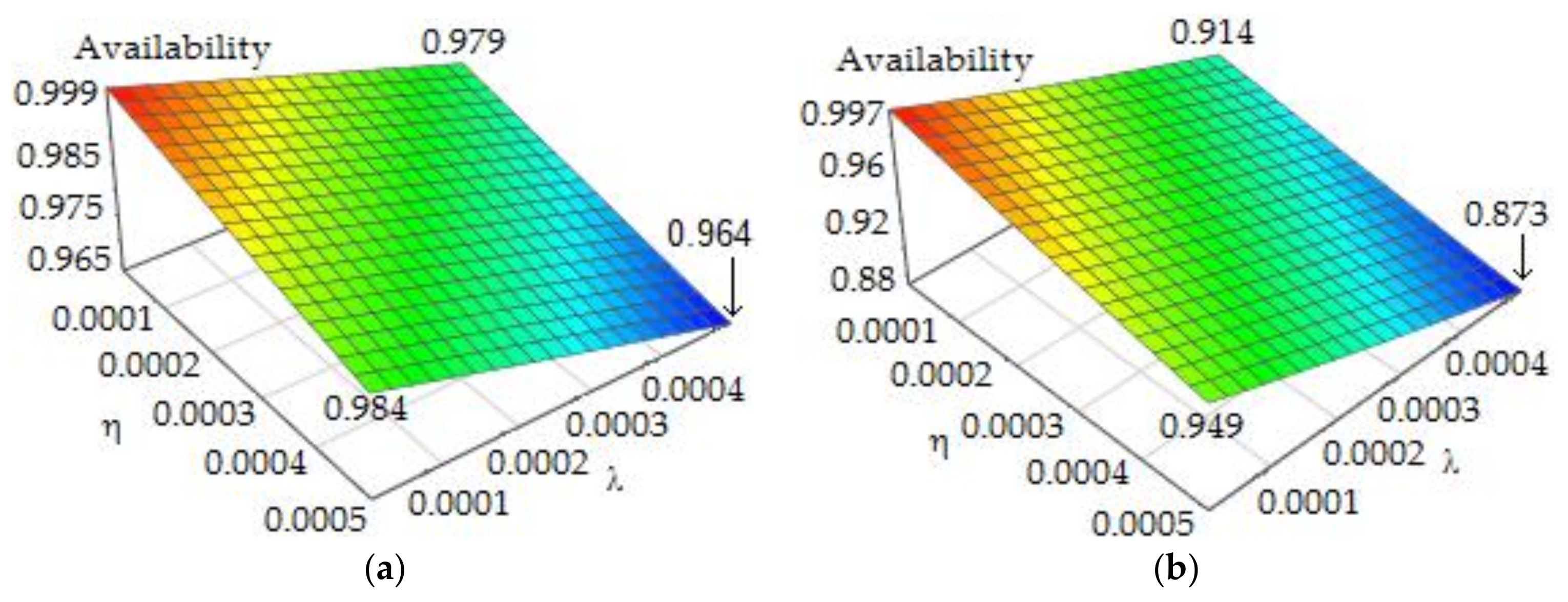
Figure 2.
(a) Dependence of unavailability of the duplicated avionics system on the rate of intermittent faults when λ = 2 × 10⁻⁴ h−1; (b) Dependence of unavailability of the duplicated avionics system on the rate of permanent failures when η = 2 × 10⁻⁴ h−1.
Figure 2.
(a) Dependence of unavailability of the duplicated avionics system on the rate of intermittent faults when λ = 2 × 10⁻⁴ h−1; (b) Dependence of unavailability of the duplicated avionics system on the rate of permanent failures when η = 2 × 10⁻⁴ h−1.

Figure 3.
(a) Dependence of unavailability of the duplicated avionics system on the number of spare LRUs/LRMs when λ = η = 2 × 10⁻⁴ h−1; (b) Dependence of unavailability of the duplicated avionics system on the number of spare LRUs/LRMs when λ = 2 × 10⁻⁴ h−1 and η = 0.
Figure 3.
(a) Dependence of unavailability of the duplicated avionics system on the number of spare LRUs/LRMs when λ = η = 2 × 10⁻⁴ h−1; (b) Dependence of unavailability of the duplicated avionics system on the number of spare LRUs/LRMs when λ = 2 × 10⁻⁴ h−1 and η = 0.

Figure 4.
(a) A 3D plot of the dependence of the mean time between unscheduled removals (MTBUR) on the rates of permanent failures and intermittent faults when ; (b) A 3D plot of the dependence of the MTBUR on the rates of permanent failures and intermittent faults when .
Figure 4.
(a) A 3D plot of the dependence of the mean time between unscheduled removals (MTBUR) on the rates of permanent failures and intermittent faults when ; (b) A 3D plot of the dependence of the MTBUR on the rates of permanent failures and intermittent faults when .

Figure 5.
Expected total maintenance cost as a function of the intermittent fault rate for the first maintenance option (black squares), second maintenance option (blue rhombus), and third maintenance option (red circles).
Figure 5.
Expected total maintenance cost as a function of the intermittent fault rate for the first maintenance option (black squares), second maintenance option (blue rhombus), and third maintenance option (red circles).
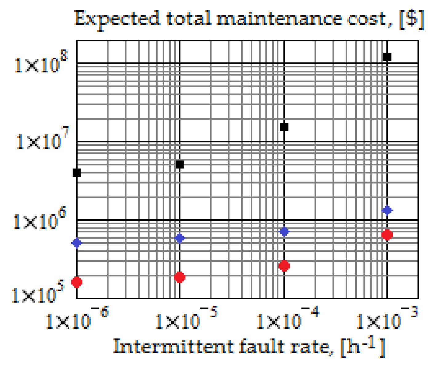
Figure 6.
Optimal number of spare ADIRUs as a function of the intermittent fault rate for the first maintenance option (black squares), second maintenance option (blue rhombus), and third maintenance option (red circles).
Figure 6.
Optimal number of spare ADIRUs as a function of the intermittent fault rate for the first maintenance option (black squares), second maintenance option (blue rhombus), and third maintenance option (red circles).

Table 1.
Calculation results for three options of air data inertial reference system (ADIRS) maintenance.
Table 1.
Calculation results for three options of air data inertial reference system (ADIRS) maintenance.
| Maintenance Option (κ) | MTBUR of ADIRU (h) | Optimal Number of Spare ADIRU | Optimal Number of Spare SRU | Expected Maintenance Cost ($) | Unavailability of ADIRS |
|---|---|---|---|---|---|
| κ = 1 | 20,690 | 4 | 0 | ||
| κ = 2 | 20,690 | 1 | 2 | ||
| κ = 3 | 25,410 | 1 | 1 |
© 2018 by the author. Licensee MDPI, Basel, Switzerland. This article is an open access article distributed under the terms and conditions of the Creative Commons Attribution (CC BY) license (http://creativecommons.org/licenses/by/4.0/).
Share and Cite
MDPI and ACS Style
Raza, A. Maintenance Model of Digital Avionics. Aerospace 2018, 5, 38. https://doi.org/10.3390/aerospace5020038
AMA Style
Raza A. Maintenance Model of Digital Avionics. Aerospace. 2018; 5(2):38. https://doi.org/10.3390/aerospace5020038
Chicago/Turabian StyleRaza, Ahmed. 2018. "Maintenance Model of Digital Avionics" Aerospace 5, no. 2: 38. https://doi.org/10.3390/aerospace5020038
Note that from the first issue of 2016, this journal uses article numbers instead of page numbers. See further details here.