Influence of Nozzle Exit Conditions on the Near-Field Development of High Subsonic and Underexpanded Axisymmetric Jets

1
Department of Aero & Auto Engineering, Loughborough University, Loughborough LE11 3TU, UK
2
Rolls-Royce Deutschland, Eschenweg 11, Dahlewitz, 15827 Blankenfelde-Mahlow, Germany
*
Author to whom correspondence should be addressed.
Aerospace 2018, 5(2), 35; https://doi.org/10.3390/aerospace5020035
Submission received: 19 February 2018
/
Revised: 17 March 2018
/
Accepted: 19 March 2018
/
Published: 29 March 2018
(This article belongs to the Special Issue Under-Expanded Jets)
Abstract
:Detailed knowledge of jet plume development in the near-field (the first 10–15 nozzle exit diameters for a round jet) is important in aero-engine propulsion system design, e.g., for jet noise and plume infrared (IR) signature assessment. Nozzle exit Mach numbers are often high subsonic but improperly expanded (e.g., shock-containing) plumes also occur; high Reynolds numbers (O (106)) are typical. The near-field is obviously influenced by nozzle exit conditions (velocity/turbulence profiles) so knowledge of exit boundary layer characteristics is desirable. Therefore, an experimental study was carried out to provide detailed data on nozzle inlet and exit conditions and near-field development for convergent round nozzles operated at Nozzle Pressure Ratios (NPRs) corresponding to high subsonic and supersonic (underexpanded) jet plumes. Both pneumatic probe and Laser Doppler Anemometry (LDA) measurements were made. The data revealed that internal nozzle acceleration led to a dramatic reduction in wall boundary layer thickness and a more laminar-like profile shape. The addition of a parallel wall extension to the end of the nozzle allowed the boundary layer to return to a turbulent state, increasing its thickness, and removing vena contracta effects. Differences in nozzle exit boundary layers exerted a noticeable influence but only in the first few diameters of plume development. The addition of the exit extension removed the vena contracta effects of the convergence only design. At underexpanded NPRs, this change to nozzle geometry modified the shock cell pattern and shortened the potential core length of the jet.
1. Introduction
Aero-engine manufacturers require a detailed understanding of propulsion jet flow characteristics for both civil and military applications, driven by design objectives of low jet noise (civil) and a reduced infrared (IR) signature (military). In this context, it is jet/ambient near-field mixing which is primarily of interest (i.e., approximately the first 10–15 nozzle exit diameters) rather than the far-field, where jet development is observed to obey self-similarity laws. This increases the technical challenge considerably because developing near-field turbulence is more complex. After nozzle exit, the nozzle wall boundary layer is transformed into a free shear layer, a process clearly influenced by nozzle exit conditions. Accordingly, internal nozzle flow development is also influential. Near-field jet aerodynamic and aeroacoustic characteristics depend strongly on the near-field turbulent structures which control temperature reduction in hot jets and are the primary source of broadband noise in subsonic jets.
The work described in G. Papadopolous et al. [1] was one of the first to present measurements in incompressible jets, demonstrating that nozzle exit conditions are important in the development of the initial shear layer, the potential core length, and the transition to self-similarity. Jet Mach numbers are high subsonic or supersonic. Accordingly, the initial jet Mach number (MJ) (equivalent to the operating Nozzle Pressure Ratio (NPR)) and associated compressibility effects will play a role. Other factors which influence near-field development are the jet Reynolds number (ReJ), the jet initial temperature (or density), and the state and thickness of the nozzle exit boundary layer. For NPRs above critical (1.893 for air) supersonic improperly expanded jets occur. If attention is restricted to convergent-only nozzles, when NPR exceeds the critical or choked flow value, the static pressure at nozzle exit is greater than ambient (i.e., underexpanded flow). Adjustment of this pressure mismatch takes place via a series of expansion and compression waves which create the appearance of shock-cells (‘shock diamonds’) in the jet plume until pressure equilibrium is reached. The present study considers only convergent round nozzle geometries and jet total temperatures equal to ambient but all other factors influencing near-field development are addressed.
Typical propulsion nozzle Reynolds numbers (ReJ = ρJUJD/μJ), where UJ and D are nozzle exit bulk velocity and diameter, are ~106. P. Bradshaw [2] suggested that, at such high values of ReJ, self-similar jet flow becomes independent of the nozzle Reynolds number. The data in F.P. Ricou and D.B. Spalding [3] and W.M. Pitts [4] supported this, showing no influence on the rate of entrainment into the jet above Reynolds numbers of 25,000 [3] and 50,000 [4] respectively. P. Bradshaw [2] also argued that even near-field effects of ReJ are essentially exerted through the indirect effect of Reynolds number on the nozzle wall boundary layer development, which sets conditions at the nozzle exit lip. This was later confirmed by measurements reported in G. Xu and R.A. Antonia [5]. The present study conducts measurements at ReJ values of order 106 and it is not believed there is any direct influence of ReJ on the data reported.
The compressibility effects which accompany high NPR/high jet Mach number occur predominantly in the shear layer emanating from the nozzle lip. D. Papamoschou and A. Roshko [6] was the first to provide experimental evidence of the significant reduction in two-dimensional (planar) shear layer growth rate due to compressibility effects. This correlated to the convective Mach number (MC), which represents the Mach number in a frame of reference moving with the speed of shear layer instability waves or disturbances such as turbulent structures. MC for two-stream mixing where both streams have the same specific heat ratio is defined as:
U and a are the flow speed and speed of sound respectively and subscripts 1 and 2 indicate the faster/slower streams. A curve fit to the planar shear layer data showed that the shear layer growth rate decreased rapidly with MC, reaching a value of just 20% of the equivalent incompressible shear layer at MC = 1. The same experiment has been repeated by many authors with similar results; a recent re-examination in M.F. Barone et al. [7] of 11 sets of experimental data produced what is now considered the standard curve for the decrease of compressible planar mixing layer spread rate with increasing MC. This has been used to introduce compressibility corrections into several Reynolds Averaged Navier Stokes (RANS) turbulence models (see S. Sarkar and B. Lakshmanan [8]). For a jet discharged into a stagnant ambient, D.A. Yoder et al. [9] noted that when MJ exceeds 0.5 then MC across the nozzle shear layer is high enough for compressibility effects to be significant, leading to potential core lengths greater than observed for incompressible jets.
Although D. Papamoschou and A. Roshko [6] studied 2D planar shear layers, the first experimental measurements confirming that similar behaviour occurred in axisymmetric (two-dimensional annular) shear layers, as in the round jet near-field, were described by J.C. Lau [10,11]. Subsonic and perfectly expanded supersonic jets with nozzle exit Mach numbers from 0.3 to 1.7 were studied and the potential core length was shown to increase with . Work on axisymmetric jets was recently extended by T. Feng and J.J. McGuirk [12] to consider moderately underexpanded NPRs. The annular shear layer data of J.C. Lau and T. Feng and J.J. McGuirk [10,11,12] were all in agreement, but did not collapse onto the best-fit curve of planar data provided in M.F. Barone et al. [7]. Compressibility effects in annular shear layers began at a lower MC and displayed stronger reduction in shear layer spread rate than for planar shear layers at the same MC, implying this effect is very important for compressible jet near-field development.
The final factor controlling near-field development to consider is the state and profile characteristics of the nozzle exit boundary layer. Considerable work has been published in this area, although little has direct relevance to the present application. Many studies have only examined too low nozzle Reynolds and Mach numbers or concentrated on exit profiles which are far removed from the operating conditions relevant to aero-propulsion (e.g., purely laminar boundary layers or fully developed turbulent pipe flow profiles). This can lead to misleading results for the near-field; for example, nozzles with laminar exit boundary layers can display shorter potential cores than turbulent exit conditions due to strong instabilities which cause shear layer roll-up and rapid jet/ambient mixing.
The studies in W.C. Hill et al. [13,14], J. Lepicovsky et al. [15], and J. Lepicovsky [16] illustrate the difficulties of conducting small-scale laboratory studies which can claim to be truly representative of full-scale aero-propulsion conditions. W.C. Hill et al. [13,14] thoroughly investigated nozzle exit boundary layer conditions on round jet development, although only for incompressible flow. Three nozzle sizes and three experimental facilities were used as well as the addition of short parallel extensions at the end of the contoured nozzle to allow extra boundary layer growth. However, all nozzle tested were attached directly onto an air supply plenum so that nozzle inlet boundary layers were laminar and little opportunity existed for wall boundary layer growth (or transition) before nozzle exit. Consequently, for smaller nozzles and the lower range of velocities tested, nozzle Reynolds numbers were at least an order of magnitude smaller than typical of aero-propulsion nozzles; laminar or transitional boundary layers also prevailed, leading to unreliable and unrepresentative results (substantial variability in potential core length in different facilities). In contrast, an examination of the facilities used in J. Lepicovsky et al. [15] and J. Lepicovsky [16] indicates that these probably permitted ample development length for wall boundary layers to become turbulent before entering the nozzle (unfortunately, no measurements were made to confirm this). Further, this is the only study which has considered both Reynolds and Mach numbers in the range of interest in aero-propulsion applications (ReJ = O (106) and MJ = O (1.0)), although the highest Mach number was 0.97 and no underexpanded NPRs were studied. However, the results show that the nozzle exit boundary layers were still laminar-like or transitional (shape factor H ~2.0 or greater), although the inlet boundary layer was almost certainly turbulent. This was probably caused by strong acceleration inside the convergent nozzle which influenced the boundary layer development and resulted in re-laminarisation. This is a well-known effect of a high favourable pressure gradient (see R. Narasimha and K.R. Sreenivasan [17], D. Warnack and H.H. Fernholz [18,19]), which may be important for aero-propulsion nozzles; however, it was not clear in J. Lepicovsky et al. [15] and J. Lepicovsky [16] whether the nozzle geometries chosen were purposely selected as representative of this application.
The above review has demonstrated that prior work has left several gaps and unanswered questions in the area of nozzle exit condition effects on the near-field of high subsonic and underexpanded jet plumes. If laboratory studies are to be directly applicable, it is desirable that several pre-conditions are fulfilled: (i) the area ratio and length of the nozzle geometry should be designed to correspond to internal acceleration rates similar to those typical of practical aerospace propulsion nozzles; (ii) the nozzle operating conditions (NPR) should produce representative values of Reynolds and Mach numbers; (iii) data should be taken for improperly expanded jets which has so far been neglected; (iii) data on boundary layer conditions at both nozzle inlet and exit would be advantageous; and (iv) data covering both mean and turbulence properties in the jet plume near-field would be helpful to provide appropriate Computational Fluid Dynamics (CFD) validation data. Several reviews emphasize the importance of the last point, which underlines the inadequacy of current CFD and turbulence model performance for near-field aircraft exhaust nozzle flow (D.A. Yoder et al. [9], N.J. Georgiadis and J.R. DeBonis [20], S.M. Dash et al. [21]) as well as the efforts to establish a measurement database relevant to subsonic jet flows (J. Bridges and M.P. Wernet [22]). The present work describes an experimental study intended to provide a similar database for high subsonic and supersonic underexpanded jets and to clarify nozzle exit profile condition effects. Details on selected nozzle geometries, experimental facilities, and instrumentation techniques are covered in Section 2; the measurement programme is described and analyzed in Section 3; finally, Section 4 provides Summary and Conclusions.
2. Experimental Details
2.1. Experimental Facility
Experiments were carried out using the Loughborough University High Pressure Nozzle Test Facility; full details are given in T. Feng and J.J. McGuirk [12,23] and only a brief description is provided here. Continuous air mass flow up to 0.8 kg/s was available at a maximum gauge pressure of 13.8 Bar (1.38 × 10⁶ Pascal), intercooled and dried to a dew point of −40 °C and stored in eight interlinked air receivers with a capacity of 110 m3. These served as both pulsation damper and air reservoir for ‘blow-down’ mode testing for higher nozzle mass flow rates. Measurements of the total temperature of the air supply just upstream of the nozzle showed this to be constant and equal to the ambient air temperature; this is because of the large volume of the air receivers (hence a long residence time of the air), allowing thermal equilibrium with their surroundings to be established. Compressed air was piped into the facility test cell via a 6 inch (152 mm) pipeline (G in Figure 1). A globe valve E isolated the rig if needed. The flow was split into two streams: one for a primary stream (A) and one for a co-axial secondary stream (B) via a branch line (F) if co-axial (inner/outer) nozzle testing was required. Only the primary stream was used here. Nozzle mass flow rate and total pressure were regulated using computer-controlled pneumatic control valves (D for primary, H for secondary), which held the operating NPR to a set value to within ±1%. The NPR set value was monitored via a total pressure probe mounted on the pipe centreline ~1.3 m upstream of A. A combustor C was used if a heated primary jet was required, but all data were for primary air total temperature equal to ambient (~285 K for the duration of the nozzle test programme). Downstream of C flow passed through a 4:1 contraction into a final delivery pipeline (internal diameter at exit = 75 mm). A carefully machined groove on the outside of pipe A allows for attachment of various test nozzles using grub screws distributed equally around the circumference. Nozzle inlet/exit measurements as well as jet plume measurements (for a distance of ~2 m after nozzle exit) may be made before the jet enters a detuner for noise attenuation/exhaust.
2.2. Test Nozzle Geometries
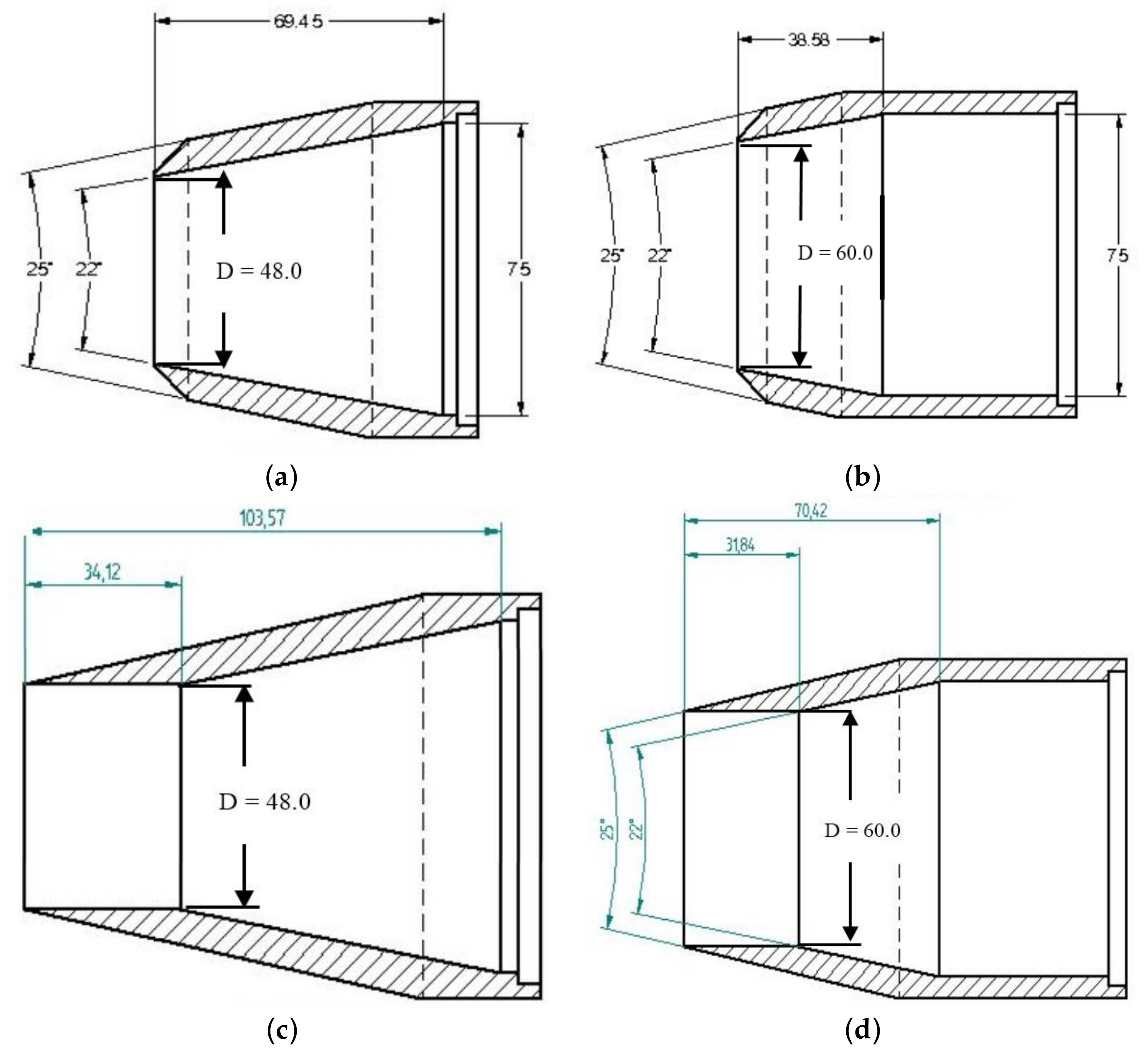
The nozzles used below comprised simple conical convergent designs, based broadly on the internal geometry of the BAE SYSTEMS Hawk jet trainer with an internal contraction half angle of 11°. Two nozzle exit sizes (D = 48 mm and 60 mm) were manufactured, labelled LU48 and LU60, see Figure 2a,b. Both nozzles had a short inlet section (OD = 86 mm, ID = 75 mm) followed by an axisymmetric convergent section; contraction lengths were 69.5 mm (LU48) and 38.6 mm (LU60). The nozzle lips featured a 45° chamfer (this improved optical access, allowing measurements to be made closer to nozzle exit, see below); final lip thickness was 1 mm. Two nozzle sizes allowed easier exploration of the influence of nozzle scale and Reynolds number. Two further nozzles were manufactured and included a short parallel extension at nozzle exit (different lengths for each nozzle size −34.1 mm in LU48P and 31.8 mm in LU60P, see Figure 2c,d). Nozzles with internal parallel wall exits have been observed to remove the vena contracta effect (R.A. Antonia and Q. Zhao [24]); this also allowed examination of the consequences of allowing the boundary layer to recover from the influence of the high favourable pressure gradient in the convergent section. Tests were performed at jet Reynolds numbers representative of engineering applications (ReJ > 106), with the nozzle operated at NPRs from 1.3 to 2.4, i.e., from low subsonic to supersonic (underexpanded) Mach numbers.
2.3. Instrumentation
2.3.1. Nozzle Inlet—Pneumatic Probe
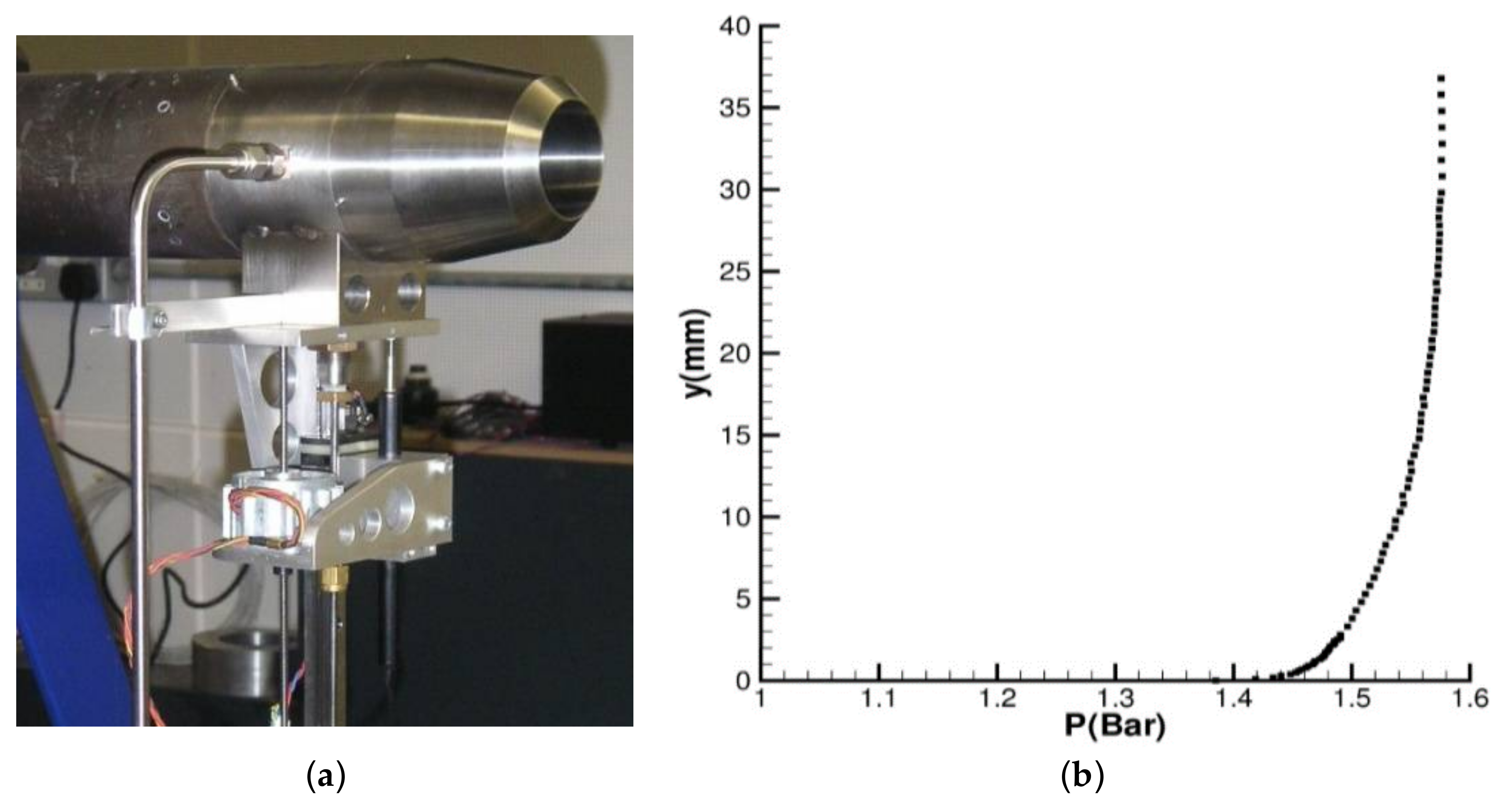
To confirm the turbulent nature of the nozzle inlet boundary layer and provide a quantitative specification of this, a boundary layer Pitot probe with a flattened measuring tip was used (thickness 0.32 mm, sensing opening 0.11 mm). Access just upstream of the nozzle was via the insertion of a short instrumentation section (70 mm long) between the high-pressure air supply pipe and the nozzle itself (see Figure 3a). This had two access ports (in the middle of the instrumentation section) spaced 90° apart azimuthally. The side port (2 mm diameter) was used as for a wall static pressure tapping and the lower port (3.1 mm diameter) as access for a Pitot probe traverse. The probe was traversed by a stepper motor with a positional accuracy of 0.013 mm. A typical traverse contained 90 points across the boundary layer, with resolution in the near-wall region of 0.1 mm and 1.0 mm towards the layer edge. Preliminary measurements across the whole pipe diameter indicated excellent symmetry. Measured total pressure (P), total temperature (T), and wall static pressure (ps) allowed calculation of axial velocity (U) using standard 1 D gas dynamic analysis assuming constant total temperature (T = 285 K). Figure 3b presents a typical total pressure profile showing a boundary layer of ~20 mm thickness due to the significant length of the delivery pipeline.
2.3.2. Nozzle Exit—Pneumatic Probe
Pitot probe measurements were also made at nozzle exit. Figure 3b indicated that the inlet boundary layer was relatively thick (~50% of the pipe radius); acceleration within the nozzle means the exit boundary layer was substantially thinner (as much as an order of magnitude). Further, exit dynamic pressure in the central core flow was significantly greater than at inlet and the slender inlet probe was unable to withstand the high aerodynamic loads. To address these problems and still allow measurements to be taken across the whole nozzle exit radius, a dual head Pitot probe was designed (Figure 4a). The miniature flattened head probe was still used in the near wall region but a reinforced Pitot probe (OD = 1.65 mm) was used to survey the outer region. The dual head probe was mounted on an arm (Figure 4b) and traversed using the system adopted for Laser Doppler Anemometry (LDA) measurements (see below). Measurements were made as close as possible to the nozzle exit plane but displaced 0.05 mm downstream. A wall tapping was not used to provide the static pressure; instead, the traverse was simply extended below the nozzle wall and (for an unchoked nozzle) the probe was then able to sense the local static pressure. A typical traverse from the near wall region illustrating (i) how thin the high gradient near wall region had become (~1 mm); (ii) how the wall location was identified (by extrapolation); and (iii) how the static pressure was obtained is given in Figure 5a; for comparison, a full radius traverse is shown in Figure 5b.
Because the technique described above involved measurements just outside the nozzle, it required consideration as to what extent the data was representative of the boundary layer exactly at nozzle exit. This question was addressed in S.C. Morris and J.C. Foss [25] by a study of a flat plate 2D equilibrium turbulent boundary layer (momentum thickness (θ) Reynolds number Reθ = 4650) flowing over a sharp straight trailing edge of the plate. The data indicated that profiles of statistical quantities in the free shear layer region were identical to the original boundary layer profile except for a very small region close to the wall y/θ0 < 2 (y is measured from the nozzle wall and θ0 is the momentum thickness at the trailing edge) for a distance of x/θ0 = 30 downstream of the plate edge. Analysis of pneumatic probe measurements (for both nozzle sizes) at the location 0.05 mm downstream of the nozzle trailing edge, the site chosen here for nozzle exit measurements, showed that the boundary layer momentum thickness θ0 varied between 0.025 mm and 0.035 mm over the NPR conditions explored (see Section 3.2 below). This implied that the measurement station was at x/θ0 = 1.5–2.0 downstream of the nozzle trailing edge, which is well within the 30θ0 distance shown in S.C. Morris and J.C. Foss [25] as the region where the profile outside the nozzle remained a good representation of the nozzle exit boundary layer. The chosen measurement location was thus considered acceptable.
2.3.3. Nozzle Exit and Jet Plume Region—LDA
To provide an alternative measurement of the nozzle exit velocity profile (particularly for higher subsonic Mach No. and supersonic conditions) and to establish a data set for mean velocity and turbulence statistics in the near-field jet plume region, a DANTEC fibre-optic two-component LDA system was employed. This comprised a 5 W Argon Ion laser, beam splitter, and manipulator; beam expanders to reduce the measuring volume size; a Bragg cell for frequency shifting (40 MHz); and a high-speed flow burst spectrum analyser (maximum measurable frequency of 180 MHz, which corresponds to a maximum measurable velocity of around 800 m/s). Measurements were taken in backscatter mode. The LDA optical parameters are provided in Table 1.
Liquid droplets with an average size 0.25 µm and density 920 kg/m3 were used for seeding and introduced ~2.0 m upstream of the nozzle to allow complete mixing across the pipe. For the underexpanded flow it was not possible to use liquid droplets. This was a result of the condensation of the moisture contained in the ambient-entrained air when it entered the higher speed jet regions which had low static temperature due to the high velocity, causing low signal to noise ratio. A solid particle seeder was substituted using aluminium oxide powder comprising 0.3 µm particles.
The validated data rate was typically 4 kHz with data taken (in transit time mode) for 5 s; 20 k readings were thus used to evaluate time-averaged statistics. The LDA system was traversed horizontally using a 3-axis DANTEC lightweight traversing table with a resolution of 6.25 μm in all axes. The LDA measuring volume was again located just downstream of nozzle exit, its distance now determined by the need for an unobstructed beam path across the whole boundary layer. The final location chosen was 0.375 mm downstream, i.e., at x/θ0 = 15, still within the region where data can be considered to represent nozzle exit.
2.3.4. Jet Plume Region—Schlieren Visualisation
The Schlieren method represents a useful technique to visualise shock wave characteristics in supersonic flow. The system used for the present study was a Z-type design and consisted of a Halogen lamp light source, two concave mirrors of 10 inch (254 mm) diameter, two planar round mirrors of 12 inch (305 mm) diameter, a knife-edge unit, and a Sony XCD-SX910CR digital camera. Instead of a standard unit, an orange-blue-green (rainbow filter) slide was used as a (horizontally-orientated) ‘knife-edge’. Orange colour on an image indicates a region of expansion, blue indicates a compression region, and green (corresponding to undeflected light) makes up a neutral background. Schlieren pictures were of an axial radial plane through the centreline of the jet plume and covered a distance of ~3D downstream of nozzle exit.
2.3.5. Data Processing/Derived Quantities
Velocity profiles in the boundary layer were extracted from measurements of Pitot pressure (P), total temperature (T), and static pressure (ps) using standard 1D gas dynamic relations. Thus, the local Mach number (M), static temperature (t), static density (ρ), and mean axial velocity (U) were determined from:
where R and γ are the gas constant and the ratio of specific heats for air (assumed as 1.4).
The boundary layers studied here covered a range of free stream Mach numbers up to high subsonic/supersonic. Accordingly, there will be considerable local variations in fluid density across the boundary layer. The consequence of this for the estimation of the integral properties of the boundary layer (displacement thickness (δ*) and momentum thickness (θ)) was studied in K.G. Winter and L. Gaudet [26] and L. Gaudet [27] for turbulent boundary layers with freestream Mach numbers 0.2 to 2.8. To calculate the compressible boundary layer integral profile quantities, these studies recommended the use of the ‘kinematic’ form (given the subscript ‘i’, where density variations are ignored) because this resulted in δ* and θ values independent of Mach number. Accordingly, this practice was adopted here. At nozzle inlet, the boundary layer overall thickness (δ) had been defined as the distance to the location where the velocity reached 99% of the centreline velocity. At nozzle exit, it was more convenient to locate the edge where the radial gradient of mean velocity was less than 1% of its maximum value (turbulence data showed this was in excellent agreement with the point where the turbulence stress decreased to its free stream value).
Kinematic forms of boundary layer properties (displacement and momentum thickness, shape factor, momentum thickness Reynolds number, wall friction velocity (-non-dimensional wall shear stress ), and skin friction coefficient ()) were obtained from the following (Rw is nozzle wall radius, y is orthogonal to the nozzle wall, and fluid properties are evaluated at the outer edge of the layer):
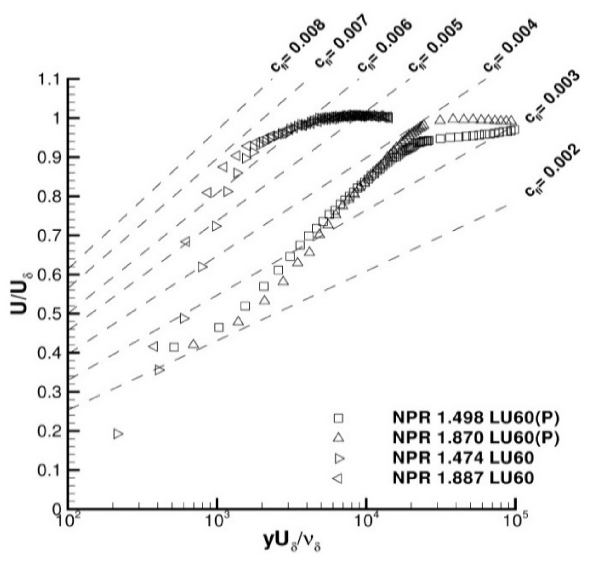
At nozzle inlet, the Clauser method [28] was used to calculate the skin friction coefficient. By multiplying both sides of the standard log-law formula by , the following expression results:
Equations (6) is used to generate a family of straight lines on a U/Uδ vs. ln (ρδUδy/μδ) chart for varying values of Cfi; experimental data when plotted on this chart identify the appropriate value of Cfi.
2.3.6. Measurement Errors
In all tests, gathering data for a single radial profile could be achieved within 5–6 min. The supply pressure control system was such that variations in NPR were typically less than ±1% during this time. For pneumatic probe measurements, the main source of experimental error was probe misalignment with the local flow direction (for probe data at Mach numbers avoiding local shock wave formation). The probe tip shape was chosen to reduce probe sensitivity to flow misalignment and a square-ended tip was selected, as recommended in E. Ower and R.C. Pankhurst [29], to provide less than 1% error in measured dynamic pressure for incidence less than 11° (the maximum encountered in the current study). This performance was confirmed for both probe types used here by testing in a separate low speed calibration facility. For LDA data, the statistical error was estimated assuming a 99% confidence level and a normal (Gaussian) probability distribution for velocity. For a validated sample size of 1000, this resulted in a measured mean velocity within ±0.05% of the true mean in the outer region of the boundary layer where the turbulence level is low (<2%). In the near wall region, where data rates were lower and turbulence levels higher (~20%), uncertainty increased to ±6% Applying the same analysis to the measured turbulence stresses, these are expected to lie within ±5% of the true value. The other source of error is that caused by LDA seed velocity bias. Using the approach of D.K. McLaughlin and W.G. Tiedermann [30], this was estimated as less than 5%, assuming a maximum turbulence intensity of 20%.
3. Results
3.1. Nozzle Inlet
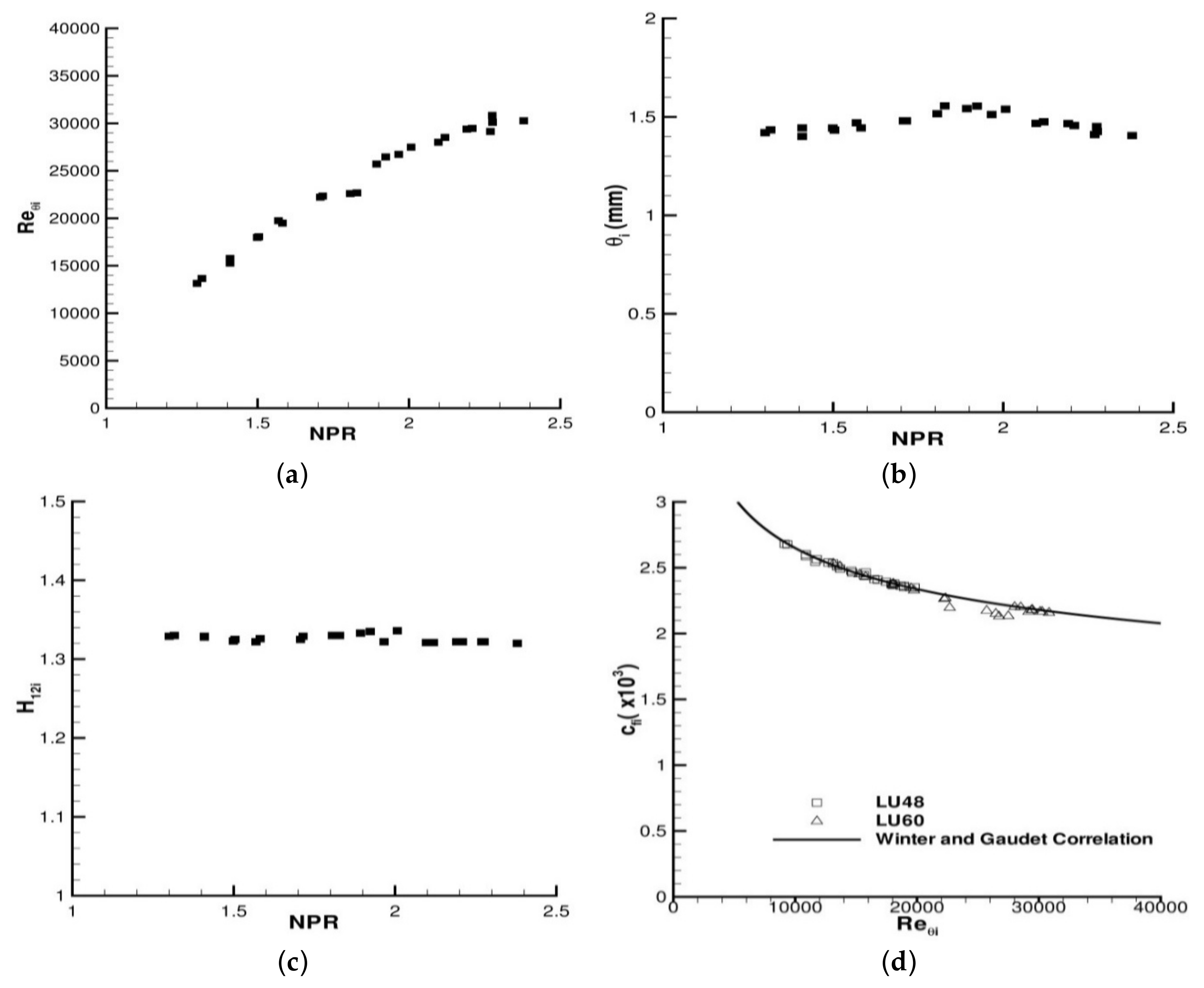
To avoid uncertainty over the state of the boundary layer at nozzle inlet (as occurred in previous studies, for example, W.C. Hill et al. [13,14] and J. Lepicovsky et al. [15]), and to provide specific inlet conditions for CFD prediction of the combined nozzle/plume flow, pneumatic probe measurements captured the boundary layer characteristics over the full range of NPRs tested (1.3–2.4) and both nozzle sizes (Note—it was not expected that the addition of the exit extension would influence inlet profiles so data was collected for the ‘clean’ nozzles only). Figure 6 shows the variation of Reθi, H12i, θi, and Cfi for the LU60 nozzle with increasing NPR (LU48 differences noted in the text below). Reθi showed a monotonic increase with NPR (by around a factor of three) with all values indicating a fully turbulent boundary layer (the trend for the LU48 nozzle was similar, although only increasing by a factor of ~2 (9000 to 19,000)). θi itself increased only slightly from 1.42 mm at NPR = 1.3, peaking at 1.5 mm at choking, and decreasing marginally thereafter (for LU48 the value stayed close to 1.45 mm for all NPRs). Centreline velocity and Mach number did not increase significantly with NPR in the smaller nozzle (0.23 < M < 0.28 for NPR = 1.3−2.4), whereas a larger change occurred in the LU60 nozzle (0.32 < M < 0.47). These numbers imply that, for the smaller nozzle, the increase in Reθi was primarily due to increase in core flow density, whereas for the larger nozzle, it was a result of increases in both free stream velocity and density. The overall thickness (δ) of the boundary layer varied only slightly from 21.8 mm (58% Rw) at NPR =1.3 to 19.4 mm (52% Rw) at NPR~2.4 (LU48 nozzle). The shape factor (H12i) values in Figure 6c support the conclusion that the boundary layer was fully turbulent (1.33 ± 0.01 for both nozzles). Finally, Figure 6d indicates that the skin friction coefficient data determined by the Clauser method (illustrated below in Section 3.2 shows excellent agreement for both nozzles with Equations (7), which represents the flat plate correlation deduced in [26]:
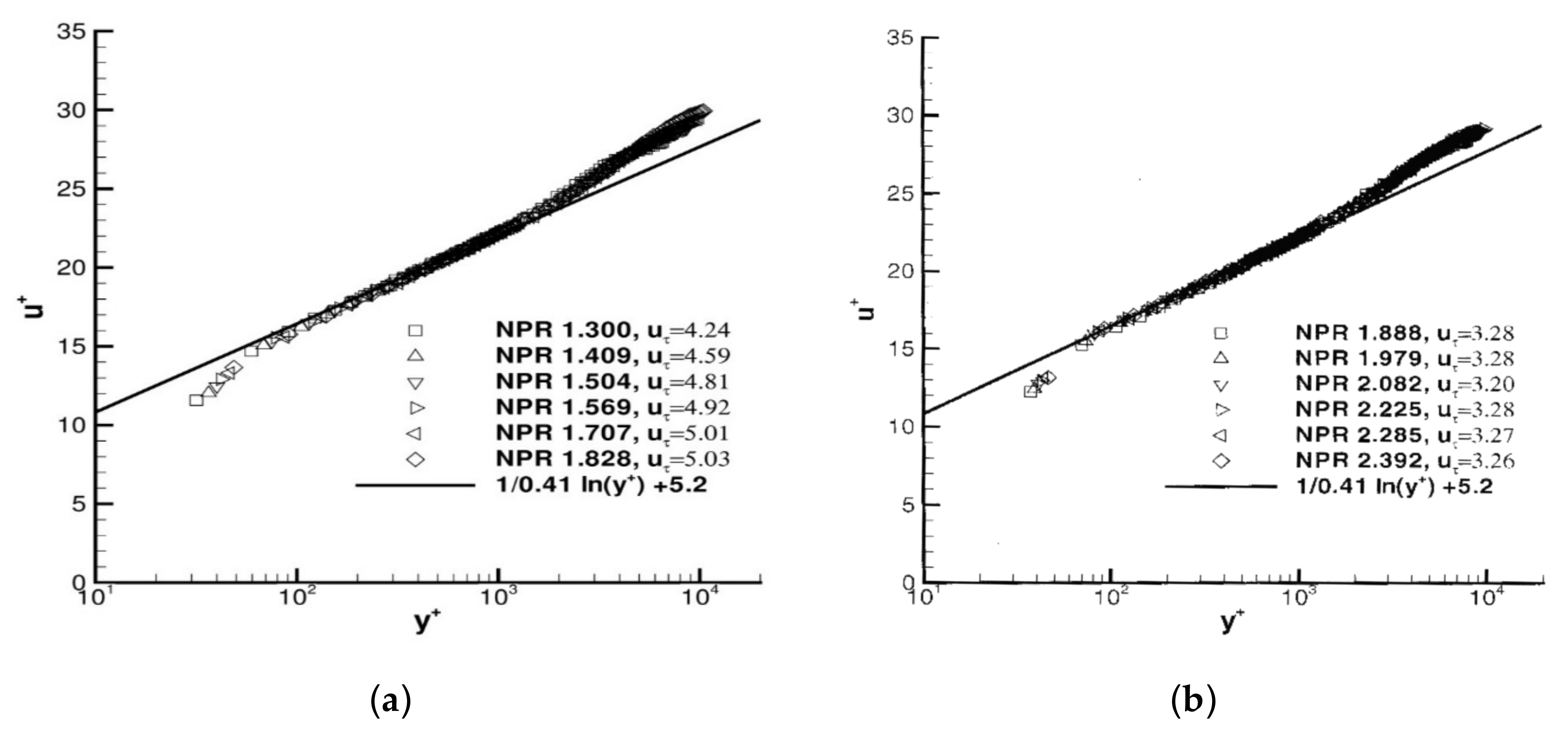
The wall friction velocity deduced from the Clauser plots was then used to convert the measured inlet velocity profiles to log-law format. Figure 7 presents data for a range of subsonic NPR for LU60 and for supersonic NPRs for LU48. All profiles show a large region following the standard log-law, extending from y+ ~150 to y+ ~1500 and a clearly defined wake region. Figure 6 and Figure 7 demonstrate that, for all NPRs, the inlet boundary layer corresponds closely to an equilibrium fully turbulent layer.
3.2. Nozzle Exit—‘Clean’ Nozzles LU48 and LU60
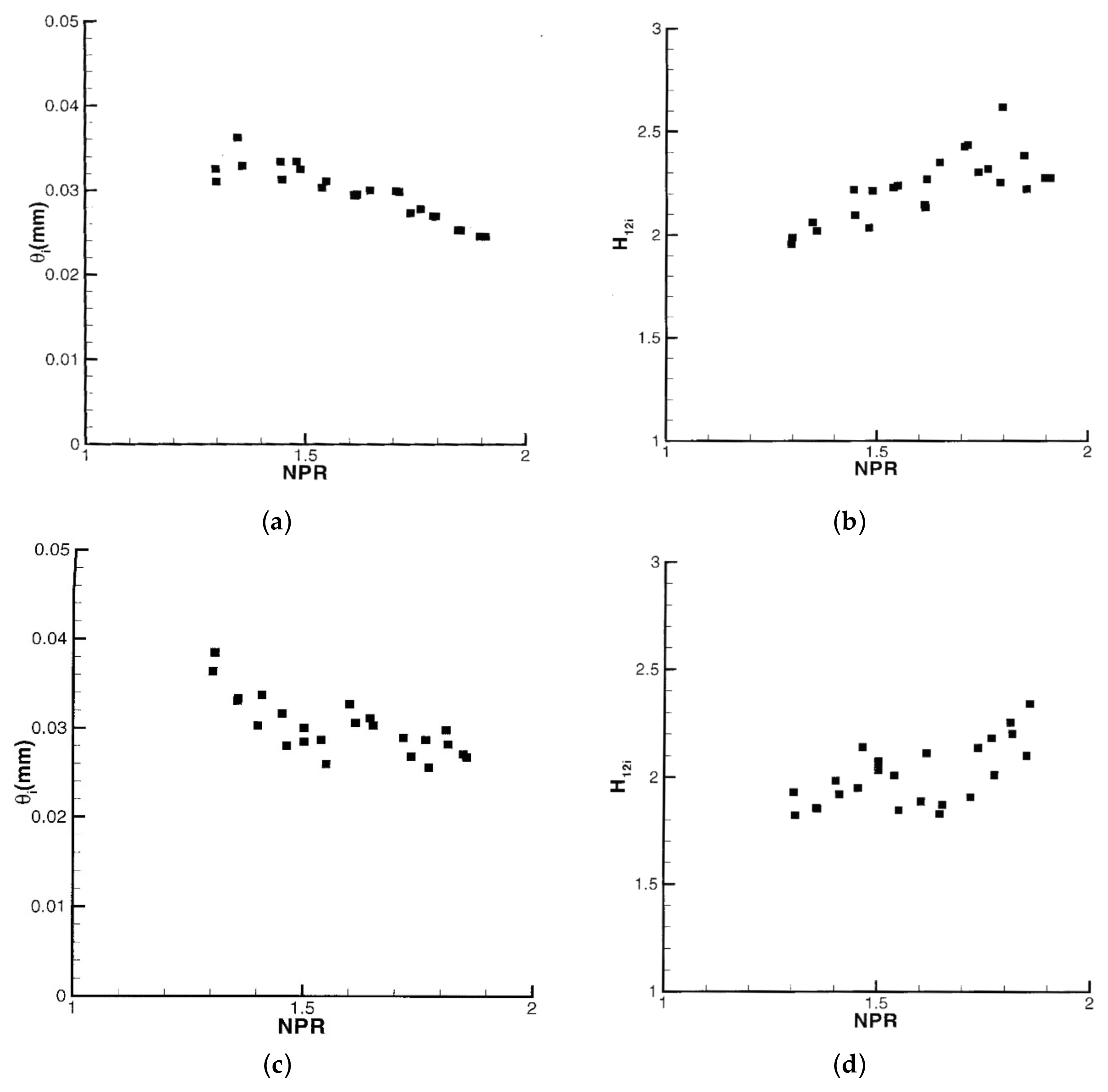
Pneumatic probe data were also obtained at nozzle exit; however, this was mainly carried out for unchoked NPRs since the presence of supersonic flow would introduce probe-induced shock waves and losses, which invalidate the assumption used in Equation (2). Therefore, LDA measurements were also made at nozzle exit for both subsonic (as a check) and higher NPRs. Probe-measured momentum thickness and shape factor data are presented in Figure 8 for both nozzles to compare against the inlet data in Figure 6. Two points are immediately apparent: firstly, as at the inlet, data at exit for both nozzle sizes reveal similar trends; secondly, the values and variation of θi and H12i with NPR are dramatically different to those seen at the inlet plane. For the LU48 nozzle, the value of θi is much reduced from an inlet value of θi = 1.42 mm, decreased at NPR =1.3 by a factor of ~40 to just 0.034 mm at exit. Further, whilst θi was effectively independent of NPR at inlet, it decreased significantly with NPR at exit, with the inlet to exit reduction factor increasing to ~60 at NPR = 1.89. The larger nozzle shows the same trends.
This dramatic thinning of the boundary layer-overall exit thickness δ for LU48 decreased to 0.5 mm (NPR = 1.3) and 0.375 mm (NPR = 1.89) can only be the result of the strong internal nozzle favourable pressure gradient. The corresponding values of Reθi (not shown) are 480–720 (LU48) and 550–750 (LU60), huge reductions on the ranges observed at inlet (9000–17,000 (LU48) and 13,000–30,000 (LU60)) in spite of the large increase in free stream velocity due to flow acceleration. The exit values of Reθi are in the range referred to as transitional or ‘laminarescent’ in H.H. Fernholz and P.J. Finley [31], i.e., boundary layers which contain turbulent fluctuations but also possess some laminar-like characteristics. This is borne out by the values of the shape factor H12i seen in Figure 8b,d; the inlet fully turbulent value of ~1.33 has been changed to a range from ~2.0 (NPR = 1.3) to ~2.3 (NPR = 1.89), implying a large shift in profile shape towards a laminar shape (a Blasius boundary layer has H12 = 2.59).
Figure 9 further illustrates the changing profile shape by comparing exit and inlet mean velocity profiles for the LU60 nozzle (results for LU48 are identical). Profiles were plotted using wall normal distance scaled using inlet (or exit) displacement thickness δi* to non-dimensionalise the y co-ordinate rather than overall boundary layer thickness δ as would be more usual. This was done as estimation of δ was found to be subject to significantly larger measurement errors than estimation of δi* for the very thin exit boundary layer. Only one inlet profile is shown since Figure 5 and Figure 6 have confirmed the inlet profile displays no change with NPR. No observable change in exit profile shape is again seen with NPR in this plot; however, as noted above, the shape factor does increase slightly with NPR. The near-wall gradient is much shallower than at nozzle inlet, implying that the exit profile shape is much more laminar-like than the fully turbulent inlet profile. This implies that the strength of acceleration within the nozzle has created a transitional, partly re-laminarised exit boundary layer. Clauser plots of inlet and exit data are provided in Figure 10. Inlet profiles at two NPRs display clearly defined logarithmic regions (enabling Cfi to be identified as described above). In contrast, for the exit profiles no obvious logarithmic region exists. It should be noted that, although the nozzle exit wall shear stress value cannot be clearly established, Figure 10 implies that the level of Cfi is greater at exit than at inlet. This appears to contradict the information shown in Figure 9, where the near wall velocity gradient is greater at inlet than at exit. This anomaly is a result of the use of very different values of δi* for the inlet and exit profiles in Figure 9 (the inlet value is~20 times greater at inlet than at exit). However, Figure 8, Figure 9 and Figure 10 unequivocally demonstrate that the exit profile is strongly influenced by the acceleration experienced within the nozzle, and that the resulting profile shape is far removed from that corresponding to an equilibrium turbulent boundary layer.
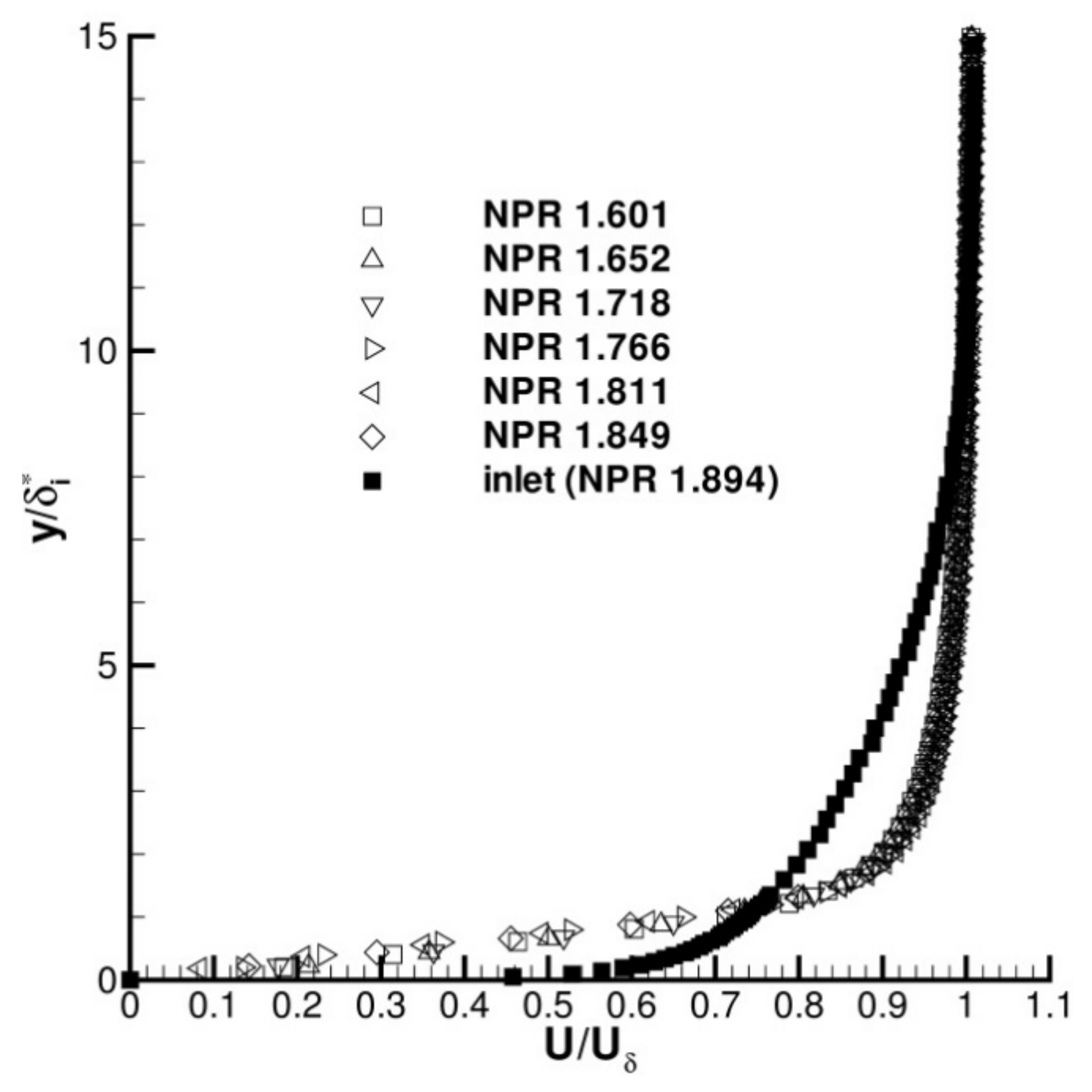
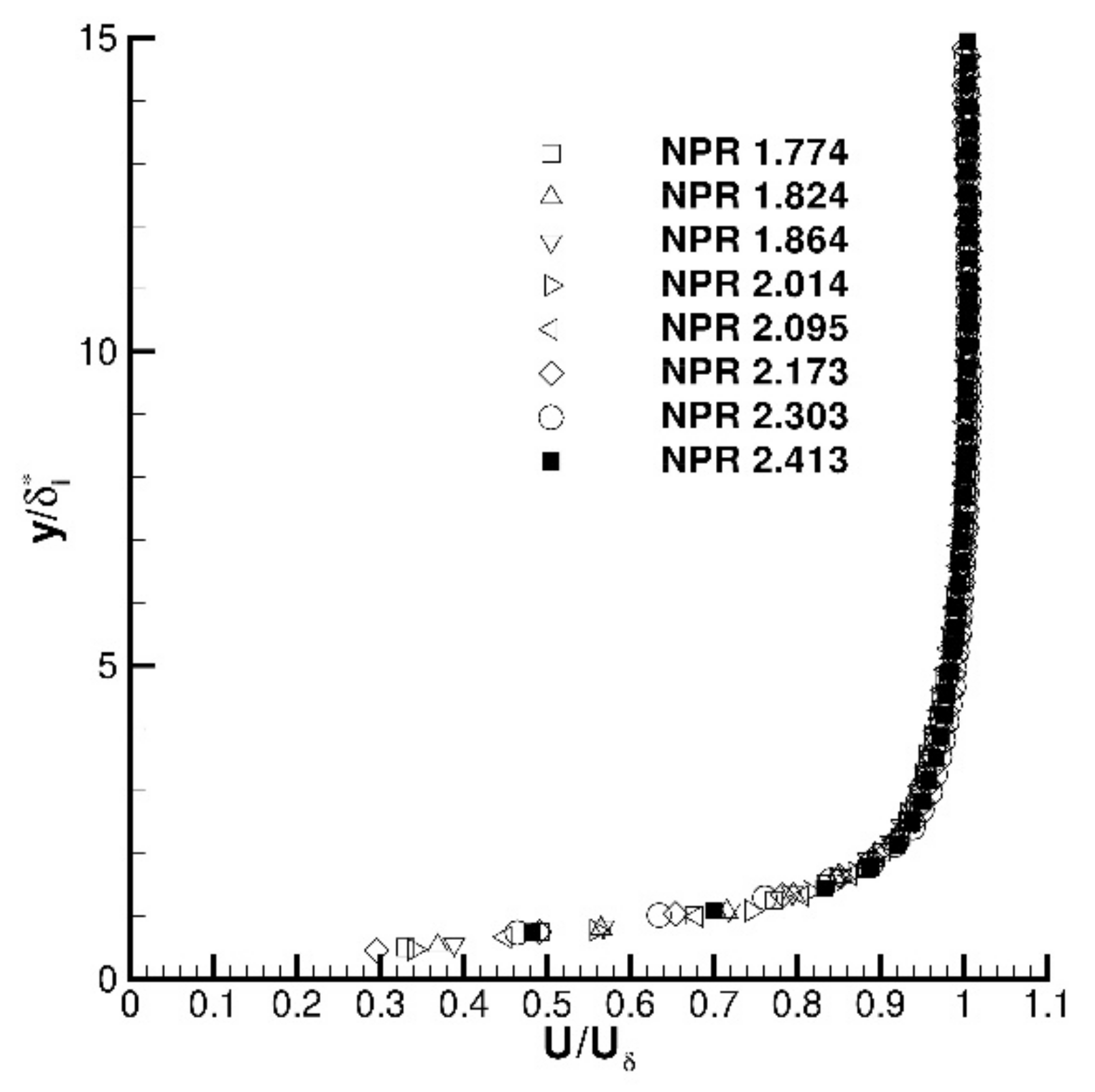
Figure 10 also contains a comparison between probe-measured and LDA-measured exit velocity profiles for two NPRs. Agreement on profile shape between the two methods of measurement is good at the lower NPR (~1.3), but even for NPR = 1.8, flow acceleration over the probe has clearly already introduced local shock loss effects and the LDA and probe-measured profiles deviate from each other. The LDA data do not suffer from any blockage and associated acceleration effects and also show good agreement between the two NPR results. This issue is further illustrated by the comparison of shape factor data shown in Figure 11. Probe and LDA results agree well until around NPR ~1.7 but then diverge. The LDA data indicate that H12i continues to grow with NPR but at a slower rate than is implied by the probe data for NPR > 1.7. There is some scatter, but the LDA data show a consistent tendency for the profile to shift continually towards a more laminar state as NPR increases beyond the critical NPR and well into the underexpanded regime. It must be remembered that, as the jet plume begins to assume an underexpanded state, a Prandtl–Meyer expansion fan will form and emanate from the nozzle lip. As measurements were made a small distance downstream, it is possible that the effect of passing through the expansion fan has also contributed to the profile shape. LDA measure non-dimensional mean velocity profiles for high subsonic and underexpanded NPRs are shown in Figure 12. The measurements collapse well for all NPRs, indicating little noticeable effect of the expansion fan effects mentioned above.
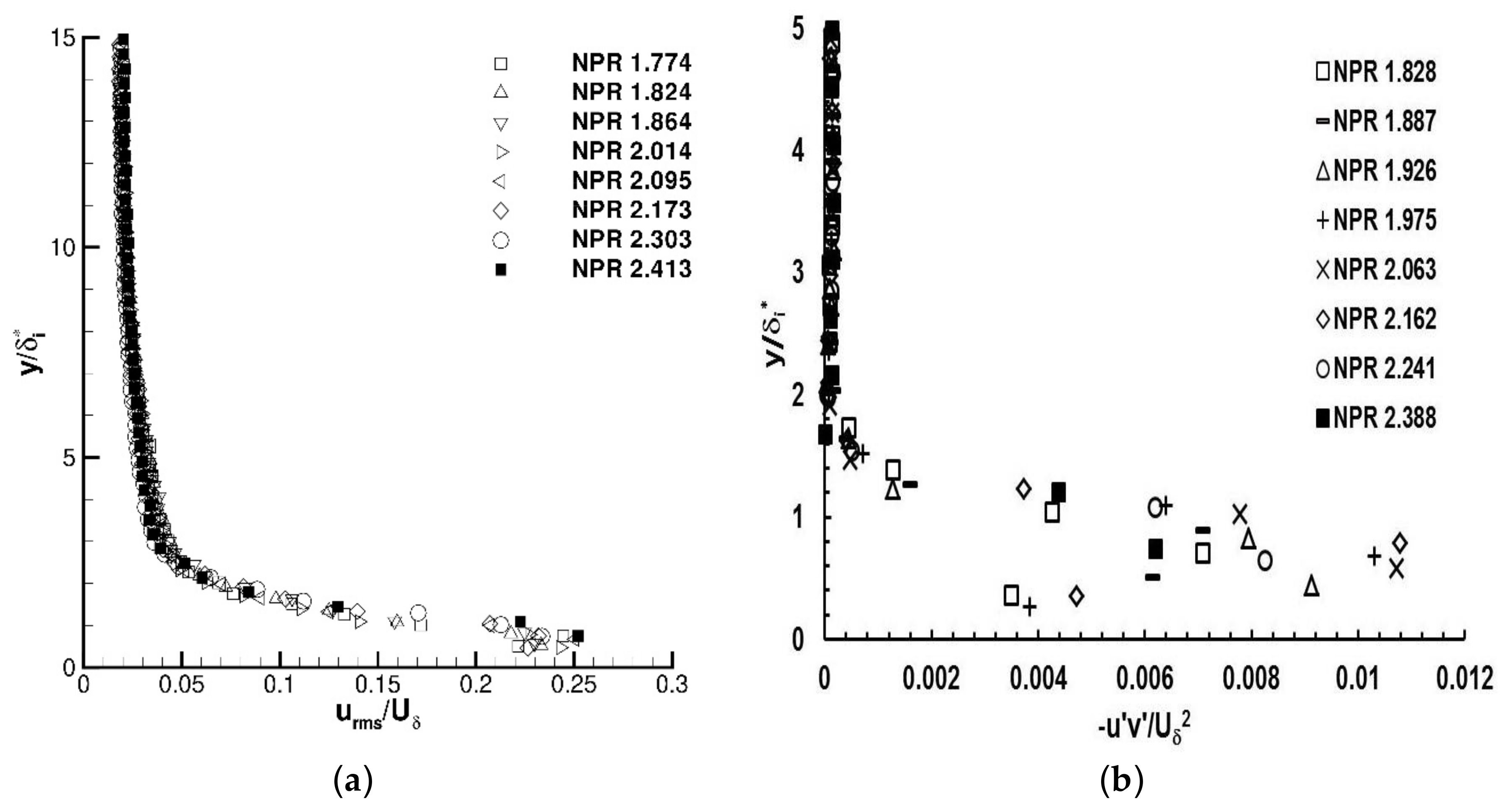
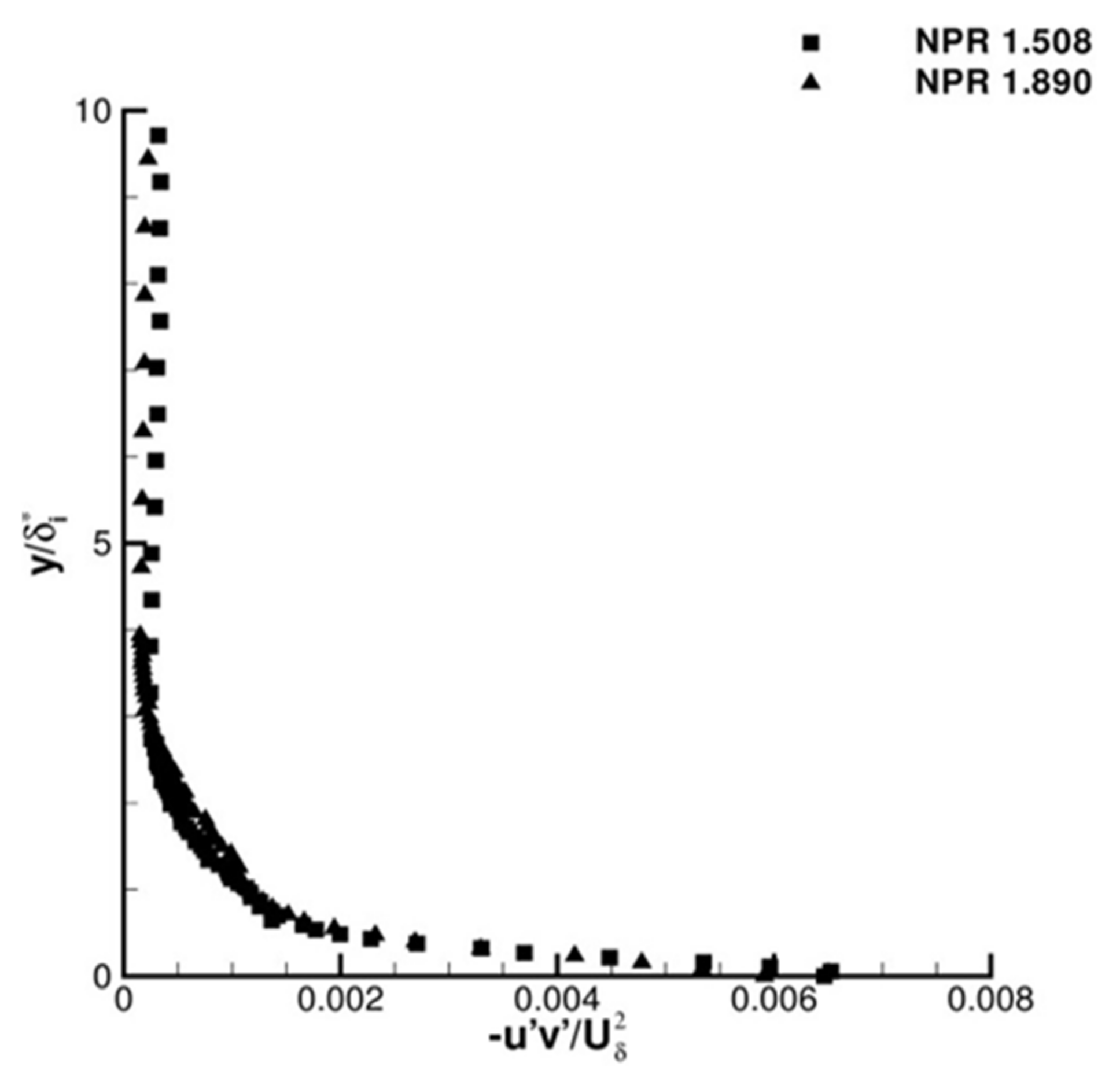
Figure 13 examines LDA data for turbulence Reynolds stresses in the nozzle exit boundary layer. Here, emphasis is given to data at high subsonic Mach No. and at underexpanded NPRs. Figure 13a show the axial rms profile and Figure 13b presents the Reynolds shear stress. As expected for such thin boundary layers, the peak values are located close to the wall. The peak values of show a slight increase with NPR, which was also noted in D. Warnack and H.H. Fernholz [19]. As the strength of the favourable pressure gradient increases (with NPR) and the layer thickness decreases, the near wall velocity gradient (and hence ) increases and the near wall turbulence level increases in proportion. For the non-dimensional shear stress (−), the peak value first increases from ~0.007 at NPR = 1.83 to a maximum of ~0.011 at NPR = 2.1, then decreases rapidly to ~−0.006 at the highest NPR = 2.39. The decreasing behavior is likely caused by the growing strength of the expansion fan region counteracting the effects of the internal nozzle acceleration.
3.3. Nozzle Exit—The Influence of a Parallel Walled Nozzle Exit Extension—Nozzles LU48P and LU60P
D. Warnack and H.H. Fernholz [19] showed that a laminarescent boundary layer recovers rapidly from the effects of a favourable pressure gradient, once removed. This is examined by comparing nozzle exit data for LU60 and LU60P geometries (smaller nozzle data were similar). Table 2 shows the effect of a parallel extension on exit boundary layer integral parameters at two subsonic NPRs. The extension has significantly altered the thickness and shape of the exit boundary layer. Both NPRs indicate similar behaviour: from the same fully turbulent boundary layer at inlet, the clean nozzle shows an extremely thin exit boundary layer with a laminarescent shape factor and very low momentum thickness Reynolds number. With the short parallel extension, the exit boundary layer has a momentum thickness a factor ~14 times larger than for a convergence only nozzle, with Reθi values ~16 times larger, and a turbulent rather than a laminar-like shape factor (1.22 (LU60P) compared to 2.0 (LU60)). The rapid recovery observed in D. Warnack and H.H. Fernholz [19] is replicated in the present tests with the addition of a relatively short (~0.5D) parallel extension.
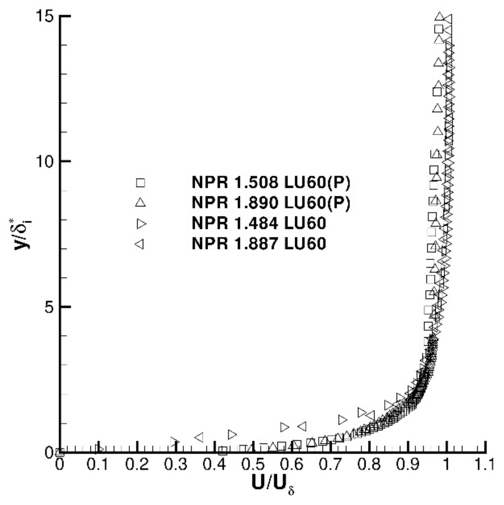
Further illustration of these changes may be seen in the measured exit velocity profiles presented in Figure 14 and Figure 15. Figure 14 shows that the exit flow with extension displays a fuller, more turbulent shape with a steeper near-wall gradient. The extent of recovery to fully turbulent flow is seen better in Figure 15, which presents the same exit profiles in semi-logarithmic Clauser plot form. The profiles with extension have not fully recovered to an equilibrium turbulent state and do not possess any clearly defined equilibrium log-law region; however, they are much closer to this than the profiles from the convergence only nozzle. In the LU60P data, a short region may be identified (approximately 103 < y+ < 2 × 10³) which does not follow the lines of constant Cfi deduced from an equilibrium log-law but has a steeper gradient, which is described in A.D. Young [32] as evidence of adverse pressure gradient effects. The most likely origin is the flow turning associated with the internal corner between the convergent nozzle wall and the parallel extension wall, see Figure 2c,d.
Finally, turning to LDA-measured turbulence at nozzle exit, Figure 16 and Figure 17 show profiles for non-dimensional axial rms and Reynolds shear stress. Comparison of axial rms data for nozzles with convergence only and with added extension indicates that allowing boundary layer recovery leads to a decrease in peak value, likely caused by turbulence adjusting to the decreased level of wall shear (see Clauser plots in Figure 15). The peak value location is also shifted very close to the wall. The shear stress profile (Figure 17) shows a similar peak value of ~0.007 (compare with convergence only data for NPR = 1.89 in Figure 13b) but a significant near wall shift is observed.
3.4. Jet Plume Region
Similar trends in the behavior of the nozzle exit boundary layer were observed with both nozzle sizes. Accordingly, the test conditions for the jet plume study were restricted to the smaller nozzle (LU48/LU48P) because this required smaller mass flow rates and allowed longer test durations. Three NPRs at high subsonic and underexpanded conditions—NPR = 1.5, 1.88, and 2.4—were selected for study. Figure 18 displays LDA-measured axial profiles of mean and fluctuating rms axial velocity along the nozzle axis (r/D = 0.0) and the nozzle lipline (r/D = 0.5) for the almost choked condition (NPR = 1.88). The first measurement location was 4 mm from nozzle exit (x/D = 0.083) and measurements extended over the first 10 nozzle diameters. In terms of centreline velocity development, the addition of a short parallel extension produced no discernable effect on either the initial decay rate of the centerline velocity or the potential core length, xpc/D = 6.8, i.e., the location when U/Upc = 0.99 (where Upc is the velocity within the potential core). Figure 18a shows data for NPR =1.88, but it was noted that xpc/D = 6.2 was observed for NPR = 1.5, showing the start of the compressibility-induced slower shear layer spread as jet Mach No. increases. The variation of centreline axial turbulence rms is shown in Figure 18b; no difference between LU48 and LU48P data is seen. Notably, the behaviour for 2.0 < x/D < 6.5 was within the constant velocity potential core region and would it not be expected that any shear generation of turbulence would occur. However, urms increased significantly in this region but at a rate less than for x/D > 6.8, when the annular shear layer reached the centreline and radial shear-driven turbulence production had begun. Therefore, this was not genuine turbulence but rather unsteady inviscid flow, which is sensed by the LDA system and contributes to the urms measured. urms remained constant at the turbulence level corresponding to the nozzle core flow up to x/D = 2.0, but then began to increase. Similar behaviour was noted in the data presented in O. Power et al. [33], caused by local irrotational unsteadiness induced by the downstream passage of large turbulent eddies in the initial region of the shear layer. Unlike the centreline profile, lipline axial velocity profiles show significant variation between LU48 and LU48P. The LU48P data (Figure 18c) initially showed a small decrease, followed by an increase in the first dimeter of axial development, and then a gradual decrease as expected at an entraining boundary. The convergence only nozzle indicated a much lower velocity at nozzle exit which subsequently rapidly increased, consistent with the more laminar-like boundary layer and the vena contract effect. For axial velocity, differences between LU48 and LU48P are still visible at x/D = 10, but on lipline turbulence differences disappear at around x/D = 4.0, with the LU48P data noticeably above the LU48 data only in the first diameter.
Similar data for development along jet centreline and nozzle lipline for an underexpanded jet plume (NPR = 2.4) are presented in Figure 19. Axial velocity variation is presented in Figure 18a (and in Figure 18b for an enlarged view of the first five diameters). Note that the reference velocity used here for non-dimensionalisation is the ideal fully expanded velocity (for NPR = 2.4, Tamb = 285 K, Uexpanded = 354 m/s). The presence of shock cell oscillations of decreasing amplitude up to x/D~6 was clearly visible, with 10 cells detected. Velocity increased as the flow was accelerated through expansion fans, followed by a sharp decrease as it was decelerated by oblique shock waves. Unlike the near-field behaviour observed for the subsonic plume, there were significant differences throughout the potential core region between the two nozzle shapes for the improperly expanded jet. The nozzle exit velocity for LU48 was lower than for LU48P: 0.76Uexpanded versus 0.88Uexpanded. The greater degree of external expansion for the convergence only nozzle was caused by the vena contracta effect. The first shock cell length was also smaller after the addition of the exit parallel extension: 0.74DJ versus 0.84DJ although subsequent shock cell lengths were essentially similar. Potential core length was ~5% longer for the LU48 nozzle (x/D = 6.0 versus 5.7 for LU48P), causing a downstream shift of the onset of centreline velocity decay. The centreline turbulence results showed large fluctuations in magnitude within the potential core region at locations corresponding to the locations of the oblique shock waves. These were unlikely to have been caused by shock-induced turbulence (they do not occur in measurements of vrms (not shown)) but were artifacts introduced by the effects of LDA seed particle velocity lag as they passed through regions of high acceleration/deceleration. On the lipline, mean velocity differences were only apparent over the first two diameters; however, lipline turbulence was ~20% higher for the nozzle with added extension for the whole downstream distance measured.
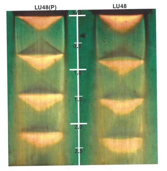
A useful overall picture of the immediate jet near-field (0 < x/D < 3) can be seen in the colour Schlieren image provided in Figure 20. The greater length of the first shock cell for LU48 is apparent, as is a different shape of the first flow expansion zone immediately after nozzle exit (particularly near the centreline) with a larger orange region whose boundary is also more convex than in the LU48P results. These are clear consequences of vena contracta effects. The presence of significant radially inward velocities indicates that the near centreline flow did not experience the same degree of expansion in the contraction only nozzle as in the nozzle with the extension. The centreline static pressure is thus higher in the contraction only nozzle. A greater degree of expansion outside the nozzle is required to achieve pressure equilibrium; the angle of the expansion fan increases and accordingly, the shock cell length is greater. The oblique shock wave’s structure, formed by the coalescence of the reflected Mach waves forming the expansion fan, also changes. These differences in expansion/compression region structure between the two nozzles decreases in subsequent shock cells but small differences are still visible up to the fifth cell.
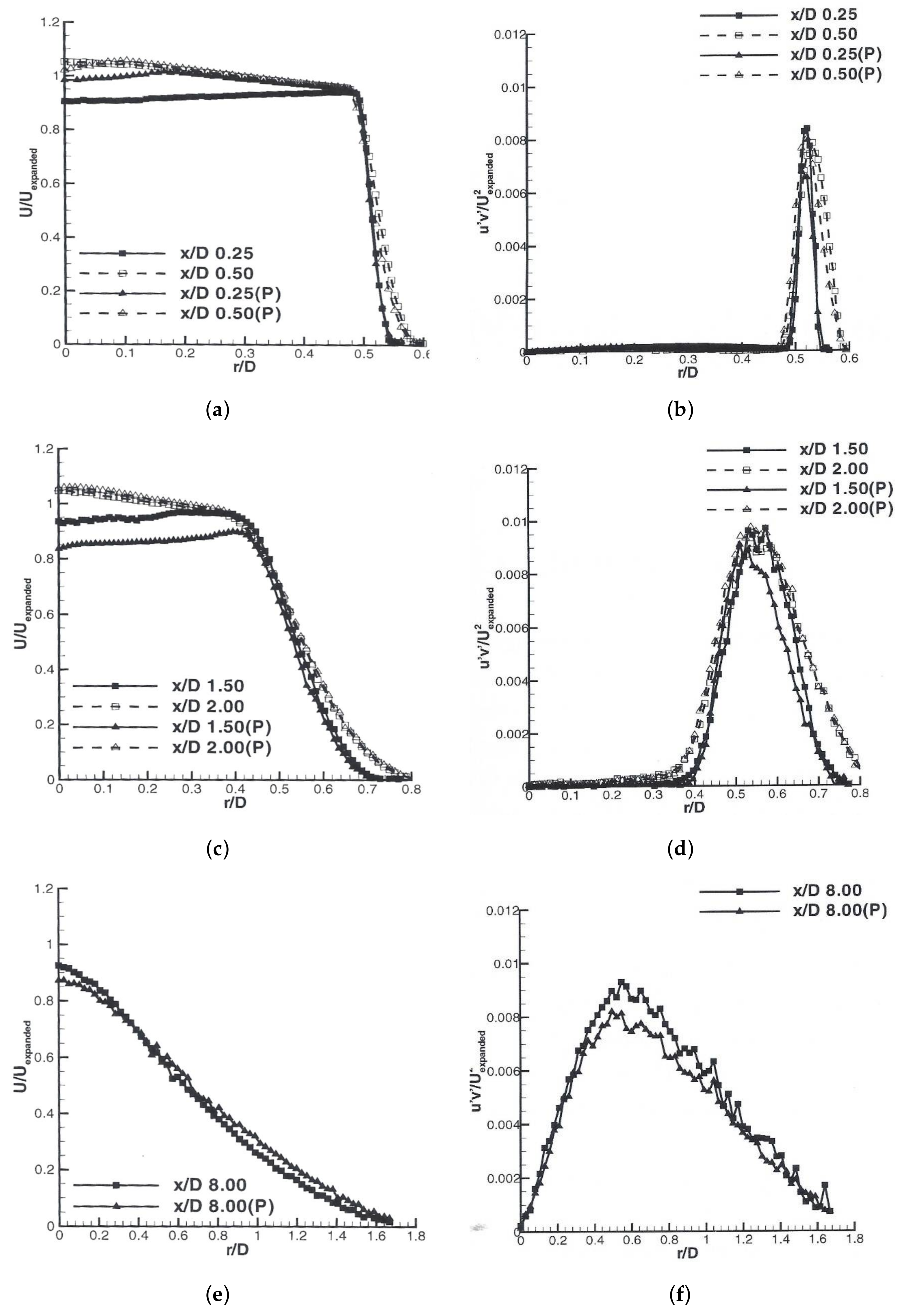
Finally, the effects of the vena contracta are also apparent in the radial profiles of mean velocity and turbulent Reynolds stress given in Figure 21. Large variations between the profiles for the two nozzle geometries can be seen within the supersonic region, depending on whether the measurement locations correspond to the position of an expansion or recompression region This is particularly the case at x/D = 0.25 and 2.0, but small differences can still be seen at x/D = 8.0. These differences appear predominantly in the inviscid flow region. The velocity distributions in the shear layer follow similar trends; however, at x/D = 8.0, the variations have accumulated to produce a slightly wider and more diffused jet for the nozzle geometry with small parallel extension. The turbulent shear stress data initially (x/D = 0.25, 0.5, Figure 21b) show little difference between the two nozzle shapes. Further downstream at x/D = 1.5, the convergence only nozzle seems to show a slightly higher peak value and a greater radially outward extent of the shear layer, but this has disappeared by x/D = 2.0 although at x/D =8.0 the larger peak shear stress of LU48 has returned despite the mean velocity profile showing less diffusion than LU48P.
4. Summary and Conclusions
Near-field flow development of high subsonic, supersonic, and improperly expanded jets is an important topic in aero-engine propulsion for jet noise and infrared signature reduction. Details of the flow within the propulsion nozzle determine the nozzle exit boundary layer characteristics (laminar or turbulent, thickness, turbulence levels) which are the initial conditions for the jet plume near-field. Whilst this subject has been addressed extensively, many of these studies have been at too low Reynolds or Mach Nos. and underexpanded jets have been so far ignored. This has motivated the work reported here, which has intentionally focused on nozzle geometries and operating conditions (principally Nozzle Pressure Ratio (NPR)) similar to those found in aero-engine propulsion applications. Particular attention has been placed on establishing a database of measurements for both nozzle inlet and exit conditions as well as on the jet plume to fill the gaps and avoid the uncertainties of previous studies.
Two nozzle geometries were chosen: a convergence only design and the same nozzle with a short parallel extension at nozzle exit. Two measurement techniques were used to provide a complete survey of relevant flow properties, enabling provision of a comprehensive CFD validation data set. Measurements at nozzle inlet demonstrated unequivocally that, for all NPRs tested, the nozzle inlet conditions corresponded to a fully turbulent equilibrium boundary layer (shape factor H12i = 1.33). In contrast, for the convergence only design, both pneumatic probe and LDA measurements at nozzle exit indicated clear evidence of re-laminarisation (shape factor H12i = 2.0–2.3). Exit profiles of axial velocity and turbulence quantities showed that the profile was ‘laminarescent’, i.e., still possessing turbulent fluctuations but displaying many laminar-like properties. The addition of a short parallel extension revealed a much thicker profile (~ factor of 10 increase) and a rapid return towards more turbulent profile characteristics (shape factor H12i = 1.22). The relationship between nozzle exit boundary layer characteristics and vena contracta effects was thus shown to be inextricably linked to nozzle geometry. For a convergent only geometry the internal nozzle acceleration created an exit profile shape which indicated partial relaminarisation and an extremely thin boundary layer; the presence of radially inward velocities at nozzle exit also caused significant vena contracta effects, e.g., continued centreline jet velocity increase outside the nozzle for ~1D. In contrast to this, the addition of a short parallel extension to the convergent only geometry allowed boundary layer recovery, so that the nozzle exit characteristics displayed an order of magnitude increase in boundary layer momentum thickness and a much more turbulent profile shape (shape factor ~1.2); radial velocities were also eliminated, so there was little indication of any vena contracta effects. Measurements in the jet plume near-field for the convergence only nozzle at an almost choked NPR showed vena contracta effects extended to 8D on the nozzle lipline. These were almost entirely absent with the addition of an exit parallel extension, with lipline turbulence also reduced in the first 2D compared to the convergence only case. Centreline, lipline and radial profile data and Schlieren imaging revealed marked vena contracta effects in the case of an under-expanded jet (NPR = 2.4). Shock cell length (in particular the first) was longer than for the convergence only nozzle, leading to a noticeable increase in potential core length.
In summary: (i) the measurements reported here have extended the available data into the underexpanded regime; (ii) the effect of a short parallel extension at nozzle exit has been shown to have a dramatic effect on both exit boundary layer characteristics and vena contracta effects; (iii) in addition, by providing nozzle inlet and exit profile data and details of the resulting jet plume near-field velocity and turbulence characteristics under representative operating conditions, the data presented here are believed to create an excellent validation test case for assessment of CFD predictive capability.
Acknowledgments
Financial support for this project was received from EPSRC (Grant Number GR/02300852) and from BAE SYSTEMS (Warton, Lancashire, UK).
Author Contributions
Parviz Behrouzi was responsible for the design and commissioning of the test facility; Miles T. Trumper designed the nozzle test cases, instrumentation, and performed the experiments; Miles T. Trumper and James J. McGuirk analysed the data; James J. McGuirk produced the written paper.
Conflicts of Interest
The authors declare no conflict of interest. The funding sponsors had no role in the design of the study, in the collection, analyses, or interpretation of data, in the writing of the manuscript, and in the decision to publish the results.
Nomenclature
| a | Speed of sound |
| B | Constant in log-law expression |
| CFD | Computational Fluid Dynamics |
| Skin friction coefficient | |
| D | Nozzle exit diameter |
| dx, dy, dz | LDA measurement volume size |
| Kinematic shape factor = | |
| IR | Infra-Red |
| Boundary layer integral parameters | |
| LDA | Laser Doppler Anemometry |
| L | LDA focal length |
| MC | Convective Mach number |
| MJ | Jet Mach number = UJ/aJ |
| NPR | Nozzle Pressure Ratio |
| Nf | Number of LDA fringes |
| P | Total pressure |
| ps | Static pressure |
| RANS | Reynolds Averaged Navier Stokes |
| ReJ | Jet Reynolds number |
| Reθi | Momentum thickness Reynolds number |
| Rw | Radius of pipe wall |
| s | LDA fringe spacing |
| t | Static temperature |
| T | Total temperature |
| U | Axial mean velocity |
| urms | Axial turbulent rms velocity |
| u+ | Non-dimensional log-law velocity |
| u′v′ | Reynolds shear stress |
| uτ | wall friction velocity = |
| xpc | Potential core length |
| y | Distance normal to wall |
| y+ | Non-dimensional log-law wall distance |
| Greek symbols | |
| Overall boundary layer thickness | |
| Kinematic displacement thickness | |
| κ | Von Karman constant |
| λG | LDA green beam wavelength |
| λB | LDA blue beam wavelength |
| ρ | Density |
| θ | LDA beam angle |
| θi | Kinematic momentum thickness |
| τw | Wall shear stress |
| μ | Absolute viscosity |
| υ | Kinematic viscosity |
| Subscripts | |
| J | Jet properties |
| δ | Boundary layer edge properties |
| amb | Ambient property |
| 1, 2 | Fast and slow moving streams |
References
- Papadopolous, G.; Pitts, W.M. Scaling the near-field centreline mixing behaviour of axisymmetric turbulent jets. AIAA J. 1998, 36, 1635–1642. [Google Scholar] [CrossRef]
- Bradshaw, P. The effect of initial condition on the development of a free shear layer. J. Fluid Mech. 1966, 26, 225–236. [Google Scholar] [CrossRef]
- Ricou, F.P.; Spalding, D.B. Measurements of entrainment by axisymmetrical turbulent jets. J. Fluid Mech. 1961, 11, 21–32. [Google Scholar] [CrossRef]
- Pitts, W.M. Reynolds number effects on the mixing behaviour of axisymmetric turbulent jets. Exp. Fluids 1991, 11, 135–141. [Google Scholar] [CrossRef]
- Xu, G.; Antonia, R.A. Effect of initial conditions on the temperature field of a turbulent round jet. Int. Commun. Heat Mass Transf. 2002, 29, 1057–1068. [Google Scholar] [CrossRef]
- Papamoschou, D.; Roshko, A. The compressible turbulent shear layer: An experimental study. J. Fluid Mech. 1988, 197, 453–477. [Google Scholar] [CrossRef]
- Barone, M.F.; Oberkampf, W.L.; Blottner, F.G. Validation case study: Prediction of compressible turbulent mixing layer growth rate. AIAA J. 2006, 44, 1488–1497. [Google Scholar] [CrossRef]
- Sarkar, S.; Lakshmanan, B. Application of a Reynolds stress turbulence model to the compressible shear layer. AIAA J. 1991, 29, 743–749. [Google Scholar] [CrossRef]
- Yoder, D.A.; DeBonis, J.; Georgiadis, N.J. Modelling of turbulent shear free flows. Comput. Fluids 2015, 117, 212–232. [Google Scholar] [CrossRef]
- Lau, J.C. Mach number and temperature effects on jets. AIAA J. 1980, 18, 609–610. [Google Scholar] [CrossRef]
- Lau, J.C. Effects of exit Mach number and temperature on mean flow and turbulence characteristics in round jets. J. Fluid Mech. 1981, 105, 193–218. [Google Scholar] [CrossRef]
- Feng, T.; McGuirk, J.J. Measurements in the annular shear layer of high subsonic and underexpanded round jets. Exp. Fluids 2016, 57, 7. [Google Scholar] [CrossRef] [Green Version]
- Hill, W.C.; Jenkins, R.C.; Gilbert, B.L. Effects of the Initial Boundary Layer State on Turbulent Jet Mixing; Technical Report AFAPL-TR_75–67; Grumman Aerospace Corp.: New York, NY, USA, 1975. [Google Scholar]
- Hill, W.G.; Jenkins, R.C.; Gilbert, B.L. Effects of the initial boundary layer state on turbulent jet mixing. AIAA J. 1976, 14, 1513–1514. [Google Scholar] [CrossRef]
- Lepicovsky, J.; Ahuja, K.K.; Brown, W.H.; Salikuddin, M.; Morris, P.J. Acoustically Excited Heated Jets; NASA Contractor Report 4129; NASA Lewis Research Centre: Hampton, VA, USA, 1988.
- Lepicovsky, J. The role of nozzle exit boundary layer velocity gradient in mixing entrainment of free shear flows. In Proceedings of the 3rd ASCE/ASME Mechanics Conference, La Jolla, CA, USA, 9–12 July 1989. [Google Scholar]
- Narasimha, R.; Sreenivasan, K.R. Re-laminarisation in highly accelerated turbulent boundary layers. J. Fluid Mech. 1973, 61, 417–447. [Google Scholar] [CrossRef]
- Warnack, D.; Fernholz, H.H. The effects of a favourable pressure gradient and of the Reynolds number on an incompressible axisymmetric turbulent boundary layer—1: The turbulent boundary layer. J. Fluid Mech. 1998, 359, 329–356. [Google Scholar] [CrossRef]
- Warnack, D.; Fernholz, H.H. The effects of a favourable pressure gradient and of the Reynolds number on an incompressible axisymmetric turbulent boundary layer—2: The boundary layer with re-laminarisation. J. Fluid Mech. 1998, 359, 357–381. [Google Scholar] [CrossRef]
- Georgiadis, N.J.; DeBonis, J.R. Navier-Stokes analysis methods for turbulent flows with application to aircraft exhaust nozzle. Prog. Aerosp. Sci. 2006, 42, 377–418. [Google Scholar] [CrossRef]
- Dash, S.M.; Brinkman, K.W.; Ott, J.D. Turbulence modelling advances and validation for high speed aeropropulsive flows. Aeoacoustics 2012, 11, 813–851. [Google Scholar] [CrossRef]
- Bridges, J.; Wernet, M.P. Establishing consensus turbulence statistics for turbulent hot jets. In Proceedings of the 16th AIAA/CEAS Aeroacoustics Conference, Stockholm, Sweden, 7–9 June 2010. [Google Scholar]
- Feng, T.; McGuirk, J.J. LDA measurements of underexpanded jet flow from an axisymmetric nozzle with solid tabs. In Proceedings of the 3rd AIAA Flow Control Conference, San Francisco, CA, USA, 5–8 June 2006. paper AIAA-2006–3702. [Google Scholar]
- Antonia, R.A.; Zhao, Q. Effect of initial conditions on a circular jet. Exp. Fluids 2001, 31, 319–323. [Google Scholar] [CrossRef]
- Morris, S.C.; Foss, J.C. Turbulent boundary layer to single stream shear layer: The transition region. J. Fluid Mech. 2003, 494, 187–221. [Google Scholar] [CrossRef]
- Winter, K.G.; Gaudet, L. Turbulent Boundary Layer Studies at High Reynolds Numbers and Mach Numbers between 0.2 and 2.8; Tech. Report 7213; Aeronautical Research Council Reports and Memoranda: London, UK, 1973. [Google Scholar]
- Gaudet, L. Experimental investigation of a turbulent boundary layer at high Reynolds numbers and a Mach number of 0.8. Aeronaut. J. 1986, 90, 83–94. [Google Scholar]
- Clauser, F.H. Turbulent boundary layers in adverse pressure gradients. J. Aeronaut. Sci. 1951, 21, 91–108. [Google Scholar] [CrossRef]
- Ower, E.; Pankhurst, R.C. The Measurement of Airflow, 5th ed.; Pergamon Press: Oxford, UK, 1977. [Google Scholar]
- McLaughlin, D.K.; Tiedermann, W.G. Biasing correction for individual realisation of laser anemometer measurements in turbulent flows. Phys. Fluids 1973, 16, 2082–2088. [Google Scholar] [CrossRef]
- Fernholz, H.H.; Finley, P.J. The incompressible zero pressure gradient turbulent boundary layer: An assessment of the data. Prog. Aerosp. Sci. 1996, 32, 241–311. [Google Scholar] [CrossRef]
- Young, A.D. Boundary Layers; BSP Professional Books; American Institute of Aeronautics and Astronautics: Reston, VA, USA, 1989. [Google Scholar]
- Power, O.; Kerherve, F.; Fitzpatrick, J.; Jordan, P. Measurements of turbulence statistics in high subsonic jets. In Proceedings of the 10th AIAA/CEAS Aeroacoustics Conference, Manchester, UK, 10–12 May 2004. [Google Scholar]
Figure 1.
High Pressure Nozzle Test Facility. (a) Photo and schematic of facility layout; (b) Labelled facility components.
Figure 1.
High Pressure Nozzle Test Facility. (a) Photo and schematic of facility layout; (b) Labelled facility components.
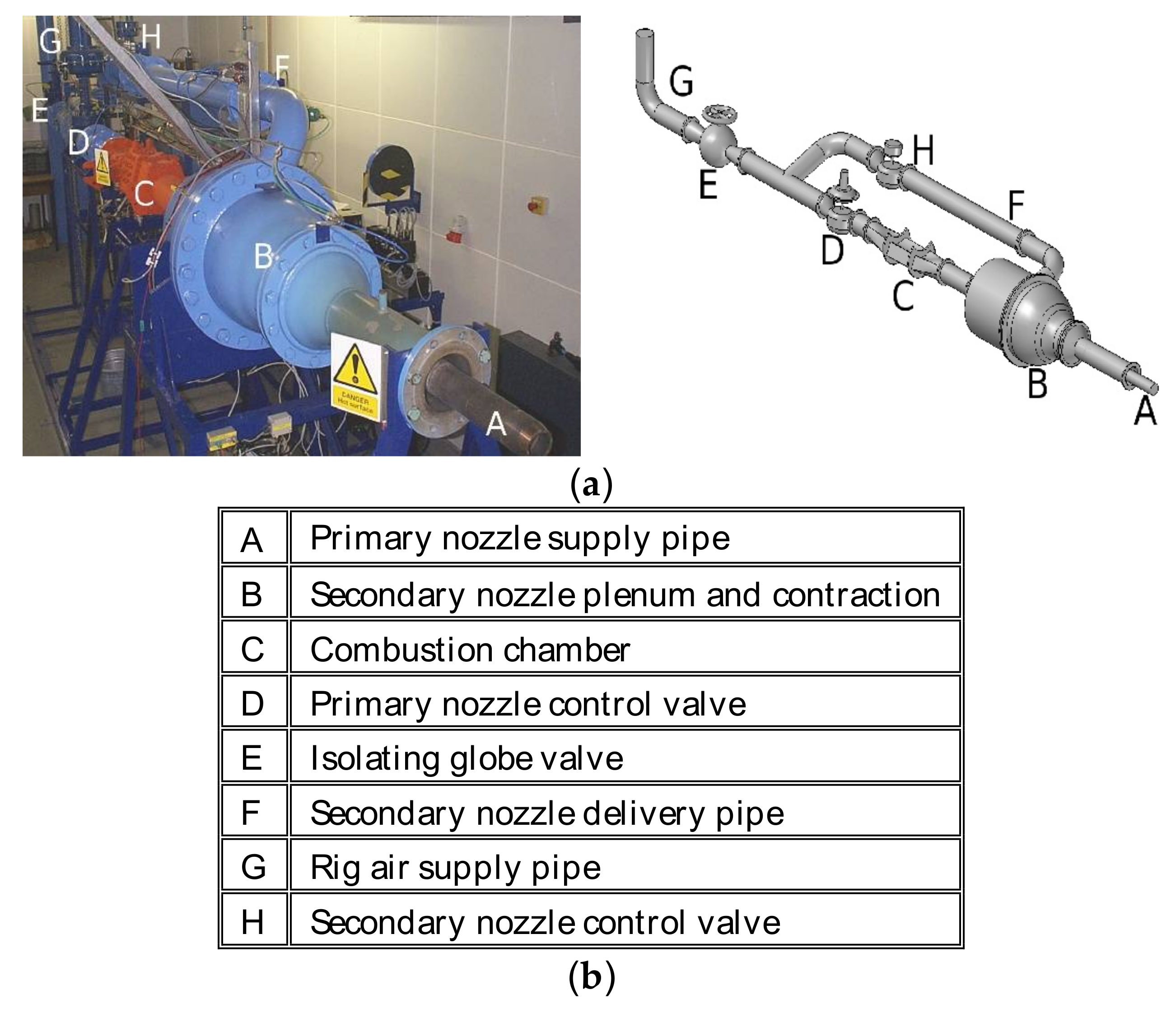
Figure 2.
Axisymmetric convergent test nozzles (dimensions in mm); D is nozzle exit diameter. (a) LU48; (b) LU60; (c) LU48P; (d) LU60P.
Figure 2.
Axisymmetric convergent test nozzles (dimensions in mm); D is nozzle exit diameter. (a) LU48; (b) LU60; (c) LU48P; (d) LU60P.

Figure 3.
(a) Nozzle inlet probe traverse arrangements; (b) Nozzle inlet total pressure profile LU60, NPR = 1.57.
Figure 3.
(a) Nozzle inlet probe traverse arrangements; (b) Nozzle inlet total pressure profile LU60, NPR = 1.57.

Figure 4.
(a) Nozzle exit dual head probe; (b) Nozzle exit probe traverse arrangement.

Figure 5.
(a) Nozzle exit total profile Near-wall, LU60, NPR = 1.58; (b) Nozzle exit total profile Full radius, LU60, NPR = 1.58.
Figure 5.
(a) Nozzle exit total profile Near-wall, LU60, NPR = 1.58; (b) Nozzle exit total profile Full radius, LU60, NPR = 1.58.

Figure 6.
Nozzle inlet boundary layer parameters: (a) Momentum thickness Reynolds number; (b) Momentum thickness; (c) Shape factor; (d) Skin friction coefficient.
Figure 6.
Nozzle inlet boundary layer parameters: (a) Momentum thickness Reynolds number; (b) Momentum thickness; (c) Shape factor; (d) Skin friction coefficient.

Figure 7.
Nozzle inlet mean velocity profile in log-law format. (a) Subsonic, LU60; (b) supersonic, LU48.
Figure 7.
Nozzle inlet mean velocity profile in log-law format. (a) Subsonic, LU60; (b) supersonic, LU48.

Figure 8.
Probe-measured nozzle exit momentum thickness (left) and shape factor (right). (a) LU48, θi; (b) LU48, H12i; (c) LU60, θi; (d) LU60, H12i.
Figure 8.
Probe-measured nozzle exit momentum thickness (left) and shape factor (right). (a) LU48, θi; (b) LU48, H12i; (c) LU60, θi; (d) LU60, H12i.

Figure 9.
LU60 nozzle inlet and exit velocity profiles (probe data).

Figure 10.
LU60 nozzle inlet and exit Clauser plots (probe and LDA data).

Figure 11.
LU48 nozzle exit shape factor H12i probe and LDA data.
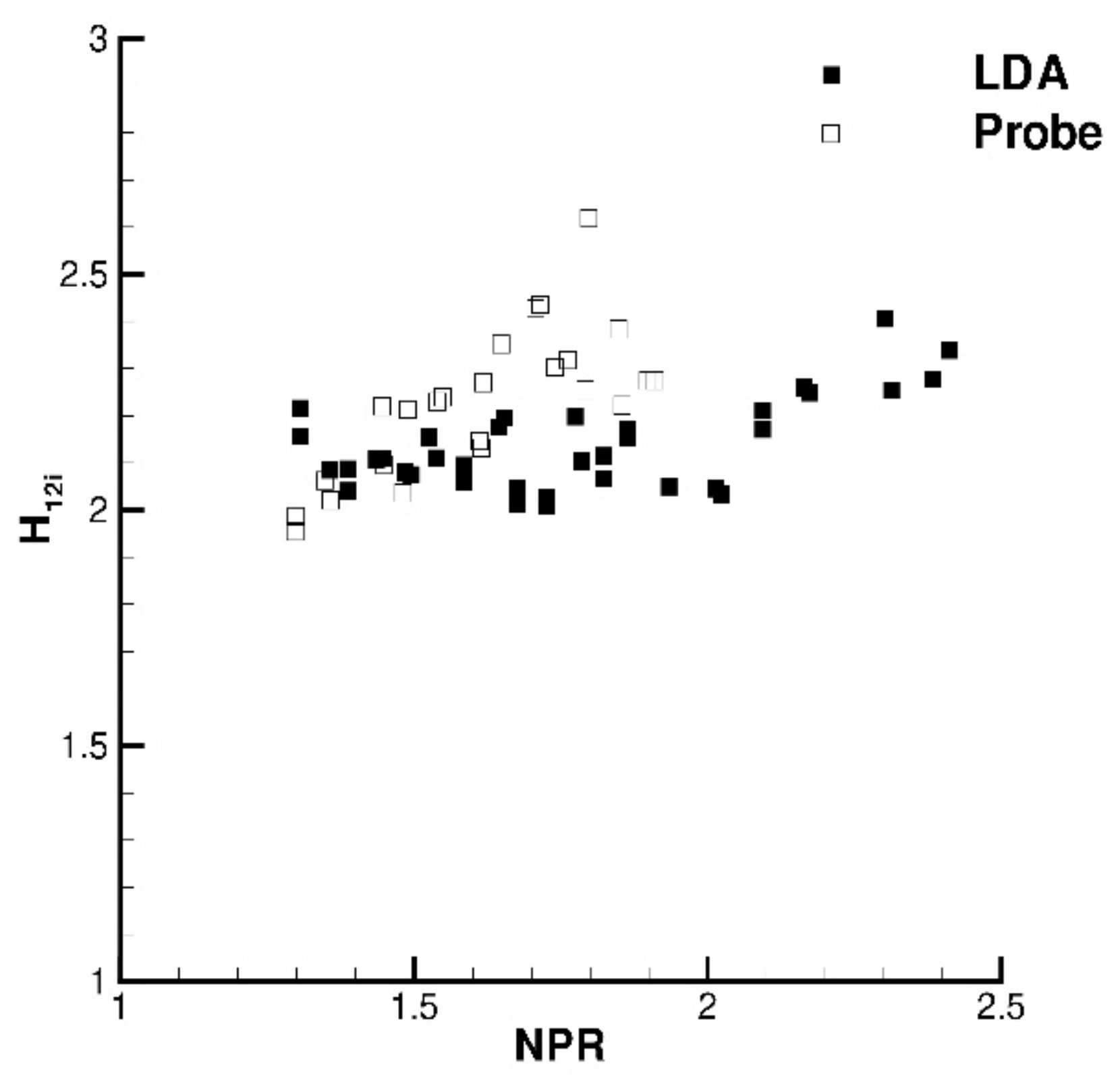
Figure 12.
LU48 nozzle exit profiles NPR = 1.77–2.41.

Figure 13.
LU60 nozzle exit LDA measurements, NPR = 1.8–2.4. (a) Axial rms turbulence; (b) Reynolds shear stress.
Figure 13.
LU60 nozzle exit LDA measurements, NPR = 1.8–2.4. (a) Axial rms turbulence; (b) Reynolds shear stress.

Figure 14.
LU60/LU60P nozzle exit axial velocity profiles.

Figure 15.
LU60 and LI60P nozzle exit Clauser plots.

Figure 16.
LU60/LU60P nozzle exit urms profiles.
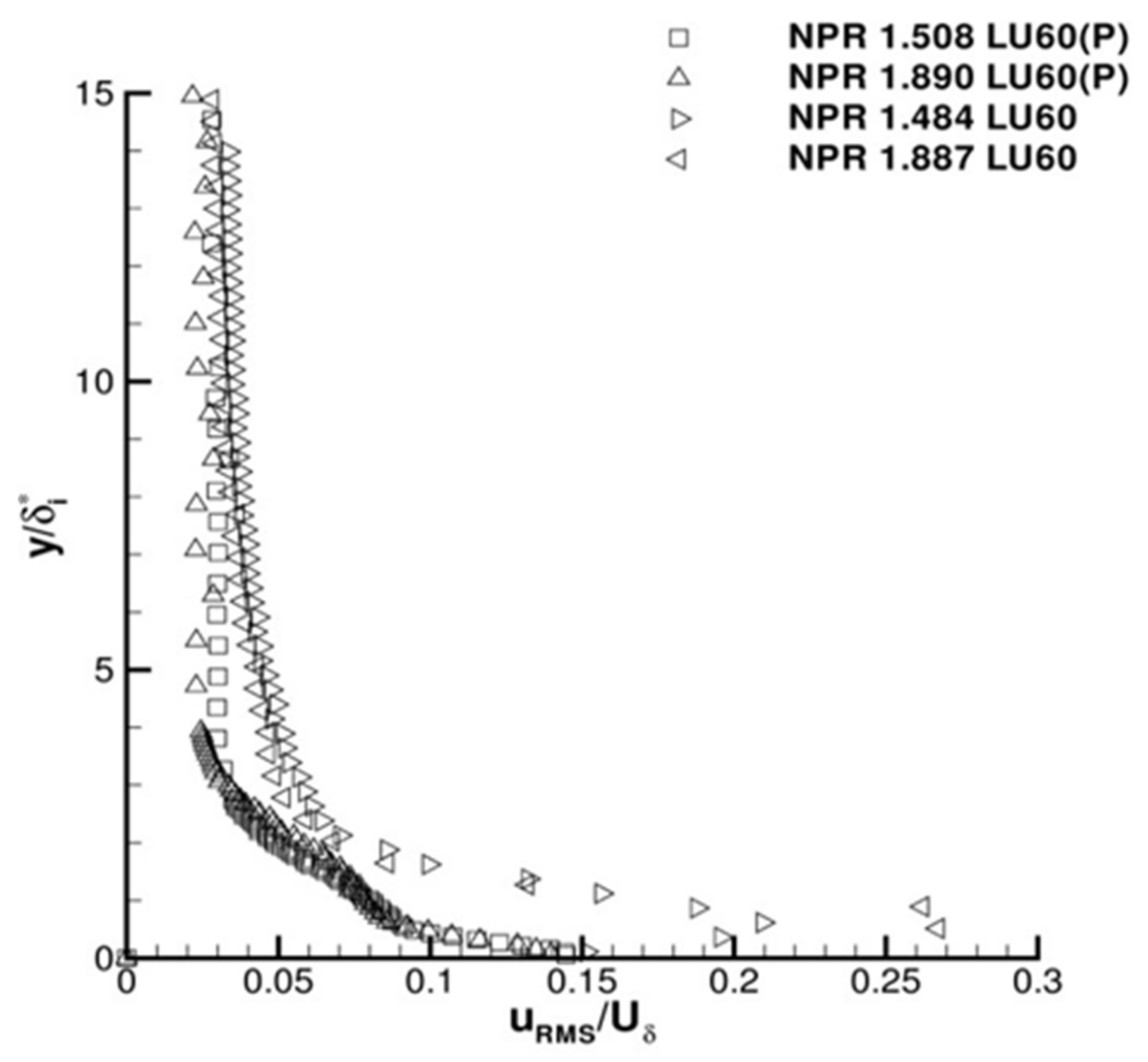
Figure 17.
LU60P nozzle exit shear stress profile.

Figure 18.
LU48/LU48P centreline and lipline profiles—NPR = 1.88. Top: centerline—(a) axial velocity; (b) axial rms turbulence. Bottom: lipline—(c) axial velocity; (d) axial rms turbulence.
Figure 18.
LU48/LU48P centreline and lipline profiles—NPR = 1.88. Top: centerline—(a) axial velocity; (b) axial rms turbulence. Bottom: lipline—(c) axial velocity; (d) axial rms turbulence.
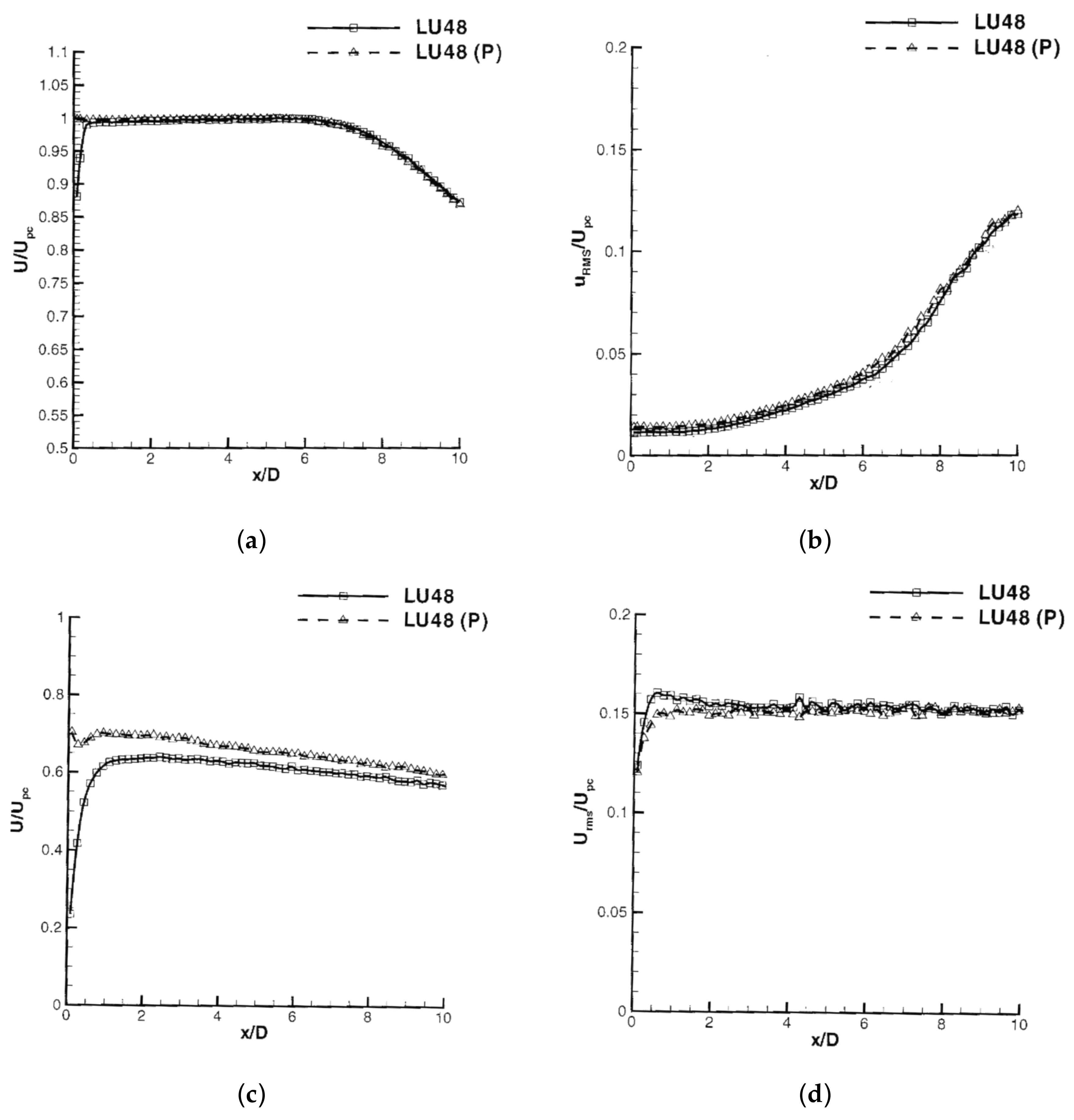
Figure 19.
LU48/LU48P centreline and lipline profiles—NPR = 2.40. Top: centreline—(a) axial velocity; (b) axial velocity (detail); Middle: centreline—(c) axial rms turbulence; (d) axial rms turbulence (detail). Bottom: lipline—(e) axial velocity; (f) axial rms turbulence.
Figure 19.
LU48/LU48P centreline and lipline profiles—NPR = 2.40. Top: centreline—(a) axial velocity; (b) axial velocity (detail); Middle: centreline—(c) axial rms turbulence; (d) axial rms turbulence (detail). Bottom: lipline—(e) axial velocity; (f) axial rms turbulence.
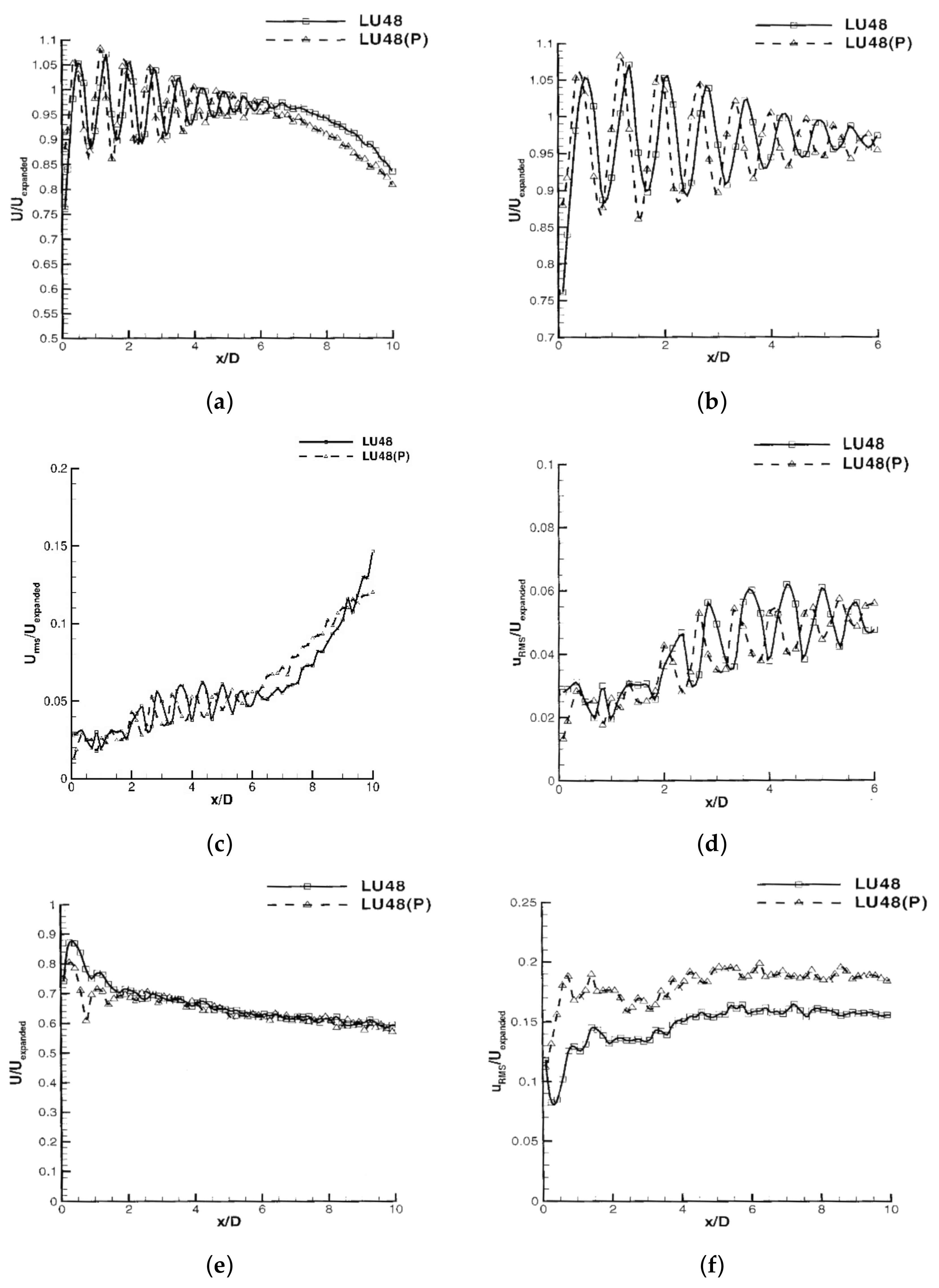
Figure 20.
Schlieren image for NPR = 2.40: (left) LU48P; (right) LU48.
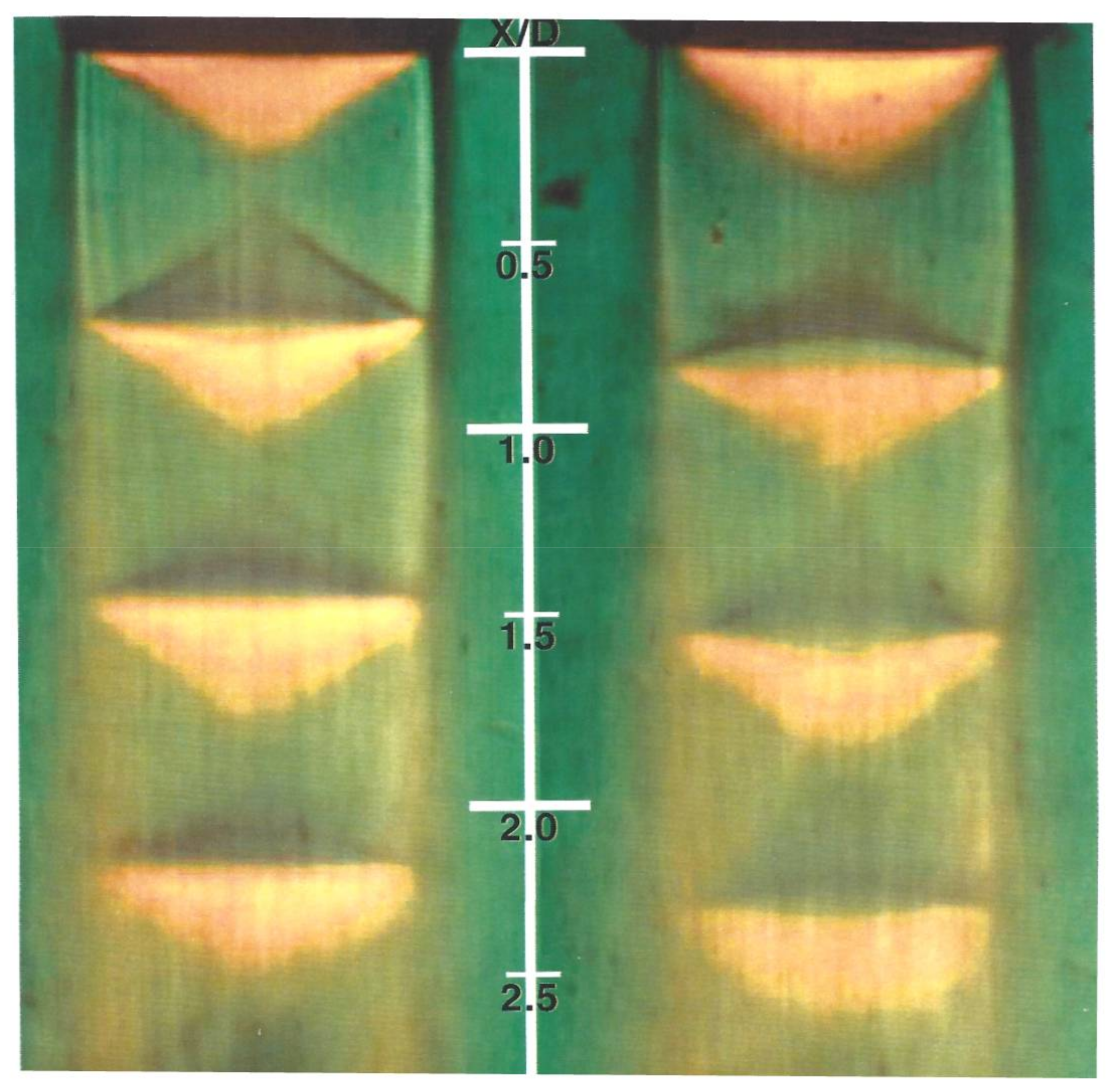
Figure 21.
Radial profiles: mean velocity (left), Reynolds shear stress (right), LU48/LU48P, NPR = 2.4. (a,b) x/D = 0.25 and 0.5; (c,d) x/D = 1.5 and 2.0; (e,f) x/D = 8.0.
Figure 21.
Radial profiles: mean velocity (left), Reynolds shear stress (right), LU48/LU48P, NPR = 2.4. (a,b) x/D = 0.25 and 0.5; (c,d) x/D = 1.5 and 2.0; (e,f) x/D = 8.0.


Table 1.
Optical parameters of LDA system.
| Beam Colour | L (mm) | θ (°) | s (μm) | Nf | dx (mm) | dy (mm) | dz (mm) |
|---|---|---|---|---|---|---|---|
| Green beam (λG = 514.5 nm) | 310 | 7.01 | 4.04 | 18 | 0.076 | 0.076 | 1.192 |
| Blue beam (λB = 488.0 nm) | 310 | 7.01 | 3.84 | 18 | 0.072 | 0.072 | 1.131 |
L = focal length; θ = 1/2 beam intersection angle; s/Nf = fringe spacing/no.; dx/dy/dz: measuring volume.
Table 2.
Effect of nozzle exit short parallel extension.
| Parameter | NPR = 1.50 | NPR = 1.88 | ||
|---|---|---|---|---|
| LU60 | LU60P | LU60 | LU60P | |
| θi (mm) | 0.0248 | 0.362 | 0.0177 | 0.239 |
| Reθi | 442 | 7494 | 430 | 6852 |
| H12i | 2.00 | 1.22 | 2.02 | 1.22 |
| (mm) | 0.065 | 0.44 | ||
© 2018 by the authors. Licensee MDPI, Basel, Switzerland. This article is an open access article distributed under the terms and conditions of the Creative Commons Attribution (CC BY) license (http://creativecommons.org/licenses/by/4.0/).
Share and Cite
MDPI and ACS Style
Trumper, M.T.; Behrouzi, P.; McGuirk, J.J. Influence of Nozzle Exit Conditions on the Near-Field Development of High Subsonic and Underexpanded Axisymmetric Jets. Aerospace 2018, 5, 35. https://doi.org/10.3390/aerospace5020035
AMA Style
Trumper MT, Behrouzi P, McGuirk JJ. Influence of Nozzle Exit Conditions on the Near-Field Development of High Subsonic and Underexpanded Axisymmetric Jets. Aerospace. 2018; 5(2):35. https://doi.org/10.3390/aerospace5020035
Chicago/Turabian StyleTrumper, Miles T., Parviz Behrouzi, and James J. McGuirk. 2018. "Influence of Nozzle Exit Conditions on the Near-Field Development of High Subsonic and Underexpanded Axisymmetric Jets" Aerospace 5, no. 2: 35. https://doi.org/10.3390/aerospace5020035
Note that from the first issue of 2016, this journal uses article numbers instead of page numbers. See further details here.