
Stochastic Trajectory Generation Using Particle Swarm Optimization for Quadrotor Unmanned Aerial Vehicles (UAVs)


EcoSys Lab, Alpen-Adria-Universität Klagenfurt, Universitätsstraße 65-67, 9020 Klagenfurt, Austria
*
Author to whom correspondence should be addressed.
Aerospace 2017, 4(2), 27; https://doi.org/10.3390/aerospace4020027
Submission received: 22 March 2017
/
Revised: 21 April 2017
/
Accepted: 4 May 2017
/
Published: 8 May 2017
(This article belongs to the Collection Unmanned Aerial Systems)
Abstract
:The aim of this paper is to provide a realistic stochastic trajectory generation method for unmanned aerial vehicles that offers a tool for the emulation of trajectories in typical flight scenarios. Three scenarios are defined in this paper. The trajectories for these scenarios are implemented with quintic B-splines that grant smoothness in the second-order derivatives of Euler angles and accelerations. In order to tune the parameters of the quintic B-spline in the search space, a multi-objective optimization method called particle swarm optimization (PSO) is used. The proposed technique satisfies the constraints imposed by the configuration of the unmanned aerial vehicle (UAV). Further particular constraints can be introduced such as: obstacle avoidance, speed limitation, and actuator torque limitations due to the practical feasibility of the trajectories. Finally, the standard rapidly-exploring random tree (RRT*) algorithm, the standard (A*) algorithm and the genetic algorithm (GA) are simulated to make a comparison with the proposed algorithm in terms of execution time and effectiveness in finding the minimum length trajectory.
1. Introduction
In the last decade, unmanned aerial vehicles (UAVs), mostly known as an autonomous aerial vehicles, have been used in numerous military, aerial photography, agricultural and surveillance applications. UAVs can be classified into three significant groups: fixed-wing UAVs, rotary-wing UAVs and hybrid-layout UAVs [1].
The advantages of fixed-wing UAVs are the high-speed and the ability to fly for long distances. However, mechanical systems for landing and take-off, for example the landing gear, have to be installed. Furthermore, spacious structures, e.g., landing strips, have to be built. In small areas with obstacles, vertical take-off and landing (VTOL) and the ability to hover in a motionless spot are crucial. Therefore, rotary-wing UAVs have more applications. In addition, VTOL UAVs have greater maneuverability in indoor flight. Hybrid-layout UAVs have both long distance flight and VTOL properties. On the other hand, they have complex mechanisms for changing from rotary wing to fixed wing during the flight.
Considering harsh scenarios characterized by limited area [2], the presence of obstacles and possible dynamic constraints, rotary-wing UAVs have been shown to give the best performance [3]. This is why we consider these specific types in this paper. In particular, a quadrotor UAV is assumed. Its model structure is depicted in Figure 1. The aim is to derive a model to represent realistic trajectories that such a UAV can follow. In particular, there exist several methods to generate trajectories, including splines [4], rational functions [5], polynomial [6] and Bézier curves [7,8]. Likewise, another technique for trajectory generation is to use analytical functions such as higher-order piecewise polynomials to represent the evolution of the position over time [9]. Also, there are remarkable works in which a collision-free path can be obtained using the standard rapidly-exploring random tree (RRT*) and sampling-based algorithms [10,11]. In order to provide a method that can represent the variability of the ensemble of flight trajectories followed by a UAV, it is of interest to define a stochastic approach. In this respect, the Confined Area Random Aerial Trajectory Emulator (CARATE) proposed in [12] stochastically generates a 3D path obtained from a variable length previous history of the trajectory and a tunable set of random variables. CARATE is specifically designed to emulate stochastic trajectories with a limited flight area. However, it does not consider the dynamics of the UAV and it is not optimized to cope with harsh environmental constraints. In this paper, we tackle the limitations above and we propose a novel stochastic trajectory generation method that: (1) takes into account the dynamics of a quadrotor UAV, and (2) copes with environmental limitations. To do this, the dynamic model of a quadrotor [13,14] is considered. Moreover, an analytic function (quintic B-spline) is used to generate candidate trajectories. Nonetheless, the disadvantage of the deterministic functions is that they are not able to satisfy all the constraints at the same time when planing the trajectory in the search space. Therefore, the genetic algorithm (GA) may be used to obtain an optimized trajectory [15]. Another approach uses swarm intelligence. In particular, particle swarm optimization (PSO) is based on a simple mathematical model, extended by Kennedy and Eberhart in 1995 [16], to describe the social behavior of birds and fish. PSO follows the basic principle of self-organization which is used to characterize the dynamics of complex systems. PSO uses a model of social behavior to unravel the optimization problems, in a cooperative and sagacious skeleton [17]. PSO is easy to apply and is powerful in solving a diverse range of multi-objective optimization problems where GA can not be used. Some other related papers based on particle swarm optimization for path planning include [18,19]. Our approach, on the other hand, enjoys a specific method for solving the optimization problem with constraints. We change the problem into one that considers a cost metric that includes a violation function. The constraints, namely position, velocity, acceleration, Euler angles, torques and obstacle avoidance are added in the violation function.
To validate the proposed method, three scenarios are defined:
- Flight level (FL) trajectory;
- Take-off → Mission → Landing (TML);
- Complex maneuvering in 3D space (CMS).
In each scenario, random trajectories are generated under certain constraints that can be imposed with the given initial point (IP) and target point (TP) in three-dimensional coordinates.
We organize the contents of this paper as follows. Section 2 describes the world frame, body frame, dynamic model and the kinematics of the quadrotor. The trajectory modeling approach and the description of the three considered scenarios is given in Section 3. In Section 4, we define the cost function and the violation function related to the constraints and obstacle avoidance. Finally, examples of realized trajectories are reported in Section 5. The conclusions follow.
2. Dynamic Model
In order to represent the dynamic model of a quadrotor, two coordinate systems will be introduced. They describe the orientation and the motion of a quadrotor in the world frame and in the body frame. The world frame is referred to as the inertial earth coordinate (north east down, NED) system. As can be observed in Figure 1, the earth is assumed to be fixed. Therefore, the inertial earth frame can be defined. The body coordinate o system is installed at the quadrotor’s center of gravity (CoG). Each frame follows the right hand rule [20]. The notations used in this paper are reported in Table 1.
The Euler angles are used to represent the orientation of the quadrotor which is considered as a point mass, with respect to a fixed reference frame (body frame). The euler angle rates can be represented in matrix form as follows [21]:
The direction cosine matrix that allows to obtain a transform from the body frame to the world frame is denoted with . Hence, consists of three sequential single-axis rotations through the basic Euler angles , and that represent the roll, pitch and yaw, respectively. The direction cosine matrix can be obtained according to the relations below [22]:
2.1. The Moment of Inertia
In this paper, the quadrotor is assumed to be a symmetric body. To define the moment of inertia, we assume the quadrotor to consist of four rotors and a main body. The main body is a sphere with radius R and a mass M. The four rotors are assumed to be a point mass . Then, the point masses are connected to the center of the sphere with radius l. Therefore, the inertia matrix is a diagonal symmetric matrix:
with,
2.2. Thrust and Torques
The translational position, velocity and acceleration of the point mass o represented in the inertial frame , are:
According to Figure 1 the speed of each propeller can affect the motion of the quadrotor, so the relation between the thrust and torque generated by each rotor can be expressed as follows [13]:
while b and d are coefficients related to the Mach number, the Reynolds number and the angle of attack. Also, the input torques can be defined by:
2.3. Dynamic Model
The dynamic model of the quadrotor can be defined [13,14] according to the following relations:
where,
In Equation (15), , and are equal to:
The inverse kinematics of our model that are referred to as control inputs of the quadrotor according to Equation (15) are:
Indeed, the quadrotor has four motors actuating the four rotors while our system has six degrees of freedom. It can be deduced that our system is underactuated. In order to resolve the issue, we have to identify the dependency in Equation (15), as proposed by [23]:
Equation (19) shows two nonholonomic constraints existing in the kinematics of the quadrotor. Therefore, the angles and can be derived from these nonlinear equations:
The input torques can be obtained by the actuators of the quadrotor. Exploiting Equation (20), we can define the fitness function and boundary conditions in our model by evaluating , for and its time derivatives. We refer to as the trajectory evolution.
3. Modeling of Three Representative Scenarios
Our goal is to develop a stochastic model for the trajectory evolution. Indeed, at a first glance this can appear a difficult task since the UAV can follow a number of different trajectories and be in various flying situations. Therefore, we propose to consider certain scenarios that can be representative of certain flying operations. In each scenario, the trajectory evolution is represented with a B-spline drawn from a certain random model. In more detail (Figure 2), the B-spline has order k and it is defined by control points [4]. In our model, the first and the last control point are fixed and they correspond to the start and the end of the mission, respectively. In the search space between these two points, additional control points are placed in order to generate the segments of the B-spline curve. Each one of the control points is defined with coordinates in the search space, which are and each of them is generated stochastically as a uniform random variable ranging between a lower and an upper limit that are distributed over time by the user. This configuration enables a stochastic behaviour for . Indeed, by changing the location of the control points in the search space, a new path can be realized.
The mathematical model for a B-spline curve of degree k is defined by:
where are control points and are the basis functions defined using the Cox-de Boor recursion formula [4]:
The reason for using the B-spline is that unlike the global property of the Bezier curve, it has the local property [24]. Furthermore, the order of the B-spline is very important to generate feasible trajectories that fulfill constraints and obtain trajectory continuity and smoothness. To do so, we use fourth-order B-splines (quadratic) and fifth-order B-splines (quintic) in the considered scenarios.
3.1. Scenario One (FL)
3.2. Scenario Two (TML)
In all kind of UAVs, take-off, mission and landing (TML) are crucial. The challenge in modeling this scenario is the tuning of the parameters of the B-spline in a way that: (1) the velocity profiles of the trajectories during take-off and landing are zero (rest-to-rest manoeuvre); (2) the absolute value of the velocity should be less than 1.5 m/s; (3) the Euler angles during take-off and landing are zero (rest-to-rest manoeuvre); and (4) the quadrotor reaches the specific altitude (10 m) during the flight time. Clearly, other constraints can be defined. For simplicity, the surface of the ground is assumed to be horizontal. The length and duration of the trajectory between take off and landing can be made variable. Further details about modeling this scenario are reported in Section 4 and numerical examples in Section 5.
3.3. Scenario Three (CMS)
The third considered scenario highlights the ability of our approach to model trajectories that comprise obstacle avoidance procedures. Static obstacles with different size can be defined in the flight space. In particular, we consider three obstacles. Finding a safe and short trajectory in the search space with obstacles becomes a challenging problem in path planning. On the other hand, according to the configuration of our quadrotor, the feasibility of these trajectories is also significant. Boundary constraints for complex maneuver in 3D space are defined in Equation (25). More details are reported in Section 5.
4. Trajectory Realization under Practical Constraints
As discussed previously, the trajectory evolution is with input controls . Also, the dynamics of a quadrotor and environmental constraints add mathematical constraints to the generation of feasible quadrotor trajectories. In the following discussion, the constraints will be defined. Therefore, our problem is to determine the optimal coefficients of the B-spline under particular constraints. The boundary constraints in our scenarios are:
where is the minimum Euclidian distance between the UAV and a given a generic obstacle. It means that for , the UAV will not crash during the flight. We solve this problem with the PSO algorithm in Section 4.2.
4.1. Design of Trajectory with Minimum Length
The aim of this paper is generating stochastic trajectories. However, in path planning when the search space is populated with generic obstacles, finding the short and safe path among these trajectories becomes significant. We can therefore consider the problem of designing the shortest path trajectory. This translates into the definition of a cost function that equals the length of the path as follows:
where we have discretized the time evolution so that the coordinates at time instant i are denoted with and the sampling period is T. Our problem is a multi-objective optimization problem that has a cost function with boundary constraints. To proceed, we write it as a problem without constraints, however it includes a violation function to obtain the new cost function.
where N denotes the total number of samples considered in the overall trajectory. i represents the time index. J is the cost function that is equal to the length of the path. is the violation at time i for constraint . The constraints are the position, velocity, acceleration, Euler angles, torques and obstacle avoidance. Two important properties for the violation function are and . In order to satisfy the boundary constraints in Equation (25), the violation function for less, more and equal constraints can be defined respectively as follows:
where refers to a certain constraint as already explained. In addition, and represent the physical quantity and target constraint respectively. Now with the violation functions definition in Equation (28), the boundary conditions in Equation (25) can be satisfied. For obstacle avoidance, the Euclidian distance between the edge of the object and the quadrotor is used [26]. The whole algorithm is sketched in Figure 3.
4.2. Basics of PSO
Particle swarm optimization (PSO) is an intelligent optimization algorithm. It belongs to the class of algorithms called metaheuristics. PSO is based on the paradigm of swarm intelligence and it is inspired by social behavior of animals like fish and birds [16]. PSO is a simple yet powerful optimization algorithm and it is successfully applied to multiple applications in various fields of science and engineering like machine learning, mesh processing, data mining and many other fields.
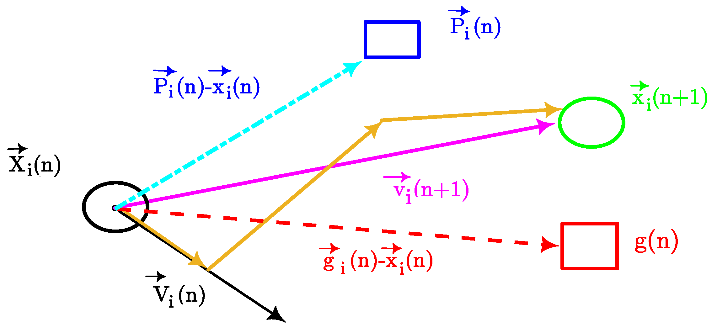
PSO contains a population of candidate solutions called a swarm. According to Figure 4, every particle is a candidate solution to the optimization problem. Any particle has a position in the search space of the optimization problem. The search space is the set of all possible solutions to the optimization problem. PSO allows for efficiently finding an optimal solution under a target function with multiple constraints in the problem at hand.
To proceed, we consider particles for the position vector and the velocity vector . Therefore, the updating realization for the particles includes [16]:
where i denotes the time index. is the particle index, and L is the number of considered particles. , and are real valued coefficients. is the personal learning coefficient and is the global learning coefficient. w is an inertial coefficient. and are acceleration coefficients. On the other hand, , are random numbers uniformly distributed in the range from zero to one (, ). is the best personal position of the particle of index n at time i, while is the best collective position of all particles at time i in the swarm. It should be noted that in the original version of PSO proposed in 1995, there was no inertia term. However, in 1998 Shi and Eberhart added the inertia term to the standard PSO [27].
5. Numerical Generator and Results
In this section, first we report a summary of example parameters to be used to generate trajectories in the three considered scenarios. The proposed algorithm can be used for any configuration of UAVs, but herein, we focus on a quadrotor. A number of parameters is initially fixed as shown in Table 2 [13]. Furthermore, in each flight scenario the start point, end point and a number of control points are defined by the user. We also report the number of particles and the number of iterations run by the PSO for the generation of trajectories with a certain number of control points. The details for each scenario are given in Table 3. The number of iterations listed in Table 3 to obtain the minimum length path are needed for the convergence. The average cost metric as a function of the iterations will be shown in Section 5.1, Section 5.2 and Section 5.3 for Scenarios 1, 2 and 3, respectively. The execution time has been computed for a simulation setup with an Intel i5 CPU with 3.3 GHz, and RAM of 4GB using MATLAB 2016b. Finally, we demonstrate the performance of our method in comparison with the standard (A*) algorithm, the standard rapidly-exploring random tree (RRT*) algorithm and the genetic algorithm (GA) for obtaining the minimum length path in 2D.
5.1. Scenario 1 (FL)
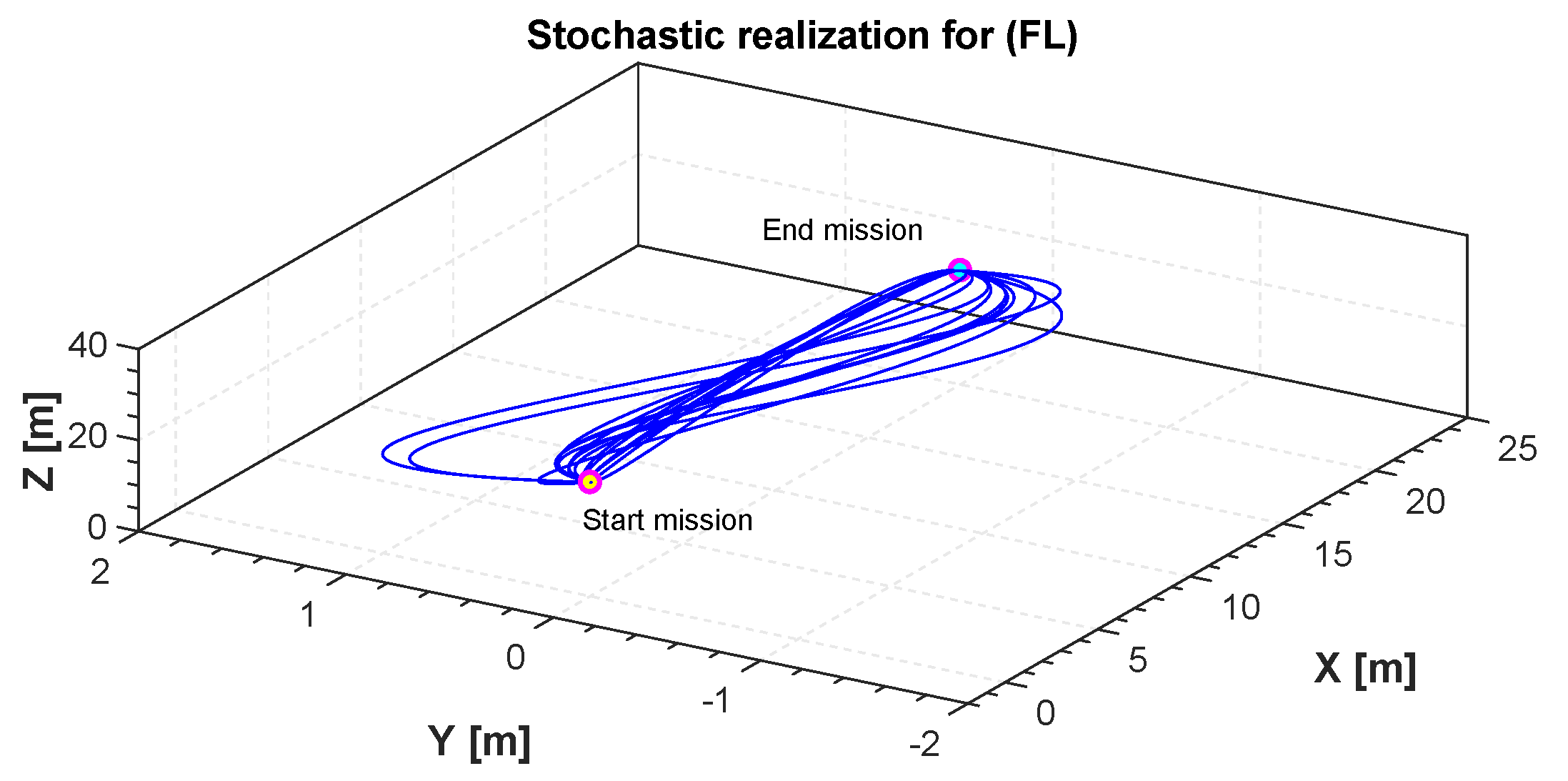
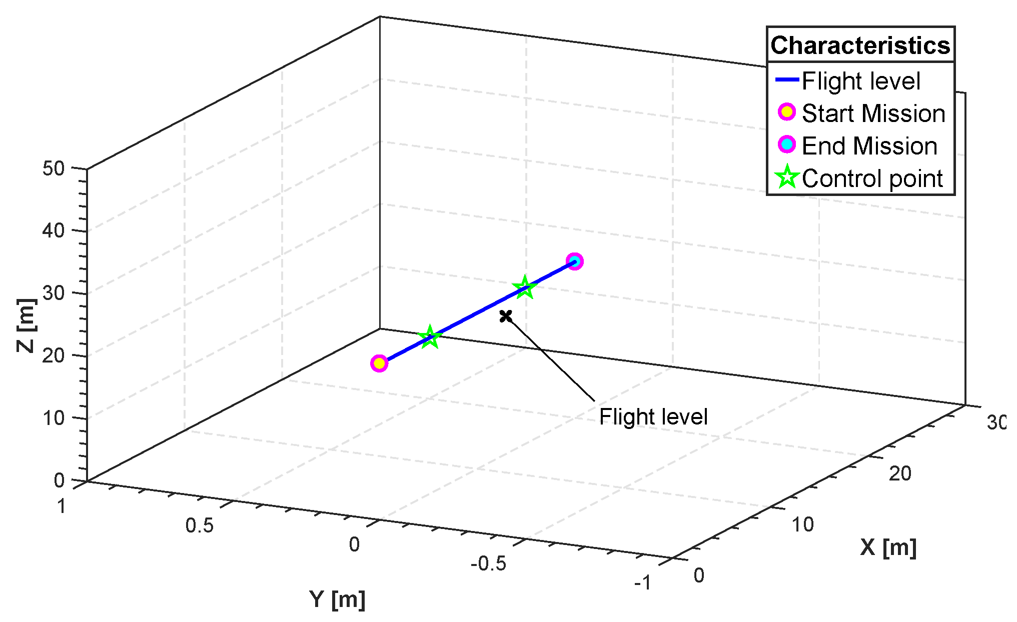
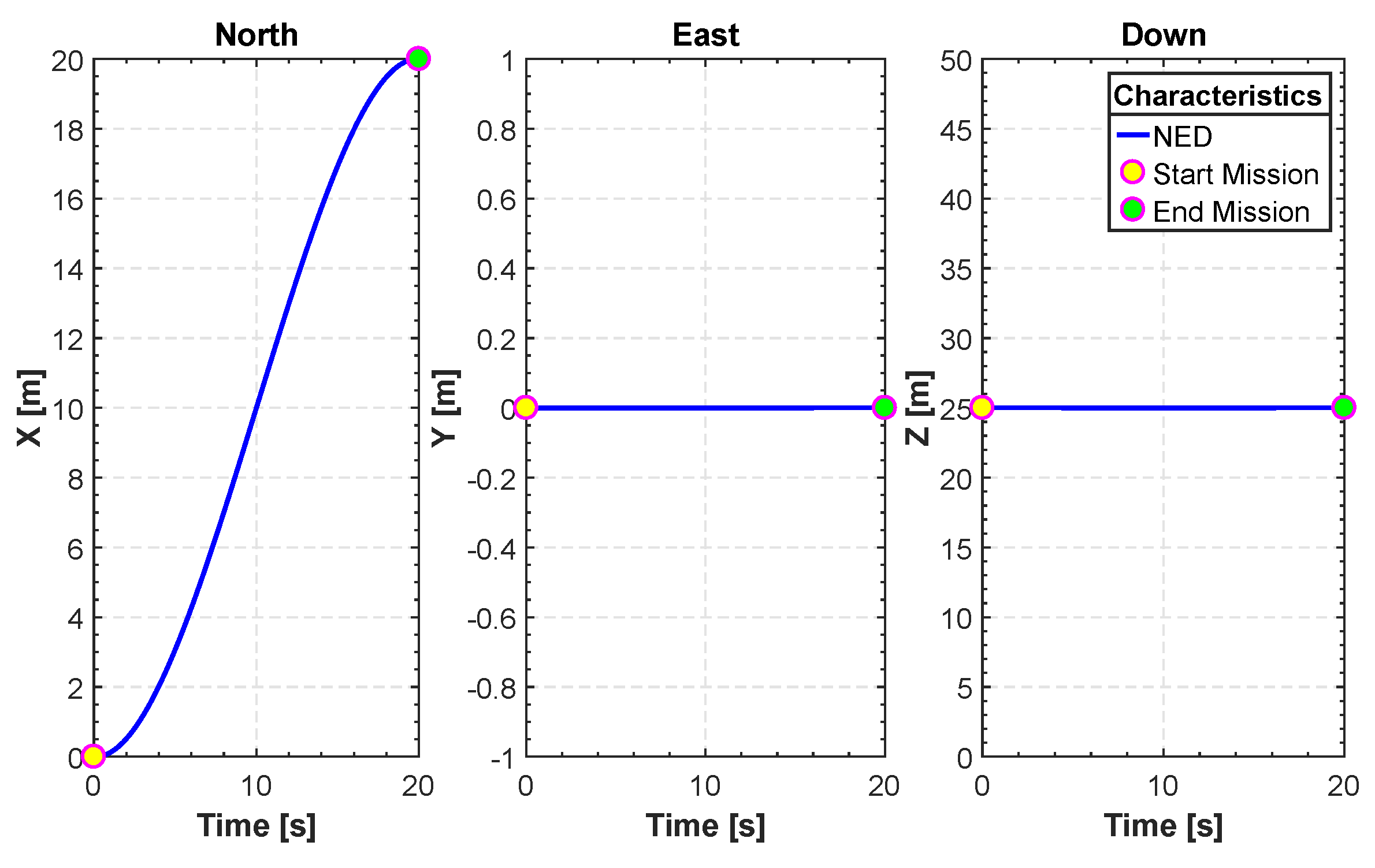
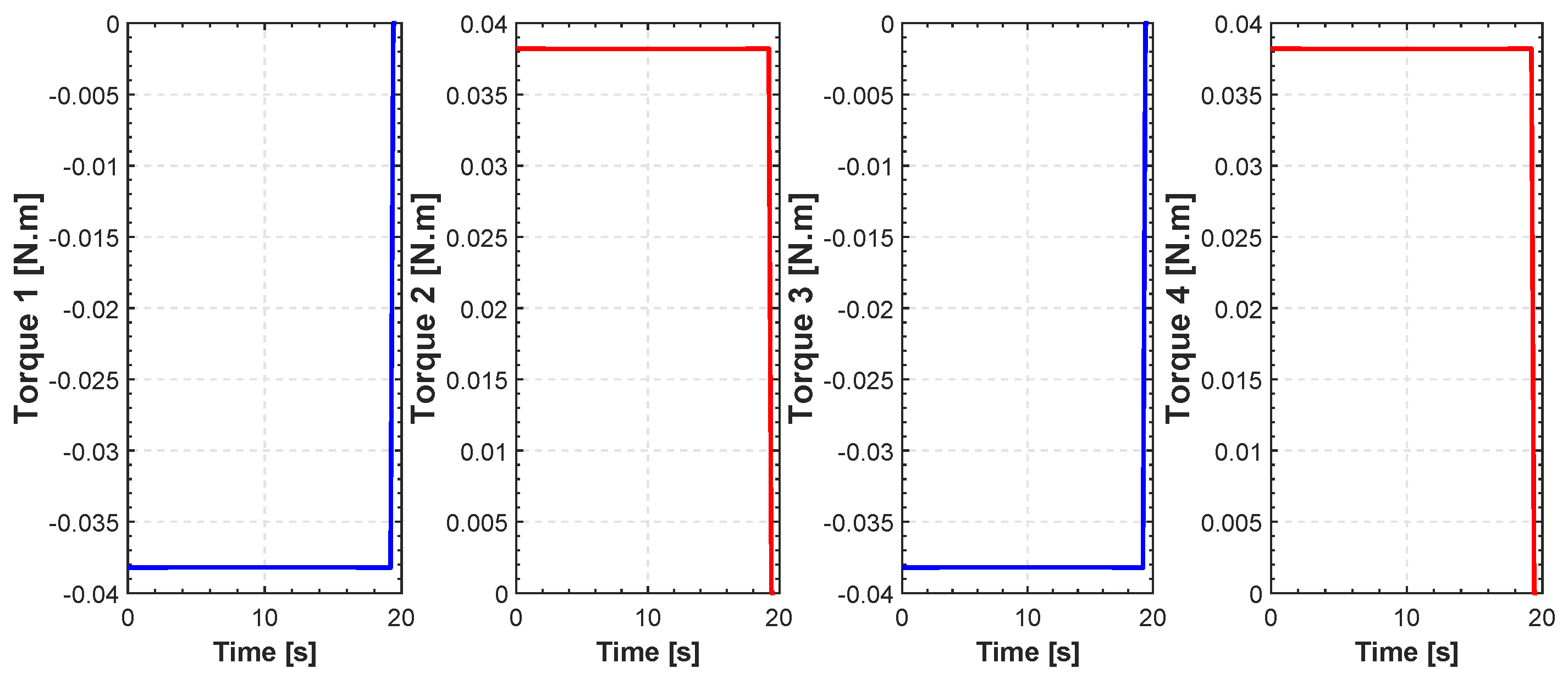
Figure 5 shows a number of realizations of possible trajectories generated by the algorithm. Among these trajectories one is chosen based on the constraints set in Equation (25) in order to isolate the one with least distance. The initial and final position can be chosen by the user. In this specific example the initial position of our quadrotor is in meters. The final position is . The fourth-order B-spline is considered for this scenario. Figure 6 shows the minimum length trajectory that is obtained from the PSO. Furthermore, the details about positions, actuators torques, control efforts, translational velocities and the acceleration obtained with the PSO are given in Figure 7, Figure 8, Figure 9 and Figure 10. Figure 11 shows the average cost metric (Equation (27)) as a function of iterations. The convergence is achieved in about 250 iterations. PSO algorithm converges quickly to the optimal solution. The minimum length of the trajectory for this scenario obtained via simulation is m and the total flight time is 20 s.
5.2. Scenario 2 (TML)
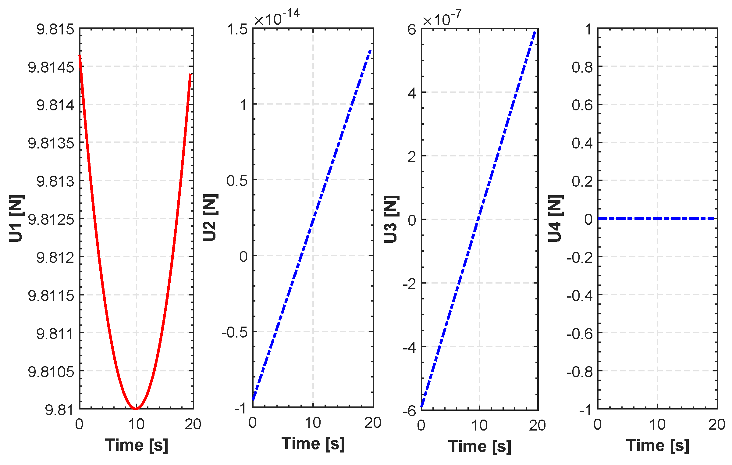
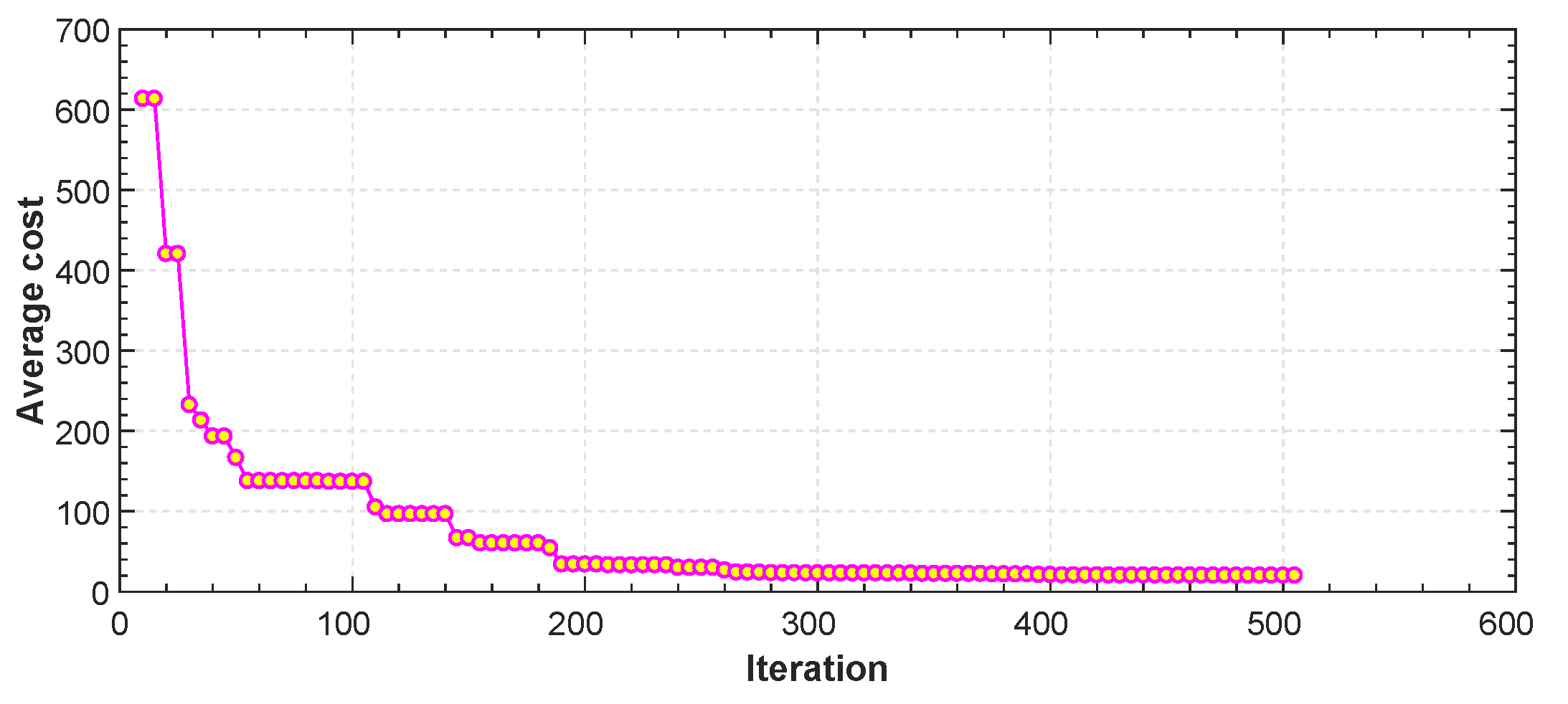
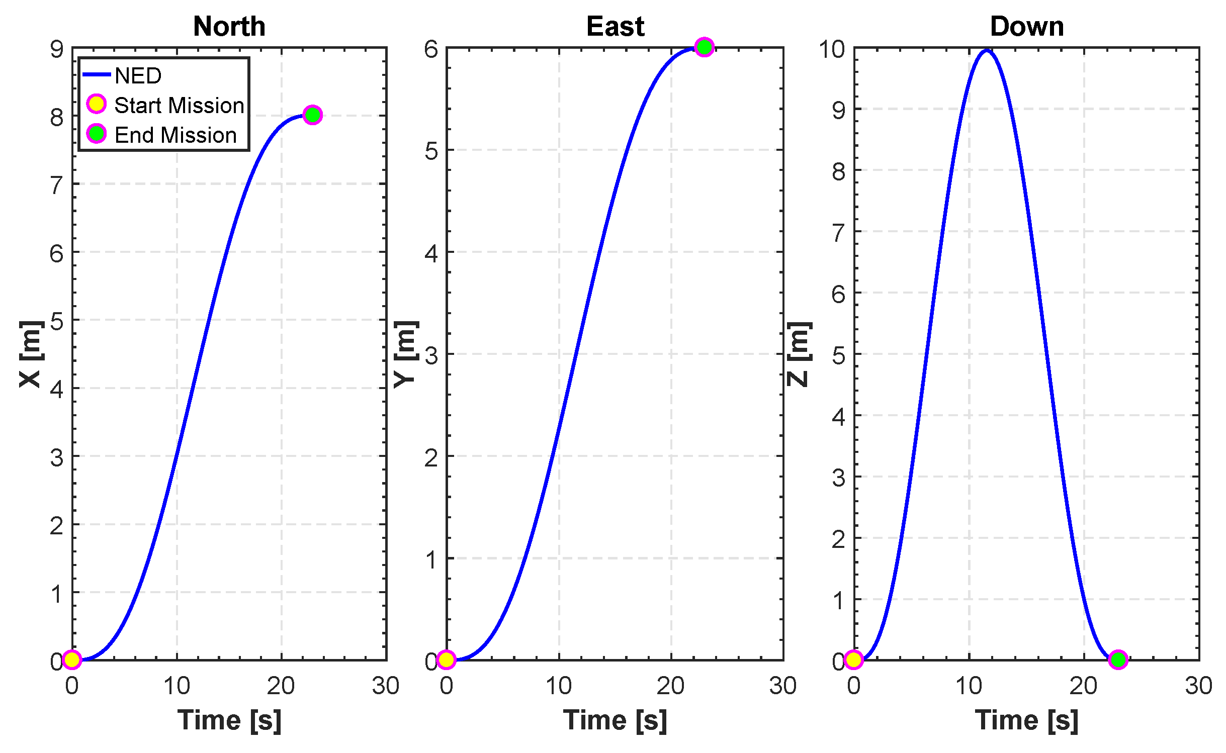
In Figure 12, Figure 13, Figure 14, Figure 15 and Figure 16, we report an example of trajectory belonging to the Scenario 2 (TML). In particular, the starting point is and the landing point is . The maximum altitude during the flight time is 10 m. Also, Figure 17 shows the minimum length trajectory (J = 33.9608 m) which is obtained after 100 iterations of the PSO algorithm. Figure 15 represents the inertial frame for the velocity components, which are less than 1.5 m/s according to our constraints definition in scenario two and the total flight time is 23 s.
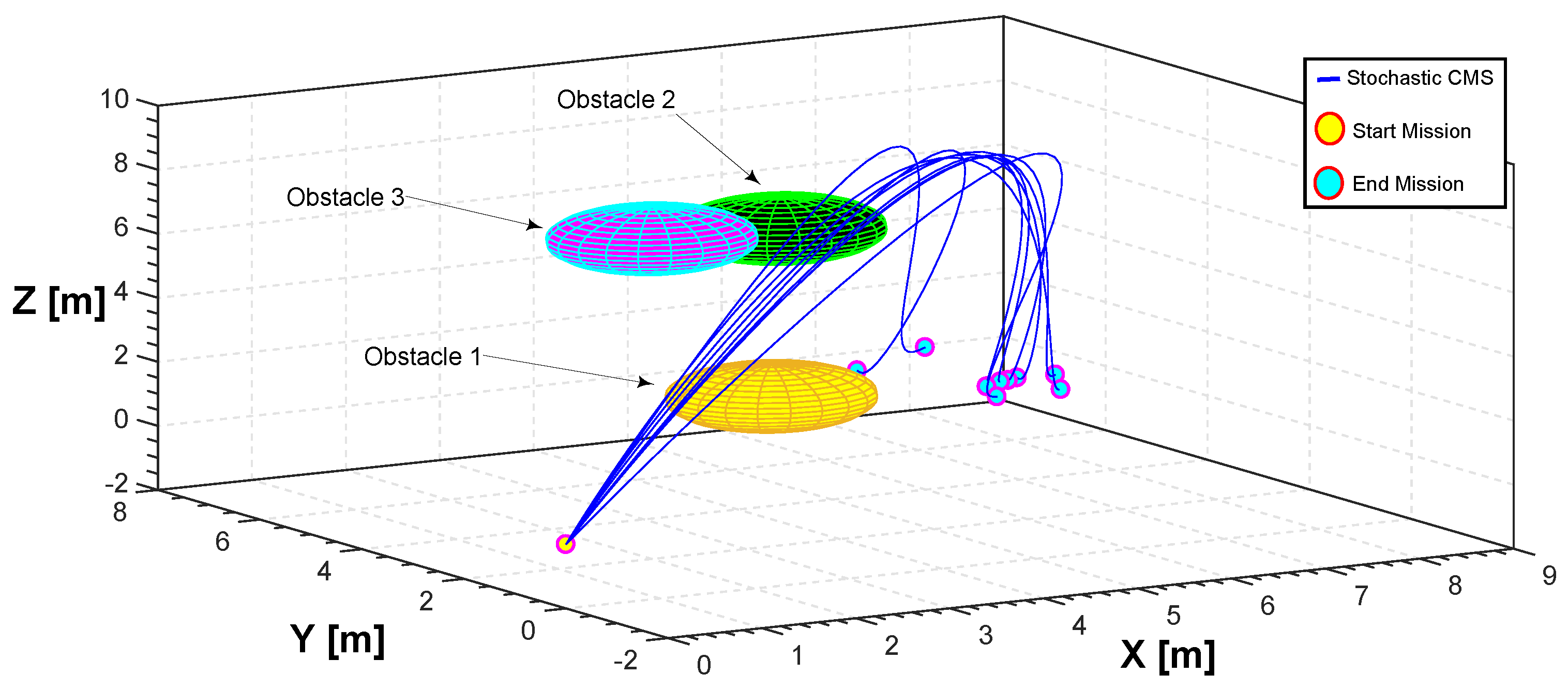
5.3. Scenario 3 (CMS)
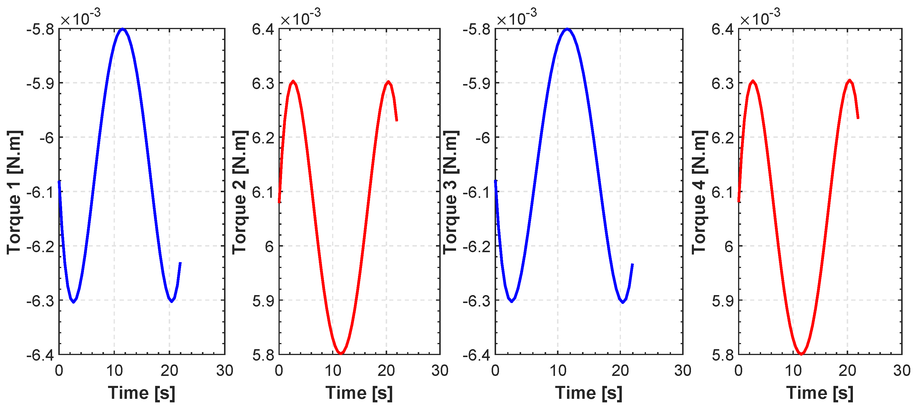
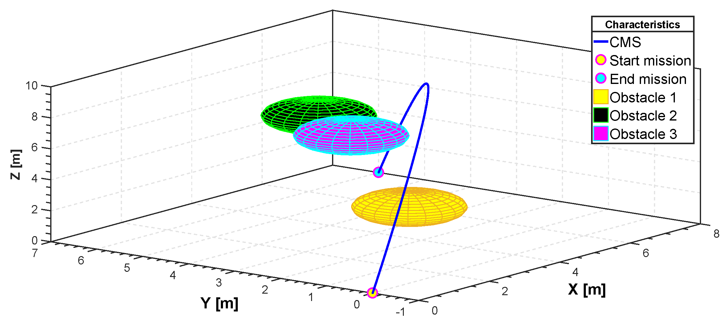
In Figure 18, the search space is populated with three generic spherical objects that act as obstacles for the quadrotor and thus hinder their path. These obstacles can be either positioned arbitrarily by the user or randomly generated by the algorithm. In this specific case they were generated by the user. For CMS, a stochastic realization as a set of trajectories is shown in Figure 18. The start point is and the end point is . Simulation results for the cost function and the actuator torques are shown in Figure 19 and Figure 20. Also, the minimum path after 150 iterations and the total flight time are , and 23 s, respectively. Furthermore, the minimum length path obtained with PSO and time histories of the attitude angle of the quadrotor are shown in Figure 21 and Figure 22, respectively.
5.4. PSO vs. A*, RRT* and GA
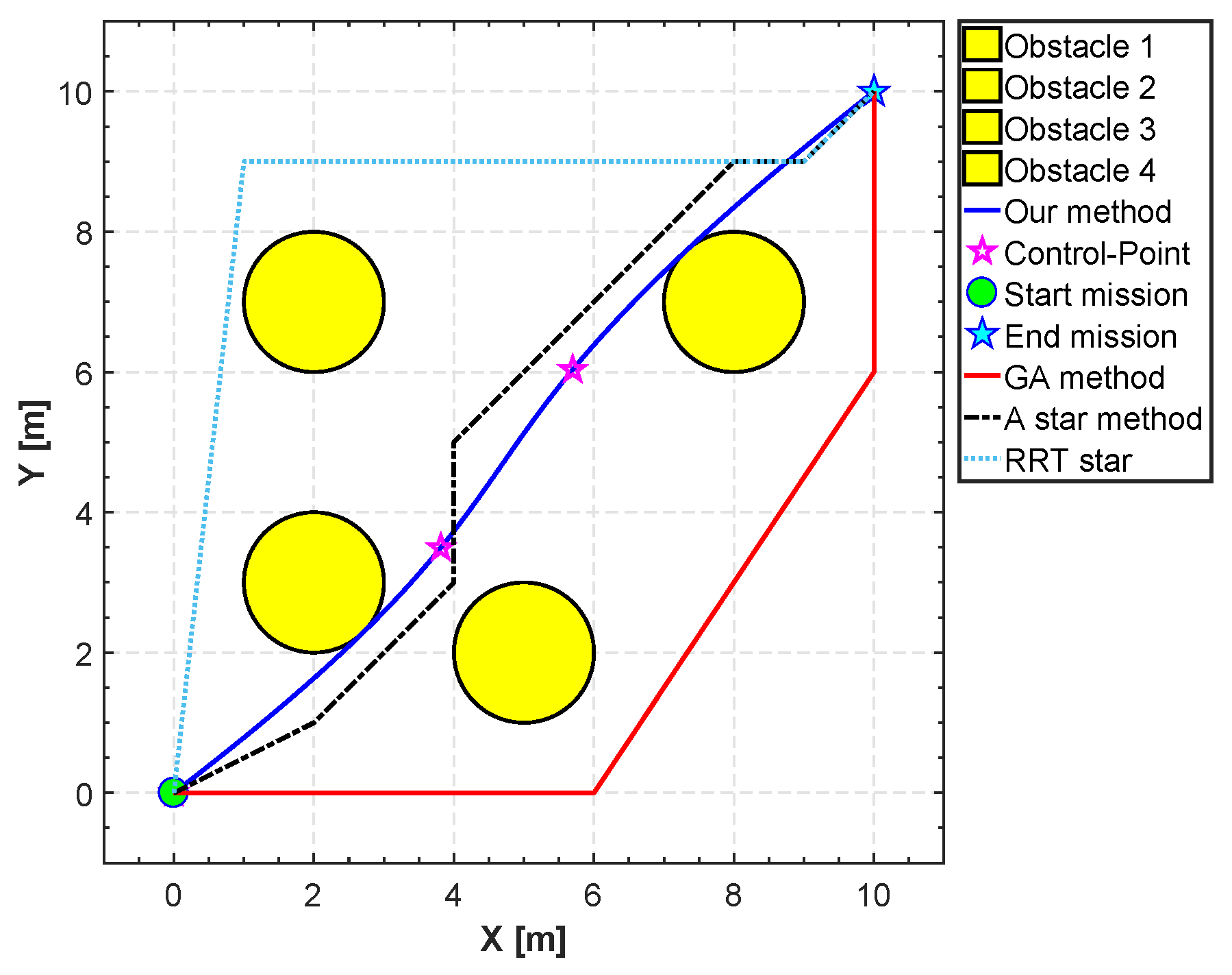
As already mentioned before, to illustrate the effectiveness of the proposed method, we consider three different methods named the RRT* algorithm, the A* algorithm and the GA to obtain the minimum path in 2D that obeys several constraints. The search space is also surrounded by four obstacles. As shown in Table 4 and Figure 23, the results for the proposed method show that it has a faster convergence time and it finds a path with smaller length and collision avoidance. The optimum length for our method is 14.2095 m. Also, it is noticeable that the execution-time for the A* algorithm is 0.02315 s. The execution time does not consider the part for the construction of the B-spline curves.
6. Conclusions
In this paper, a new methodology has been proposed for stochastic modeling and generating trajectories followed by a UAV. The approach is based, firstly, on modeling a certain flight scenario. Then, the evolution of the trajectory is obtained using a B-spline with a certain order and setting some control points. A PSO multi-objective optimization algorithm is used to not only tune the parameters of the B-spline function, but also to guarantee that the trajectories are dynamically feasible. The trajectories can also model an obstacle avoidance situation. This has been realized by defining a violation function to avoid collision during the flight time with obstacles at certain positions. A numerical simulator has been implemented to emulate the reference scenarios. The simulator can be configured to allow variability and representativity of the flight scenario. Several trajectory examples have been shown to verify the trajectory smoothness and fulfillment of practical constraints introduced by the UAV dynamics.
Author Contributions
Babak Salamat developed the UAV trajectory optimization procedure under feasibility constraints, obtained the numerical results and prepared the paper. Andrea M. Tonello conceived the overall UAV random trajectory generation concept, supervised the development of the model, results and paper.
Conflicts of Interest
The authors declare no conflict of interest.
References
- Austin, R. Unmanned Aircraft Systems: UAVS Design, Development and Deployment, 1st ed.; Wiley: Chichester, UK, 2010. [Google Scholar]
- Majka, A. Trajectory Management of the Unmanned Aircraft System (UAS) in Emergency Situation. Aerospace 2015, 2, 222–234. [Google Scholar] [CrossRef]
- Suicmez, E.C.; Kutay, A.T. Optimal path tracking control of a quadrotor UAV. In Proceedings of the 2014 International Conference on Unmanned Aircraft Systems (ICUAS), Orlando, FL, USA, 27–30 May 2014; pp. 115–125. [Google Scholar]
- Sprunk, C. Planning Motion Trajectories for Mobile Robots Using Splines; Student Project; University of Freiburg: Freiburg, Germany, 2008. [Google Scholar]
- Montés, N.; Mora, M.C.; Tornero, J. Trajectory Generation based on Rational Bezier Curves as Clothoids. In Proceedings of the IEEE Intelligent Vehicles Symposium, Istanbul, Turkey, 13–15 June 2007; pp. 505–510. [Google Scholar]
- Babel, L. Three-dimensional Route Planning for Unmanned Aerial Vehicles in a Risk Environment. J. Intell. Robot. Syst. 2013, 71, 255–269. [Google Scholar] [CrossRef]
- Jayasinghe, J.A.S.; Athauda, A.M.B.G.D.A. Smooth trajectory generation algorithm for an unmanned aerial vehicle (UAV) under dynamic constraints: Using a quadratic Bezier curve for collision avoidance. In Proceedings of the 2016 Manufacturing Industrial Engineering Symposium (MIES), Colombo, Sri Lanka, 22 October 2016; pp. 1–6. [Google Scholar]
- Tsai, Y.J.; Lee, C.S.; Lin, C.L.; Huang, C.H. Development of Flight Path Planning for Multirotor Aerial Vehicles. Aerospace 2015, 2, 171–188. [Google Scholar] [CrossRef]
- Cruz, A.B.; Montaño, J.C.; Mier, P.G. TG2M: Trajectory Generator and Guidance Module for the Aerial Vehicle Control Language AVCL. In Proceedings of the 40th International Symposium on Robotics, Barcelona, Spain, 10–14 March 2009. [Google Scholar]
- Karaman, S.; Frazzoli, E. Sampling-based algorithms for optimal motion planning. Int. J. Robot. Res. (IJRR) 2011, 30, 846–894. [Google Scholar] [CrossRef]
- Barbehenn, M. A note on the complexity of Dijkstra’s algorithm for graphs with weighted vertices. IEEE Trans. Comput. 1998, 47, 263. [Google Scholar] [CrossRef]
- Papaiz, A.; Tonello, A. Azimuth and Elevation Dynamic Tracking of UAVs via 3-Axial ULA and Particle Filtering. Int. J. Aerosp. Eng. 2016, 2016, 1–9. [Google Scholar] [CrossRef]
- Sanca, A.S.; Alsina, P.J.; Cerqueira, J.J.F. Dynamic Modelling of a Quadrotor Aerial Vehicle with Nonlinear Inputs. In Proceedings of the 2008 IEEE Latin American Robotic Symposium, Salvador, Bahia, Brazil, 29–30 October 2008; pp. 143–148. [Google Scholar]
- Mohammadi, M.; Shahri, A.M. Modelling and decentralized adaptive tracking control of a quadrotor UAV. Proceedings of 2013 First RSI/ISM International Conference on Robotics and Mechatronics (ICRoM), Tehran, Iran, 13–15 Febuary 2013. [Google Scholar]
- Galvez, R.L.; Dadios, E.P.; Bandala, A.A. Path planning for quadrotor UAV using genetic algorithm. In Proceedings of the 2014 International Conference on Humanoid, Nanotechnology, Information Technology, Communication and Control, Environment and Management (HNICEM), Puerto Prinsesa, Palawan, Philippines, 12–16 November 2014; pp. 1–6. [Google Scholar]
- Eberhart, R.; Kennedy, J. A new optimizer using particle swarm theory. In Proceedings of the Sixth International Symposium on Micro Machine and Human Science, 1995 (MHS ’95), Nagoya, Japan, 4–6 October 1995. [Google Scholar]
- Kennedy, J. The particle swarm: Social adaptation of knowledge. In Proceedings of the IEEE International Conference on Evolutionary Computation, Indianapolis, IN, USA, 13–16 April 1997. [Google Scholar]
- Kang, H.I.; Lee, B.; Kim, K. Path Planning Algorithm Using the Particle Swarm Optimization and the Improved Dijkstra Algorithm. In Proceedings of the 2008 IEEE Pacific-Asia Workshop on Computational Intelligence and Industrial Application, Wuhan, China, 19–20 December 2008; Volume 2, pp. 1002–1004. [Google Scholar]
- Wang, Q.; Zhang, A.; Qi, L. Three-dimensional path planning for UAV based on improved PSO algorithm. In Proceedings of the 26th Chinese Control and Decision Conference (2014 CCDC), Changsha, China, 31 May–2 June 2014; pp. 3981–3985. [Google Scholar]
- Cook, M.V. Flight Dynamics Principles; Elsevier: Amsterdam, The Netherlands, 2007. [Google Scholar]
- Tang, Y.R.; Li, Y. Dynamic modeling for high-performance controller design of a UAV quadrotor. In Proceedings of the 2015 IEEE International Conference on Information and Automation, Lijiang, China, 8–10 August 2015; pp. 3112–3117. [Google Scholar]
- Nemra, A.; Aouf, N. Robust INS/GPS Sensor Fusion for UAV Localization Using SDRE Nonlinear Filtering. IEEE Sens. J. 2010, 10, 789–798. [Google Scholar] [CrossRef]
- Jolly, A.C. Trajectory Generation by Piecewise Spline Interpolation; Techinical Report; U.S. Army Missile Command: Redstone Arsenal, AL, USA, 1976. [Google Scholar]
- Prautzsch, H.; Boehm, W.; Paluszny, M. Bézier and B-Spline Techniques; Springer: Berlin/Heidelberg, Germany; New York, NY, USA, 2002. [Google Scholar]
- Eshelby, M.E. Aircraft Performance; Elsevier: Oxford, UK, 2000. [Google Scholar]
- Jamieson, J.; Biggs, J. Path Planning Using Concatenated Analytically-Defined Trajectories for Quadrotor UAVs. Aerospace 2015, 2, 155. [Google Scholar] [CrossRef]
- Shi, Y.; Eberhart, R. A modified particle swarm optimizer. In Proceedings of the 1998 IEEE International Conference on Evolutionary Computation, IEEE World Congress on Computational Intelligence (Cat. No. 98TH8360), Anchorage, AK, USA, 4–9 May 1998; pp. 69–73. [Google Scholar]
Figure 1.
Reference frames of the unmanned aerial vehicle (UAV).
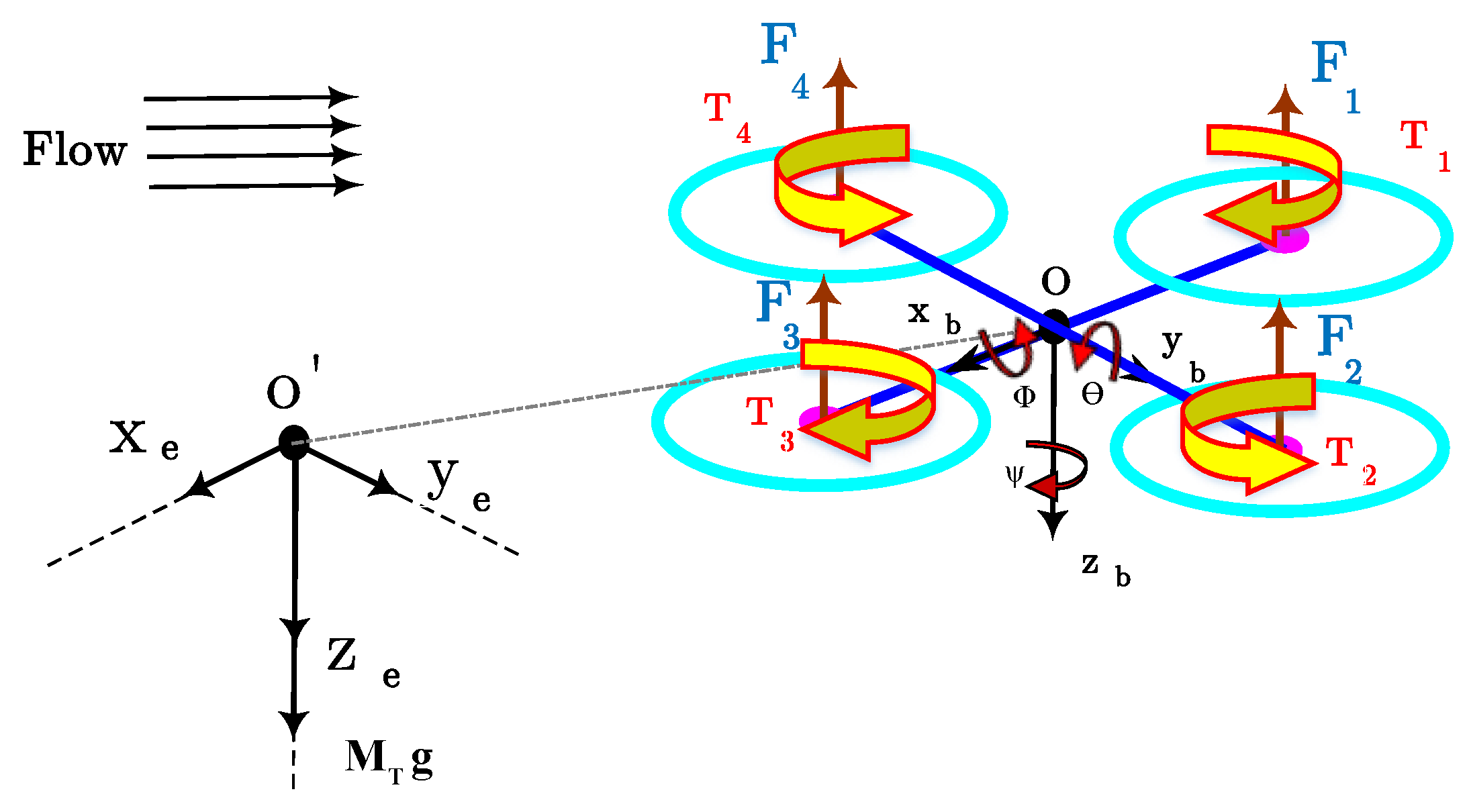
Figure 2.
Evolution of the B-spline.
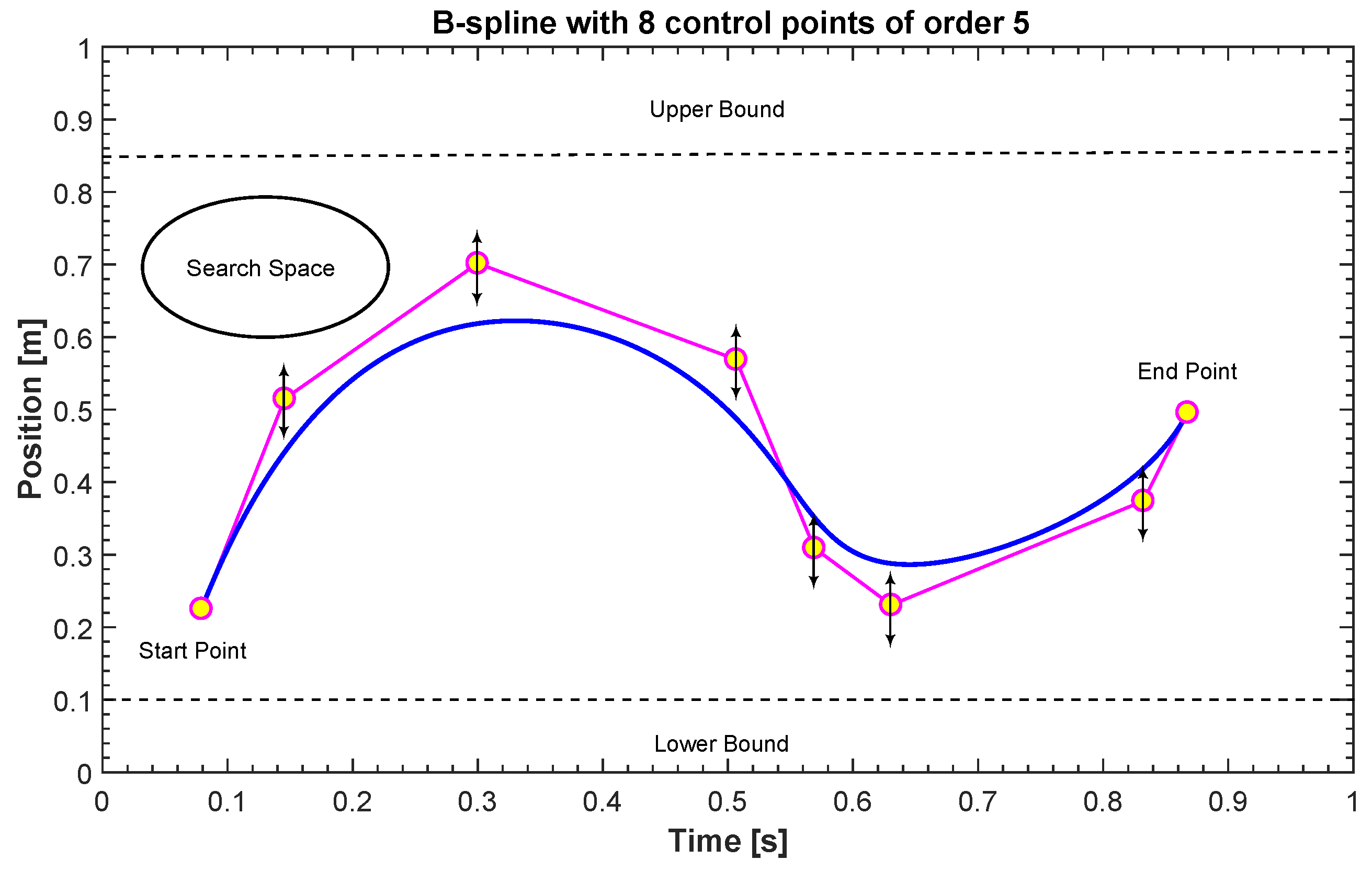
Figure 3.
Flowchart of trajectory generation algorithm. PSO: particle swarm optimization.
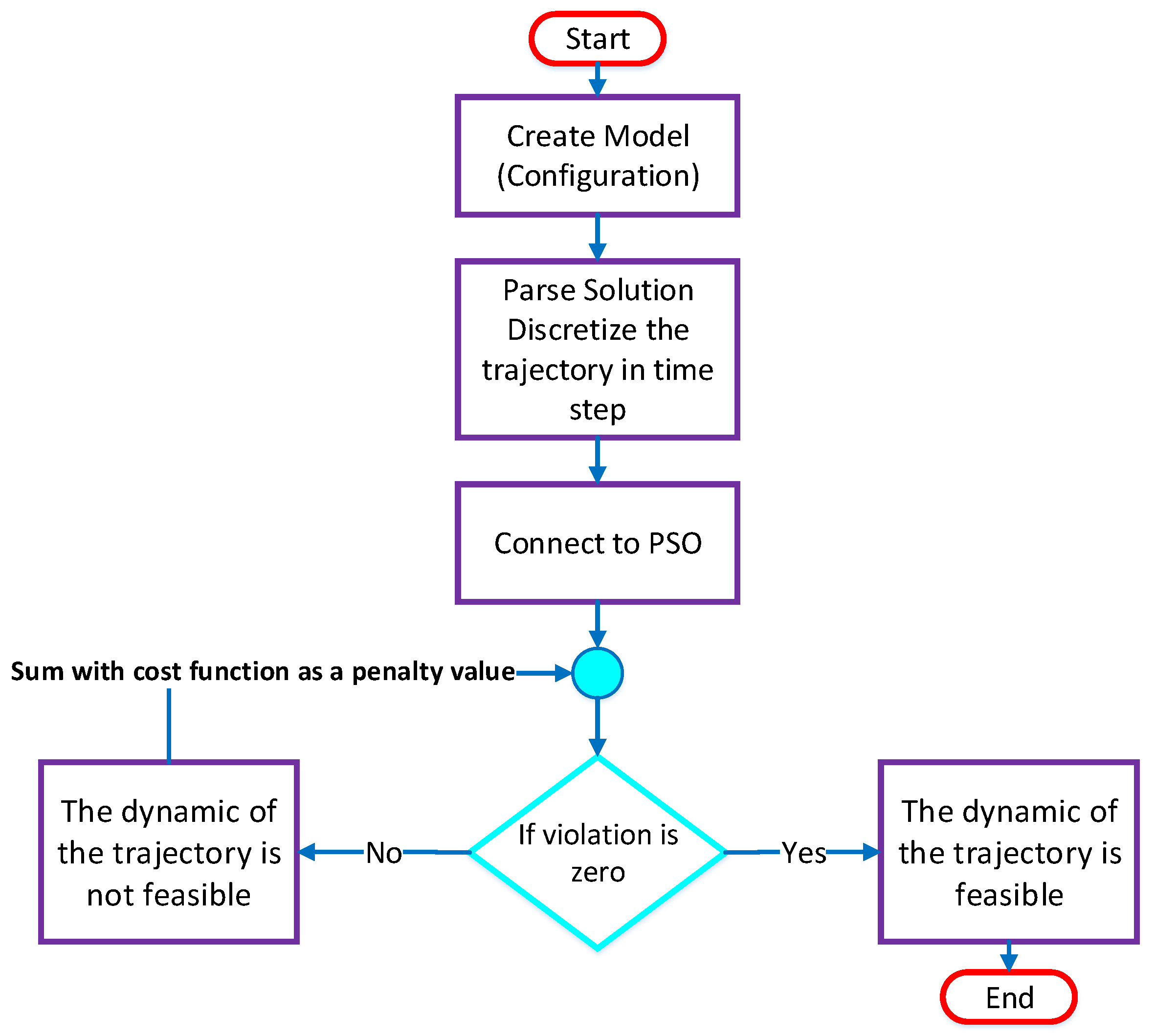
Figure 4.
Mathematical model of PSO.

Figure 5.
Stochastic realization for flight level (FL).

Figure 6.
Three-dimensional flight level (FL) trajectory.

Figure 7.
North east down (NED) for FL.

Figure 8.
Evolution of actuators torques for FL.

Figure 9.
Control efforts for FL.

Figure 10.
Translation of velocities and acceleration in FL.
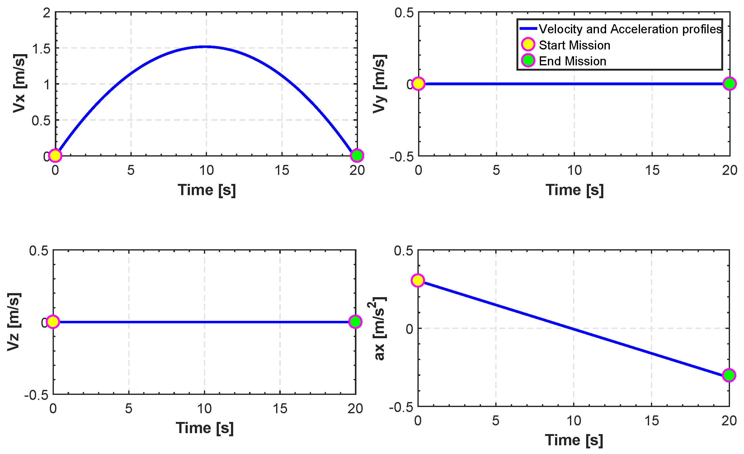
Figure 11.
Average cost function vs. iteration for FL.

Figure 12.
Three-dimensional take-off, mission and landing (TML) trajectory.
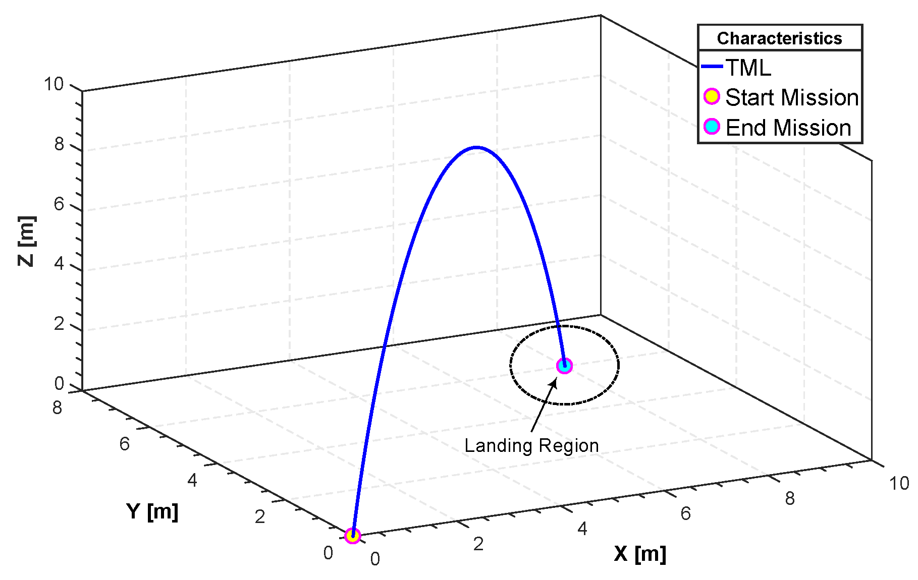
Figure 13.
Roll, pitch and yaw angle for TML.
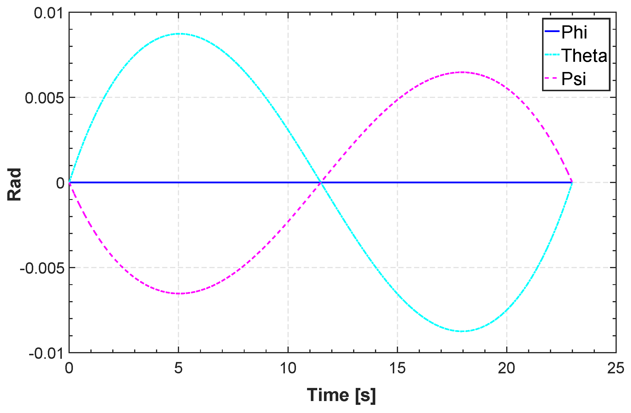
Figure 14.
North east down NED for TML.

Figure 15.
Translation of velocities and acceleration for TML.
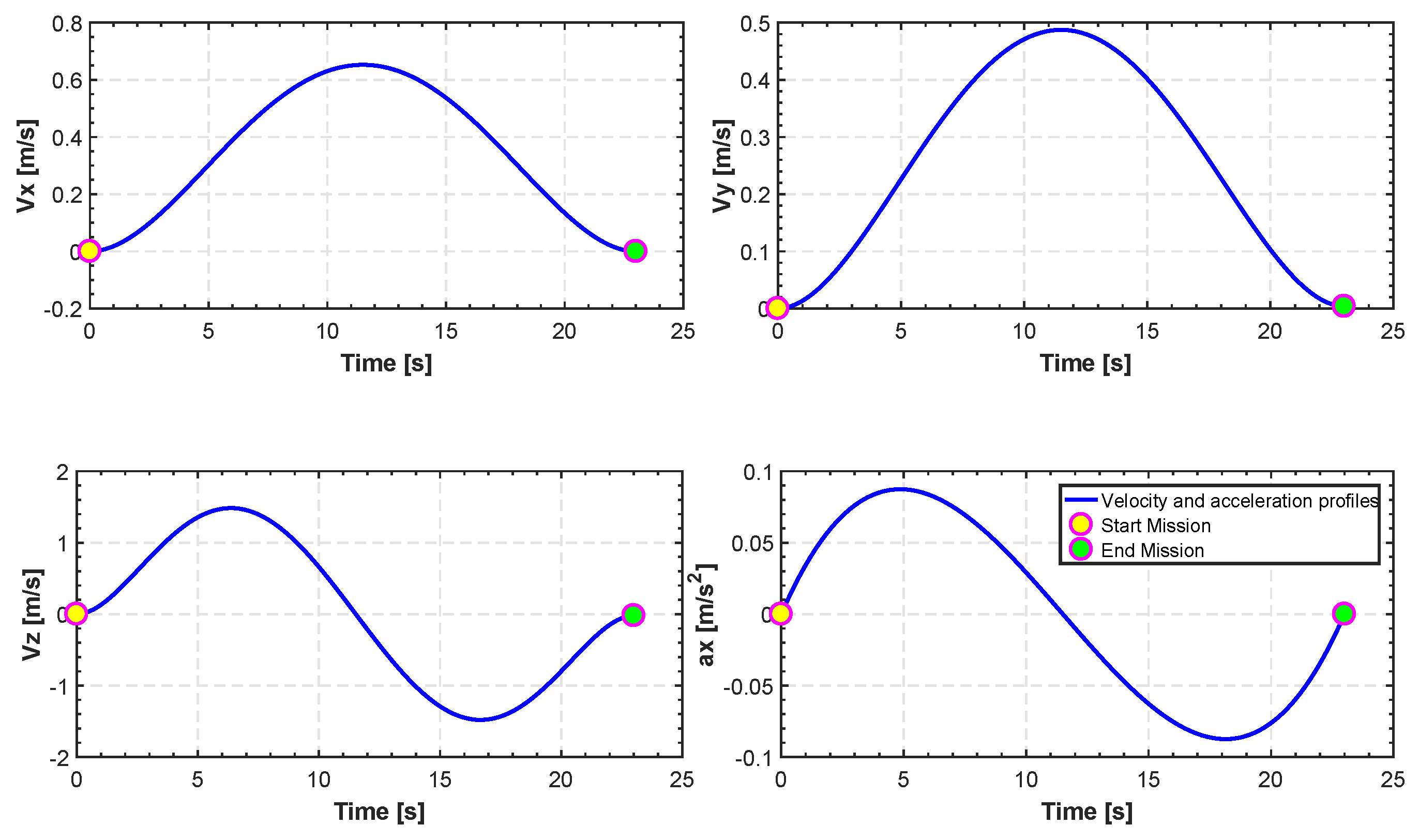
Figure 16.
Evolution of actuators torques for TML.
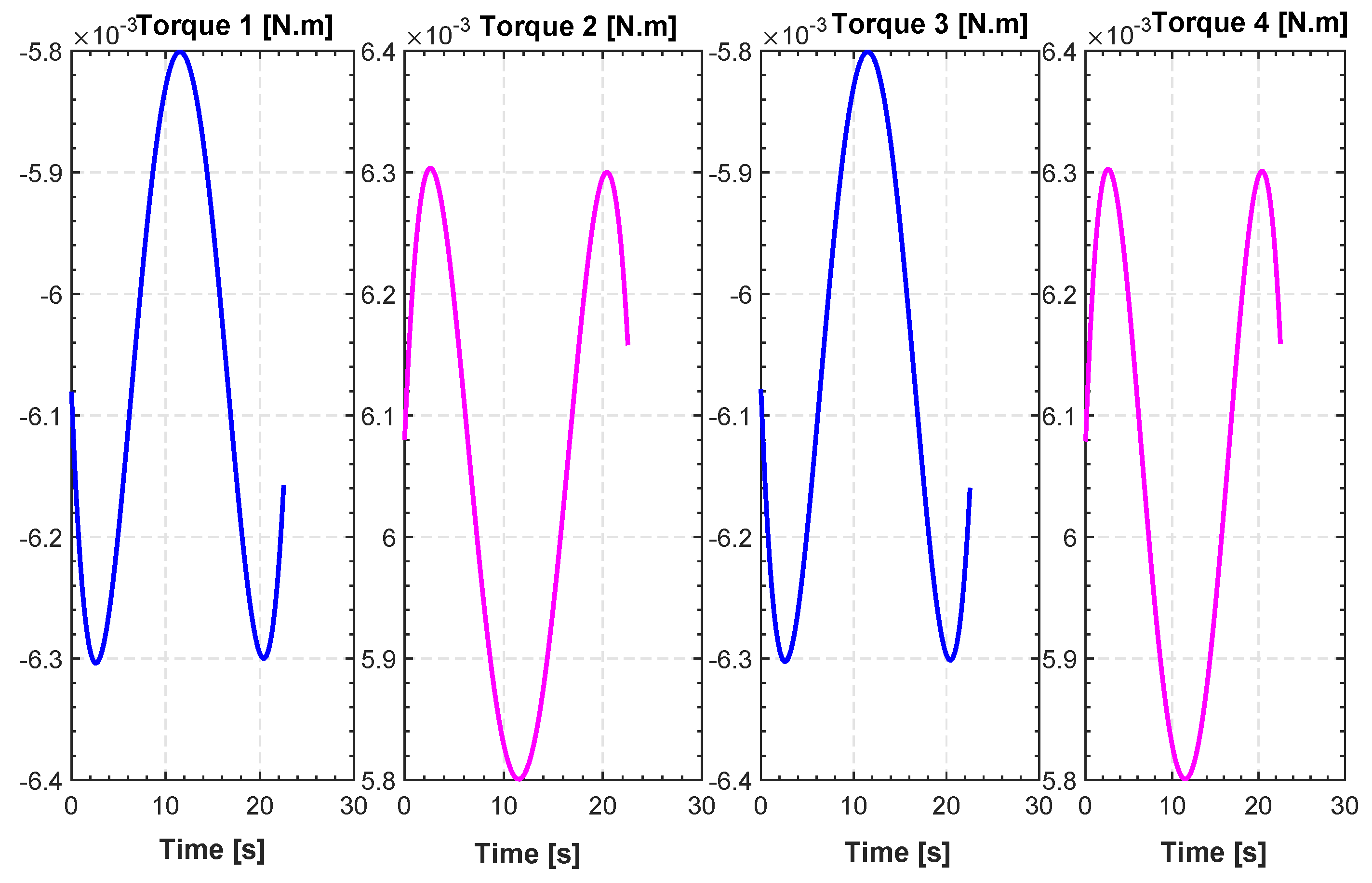
Figure 17.
Average cost function vs. iteration for TML.
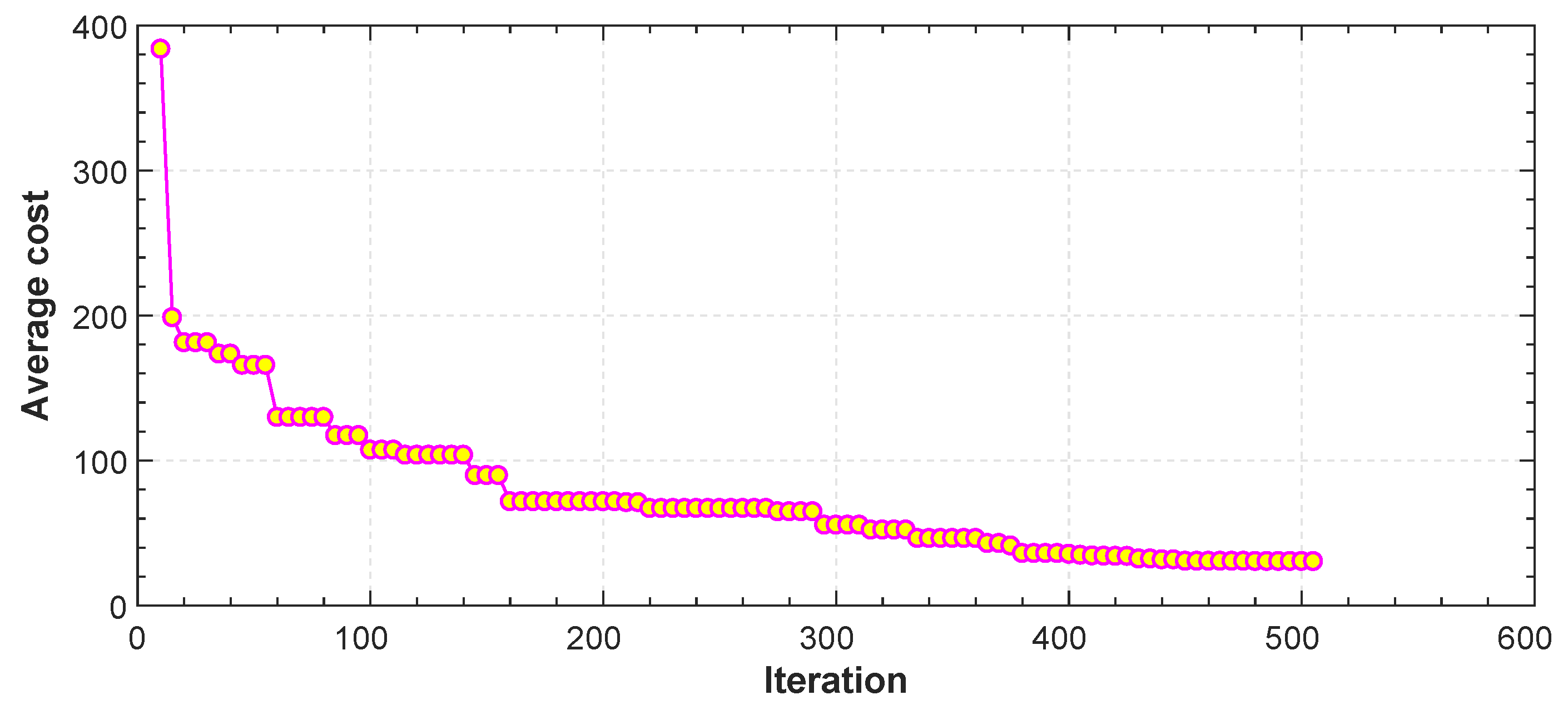
Figure 18.
Stochastic complex maneuvering in 3D space (CMS).

Figure 19.
Average cost function vs. iteration for CMS.
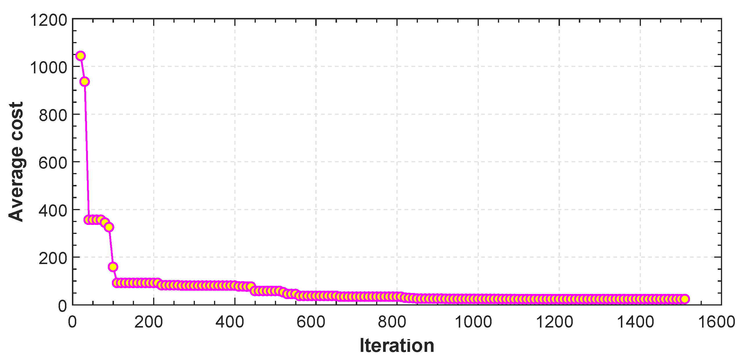
Figure 20.
Evolution of actuator torques for CMS.

Figure 21.
Complex maneuvering in 3D space (CMS).

Figure 22.
Roll, pitch and yaw angle for CMS.
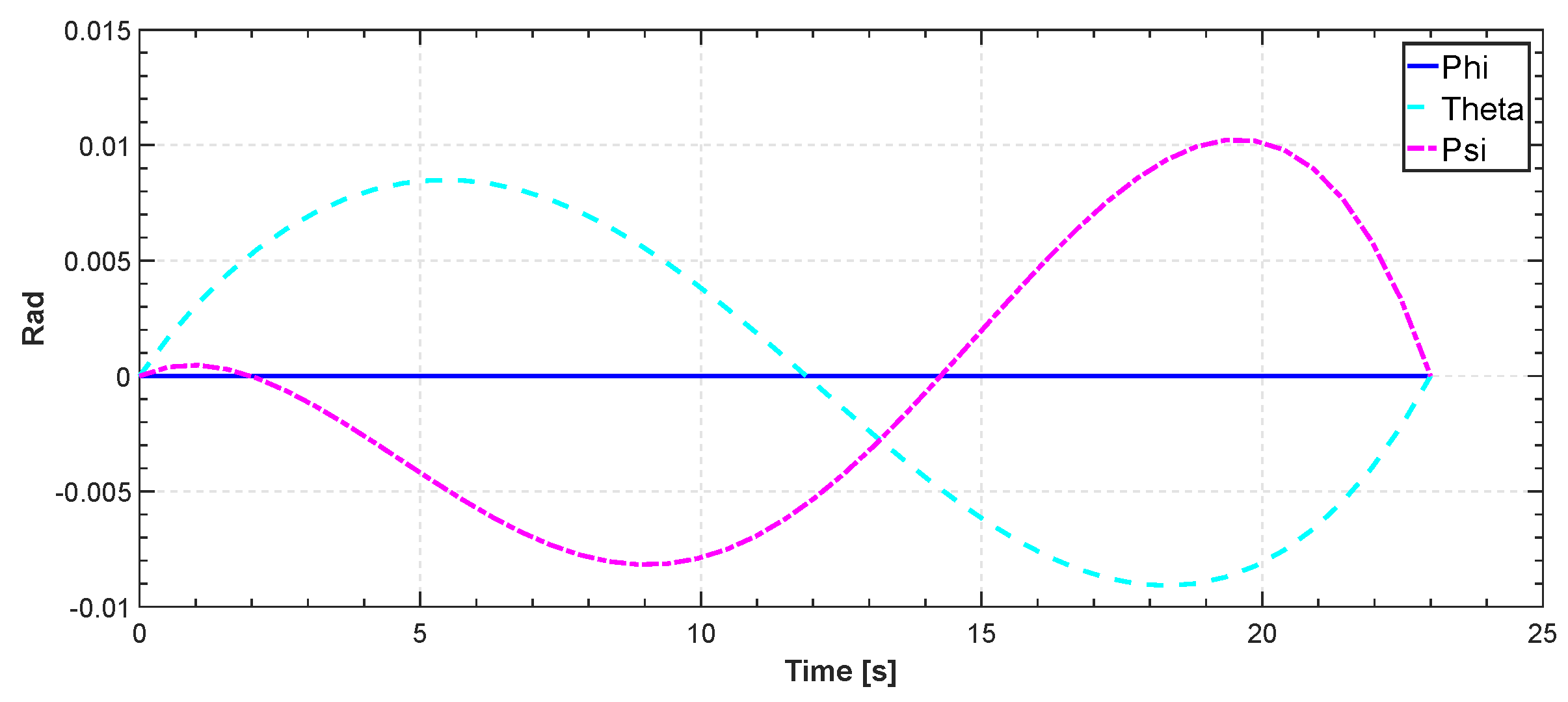
Figure 23.
Optimal path by rapidly-exploring random tree (RRT*), standard (A*) algorithm, genetic algorithm (GA) and the PSO.
Figure 23.
Optimal path by rapidly-exploring random tree (RRT*), standard (A*) algorithm, genetic algorithm (GA) and the PSO.


Table 1.
List of notations.
| Symbol | Definition |
|---|---|
| Earth axes | |
| NED | North east down |
| Body axes | |
| Roll angle | |
| Pitch angle | |
| Yaw angle | |
| Euler angles | |
| Rate of change of Euler angles | |
| Body angular rates | |
| Overall mass of the UAV | |
| Moment of inertia | |
| R | Radius of central sphere |
| g | Gravitational acceleration |
| Force generated by rotor | |
| Torque generated by rotor | |
| Angular velocity of rotor | |
| Control inputs |
Table 2.
Physical parameters of the quadrotor.
| Symbol | Unit |
|---|---|
| 0.65 Kg | |
| l | 0.232 m |
| g | 9.806 m/s |
| R | m |
| Kg m | |
| Kg m | |
| Kg m | |
| b | Ns |
| d | Nms |
| Nm | |
| 0.1 Rad | |
| 0.1 Rad | |
| 0.1 Rad | |
| Inertia Weight () | 1 |
| 2 | |
| 2 |
Table 3.
Solution details.
| Scenarios | Control Points | Swarm Size | Iterations | Execution Time |
|---|---|---|---|---|
| Scenario 1 | 4 | 50 | 250 | 5.090549 (s) |
| Scenario 2 | 5 | 100 | 400 | 6.572763 (s) |
| Scenario 3 | 5 | 100 | 450 | 7.464875 (s) |
Table 4.
Comparision Results.
| Parameters | RRT* | A* | GA | PSO + B-Spline |
|---|---|---|---|---|
| Length (m) | 18.1265 | 16.5563 | 17.2111 | 14.2095 |
| Execution time (s) | 17.343599 | 0.02315 | 9.230695 | 1.544244 |
© 2017 by the authors. Licensee MDPI, Basel, Switzerland. This article is an open access article distributed under the terms and conditions of the Creative Commons Attribution (CC BY) license (http://creativecommons.org/licenses/by/4.0/).
Share and Cite
MDPI and ACS Style
Salamat, B.; Tonello, A.M. Stochastic Trajectory Generation Using Particle Swarm Optimization for Quadrotor Unmanned Aerial Vehicles (UAVs). Aerospace 2017, 4, 27. https://doi.org/10.3390/aerospace4020027
AMA Style
Salamat B, Tonello AM. Stochastic Trajectory Generation Using Particle Swarm Optimization for Quadrotor Unmanned Aerial Vehicles (UAVs). Aerospace. 2017; 4(2):27. https://doi.org/10.3390/aerospace4020027
Chicago/Turabian StyleSalamat, Babak, and Andrea M. Tonello. 2017. "Stochastic Trajectory Generation Using Particle Swarm Optimization for Quadrotor Unmanned Aerial Vehicles (UAVs)" Aerospace 4, no. 2: 27. https://doi.org/10.3390/aerospace4020027
Note that from the first issue of 2016, this journal uses article numbers instead of page numbers. See further details here.