Effect of the Backward-Facing Step Location on the Aerodynamics of a Morphing Wing

Abstract

Over the last decade, aircraft morphing technology has drawn a lot of attention in the aerospace community, because it is likely to improve the aerodynamic performance and the versatility of aircraft at different flight regimes. With the fast paced advancements in this field, a parallel stream of research is studying different materials and designs to develop reliable morphing skins. A promising candidate for a viable morphing skin is the sliding skin, where two or more rigid surfaces remain in contact and slide against each other during morphing. The overlapping between each two panels create a backward-facing step on the airfoil surface which has a critical effect on the aerodynamics of the wing. This paper presents a numerical study of the effect of employing a backward-facing step on the suction side of a National Advisory Committee for Aeronautics (NACA) 2412 airfoil at a high Reynolds number of 5.9 × 10⁶. The effects of the step location on the lift coefficient, drag coefficient and critical angle of attack are studied to find a favorable location for the step along the chord-wise direction. Results showed that employing a step on the suction side of the NACA 2412 airfoil can adversely affect the aforementioned aerodynamic properties. A drop of 21.1% in value of the lift coefficient and an increase of 120.8% in the drag coefficient were observed in case of a step located at 25% of the chord length. However, these effects are mitigated by shifting the step location towards the trailing edge. Introducing a step on the airfoil caused the airfoil’s thickness to change, which in turn has affected the transition point of the viscous boundary layer from laminar to turbulent. The location of the step, prior or post the transition point, has a noteworthy effect on the pressure and shear stress distribution, and consequently on the values of the lift and drag coefficients.

1. Introduction

Nature has always been a source of inspiration for many engineering applications, and Aerospace engineering in particular is one the fields that holds a considerable share from these biomimetic inspired designs. Starting from the need of wings to fly, passing by the different airfoil designs and recently, the emerging need for morphing wings [1]. In the aeronautical field, morphing is a technology that increases the aircraft’s performance by manipulating its geometrical characteristics [2,3,4]. Morphing technology of wings can be divided into the following three categories; in-plane (span, sweep and chord), out-of-plane (twist, dihedral and bending) and airfoil (camber and thickness) morphing [5].

With the fast evolution of aircraft morphing technology, versatile morphing skins should be realized. Kikuta et al. [6] listed a number of mechanical and chemical properties, but the most demanding requirements is the combination between flexibility and a significant out-of-plane stiffness to bear all the aerodynamic loads. Among different designs of morphing skins, two groups of designs seemed to be promising, namely, stretching skin and sliding skin [7]. 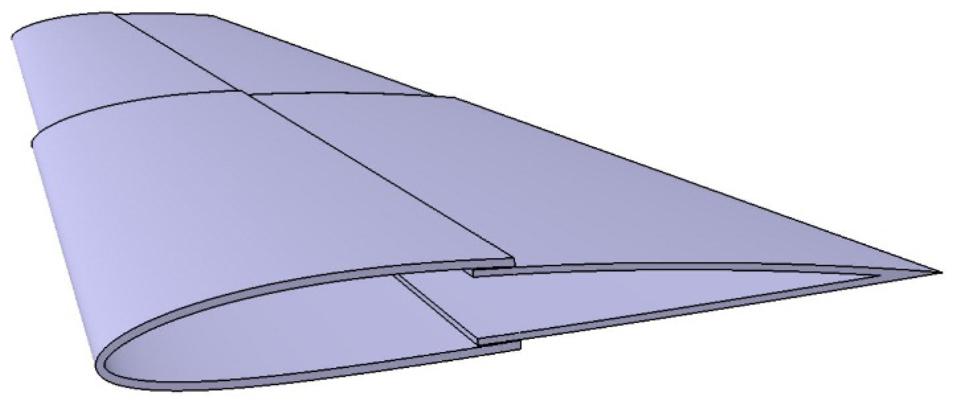Stretchable or flexible skin is popular among small-sized morphing aircraft as the Defense Advanced Research Projects Agency (DARPA) Smart Wing [8], where a high strain-to-failure silicone skin was tested. However, for the vast majority of air vehicles, the aerodynamic loads exceed the capabilities of stretchable skins, and the need of rigid surfaces is emphasized. On the other hand, sliding skins are rigid and provide a suitable surface to withstand the aerodynamic forces, particularly the pressure distribution. In these designs, rigid wing sections slide within an adjacent hollow wing. As such, two rigid surfaces remain in contact and slide against each other during morphing. From the aerodynamics perspective, the interface on wings with sliding skins is treated as backward-facing steps integrated on the wings’ surface as shown in Figure 1.

The telescopic design of the wing with steps along the chord-wise is imperative to allow the wing to morph in the required degrees of freedom.

While most of the current studies in this field focused on the mechanical design [9,10,11], the aerodynamic analysis of these models plays a vital role. Infinitesimal discontinuities on the morphing skin can drastically affect the overall aerodynamic performance, leading to the loss of all potential gains of the morphing wing.

This study focuses on the aerodynamics perspective of the employed backward-facing step of sliding morphing skins. As a first step in analyzing the complete aerodynamic performance of backward-facing steps, this paper examines a NACA 2412 (National Advisory Committee for Aeronautics) airfoil with a single step on the suction side. The effect of backward-facing step on the pressure side is currently being performed, and its implication is out of scope of the present paper.

The first time a similar concept was documented was in the early 1960s, when Richarde Kline and his colleague Floyd Fogleman designed a paper airplane that can fly longer distances despite wind and turbulence. The wings of their airplane were flat on top surface and partially hollowed at the bottom surface of the wing. In 1972, they filled a U.S. patent [12] for their wedged-like airfoil that is hollowed from below. Two years later, the National Aeronautics and Space Administration (NASA) sponsored an experimental study [13] to examine the Kline–Fogleman patented designs. The wind tunnel results showed that the lift-to-drag ratio of the new airfoil is lower than that of the flat plate and the pressure data showed that the airfoil derives its lift the same way as the inclined flat plate. The airfoil offered no advantages over the conventional airfoil. Despite these claims, the Kline–Fogleman airfoils inspired Fertis and Smith to design an airfoil with a backward facing step, this time on the suction side. They filled a U.S. patent [14] for their design titled “Airfoil”.

The experimental results of their designs were published six years later by Fertis [15]. Wind tunnel testing was performed on a NACA 23012 airfoil over a range of Reynolds numbers from 1 × 10⁵ to 5.5 × 10⁵, and a wide range of angle of attacks. Results showed improved stall characteristics at all tested airspeeds, increased lift coefficients and increased lift-to-drag ratios over a wide range of angles of attacks. This enhanced performance of airfoils with a backward facing step on the suction side was not in a perfect agreement with the results obtained by the numerical and experimental testing done by Finaish and Witherspoon [16]. In their study, they followed a more systematic way to examine 15 different configurations of a symmetric NACA 0012 airfoil. Backward-facing steps were located on either side of the airfoil, and the Reynolds number used in this study was 5 × 10⁵. Results showed that for most cases with the step installed on the upper surface, the lift-to-drag ratio decreased due to the increase in the drag, which was directly proportional to the step depth.

With most of the studies were performed at low Reynolds number, the current study offers a comprehensive and in-depth numerical analysis on the aerodynamic performance of a stepped NACA 2412 airfoil at a high Reynolds number. First, the numerical methods and the boundary conditions will be stated, followed by an assessment of the spatial convergence of the mesh. The numerical investigations will focus on three main aerodynamic properties, namely, the lift coefficient $c_l$, the drag coefficient $c_d$ and the critical angle of attack ${\alpha }_{cr}$. The effect of varying the step location will be thoroughly studied on the three aforementioned aerodynamic properties.

2. Numerical Modeling and Accuracy Assessment

2.1. Numerical Modeling

FLUENT is a general purpose commercial computational fluid dynamic (CFD) package that solves the Navier–Stokes equations using a finite volume method. In this study, the density-based solver implemented in FLUENT will be used to solve the governing continuity, momentum, energy and turbulence equations of the flow. The airfoil used is a NACA 2412 with a backward-facing step installed on the upper surface of the airfoil. The turbulence of the flow is modeled using the four equations Langtry–Menter transitional shear stress transport turbulence model (Transition-SST model) [17,18]. This turbulence model is based on coupling the SST $k-\omega$ transport equations with two other transport equations, one for the intermittency and one for the transition onset criteria in terms of momentum-thickness Reynolds number. Previous studies [18,19] showed that results of the transition-SST model fit well with the experimental results when compared to fully turbulence models such as the $k-\epsilon$ and the $k-\omega$ models. For that reason, this model was chosen to numerically model the turbulence of the flow over the airfoil.

2.2. Boundary Conditions and Baseline Parameters

The airfoil used in this study is a standard NACA 2412 (National Advisory Committee for Aeronautics) airfoil with a sharp trailing edge. This series of airfoils and its derivatives are commonly used for airplanes designed to operate at both subsonic and supersonic speeds, in addition to their applications in helicopter rotor blades and high performance propeller blades [20,21]. The chord length of the airfoil was set to unity, and its surface is treated as an adiabatic no-slip wall. The air around the airfoil is modeled as an ideal gas whose reference temperature is set to 300 K. A C-mesh topology was created around the airfoil with an extended far-field boundary that is 32 chords away from the airfoil. The far-field boundary conditions are set to pressure far-field with 0.16174 Mach number and a Reynolds number of 5.9 × 10⁶. The angle of attack of the flow was set to 2.5°, unless otherwise stated.

Second order convergence schemes were used in calculating the convective and diffusive fluxes of the discretized transport equations, and a least squares cell based method was used to reconstruct the gradients of the scalar quantities.

The baseline design is a NACA 2412 airfoil with a vertically oriented step installed on the upper surface. To choose the step depth, seven different step sizes have been tested ranging from 0.0075 of the chord length to 0.025 of the chord length. The seven configurations obtained similar correlation between the flow properties (lift coefficient, drag coefficient and the critical angle of attack) and the step location. For that reason, the step depth that is presented in this study is the mid value of 0.015 chords. After the step, the airfoil curvature follows original NACA 2412 profile, but scaled along the Y-direction to create the required descent that matches the step depth. Figure 2 shows a schematic diagram of a clean NACA 2412 overlaying an airfoil with a step located at a distance $X_U$ from the leading edge.

2.3. Examining the Spatial Convergence

Choosing the optimal density of the mesh to discretize the computational domain is an essential and challenging task in computational fluid dynamics. The mesh has to be fine enough to capture the required details of the flow, and to be computationally affordable in terms of the computational power. To reach this demanding balance, the Richardson’s extrapolation method is used on a family of three consecutively refined meshes as proposed by John C. Vassberg and Antony Jameson [21].

This approach provides an estimation of the order of convergence $p$ of the numerical solution by tracking an aerodynamic property $ℱ$ on a family of three consecutively refined meshes. The property $ℱ$ is evaluated on the coarse, medium and fine meshes to obtain ${ℱ}_c$, ${ℱ}_m$ and ${ℱ}_f$ respectively. The subscripts c, m and f stands for “coarse”, “medium” and “fine” respectively. These values are extrapolated using Richardson’s extrapolation method to calculate the continuum value ${ℱ}_{h=0}$. This value represents the expected value when the spacing between the nodes of the mesh tends to zero. The continuum value ${ℱ}_{h=0}$ is calculated from the three values ${ℱ}_c$, ${ℱ}_m$ and ${ℱ}_f$ as follows:

$${ℱ}_{h=0}\cong {ℱ}_f+\frac{{ℱ}_f-{ℱ}_m}{r^p-1}$$

(1)

where $r$ is the refinement ratio, and in our case it is constant at 2. While $p$ is the observed order of accuracy of the solution and is calculated as:

$$p=\frac{ln\left(\frac{{ℱ}_c-{ℱ}_m}{{ℱ}_m-{ℱ}_f}\right)}{ln\left(r\right)}$$

(2)

This order of accuracy could be also calculated from the logarithmic slope of the errors of the three meshes ${\epsilon }_c$, ${\epsilon }_m$ and ${\epsilon }_f$. In this case, the error of $ℱ$ in each mesh is calculated as:

$${\epsilon }_c=|{ℱ}_{h=0}-{ℱ}_c|, {\epsilon }_m=|{ℱ}_{h=0}-{ℱ}_m| \text{and} {\epsilon }_f=|{ℱ}_{h=0}-{ℱ}_f|$$

(3)

This methodology is used on the three consecutively refined meshes shown in Figure 3.

The number of quadrilateral cells in each mesh is approximately 12,000 for the coarse mesh, 48,000 for the medium mesh and 192,000 elements for the fine mesh. The aerodynamic property $ℱ$ is chosen to be the lift coefficient $c_l$. The convergence of the solution is judged by the complete stability of the lift, drag and moment coefficients. Equations (1)–(3) were used to assess the spatial convergence of the grids used. The order of accuracy of the solution could be calculated using Equation (2) and is shown as the slope of the red line in Figure 4a.

The computed order of accuracy $p$ was found to be 2.03 which is in a very good agreement with the second order discretization schemes used. Figure 4a shows that the line joining ${\epsilon }_c$, ${\epsilon }_m$ and ${\epsilon }_f$ is perfectly parallel to the second order slope line. Figure 4b shows that the value of the lift coefficient obtained from the fine mesh is 0.244% away from the asymptotic value ${ℱ}_{h=0}$. This means that the results obtained from the fine mesh is very close to the asymptotic continuum value ${ℱ}_{h=0}$, and further refinements will be perceived as additional computational expenses with negligible improvement in the calculated numerical values. Thus, the fine mesh will be used in this study to examine the aerodynamic performance of the stepped NACA 2412 airfoil.

3. Results and Discussion

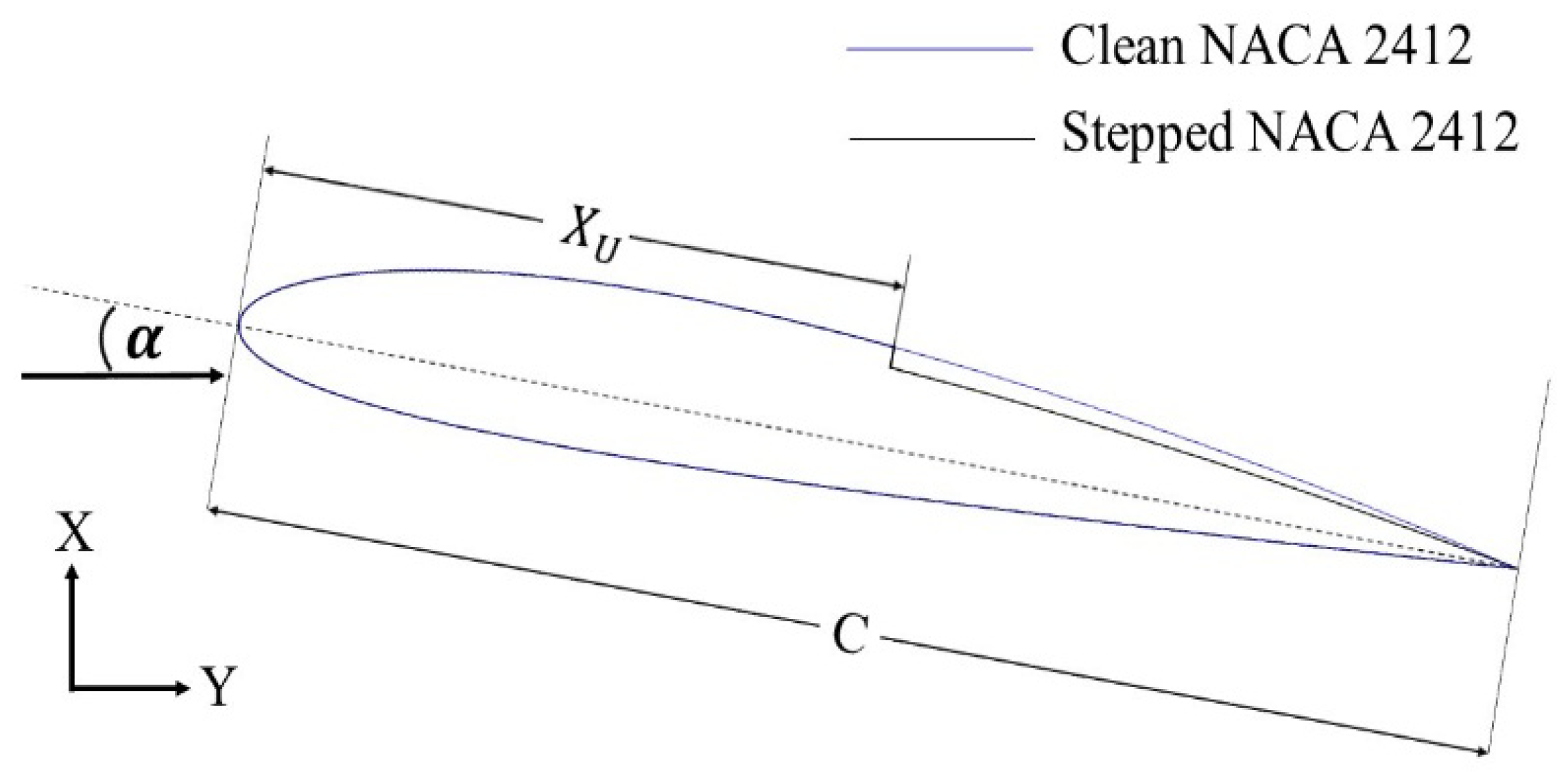
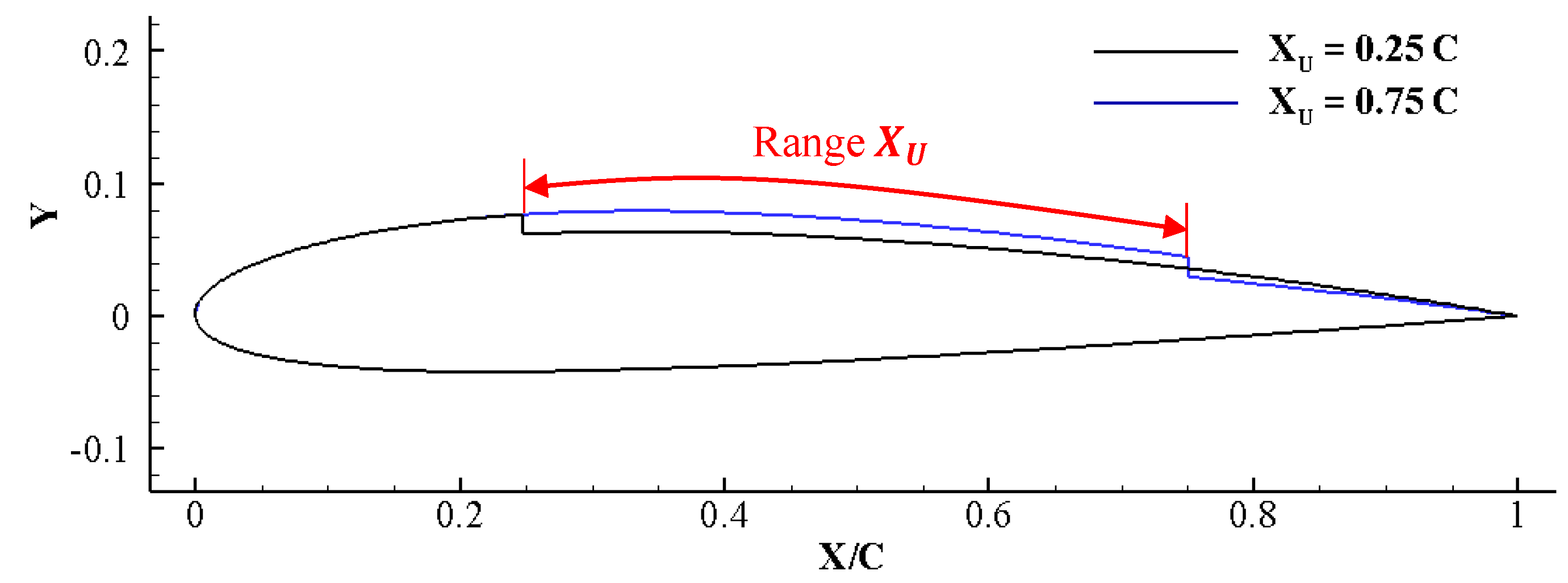
In this section the effect of the step location on the aerodynamics of the stepped NACA 2412 airfoil will be examined. The location of the step changed from 25% to 75% along the unity chord length of the airfoil, with an increments of 5% from one configuration to the other. Figure 5 shows the two extreme positions of the step at $X_U=0.25 C$ and $0.75 C$, respectively.

In each simulation, the lift, drag and moment coefficients were monitored until completely steady values were reached.

3.1. Effect of the Step Location on the Lift Coefficient c_l

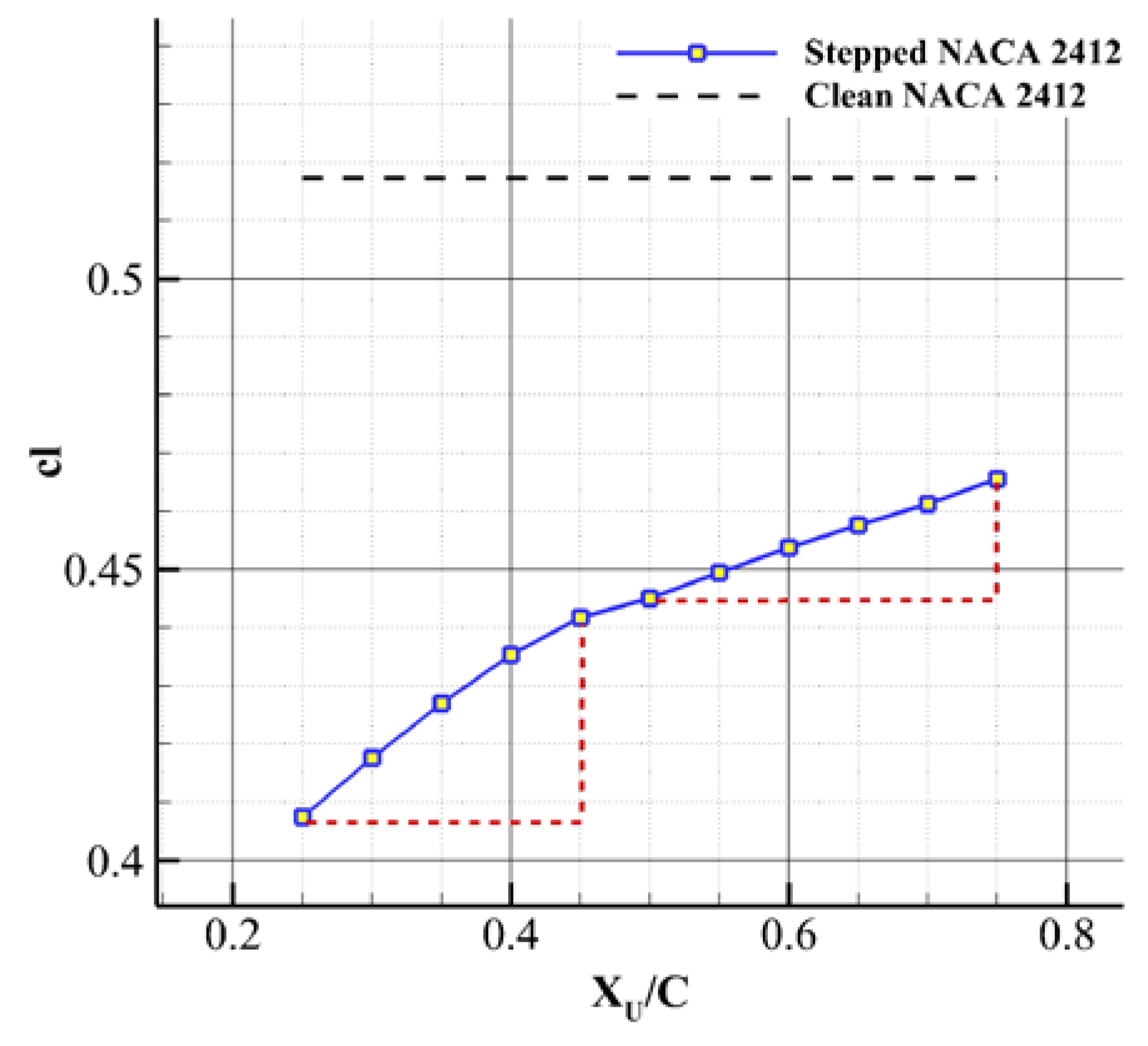
The variation of the lift coefficient $c_l$ with the step locations was calculated and plotted as shown in Figure 6. Two main properties are observed in the trend of the curve shown. The first observation is the direct relationship between the step location $X_U$ and its corresponding lifting force. As the step is shifted along the chord-wise direction, the value of the lift coefficient increases. The second observation is the sudden change in the slope of the points located before $X_U/C=0.4$ and the points after $X_U/C=0.5$. The justification of these two observations can only be reached by an in-depth analysis of the flow properties around the stepped airfoil.

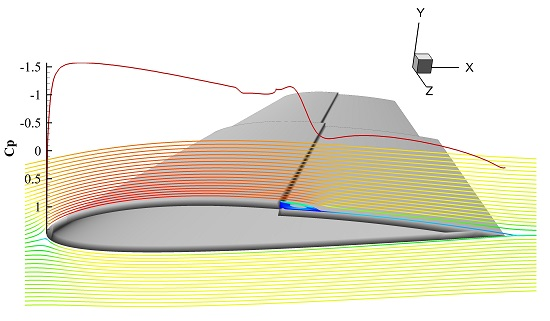
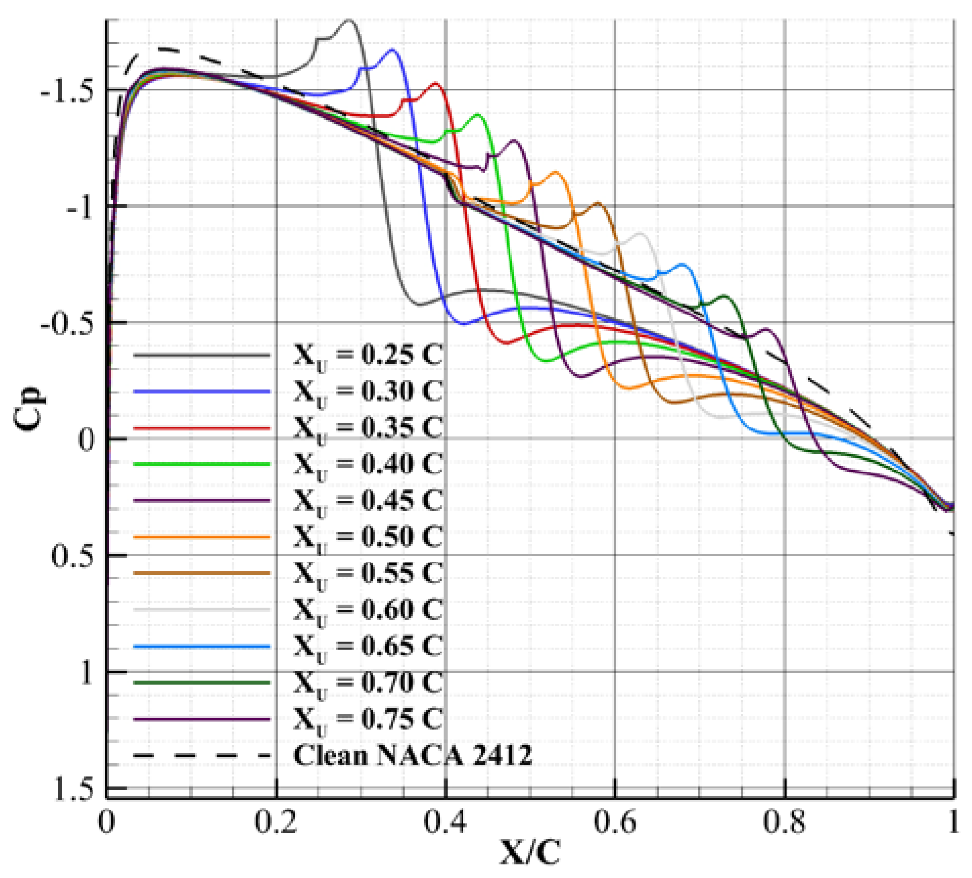
The fundamentals of airfoil aerodynamics indicate that the lifting force is mainly influenced by the pressure distribution around the airfoil. Therefore, to investigate the direct relation between the step location and the lift coefficient $c_l$, the distribution of the pressure coefficient $C_p$ over the stepped airfoil is plotted in Figure 7 for the different step locations, as well as the pressure distribution over a clean NACA 2412 airfoil.

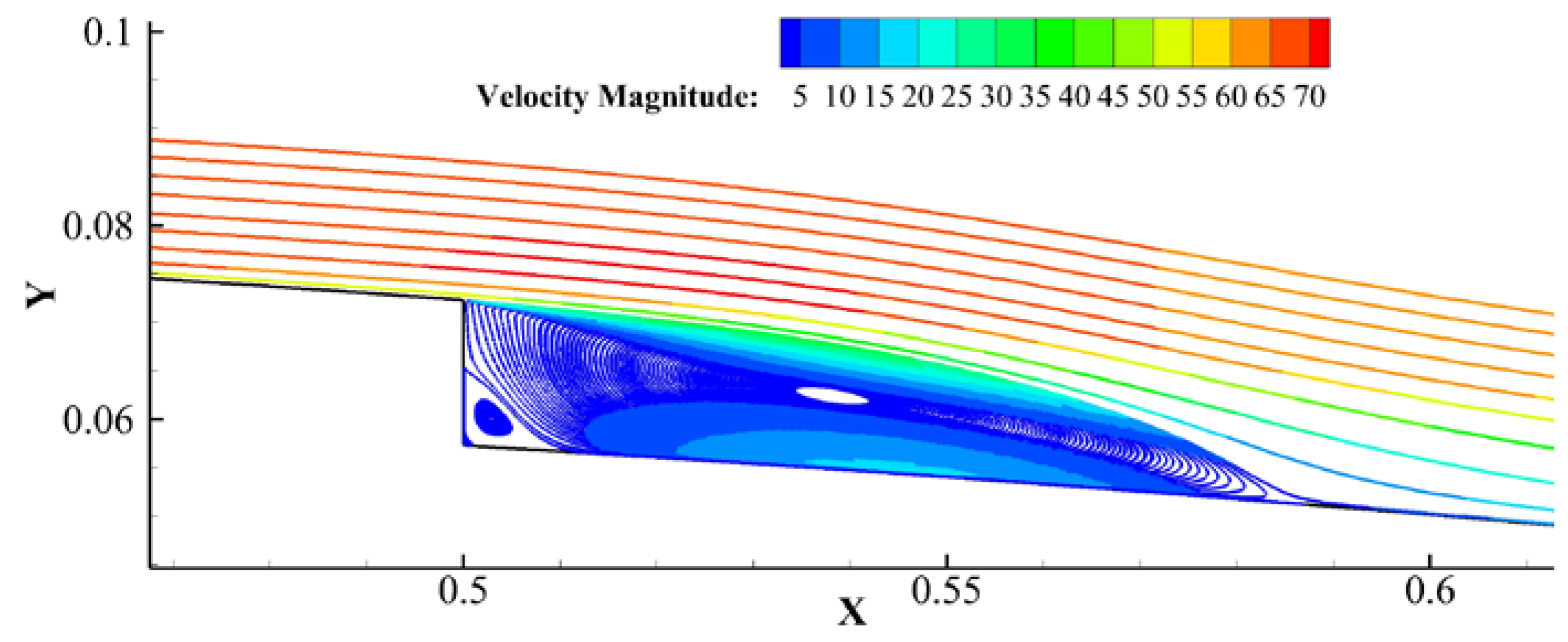
The pressure field experiences the normal drop at the leading edge due to the acceleration of the fluid over the airfoil’s curvature. When the flow travels past the backward-facing step, it creates a low pressure recirculation zone that increases the lifting force. However, the sudden reduction in the airfoil thickness after the step relatively decreases the flow velocity which results in a subsequent high pressure region stretched to the trailing edge of the airfoil. Figure 8 shows the separation of the flow and its subsequent reattachment at the end of the recirculation zone. Note also the presence of three different length scales of vortices trapped at the corner of the step. Theoretically, an infinite sequence of closed eddies with decreasing size and strength is expected.

The increase of the pressure over the suction side of the airfoil significantly affects the value of the lift coefficient and drops it below the value obtained from the clean NACA 2412 airfoil. At the same boundary conditions, a clean NACA 2412 obtains a lift coefficient value of 0.5172 which exceeds all the values observed in Figure 6. As the step location shifts towards the trailing edge, the region of high pressure diminishes, and the lift coefficient increases. This justifies the direct relationship between the step location and the value of lift coefficient $c_l$.

The second observation in Figure 6 is the change of the slope for the points located before $X_U/C=0.4$ and the points after $X_U/C=0.5$. This change in the slope is mainly driven by relative position of the step with respect to the point at which the laminar boundary layer experiences a transition from laminar to turbulent. With the boundary conditions stated in Section 2.2, the transition point is approximately at $X/C=0.425$ for cases of stepped airfoil and at $X/C=0.41$ for the clean airfoil at the same conditions. For cases where the step is located before $X/C=0.425$, the presence of the step triggers the transition before the point where it naturally occurs on the clean airfoil. For the other cases where the step is after the natural transition point, the step has an effect on the transition phenomena, prolonging the instability of the boundary layer. This difference in behavior is the main reason for the change in the slope.

Notes about the Viscous Boundary Layer Transition and the Numerical Modeling

The viscous boundary layer transition is observed in Figure 7 as a noticeable increase in the pressure approximately at $X/C=0.425$. This change in the pressure distribution is not observed in cases of airfoils with step before $X_U/C=0.4$, because in these cases the location of the step interrupt the stability of the boundary layer and triggers an early transition from laminar to turbulent.

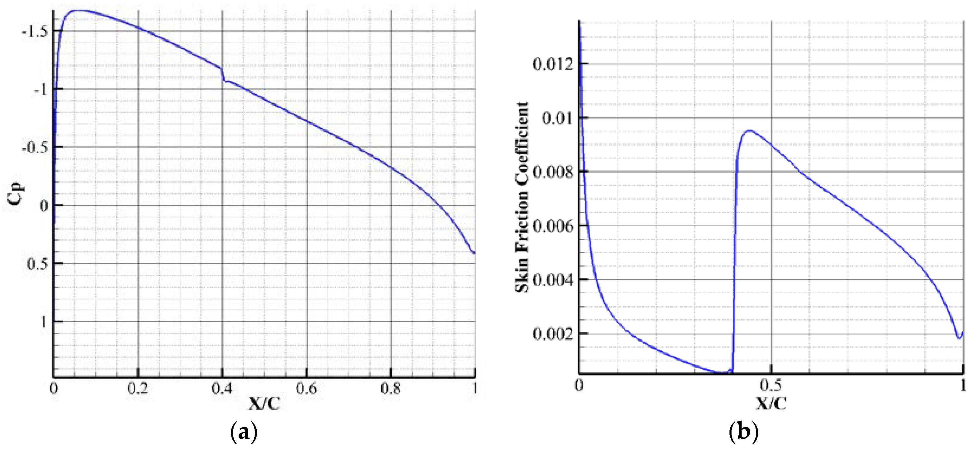
A similar but an amplified increase is noticed in the value of the skin friction coefficient at the same location. These sudden changes in the values of the pressure distribution and the skin friction coefficient are also observed in case of a clean NACA 2412 airfoil but slightly earlier at $X/C=0.41$ as shown in Figure 9a,b.

These abrupt changes in the pressure and skin friction coefficient values were not observed when a fully turbulent model as the $k-\epsilon$ or the $k-\omega$ models were used. Langtry and Menter [18] observed the same sudden change in the value of the skin friction coefficient over Aerospatiale A and the McDonald Douglas 30P-30N airfoils when the flow was modeled using the transition-SST turbulence model. This jump in the values of the skin friction coefficient fits well with the experimental results shown in their study, while the fully turbulent models showed discrepancies at these locations. 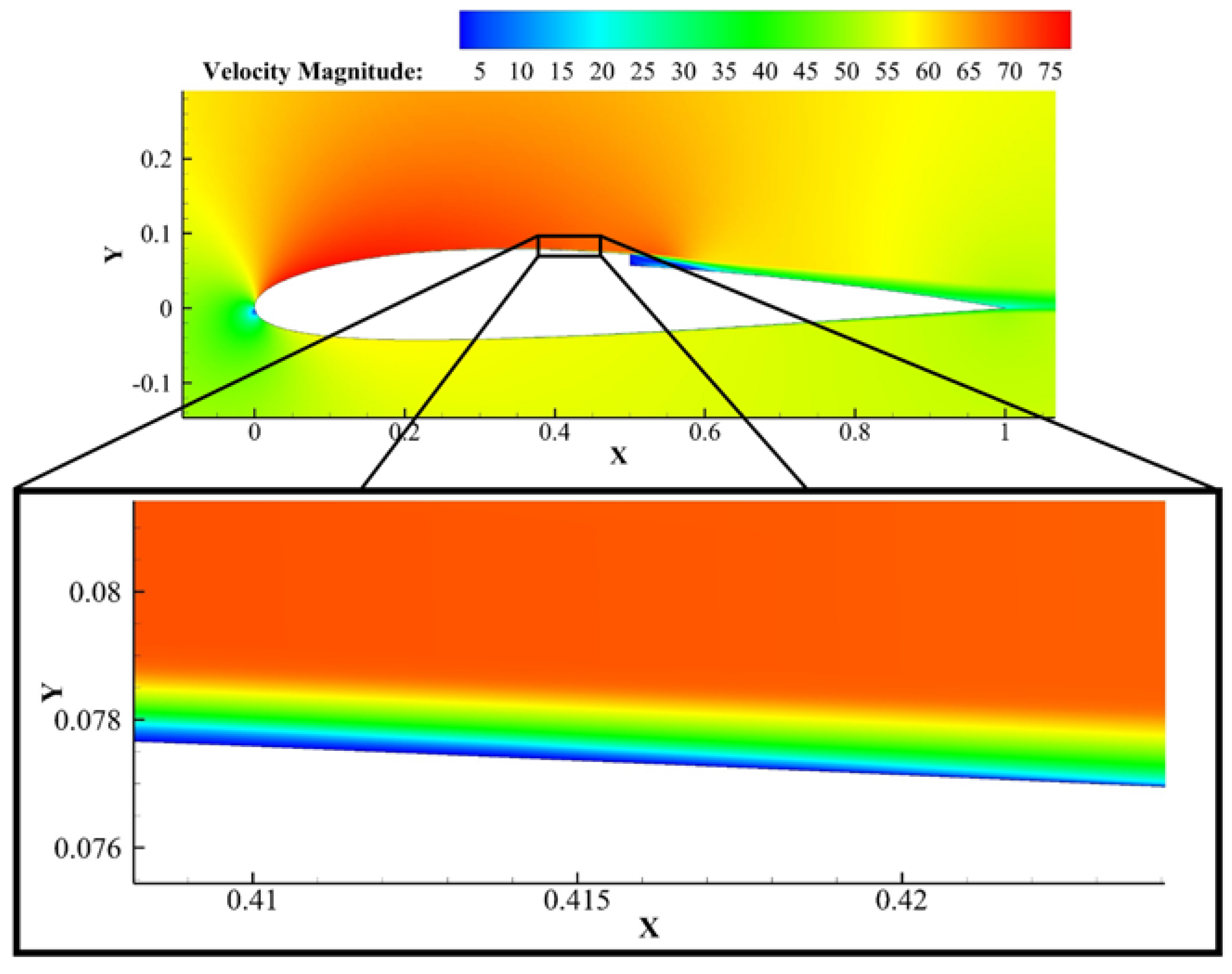Figure 10 shows a velocity contour plot with a close-up on the transition point. The numerical model clearly captured the transition of the laminar boundary layer to a turbulent boundary layer overlaying a laminar sublayer at approximately $X/C=0.425$.

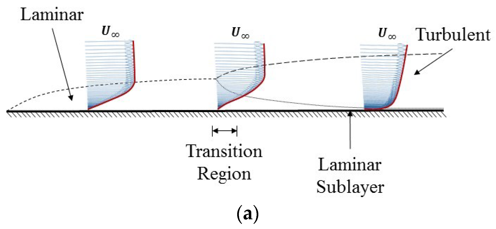
At the leading edge of airfoils (or any surface in general), the viscous boundary layer is laminar in nature, with a smooth and gradual gradient in the velocity of the flow layers adjacent to the airfoil. The velocity vectors will follow a monotonic curvature as shown in Figure 11a. Somewhere between 0.35 and 0.7 of the chord length, this laminar boundary layer starts a transition phase from laminar to turbulent. The exact location of this transition is controlled by a number of factors including curvature of the airfoil, turbulent intensity of the flow, Mach number, Reynolds number, angle of attack, etc. At this transition region, the viscous boundary layer is transversely bifurcated into two branches; a thin laminar sublayer attached to the airfoil surface, above which, a turbulent layer exists. At the transition region, the velocity vectors will follow an S-shaped curve as shown in Figure 11a. After transition from laminar to turbulent, the boundary layer can be divided into four main regimes. The first regime is at the airfoil surface which has a zero velocity due to the no-slip condition of the flow. Just above the surface, a thin laminar layer called the viscous sublayer or the laminar sublayer exists. At this layer, the flow velocity is linear with the off-wall distance. The viscous sublayer is followed by another thin region called the buffer layer, and that is where the flow begins the transition from laminar to turbulent. The last layer is the turbulent layer, at which the flow velocity is related to the log of the off-wall distance. The above described transition from laminar to turbulent was accurately captured in the numerical simulations of the flow. 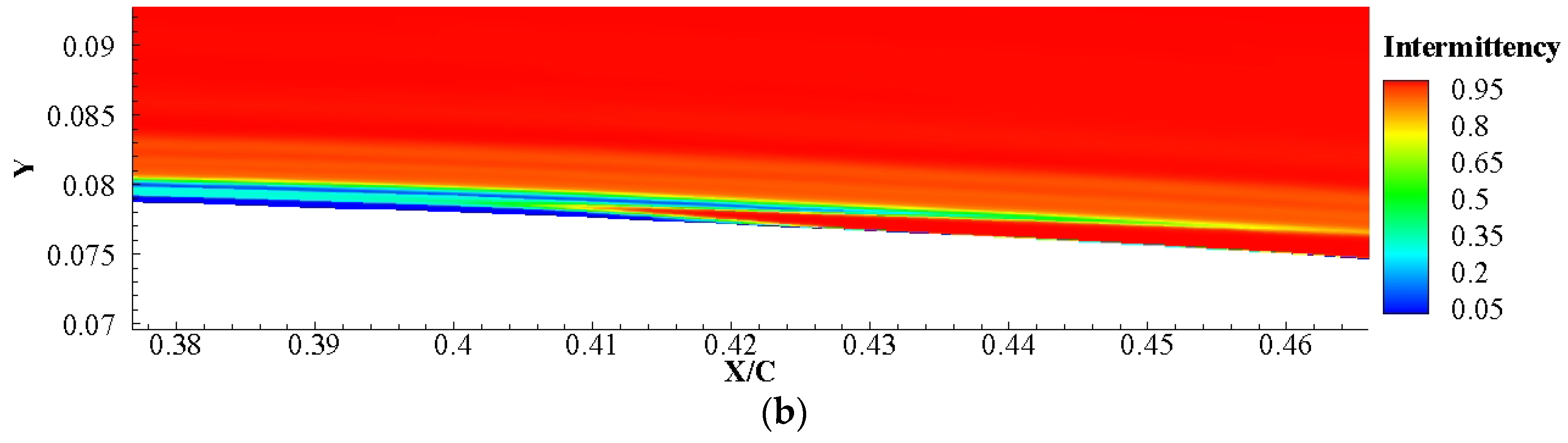Figure 11 shows a comparison between schematic diagram of the transition of the viscous boundary layer, and the intermittency contour plot of a stepped airfoil at the transition region.

Intermittency is usually a measure of the irregular alternation of phases. In the SST-Transitional turbulence model, the value of intermittency can distinguish between laminar regimes and turbulent ones. When the intermittency value is 0, the SST turbulence model is suppressed and the flow is treated as a laminar flow, while at a maximum value of 1 the SST model is active and the flow is fully turbulent. Thus, a contour plot of the intermittency can numerically capture the transition of the viscous boundary layer from laminar to turbulent. Figure 11b shows that the contour plot of the intermittency successfully modeled the bifurcation of viscous boundary layer to laminar sublayer and turbulent layer as compared to the schematic diagram shown in Figure 11a.

3.2. Effect of the Step Location on the Drag Coefficient c_d

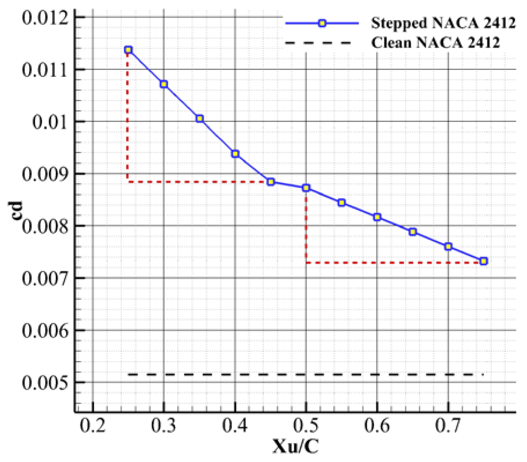
The drag coefficient of each case was calculated as the location of the step slid from the leading edge towards the trailing edge. The relation between drag coefficient and the location of the step is shown in Figure 12.

Similar to the observations in Figure 6 and Figure 12 reflects two main characteristics of the relation between the drag coefficient $c_d$ and the step location. The first observation is the inverse relation between the drag coefficient values and the step location. The drag coefficient decreases with the increase of the step distance from the leading edge, and continuously approaches the value of the clean airfoil. The second observation is again related to the sudden change in the slope of the lines before and after the location of transition of the viscous boundary layer, which is approximately at $X/C=0.425$.

These two observations could be understood by decomposing the drag coefficient into its main components, namely, the pressure drag and the skin friction drag coefficients as shown in Equation (4):

$$c_d=c_p+c_f=\frac{1}{\rho v^{2}A} {\int }_S\left(p-p_0\right)\left(\widehat{n} . \widehat{i}\right)dA+\frac{1}{\rho v^{2}A} {\int }_S{\tau }_w\left(\widehat{t} . \widehat{i}\right)dA$$

(4)

where $c_p$ is the pressure drag coefficient, $c_f$ is the friction drag coefficient or viscous drag coefficient, $\rho$ is the fluid density, $v$ is the reference velocity, $A$ is the reference area, $p$ is the pressure at the surface $dA$, $p_0$ is the reference pressure, $\widehat{n}$ is a unit vector normal to the surface $dA$, ${\tau }_w$ is the wall shear stresses at the surface $dA$ and $\widehat{t}$ is a unit vector tangent to the surface $dA$. Usually for streamlined bodies (as airfoils at small angles of attack), the value of the pressure drag coefficient is small compared to the viscous drag coefficient. This makes the graphs of wall shear stresses ${\tau }_w$ or the skin friction coefficient good tools to compare the drag forces on different airfoils designs. Equation (4) shows that as the area under the curves of the skin friction coefficient increases, the viscous forces and consequently the drag forces increase. Therefore, to justify the relation between the drag coefficient and the step location in Figure 12, the skin friction coefficient values of the NACA 2412 airfoil are plotted in Figure 13.

Figure 13 is divided into two subplots because of the different nature of the skin friction coefficient values for cases with a step located before the transition point ($X/C=0.425$) and after this point. In Figure 13a where the step is located before the transition point, the skin friction coefficient drops smoothly reflecting the laminar behavior of the viscous boundary layer, but the presence of the step interrupts this laminar behavior and triggers the transition of the viscous boundary layer from laminar to turbulent. The skin friction coefficient value drops to zero after the step due to the presence of a cascade of small sized and low energy eddies trapped at the corner of the step. This is followed by a concaved down curve confining the recirculation zone. After the reattachment of the boundary layer at the end of the recirculation zone, the skin friction coefficient will follow the natural pattern for an airfoil but with a longer turbulent region than the clean airfoil has. On the other hand, the curves in Figure 13b show that the presence of the step after the natural transition point has an important influence on the behavior of the skin friction coefficient. It prolonged the transition region and minimized the turbulent one before dropping towards zero at the tip of the airfoil.

As the step is shifted towards the trailing edge, the area under the curves in Figure 13b increases, and the drag coefficient should have increased, but this contradicts the values shown in Figure 12, where the drag coefficient values followed a negative slope when plotted versus the step location. This means that the pressure drag may be the dominant component in the drag coefficient value in cases of airfoils with a backward facing step, and only a decomposition of the drag coefficient can resolve this contradiction.

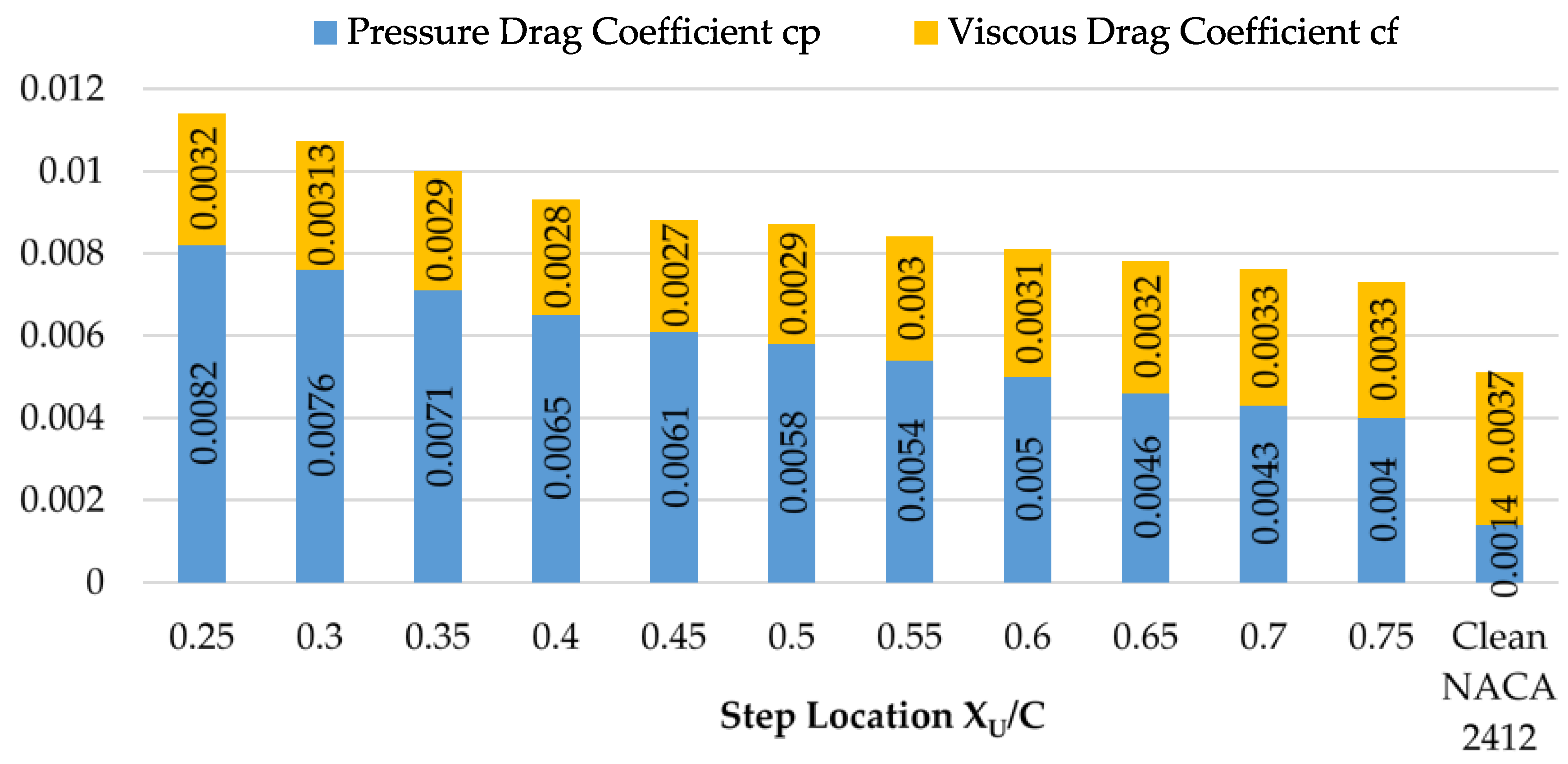
Equation (4) is used to decompose the value of the drag coefficient to its main components $c_p$ and $c_f$. Figure 14 shows the decomposed values of the drag coefficient in case of a clean NACA 2412 airfoil and in cases when the step is employed at different locations on the upper surface of the airfoil.

In all cases, the value of the viscous drag coefficient is nearly constant, and the variation of the pressure drag coefficient controls the variation of the overall drag force. This domination of the pressure drag coefficient is due to the separation of the flow at the step edge, leading to the formation of a low pressure recirculation zone acting on the vertical wall of the step. This creates an adverse force on the airfoil that significantly increases the pressure drag. For that reason, it is insufficient to use the skin friction coefficient values as a sole assessment of the variation of the drag coefficient. The pressure distribution over the airfoil will provide a better assessment to compare the values of the drag coefficient at different step locations.

Figure 7 shows that a low pressure zone always exists after each step due to the vortex formation. The value of this minimum pressure varies with the variation of the step location. As the step location increases (moves towards the trailing edge), the pressure after the step relatively increases, so that the adverse force acting on the step wall gradually decreases. This justifies the inverse relation between the drag coefficient values and the step location shown in Figure 12. The change in the slope in Figure 12 is again attributed to the transition of the viscous boundary layer, where for the cases with the step located before $X/C=0.425$, the presence of the step triggers the transition before the point where it naturally occurs.

3.3. Effect of the Step Location on the Critical Angle of Attack α_cr

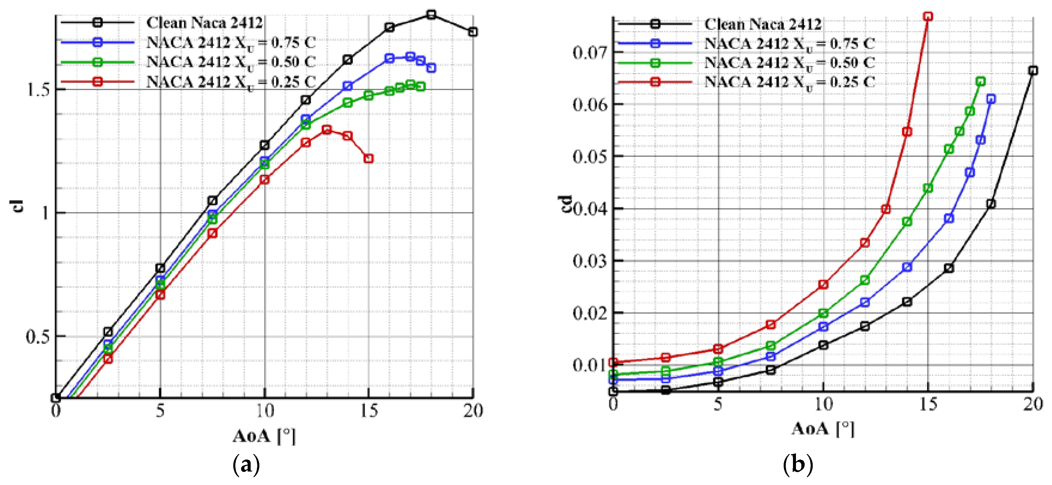
This subsection will test the relation between the step location and the critical angle of attack ${\alpha }_{cr}$, and whether the step has an effect on the onset of stall at a high Reynolds number.

Four different configurations of the NACA 2412 were tested. The first configuration is the clean NACA 2412, without any steps. The second, third and fourth cases incorporated a backward-facing step on the upper surface of the airfoil at $X_U/C=0.25, 0.5$ and 0.75, respectively. A wide range of angle of attacks $\alpha$ was tested on each of the four configurations to find the critical angle of attack ${\alpha }_{cr}$ at which the separated flow on the airfoil hinders the airfoil’s ability to create lift.

Figure 15a,b show the values of the lift coefficient $c_l$ and drag coefficient $c_d$ at different angles of attack $\alpha$. The curves in Figure 15a start with the linear relationship that extends up to an angle of attack of 10°. As the separated flow starts to become dominant around the airfoils, the relation between the lift coefficient and angle of attack becomes non-linear and quickly reaches the critical angle of attack ${\alpha }_{cr}$. It is shown in Figure 15a that the three cases of the stepped airfoil experienced an early onset of stall when compared to the case of the clean airfoil whose ${\alpha }_{cr}$ is approximately at 18°. While in cases of a backward-facing step at $X_U/C=0.25, 0.5$ and 0.75, the critical angle of attack was nearly at 13°, 17° and 17° respectively. Thus, the three cases of the installed step speeded up the onset of stall. The drag coefficient values shown in Figure 15b show that the stepped airfoils will experience higher dragging forces when compared to the clean airfoil. As the step location is shifted towards the leading edge of the airfoil, higher values of the drag coefficient are experienced, and they grow faster at lower angles of attack. These results show that installing a backward-facing step on the upper surface of the NACA 2412 degrades the overall stall behavior of the airfoil.

4. Conclusions

The study and analysis of the numerical results showed that a price has to be paid when using sliding morphing skin with a backward-facing step on the suction side of the airfoil. In comparison with the unchanged airfoil profile, employing a step on the suction side of the NACA 2412 airfoil had an adverse effect on the lift coefficient $c_l$, the drag coefficient $c_d$ and the critical angle of attack ${\alpha }_{cr}$. The location of the step $X_U/C$ prominently affected the aforementioned aerodynamic properties. The lift coefficient $c_l$ showed a direct relationship with the location of the step $X_U/C$, where the values of the lift coefficient continuously increased while shifting the step location from the leading edge to the trailing edge of the airfoil. On the other hand, the values of drag coefficient $c_d$ followed an inverse relationship with the step location $X_U/C$. Decomposition of the drag coefficient to its two main components showed a domination of the pressure drag coefficient over the viscous drag coefficient. This result shows that it is insufficient to use the skin friction coefficient as a sole tool of assessment, and only the pressure distribution curves will explain the relationship between the drag coefficient and the step location.

The four equations Transition-SST turbulence model was used to numerically model the transition of the viscous boundary layer from laminar to turbulent. The location of the step relative to the transition point affected the distribution of the pressure and the wall shear stresses, and consequently the variation of the lift and drag coefficients from one step location to the other.

By testing three configurations of the NACA 2412 with steps at different locations, and comparing the results to the unchanged airfoil, the backward-facing step speeded up the onset of stall and lowered the value of the critical angle of attack ${\alpha }_{cr}$. The case with a step at $X_U/C=0.25$ experienced an earlier stall condition when compared to cases with steps at $X_U/C=0.5$ and 0.75, which in turn have lower values of critical angle of attack ${\alpha }_{cr}$ compared to the clean airfoil.

As a conclusion, sliding skin with a backward-facing step on the suction side will degrade the aerodynamic performance of the airfoil, however, shifting the step from the leading edge towards the trailing edge relatively mitigate these adverse effects.