Review

Bio-Inspired Principles Applied to the Guidance, Navigation and Control of UAS

by
Reuben Strydom
1,2,*,
Aymeric Denuelle
1,3 and
Mandyam V. Srinivasan
1,2
1
The Queensland Brain Institute, The University of Queensland, Brisbane 4072, Australia
2
The School of Information Technology and Electrical Engineering, The University of Queensland, Brisbane 4072, Australia
3
Autonomous Systems Program, Commonwealth Scientific and Industrial Research Organisation (CSIRO), Pullenvale 4069, Australia
*
Author to whom correspondence should be addressed.
Aerospace 2016, 3(3), 21; https://doi.org/10.3390/aerospace3030021
Submission received: 28 April 2016 / Revised: 25 June 2016 / Accepted: 6 July 2016 / Published: 20 July 2016
(This article belongs to the Collection Unmanned Aerial Systems)

Abstract

:
This review describes a number of biologically inspired principles that have been applied to the visual guidance, navigation and control of Unmanned Aerial System (UAS). The current limitations of UAS systems are outlined, such as the over-reliance on GPS, the requirement for more self-reliant systems and the need for UAS to have a greater understanding of their environment. It is evident that insects, even with their small brains and limited intelligence, have overcome many of the shortcomings of the current state of the art in autonomous aerial guidance. This has motivated research into bio-inspired systems and algorithms, specifically vision-based navigation, situational awareness and guidance.

Graphical Abstract

1. Introduction

The past decade has seen an ever-increasing trend toward the use of autonomous robots for civil and defence applications. In particular, Unmanned Aerial System (UAS) have become a resourceful solution in many commercial flight operations. At present, there is a rich variety of UAS designs, ranging from medium to large fixed wing endurance aircraft (e.g., Global Hawk, Reaper, Scan Eagle) to smaller, more manoeuvrable, easily deployed multi-rotor platforms (e.g., Phantom Drone, Parrot AR Drone). Table 1 provides a brief overview of the main commercial and military UAS used nowadays, along with their specifications and intended applications.
The growing popularity of UAS can be largely explained by the increased capabilities they provide when compared to manned aerial navigation. Unmanned aircraft provide a safer and robust alternative for long-term flight operations, especially in performing monotonous tasks, and navigating in hazardous environments or cluttered scenes that would normally require a pilot’s full attention.
Current applications for UAS include monitoring and surveillance, search and rescue, disaster zone recovery, terrain mapping, structure inspection and agricultural crop inspection and spraying. These tasks often require flying at low altitudes and low speeds in urban or cluttered environments, thus encouraging the development of UAS that possess Vertical Take-off and Landing (VTOL) capabilities.

1.1. Current Limitations of Unmanned Aerial System (UAS)

Despite the existing diversity within unmanned aircraft, there are a number of limitations with the solutions that are currently available for UAS guidance. Examples of shortcomings include limited levels of autonomy (necessitating substantial human input), limited robustness to external disturbances, restricted endurance, and suboptimal human-machine interfaces [8]. In addition to the successful completion of specific missions, greater autonomy in aerial guidance requires navigation to be more self-reliant (with increased, independent onboard sensing), a deeper understanding of the surrounding scene (situational awareness), ultimately including an embedded ability to interact and respond appropriately to a dynamic environment that may change unpredictably.

1.1.1. Navigation

Currently, most manned and unmanned aircraft rely on satellite-based navigation systems (e.g., the Global Positioning System (GPS)). GPS is often used as the primary navigation sensor, and combined with an Inertial Measurement Unit (IMU) to fully determine the aircraft’s state (attitude, and 3D position and velocity). However, GPS-based navigation solutions remain limited by satellite signal coverage and also become unreliable, in terms of accuracy, in cluttered environments (e.g., dense forests, cities and locations surrounded by structures). Alternative solutions for navigation in GPS-denied environments include Simultaneous Localisation and Mapping (SLAM) and vision-based techniques, such as Vision-based SLAM (VSLAM) and optic flow.
SLAM is a popular technique that simultaneously constructs a map of an unknown environment and locates the robot within the completed map. The use of these map-based methods provides robots with the capacity to navigate in cluttered urban and indoor environments [8]. Traditionally, SLAM techniques used laser data to construct maps, however, VSLAM enables simultaneous localisation and mapping through the use of imaging sensors. Both SLAM and VSLAM provide accurate and robust GPS-free navigation through the use of natural landmarks. However, the selection and extraction of these landmarks in outdoor environments can be computationally expensive and is still a challenge for machine vision algorithms.
Another method to navigate in GPS-denied or challenging environments is to exploit radar [9]. Millimetre wave radar systems have been demonstrated to provide robust and accurate measurements, to be utilised as the primary sensor for SLAM [10,11]. The main drawback, at present, is that these radar systems have been confined to ground-based robots due to size, weight and power restrictions on UAS.
As alluded to above, in an effort to overcome the constraints of GPS, as well as reducing the computational burden of SLAM, vision sensors are increasingly being utilised in conjunction with biologically inspired algorithms (e.g., optic flow) for autonomous navigation in a variety of environments. Optic flow, which is the pattern of image motion experienced by a vision system as it moves through the environment, can be analysed to estimate the egomotion of an UAS. However, it is a challenge to obtain noise-free estimates of optic flow, and the resulting estimates of the position of the UAS will display errors that increase with time.

1.1.2. Situational Awareness

Safe navigation at low altitudes is only the first step to the future of UAS. Situational awareness is an important capability for enabling UAS to sense changes in dynamic environments and execute informed actions. Situational awareness is a requirement for applications such as collision avoidance, detection and tracking of objects, and pursuit and interception. The need for situational awareness in UAS becomes more apparent in the context of their integration into the civil airspace, where there is an increasing need for detecting and avoiding imminent collisions (e.g., Automatic Dependent Surveillance-Broadcast (ADS-B), FLARM (derived from “flight alarm”), Traffic Collision Avoidance System (TCAS), etc.). Although they have their place, sensors currently used for the detection of other aircraft (e.g., ground-based [12,13] or airborne [14,15] radar) can be bulky and expensive, and therefore, are often unsuitable for small-scale UAS.
Indeed, even with the present technology in early warning systems, during the period 1961–2003 there were 37 mid-air collisions in Australia, 19 of which resulted in fatalities [16]. It is interesting to note that out of the 65 aeroplanes involved, 60 were small single-engine aeroplanes, which are generally not equipped with the expensive early warning systems. Therefore, the development of more self-aware, vision-based, detection systems will also benefit light manned aircraft.
The goal for future autonomous aircraft may not be to simply avoid all surrounding objects. There is also a growing interest for robots to have an understanding of surrounding objects and the ability to detect, track and follow or even pursue them. For this, a UAS will need to be able to classify surrounding objects, which might include the object type or its dynamics. In essence, this will provide a UAS with the capability to determine whether an object is benign, a potential threat, or of interest for surveillance.

1.1.3. Intelligent Autonomous Guidance

Once UAS have the ability to acquire an understanding of their surroundings, for example an awareness of threats, the next step is to respond appropriately to the situation at hand. The control strategy for a potential collision will vary greatly depending upon whether the task involves flying safely close to a structure, or intercepting an object of interest. Future UAS will not only be required to assess and respond to emerging situations intelligently, but also abide by strict airspace regulations [17].
One way to better understand how these challenges could be addressed is to turn to nature. Flying animals, in particular insects, are not only incredible navigators (e.g., honeybees [18]), but also display impressive dexterity in avoiding collisions, flying safely through narrow passages and orchestrating smooth landings [19], as well as seeking out and capturing prey (e.g., dragonflies [20]). By investigating these animals through behavioural and neurophysiological studies, it is possible to develop simple and efficient algorithms for visual guidance in the context of a variety of tasks [18].

1.2. Vision-Based Techniques and Biological Inspiration

It is a marvel that flies instinctively evade swatters, birds navigate dense forests, honeybees perform flawless landings and dragonflies (such as the one seen in Figure 1) efficiently capture their prey. Nature has evolved to simplify complex tasks using vision as the key sense and utilising a suite of elegant and ingenious algorithms for processing visual information appropriately to drive behaviour. Animals such as insects display simple, yet effective, control strategies even with their miniature brains. These navigation (e.g., visual path integration, local and long-range homing, landing) and guidance (e.g., object detection and tracking, collision avoidance and interception) strategies are observable at various scales, and appear tailored specifically to each biological agent to suit its manoeuvrability, sensing ability, sensorimotor delay and particular task (e.g., predation, foraging, etc.).
Nature has demonstrated that vision is a multivalent sense for insects and mammals alike, with the capacity to enable complex tasks such as attitude stabilisation, navigation, obstacle avoidance, and the detection, recognition, tracking, and pursuit of prey or avoidance of predators. Thus, vision is likely the key to the development of intelligent autonomous robotics, as it provides the abundance of information required for these challenging tasks. This shared perception has led to a dramatic shift toward vision-based robotics.
One of the many benefits of vision is that it provides a passive sense for UAS guidance that (a) does not emit tell-tale radiation and (b) does not rely on external inputs such as GPS. Vision sensors are also compact, lightweight and inexpensive, thus enabling use in smaller-scale UAS. They also provide the capability for increased autonomy, because they can also be used for additional tasks such as object identification.
Following the pioneering work of Nicolas Franceschini, who was one of the first to translate the principles of insect vision to the development of ground-based robots that would navigate autonomously and avoid collisions with obstacles [21], a number of laboratories have progressed research in this area (e.g., [22,23,24,25]). These principles have been used to design and implement numerous bio-inspired algorithms for terrestrial and aerial vehicles, including safely navigating through narrow corridors (e.g., [26,27,28,29,30]), avoiding obstacles (e.g., [31]), maintaining a prescribed flight altitude (e.g., [23,32,33]), monitoring and stabilizing flight attitude (e.g., [34,35,36,37]), and docking (e.g., [38,39,40,41,42]) or executing smooth landings (e.g., [43,44,45,46]).
This paper will focus primarily on a summary of recent research in our own laboratory, with brief references to directly related work. It is not intended to be an exhaustive survey of the literature in the field. Other reviews pertaining to the field of UAS development, and biologically inspired robotics include Chahl [47], Duan and Li [48] and Zufferey et al. [24].

1.3. Objective and Paper Overview

In this paper, we will provide insights into some of the biologically inspired principles for guidance, navigation and control, which feature the use of unique vision systems and software algorithms to overcome some of the aforementioned limitations of conventional unmanned aerial systems. As the field of UAS research covers a large area, the work presented here will focus primarily on visually guided navigation of a rotorcraft UAS, on distinguishing between stationary and moving objects, and on pursuit control strategies (Guidance, navigation and control (GNC)). Novel GNC techniques are tested on a rotorcraft platform in outdoor environments, to demonstrate the robustness of vision-based strategies for UAS.
Section 2 provides an overview of the experimental platform with a description of the rotorcraft UAS, the vision system and the control architecture. Optic flow and view-based navigation techniques are discussed in Section 3; an example of situational awareness, by determining whether an object in the environment is moving or stationary, is covered in Section 4; and interception guidance strategies are explained in Section 5. Finally, Section 6 presents concluding remarks and future work. Each section will begin with the description of a biological principle, followed by a description of how the principle is applied to rotorcraft guidance.

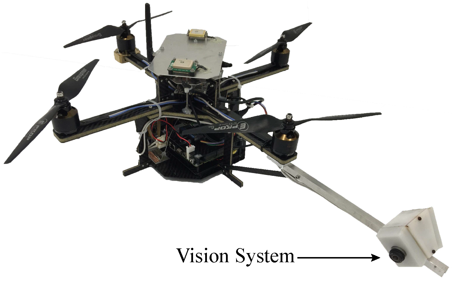
2. Experimental Platform

With a growing interest in the vast military and civilian applications, UAS have been deployed in applications ranging from environmental structure inspection to search and rescue operations. Many UAS applications now require the ability of flight at low altitudes, near structures and more generally in cluttered environments. For these reasons, rotorcraft have gained popularity as they can perform a large variety of manoeuvres, most notably vertical take-off, landing and hover.

2.1. Overview of Platform

Our experimental platform is a custom built quadrotor in the QUAD+ configuration, as shown in Figure 2. The control system incorporates a MikroKopter flight controller and speed controllers for low-level stabilisation and an embedded computer (Intel NUC i5 2.6 GHz dual-core processor, 8 GB of RAM and a 120 GB SSD) for the onboard image processing, enabling real-time, high-level guidance and control (roll, pitch, throttle) of the UAS. The platform additionally has a suite of sensors including a MicroStrain 3DM-GX3-25 Attitude and Heading Reference System (AHRS) for attitude estimation, a Ublox 3DR GPS and Swift Navigation Piksi Differential GPS (DGPS) for accurate ground truth results, and a novel bio-inspired vision system.

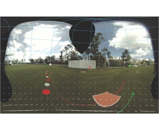
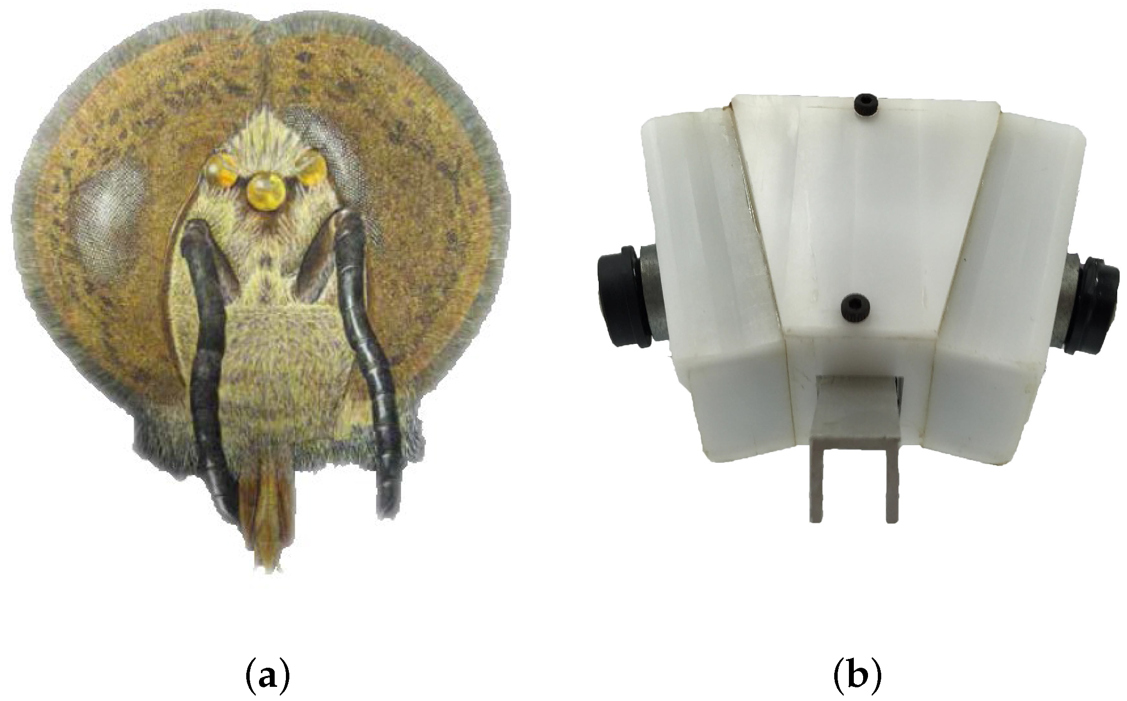
2.2. Biologically Inspired Vision System

The biologically inspired vision system on our flight platform is a design inspired by the insect eye. The left and right compound eyes of a honeybee (Figure 3a) each cover an approximately hemispherical field of view, thus providing near-panoramic vision, which is useful for accurate and robust estimation of egomotion, as well as for detecting objects of interest in various directions. The compound eyes also feature a 15 overlap in the front, which could provide stereo vision at close ranges—although this is yet to be confirmed [18,49].
The vision system used in our flight platform, as demonstrated by Figure 3b, embodies the functionality of the insect compound eye by using two Point Grey Firefly MV cameras with Sunex DSL216 fisheye lenses. Each camera has a Field of View (FOV) of 190 . They are oriented back-to-back with their nodal points 10 cm apart, and are tilted inward by 10 to provide stereo vision in the fronto-ventral field of view. The cameras are calibrated using a similar method to Kannala and Brandt [50], and the images from the two cameras are software synchronised and stitched together to obtain a near-panoramic image with a resolution of 360 by 220 pixels. This image is then converted to grey scale and resized to 360 by 180 pixels to compute panoramic optic flow, and from it the egomotion of the aircraft. In addition, stereo information is used to estimate the height of the aircraft (HOG) above the ground. Due to the relatively small baseline between the cameras (10 cm), the operating range is within 0.2–15 m.

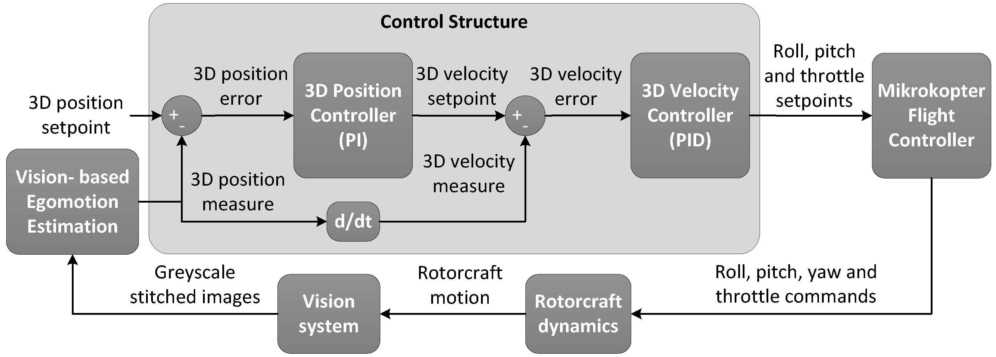
2.3. Control Architecture

The high level to low level control architecture of the quadrotor utilises two cascaded Proportional-Integral-Derivative (PID) controllers for position and velocity control. The objective is for the quadrotor to minimise the error between the 3D position set point and the currently estimated position.
As illustrated in Figure 4, the position error is fed into a PID controller that generates a velocity command. This velocity command is compared with the aircraft’s measured velocity to generate a velocity error signal, which is cascaded into another PID controller that generates appropriate changes to the roll, pitch and throttle setpoints. These setpoints are the inputs for the Mikrokopter flight controller. Finally, the output of the flight controller, together with the dynamics of the aircraft, determine the quadrotor’s motion.

3. Navigation

Navigation is an essential first step for increased autonomy in UAS. As stated previously, this requires knowledge of an accurate state of the aircraft (e.g., attitude, and 3D position and velocity) not only for navigation but also for more complex guidance tasks. Increasingly, however, applications require UAS to navigate at low altitudes and in cluttered environments, which can cause sensors, such as GPS, to become unreliable. This current overreliance on GPS limits the autonomy of UAS in GPS-denied locations.
Vision-based navigation approaches have demonstrated their practicality for overcoming some of the limitations of traditional GPS sensors. In Section 3.1, we will discuss how insects use optic flow for their navigation and bio-inspired implementations for UAS GNC. Section 3.2.1 will cover holistic (view-based) techniques that significantly reduce the complexity for local homing. Finally, Section 3.3 introduces works toward vision-only navigation.

3.1. Optic Flow-Based Navigation

Optic flow is the pattern of image motion that a vision system experiences when its owner moves through the environment [17]. It can be described quantitatively as a set of vectors, commonly termed the “optic flow field”, that characterise the direction and extent of motion of each part of the image [52]. The optic flow field that an animal experiences is rich in information about the animal’s motion in the environment [53,54]. Clockwise image motion of the entire panoramic image, for example, indicates a counter-clockwise rotation (yaw) of the animal; downward image motion in the left visual field and upward image motion in the right visual field indicates a clockwise roll; forward image motion in the upper visual field and backward image motion in the lower visual field indicates an upward pitch; and expansion of the image in any part of the the visual field indicates a translatory motion of the animal in that direction [53,54]. Furthermore, during translatory egomotion, the magnitude of the optic flow vector in each region of the image provides information on the distance to the nearest object in that direction [19]. Flying insects have evolved to exploit optic-flow information to stabilise and control flight attitude, control flight speed, avoid obstacles, fly safely through narrow passages, measure distance flown, and execute smooth landings [18,19].
Although we do not yet fully understand the neural processing mechanisms by which bees and other flying insects compute optic flow and analyse it to estimate their motion through the environment, there are bio-inspired engineering solutions that have successfully adopted the underlying principles for aircraft guidance.
In the engineering literature, several key algorithms have been devised for the computation of optic flow, of which the most famous algorithms include Lucas and Kanade [55] as well as Horn and Schunck [56]. These methods represent useful techniques for computing the optic flow field, which can subsequently be analysed to estimate the egomotion of the UAS [19]. Applications for optic flow are numerous, for example it has been utilised for speed regulation [29], terrain following [32,57], monitoring wheel slip on the Mars Rovers [58], collision avoidance [31] and localisation for many Simultaneous Localisation and Mapping (SLAM) systems [45].
Our optic flow algorithm, an engineering-based approach described in [46,59], utilises an intensity-based pyramidal (similar in principle to that described by Lucas and Kanade [55]) block-matching algorithm. The panoramic images provided by our vision system, as discussed in Section 2.2, are segmented into a grid of 25 × 15 regions in which 7 × 7 pixel image patches are randomly chosen within each grid square. A 7 × 7 pixel search region is then used to find matches between frames, to obtain the optic flow field. To estimate the egomotion from this optic flow field, an iterative search algorithm is used to obtain the combination of 3D translation and 3D rotation that best explains the measured flow field [46,59]. To reduce the complexity of the egomotion computation, the ground is assumed to be a plane; however, the performance of the egomotion estimation could be compromised if used over significantly uneven terrain [46,59]. Our algorithm characterises the aircraft’s egomotion by delivering two vectors: (1) a 3D rotational vector, which specifies the direction of the axis of rotation and the magnitude of this rotation, and (2) a 3D translational vector which specifies the direction of the translation, where the magnitude of this vector is scaled to the aircraft’s height above the ground (HOG). The HOG is measured by the on-board vision system, using stereo information, as described in Section 2.2. This scale factor is then used to compute the translation in absolute distance units.
The stereo computation of the HOG is performed in a way analogous to the optic flow computation. It also incorporates a pyramidal block-matching algorithm through the use of 7 × 7 texture patches and sub-pixel refinement; however, the stereo algorithm applies a 7 × 3 pixel search region (instead of 7 × 7 pixels). This reduced search window biases toward horizontal motion between the two patches, reflecting the half-pixel tolerance for the epipolar matching. The vector pertaining to a valid match is then triangulated to estimate the range to the ground plane and trigonometrically converted to a height over ground. The conversion of the range vector to a height over ground, however, requires knowledge of the roll and pitch of the aircraft, which in most cases is specified by the Attitude and Heading Reference System (AHRS). Once all the valid matches have been triangulated to compute range, the range values are accumulated into a histogram, which is used to apply outlier rejection. Finally, after the removal of outliers, the median value of the histogram, encompassing 68% of the values, provides the true stereo height estimate.
The optic flow and stereo algorithms have been tested onboard a rotorcraft UAS in a number of applications, such as visual odometry, drift-free snapshot-matching-based navigation and autonomous landing, which are discussed in greater detail in the following sections. Our stereo vision system is also used for the pursuit of a ground target, as explained in Section 5. In principle, optic flow can be computed between two successive image frames, referred in this paper as frame-to-frame optic flow (OF-FTF), or computed between the current image and a reference image, which will be termed optic flow-based snapshot matching (OF-SM).

3.1.1. Visual Odometry
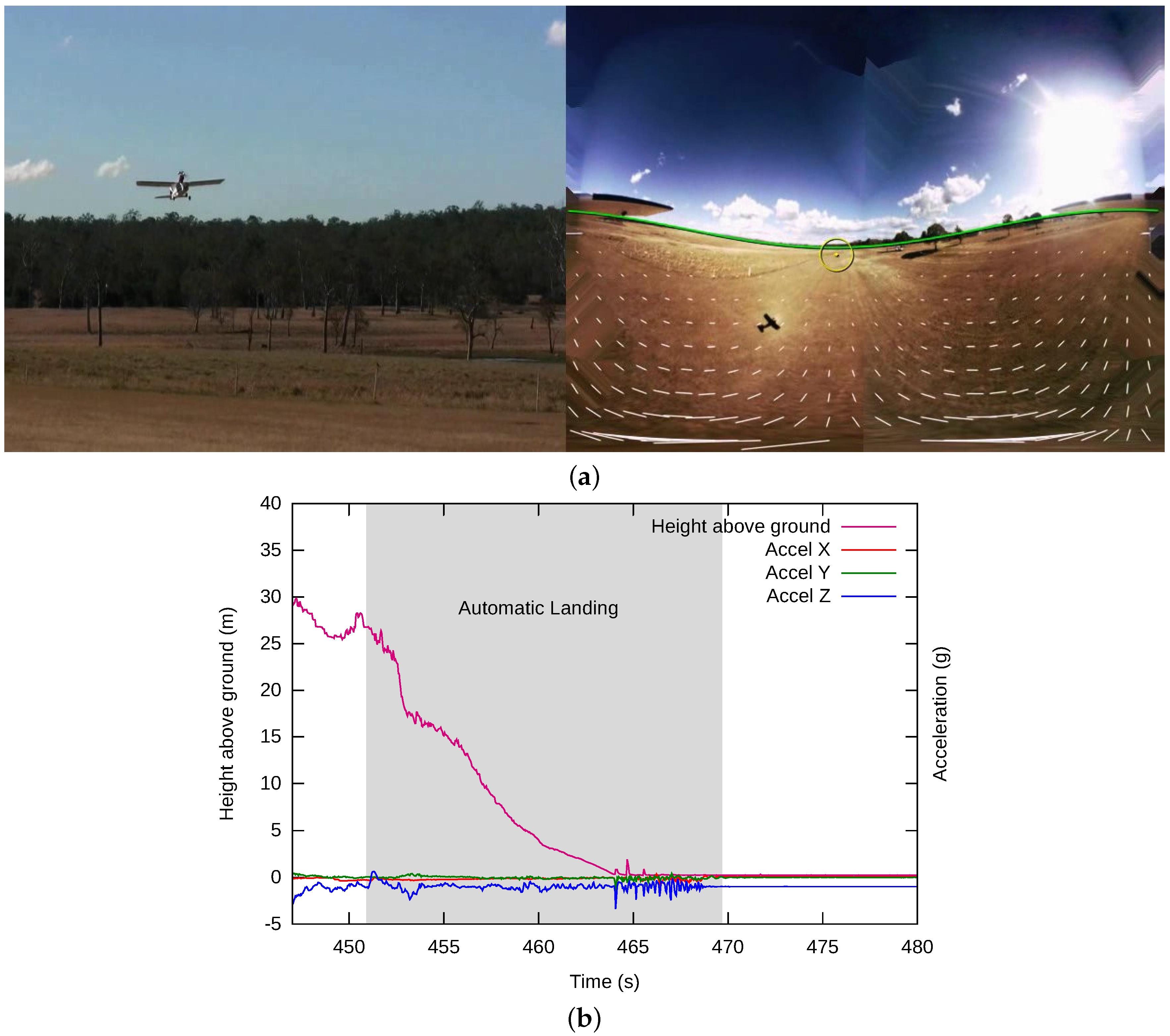
In the animal world, the ability to perform visual odometry has been demonstrated in honeybees. The demonstration was accomplished by observing and video-recording the dances that bees perform when they return to their hive after discovering a new food source. The bee oscillates its abdomen from side to side during a phase of the dance known as the "waggle phase", which conveys to its nest mates the direction of the food source, and the distance they must fly to reach it [60]. The duration of the waggle phase is proportional to the distance of the food source—the farther away the food source, the longer the waggle duration. The bee’s nest mates use the information from this waggle duration to navigate to the new food source. Evidently, honeybees possess an ‘odometer’ that informs them about how far they have flown.
To investigate the nature of the honeybee’s odometer, [61,62] trained bees to fly directly from their hive into a short, narrow tunnel that was placed very close to the hive entrance (Figure 5). The tunnel was 6 m long and 11 cm wide. A sugar water feeder was placed at the far end of the tunnel. The walls and floor of the tunnel were lined with vertical stripes. The dances of bees returning from this feeder were video-filmed. Incredibly, these bees signalled in their waggles a flight distance of approximately 200 m, despite the fact that they had flown only 6 m (Figure 5a). One explanation for this exaggerated distance estimate would be that the bees were gauging the distance they had flown by measuring the total extent of image motion that they had experienced during the flight from the hive to the feeder, i.e., by integrating, over time, the optic flow that they had experienced en route. The proximity of the walls and floor of the tunnel would greatly magnify the optic flow that they experienced, in comparison with what would normally occur when foraging outdoors. To test this hypothesis, the bees were flown in a tunnel of the same dimensions, but lined with axial stripes, which induce no optic flow because the flight is in a direction parallel to the stripes. The bees then produced no waggles in their dances (Figure 5), signalling the experience of a very short journey. Evidently, in this case, the absence of optic flow caused the odometer to barely tick over [61]. These studies, taken together with evidence from other kinds of experiments [18] provide strong evidence that the bee’s odometer is visually driven, and delivers a measure of distance flown by integrating, over time, the optic flow that is experienced during the journey.
Visual odometry, as performed by the honeybee, is a useful tool for UAS navigation and has the potential to reduce the number of sensors currently used on autonomous vehicles. Visual odometry has been a popular method to compute the motion of ground and aerial vehicles through stereo-based (e.g., [63,64,65,66,67,68]), homography-based (e.g., [69,70]) and optic-flow-based methods (e.g., [45,59,71,72,73]). Currently, the majority of methods are tested on gound-based vehicles, however, studies that demonstrate visual odometry on UAS include [59,68,69,71]. The vision-based navigation technique investigated by Strydom, et al. [59], demonstrates that the information from OF-FTF and stereo can be used to estimate the egomotion of a UAS from one image frame to another. To perform visual odometry, the frame-to-frame egomotion vectors are summed sequentially to obtain the current pose (3D position and 3D orientation) of the aircraft. This process is known as “path integration” [18,74].
The outdoor field tests presented in [59] demonstrate that this approach can be used successfully for robust navigation of a UAS along a pre-defined trajectory (UAS visual odometry flight video available at: https://youtu.be/I1QDAHEzlj8). In these tests, the rotorcraft UAS took-off autonomously, navigated a square trajectory and landed without any human intervention. These experiments demonstrate that this vision-based odometry technique is capable of returning the aircraft to its take-off point with a mean error of 0.8 m after navigating a 10 × 10 m square trajectory, at a height of 3 or 5 m, representing a total travel distance of 46–50 m, as shown in Figure 6a,b. This represents an average error of approximately 1.7% of the total path length over all of the tests that were conducted. Table 2 provides a comparison of various visual odometry solutions. Note, that this is only a guide as each method is tested under varying conditions and hardware configurations.
This visual odometry algorithm offers many benefits for visual navigation and could, in principle, be used on a variety of autonomous platforms (e.g., multi-rotor crafts, fixed-wing aircraft and ground robots), without requiring GPS or computationally expensive feature extraction. As with any integrated signal, the main limitation of the OF-FTF technique is that the error in the positional increases with distance travelled due to the noise that is inherent to the motion estimate at each step.

3.1.2. Landing

Flying insects appear to have evolved simple and elegant strategies for orchestrating smooth landings. Honeybees were video-filmed as they approached and landed on a horizontal surface, and their trajectories were reconstructed in 3D [61]. Analysis of the trajectories revealed that, during the landing process, the bees adjust their flight speed in such a way as to keep the velocity of the image of the ground constant as they approach it (Figure 7). Keeping the image velocity of the ground constant automatically ensures that the flight speed is progressively reduced as the ground is approached, and that it is close to zero at touchdown. The attractive feature of this landing strategy is that it does not require information about the distance to the ground, or the speed of the insect, at any instant of time. All that is required is a vision system that is capable of measuring the optic flow that is generated by the ground. A subsequent study has shown that a generalised version of this strategy of holding the optic flow constant can be adopted for landing on a surface of any orientation, be it horizontal, vertical or oblique [18].
This simple strategy can be implemented into UAS for achieving robust landing without the need for additional sensors to measure the height above ground or the velocity (e.g., by using GPS). We note, however, that this strategy requires that the speed of the aircraft approach a value of zero close to touchdown. Therefore, it is ideally applicable to an aircraft that is capable of hover, such as a rotorcraft (e.g., [23,44,45]), but not to a fixed-wing aircraft that would stall at low speeds. One approach to circumvent this problem is to use a small, lightweight aircraft that implements the bee landing principle and stalls at the end of the landing approach, but at a height very close to ground, thus avoiding damage [43]. This approach can be risky in a heavier aircraft that carries a valuable payload.
A modified version of the honeybee’s landing strategy has been successfully applied to guide the landing of a larger fixed-wing model aircraft (Autonomous landing of a fixed-wing aircraft video available at: https://youtu.be/U9iy1B5QG-0) [46]. There the flight speed is held constant (rather than reducing the velocity, as in the case of the honeybee), and the descent rate (rate of change of height) is controlled by measuring and regulating the rate of increase of optic flow, which can be set to achieve a fixed descent time, if desired. This mode of descent control is applied to reduce the HOG from 15 to 4 m. Below 4 m, stereo-based height information is used to control the descent to the point of touchdown. Stereo information provides accurate height readings below 4 m because this height range is compatible with the stereo baseline and the resolution of the cameras. In this height range it is difficult to derive reliable information from optic flow, because the magnitude of the optic flow is too large to permit accurate measurement—recall that the fixed-wing aircraft approaches the ground at a constant speed, which means that the magnitude of the optic flow increases as the ground is approached.
Figure 8a shows an example of an automatic landing. The left-hand panel shows an external view of the landing aircraft and the right-hand panel shows the panoramic image captured by the vision system, with the superimposed optic flow vectors. Figure 8b shows the height profile during the landing. The initial descent from 40 to 15 m is open loop, and is achieved by setting the throttle to a minimum and the pitch to −25 . After the HOG has dropped to 15 m (as indicated by stereo), the rate of descent is controlled through closed-loop regulation of the optic flow, and below 4 m the descent rate is controlled by using stereo to monitor the height, as described above. Further details are available in [46].

3.2. Drift-Free Hover Stabilisation and Navigation via Bio-Inspired Snapshot Matching

Hoverflies and dragonflies are living proof of the ability of insects to achieve stable hover at any desired location, with minimal drift. It is thought that this form of station-keeping is achieved by acquiring a panoramic snapshot of the visual environment at the desired hover location, and using this memorised snapshot to detect and correct any drift from the hover location by detecting and analysing the difference between the current image and the memorised snapshot. Furthermore, drift-free navigation can be achieved by first memorising a visual route, defined by a sequence of snapshots, and then following this learned route back to the initial location.

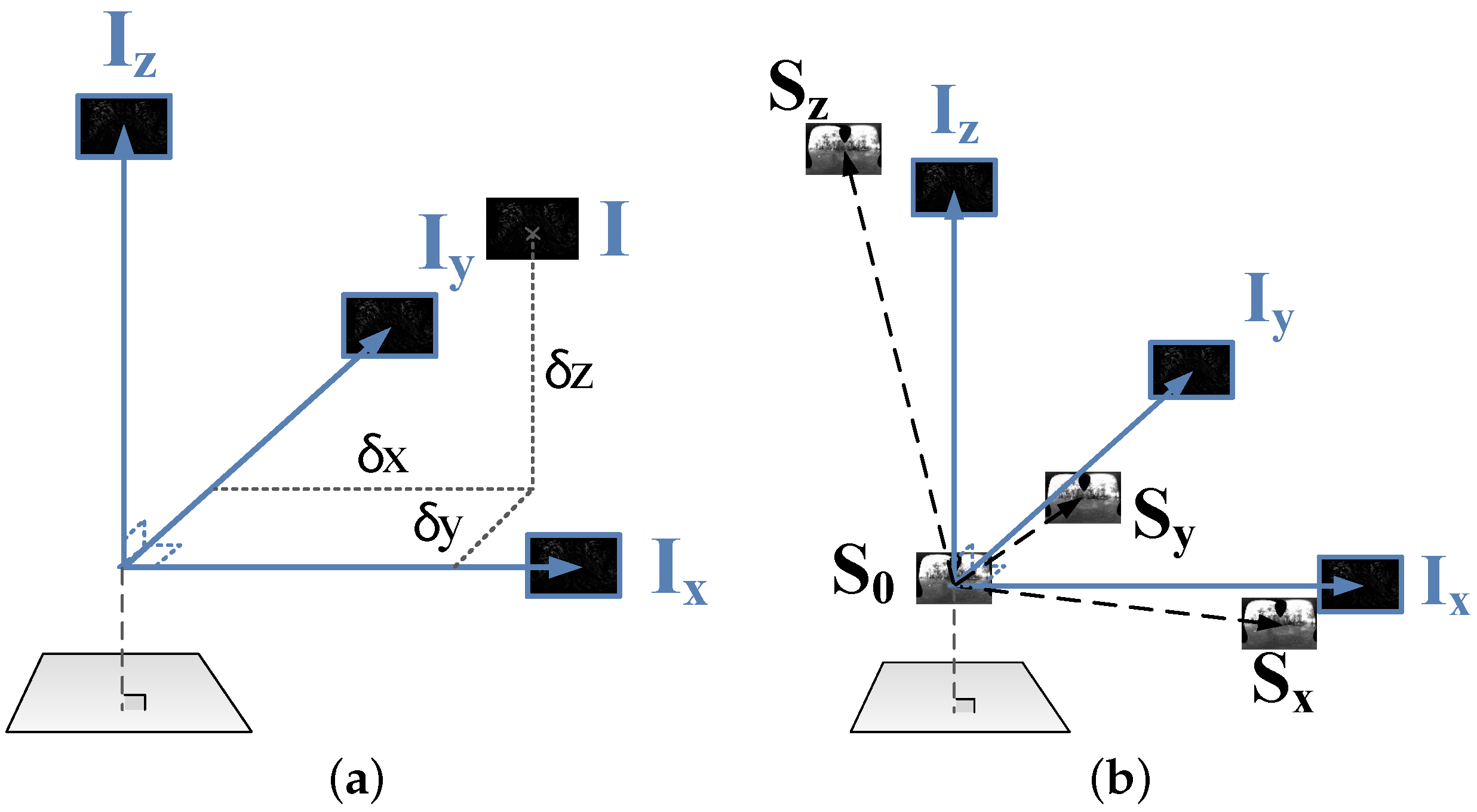
3.2.1. Control of UAS Hover through Image Coordinates Extrapolation (ICE)

Autonomous hover has been successfully demonstrated in indoor environments through the use of lightweight devices (such as infrared [80] and ultrasonic sensors [81]) but also through techniques based on image servoing [82,83,84,85,86]. However, vision-based methods typically require the use of artificial setups that constrain their applicability in outdoor environments [87]. Although outdoor hover has been demonstrated with a good accuracy level in [88,89], VSLAM techniques require a sufficient processing capability to extract and track hundreds of features.
Less computationally intense vision-based methods for stabilising hover rely on the image difference function (pixel-wise difference between a reference snapshot and the currently experienced view) [18]. For small displacements around a reference location (home), image differences increase smoothly and monotonically in natural environments [90]. Gradient-based guidance techniques [60] can be derived from the image difference function (IDF) to maintain the hover location by following the direction along which the image differences decrease. However, such schemes require complex, and therefore undesirable exploratory movements at each time step to sense the environment and its image gradient. In addition to being sensitive to odometric errors, techniques that use gradient descent in image differences do not provide a direct estimate of the distance to home.
Denuelle et al. [91] introduces a novel view-based method, based on the IDF, that does not require any exploratory movements or the use of an odometer, once the process is initialised. This approach, the Image Coordinates Extrapolation (ICE) algorithm, assumes that any location around the reference position can be described by a difference image (pixelwise difference between the reference snapshot and the current view), and that this difference image is a linear combination of three reference difference images taken around the reference location (for navigation in 3D environments). The current difference image is projected onto the reference difference image frame (built from snapshots taken at the reference location), which provides relative coordinates to the home position, as shown in Figure 9. This approach was applied to the stabilisation of hover of a small-size rotorcraft UAS in natural environments (External ICE-based closed-loop hover video available at: https://youtu.be/ZDPiF5Bfyj4, Onboard ICE-based closed-loop hover video available at: https://youtu.be/X_tp4F9v8_I) in [92]. The ICE algorithm provides a computationally efficient and a drift-free method to fully estimate the rotorcraft’s state (3D position and velocity) and maintain accurate hover in unknown environments.

3.2.2. Control of UAS Hover Through Snapshot Matching

Denuelle, et al. [93] uses the snapshot concept in the computation of optic flow to stabilise the control of hover of a rotorcraft UAS. Optic flow is a popular technique for the real-time stabilisation and control of small-size rotorcraft [23,31,45,94,95,96,97].
In the approach proposed in [93], the optic flow is estimated between a reference snapshot (panoramic image) and the current camera frame. The use of a reference snapshot eliminates cumulative odometric errors and prevents long-term drift in the visual estimates [93], thus providing drift-free control of hover, as shown by the blue line and shading in Figure 10. Although the snapshot-based method remains limited by the size of the catchment area (the 3D region within which position estimates can be accurately determined and lead to successful hover maintenance), results from closed-loop flight experiments (OF-SM based closed-loop hover flight (external view) video available at: https://youtu.be/5jACjzUcA7Y) demonstrate better hover performance than approaches that are based on traditional frame-to-frame measurements of optic flow, such as the technique described in Section 3.1, which is depicted by the green line and shading in Figure 10. Compared to [98], the full rotorcraft’s state (both 3D position and velocity) is estimated by using the optic flow computed with reference to the initial snapshot only.

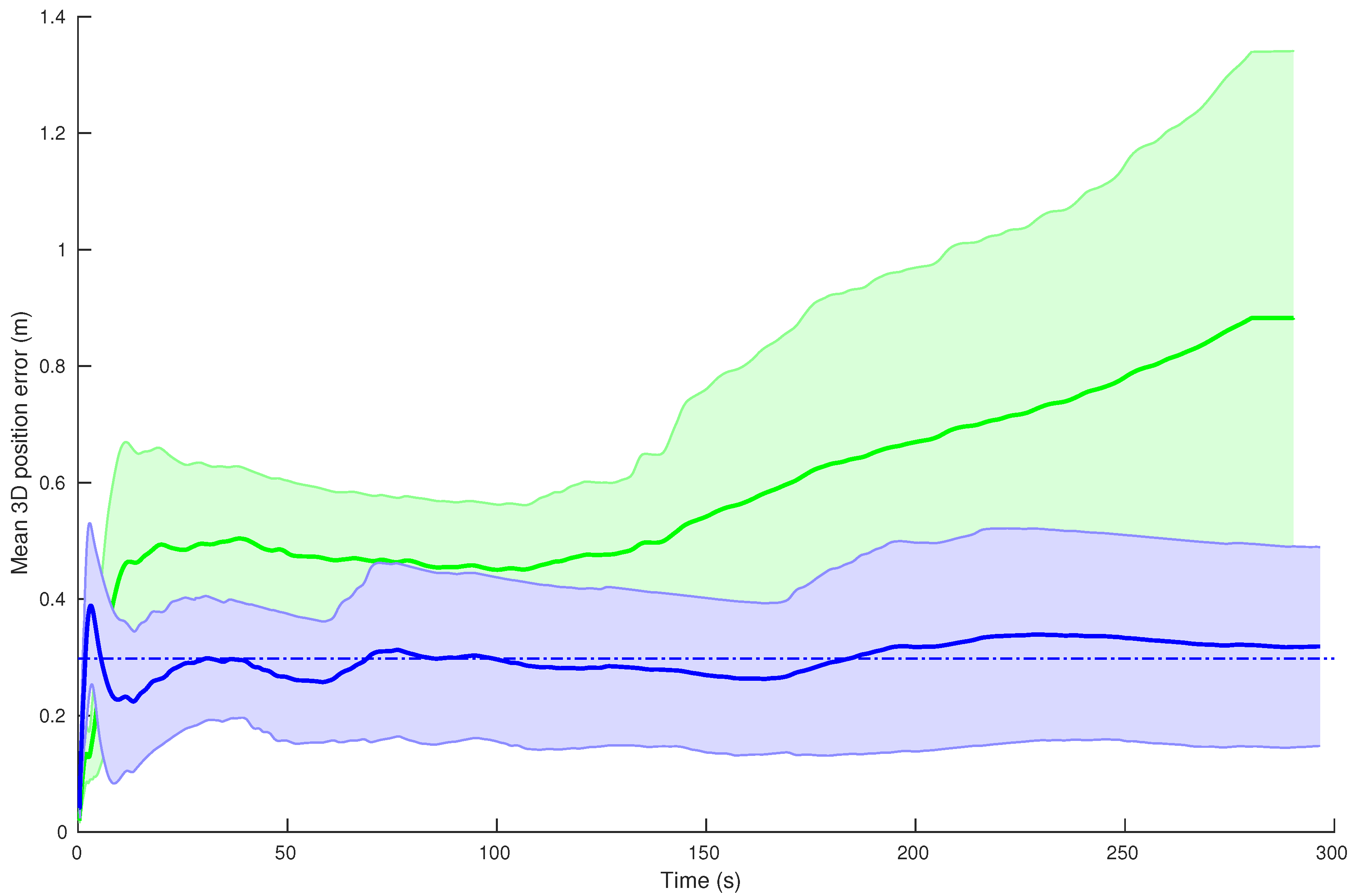
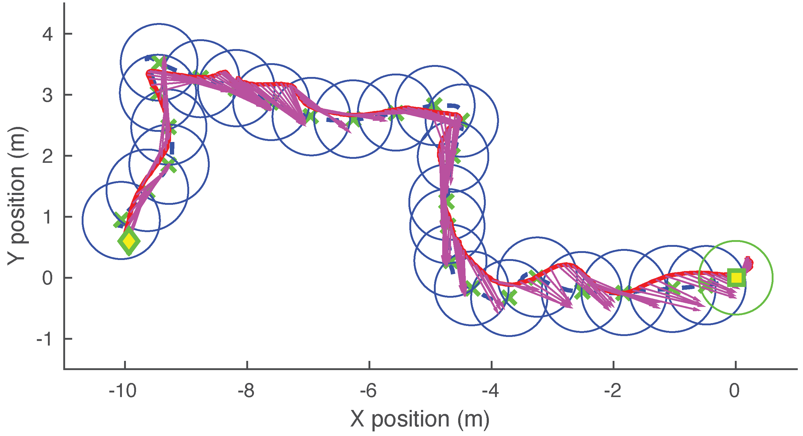
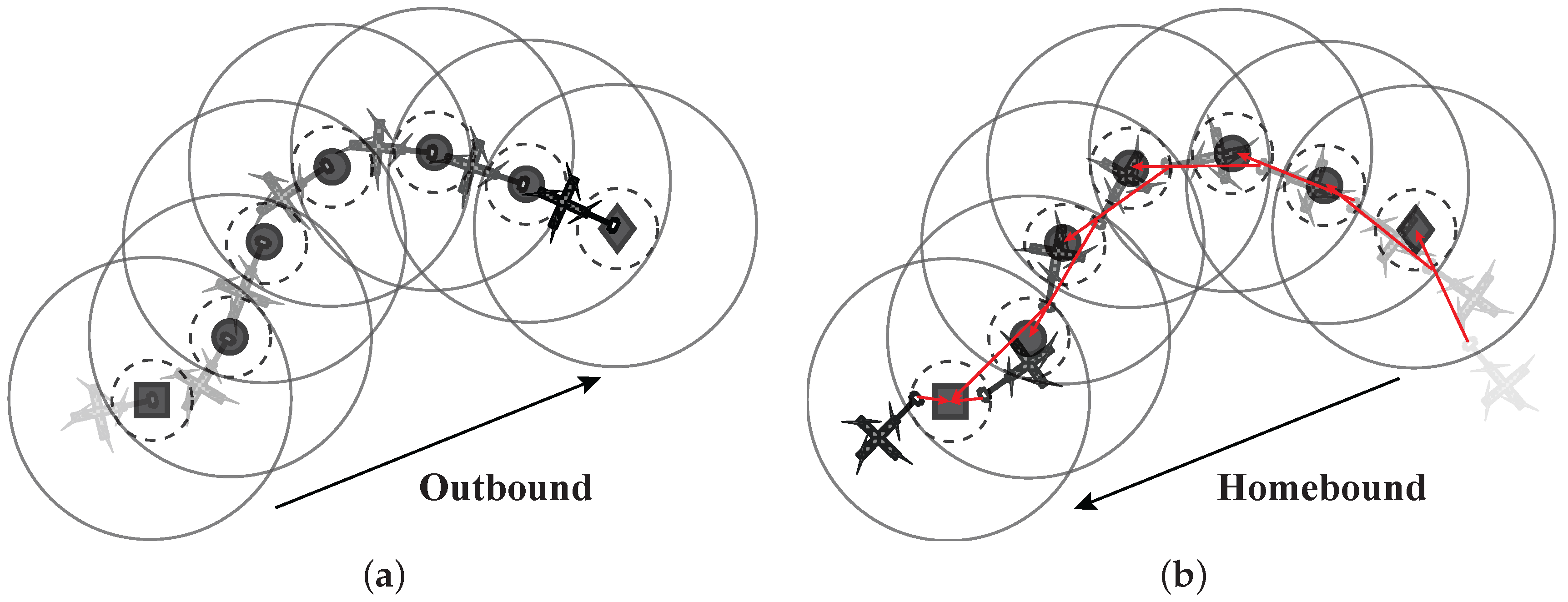
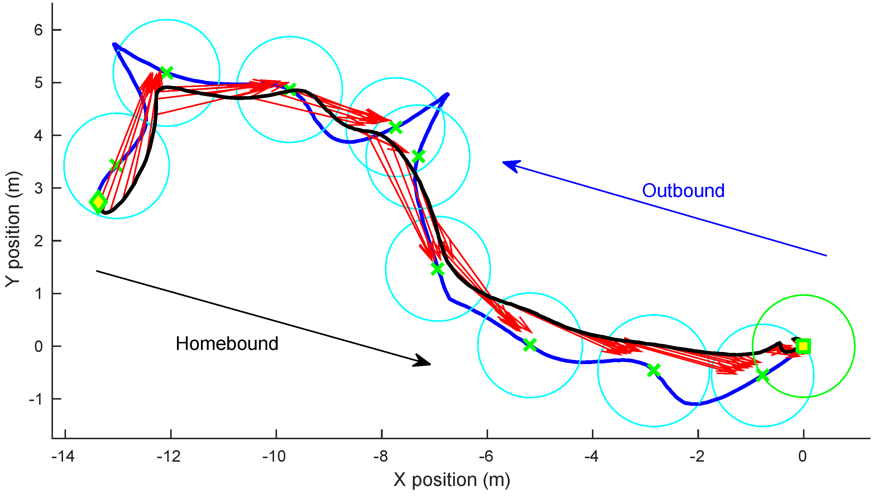
3.2.3. Control of UAS Navigation Through Snapshot Matching

The snapshot-based approach can also be applied to autonomous navigation. Instead of relying purely on dead reckoning [31,45,59], navigation from a location A to another location B can be performed by acquiring panoramic snapshots at a series of waypoints along the route from A to B in a “learning” phase. If each waypoint is considered to be a hover location and if the waypoints are sufficiently closely spaced that their catchment areas overlap, then the route can be followed by moving from one catchment area to the next.
Traditionally, a visual route is composed of a sequence of discrete waypoints, representing visual locales and defined by either global (whole image, image histogram) [99,100,101,102,103,104] or local descriptors extracted from input images (geometric features, SIFT points, average landmark vectors, etc.) [105,106,107,108,109,110,111].
Denuelle and Srinivasan [112] proposes a lightweight navigation framework where the UAS learns a visual route to a goal by memorising a sequence of snapshots at selected waypoints along the route, and returning home by retrieving, in reverse order, the snapshots corresponding to the sequence of waypoints. This minimalistic technique for route learning and navigation is demonstrated in Figure 11a,b. Both the route learning and navigation modules make use of the snapshot-based method (see Section 3.2.2) to estimate the rotorcraft’s egomotion relative to a memorised panoramic snapshot. The egomotion information is used to either select whether the current camera frame should be memorised as a new snapshot waypoint (route learning), or to estimate the 3D state (position and velocity) of the UAS relative to the position corresponding to a snapshot acquired previously along the navigated route. In the proposed scheme, successive snapshots are selected so that their catchment areas (CAs) overlap by a large amount (at least 50%), which enables a simple navigation strategy. Indeed, as soon as the UAS reaches the center (or its vicinity) of the current CA, it is also located within the next snapshot’s CA, thus enabling the UAS to update its next intermediary goal location. An example of the homing journey conducted in a field test is presented in Figure 12. Despite the simplicity of the route description, drift-free navigation is achieved. The technique also leads to route optimisation and the subsequent reduction of the number of memorised snapshots required to describe a route between two locations.
Another snapshot-based navigation strategy, presented in [113], makes use of a visual route composed of a series of snapshot-vector duples (each memorised snapshot is associated with a vector pointing toward the previous CA, as illustrated in Figure 13a). This approach progressively builds a minimal route description that enables efficient snapshot-based navigation between two given locations, without requiring path integration. As in [112], navigation back home is achieved by retrieving each memorised snapshot’s location in reverse order, but a faster path optimisation is achieved (see Figure 14 for an example), with significant route reduction when travelling repeatedly between two familiar locations. When the final route description has been achieved, the number of learnt snapshots is reduced because the route is more direct.

3.3. Vision-Only Navigation

One limitation of the methods presented here, as is common to most vision-based navigation algorithms, is the need for an Inertial Measurement Unit (IMU) to estimate the orientation of the aircraft. This information was used to set the direction of the normal to the ground for the optic flow and stereo measurements. IMUs, however, are prone to noise induced drift, which compromises performance [114]. Indeed, the long-term drift in the OF-FTF estimates would diverge even faster if the IMU provides an incorrect attitude estimate.
Future work in autonomous vision-based navigation could see the use of a pure vision system that uses optic flow information, the horizon profile or the use of an image difference function to determine the orientation of the UAS. The horizon-sensing algorithms developed in [36,115], designed for a fixed wing aircraft travelling at a higher altitude than a quadrotor, could potentially be adapted to suit low altitude flight. More recently, as shown in [37], a 3D sky compass can be used to achieve robust estimation of the UAS attitude in low altitude scenarios. It could form part of a purely vision based navigation technique, if used in conjunction with our egomotion algorithms.

4. Situational Awareness

Situational awareness in a dynamic environment is key for various UAS applications, for example to avoid potential accidents. Since safety is a growing concern for small but powerful autonomous vehicles as they increase in numbers, awareness of the UAS surroundings is paramount. One such requirement is to evaluate the risks posed by surrounding objects, either for the purpose of ignoring, pursuing or for avoiding collisions with them [116,117]. One way to assess whether an object might pose a threat would be to determine if the object is moving or stationary.

4.1. Object Detection and Tracking

Before determining whether an object is a threat or not, it must first be detected. There are a multitude of techniques for object detection. Infrared (IR) sensors have been used to detect a static target in an indoor environment (e.g., [80,118]). Such systems are of restricted utility, as they are unsuitable for outdoor use. Motion contrast, typically measured through the use of dense optic flow, is another method utilised in [119] to detect a moving target. Dense optic flow has the benefit that the target does not have to be detected a priori, but this method is computationally expensive and cannot detect static objects. Colour-based segmentation has been shown to be useful for the detection of both static and moving targets without knowledge of the shape or size—although it does require the specification of a reference colour. As the detection of an object is only seen as an intermediate step, colour segmentation seems the most appropriate choice for the ability to test awareness algorithms. Colour-based detectors typically use a seeded region-growing algorithm to ensure that the entire object is detected, even in varying lighting conditions. This method also allows for slight colour gradients across the object in an outdoor environment. Once the object has been detected, the next steps are to determine if the object is a risk and then to pursue or avoid it.
Here we will focus on two principal challenges that need to be addressed after the target is detected from a moving vision system: first, determining whether the target is stationary or moving ("target classification"); and, second, as described in Section 5, adopting an appropriate control strategy for pursuing or following the target.

4.2. Target Motion Classification: Determining Whether an Object Is Moving or Stationary

Pinto, et al. [120] describes three main techniques for determining whether an object is moving: using background mosaics, identifying areas of motion contrast and the use of optic flow-based geometrical methods. Arguably, the most popular of these methods is the use of motion contrast, which deems the object to be moving if there is a difference between the motion of its image and that of its immediate background.
Detecting moving objects using motion contrast is fairly trivial when the vision system is static, whereby methods such as background subtraction [121] or frame differencing [122] can be employed. However, the problem becomes much more challenging when the vision system is also in motion. Motion contrast techniques that are used for the detection of moving objects onboard a moving platform include background subtraction [123,124,125] and optic flow based methods [119,126,127].
Motion contrast is a reliable method for detecting a moving object if the object is approximately at the same distance from the vision system as the background. However, when the object is at a different distance, such as an elevated ball, motion contrast will be present even when the object is stationary. This is a major limitation of many current techniques that rely solely on motion contrast to determine whether an object is moving. The following sections will demonstrate two techniques that overcome the limitations of motion contrast, one that uses an epipolar constraint and a second that additionally tracks the size of the object’s image.

4.2.1. Using the Epipolar Constraint to Classify Motion

This approach computes the egomotion of the moving platform from the global pattern of optic flow in the camera image, and looks for regions in the image where the local direction of optic flow is different from that expected from a stationary environment [128]. This can be thought of as an epipolar constraint. The epipolar constraint has also been utilised in [129] to detect independently moving objects in non-planar scenes. The study by Strydom, et al. [128], describes a vision-based technique for the detection of moving objects by a UAS in motion. The technique, which is based on measurement of optic flow vectors, incorporates the following steps to determine whether an object is moving or stationary:
  • Compute the egomotion of the aircraft based on the pattern of optic flow in a panoramic image.
  • Determine the component of this optic flow pattern that is generated by the aircraft’s translation.
  • Finally, detect the moving object by evaluating whether the direction of the flow generated by the object is different from the expected direction, had the object been stationary.
This study demonstrates through outdoor experiments (An airborne vision system for the detection of moving objects using the epipolar constraint video available at: https://youtu.be/KiTUoievrDE) that the epipolar constraint method is capable of determining whether an object is moving or stationary with an accuracy of approximately 94%—the accuracy, (TP + TN)/(TP + TN + FP + FN), is determined by computing the true positives (TP), false positives (FP), true negatives (TN) and false negatives (FN). As with most vision-based algorithms, the epipolar constraint algorithm can occasionally be deceived. One instance in which a moving object can escape detection if it moves in such a direction as to create an optic flow vector that has the same direction as the flow created by the stationary background behind it, that is the motion of the object is along the epipolar constraint line [128,129]. This shortcoming is overcome by another approach, termed the Triangle Closure Method, described below.

4.2.2. The Triangle Closure Method (TCM)

To classify whether an object is in motion the Triangle Closure Method (TCM) computes:
  • The translation direction of the UAS.
  • The direction to the centroid of the object.
  • The change in the size of the object’s image between two frames.
This information is then used to determine whether the object is moving or stationary, by comparing the ratio of the predicted distances to the object at the two frame instants (if the object were stationary), with the actually measured ratio of the distances as indicated by the sizes of the object’s image at the two frame instants. A discrepancy between these ratios implies that the object is moving. The performance of the method is validated in outdoor field tests, shown in Figure 15, by implementation in real-time on a quadrotor UAS (An airborne vision system for the detection of moving objects using TCM video available at: https://youtu.be/Hrgf0AiZ214). TCM discriminates between stationary and moving objects with an accuracy of up to 97% [130,131]. The study by [131] additionally compares TCM with that of a traditional background subtraction technique, where the background subtraction method compensates for the motion of the aircraft; this is referred to in [131] as “moving background subtraction”. Unlike that technique, TCM does not generate false alarms that can be caused by parallax when a stationary object is at a different distance to the background. These results demonstrate that TCM is a reliable and computationally efficient scheme for detecting moving objects, which could provide an additional safety layer for autonomous navigation.

4.3. Situational Awareness Conclusions

It is clear that situational awareness is a fundamental stepping-stone for intelligent unmanned aerial systems, as an understanding of the environment provides the necessary information to make decisions that can greatly impact on the safety and autonomy of UAS.
There are many variations of target classification, some of which include classifying the type or class of a target, or determining if the object is a threat. One method to decide whether an object is a threat, as observed in nature, is to differentiate between static and moving objects. We have shown above that moving object detection can be accomplished in a variety of ways, predominantly through the sensing of motion contrast and utilising the epipolar constraint. The methods described in [130,131] are able to robustly distinguish between moving and static objects and overcome some of the limitations of current techniques.
If the object is deemed to be moving, the next step would be to use an appropriate control strategy to autonomously pursue or evade it, depending upon the requirements. This problem then falls under the banner of sense-and-act. We will focus on the pursuit and interception strategies, as described in Section 5.

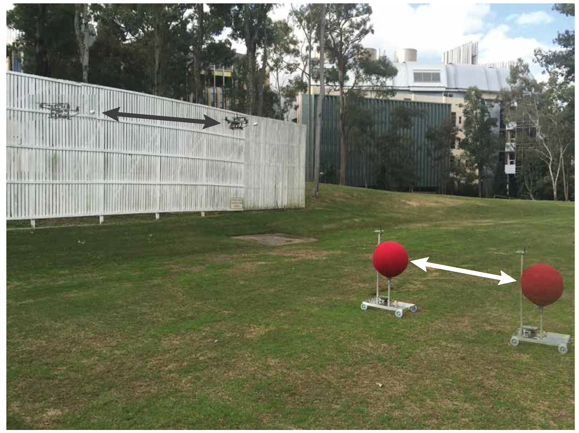
5. Guidance for Pursuit and Interception

In the field of robotics, interception is often characterised by military applications such as a drone neutralising a target. However, there are numerous applications in the civil environment as well, including target following, target inspection, docking, and search and rescue. Indeed, these applications are crucial for a complete UAS control suite.

5.1. Interception: An Engineering Approach to Pursue Ground Targets

This section will provide an engineering-based approach to pursue and intercept a ground target by using stereo information. Interception of ground targets has been demonstrated through the use of specialised fiducial marker-based targets [84], as well as the utilisation of additional sensors such as pressure sensors to measure altitude [87], or laser range finders [132] to determine the distance to the target. Although these methods have shown their capacity to intercept a ground target, the main limiting factor is that these methods require either a known target size and pattern, which in many cases would not be readily available; or the use of an additional height sensor (e.g., pressure, ultrasound, LiDAR, etc.) on top of the vision system, which adds an additional point of potential failure to the system.
The technique described in [133] utilises the imaging system, explained in Section 2.2, to detect a target and determines its position relative to the rotorcraft. To determine the relative position, and thus the relative velocity, the following steps are performed: (1) determine the direction to the target; (2) estimate the height above ground using stereo, which is independent of the presence of a target; and (3) geometrically compute the position of the target relative to the aircraft. Here stereo is particularly useful as it intrinsically provides the relative position between the rotorcraft and the target—to compute the distance to the target—Strydom, et al. [133] measures the aircraft’s HOG, which is then used to trigonometrically determine the target’s relative position (based on the azimuth and declination of the target); the attitude of the UAS is compensated for by using an AHRS, see Section 2.1. As a side note, by utilising the on-board panoramic vision system, the target can be detected in almost any direction. Using a PID controller, the distance between the target and the pursuer (UAS) is minimised, where the UAS velocity is proportional to the relative distance in the direction along the vector connecting the UAS and target positions.
To demonstrate the practicality of this approach, outdoor field experiments (Stereo-based UAS interception of a static target video available at: https://youtu.be/INi8OfsNIEA, Stereo-based UAS interception of a moving target video available at: https://youtu.be/XP_snIBXws4, similar to the schematic in Figure 16) were conducted by Strydom, et al. [133]. These results demonstrate that the approach outlined in [133] provides comparable results to current interception methods for a static or moving target, as outlined in Table 3. Note, that this is only a guide as only methods with quantitative results were compiled, and each method is tested under varying conditions and hardware configurations. There are, however, other methods such as [42] that also provide bio-inspired interception strategies.
Through experimentation it was clear that the main limiting factor of this method is the range at which the target can be accurately detected, and the range of the stereo measurements. Therefore, this method would be well suited to facilitate the interception of a ground target for the final stage of a pursuit or following strategy.

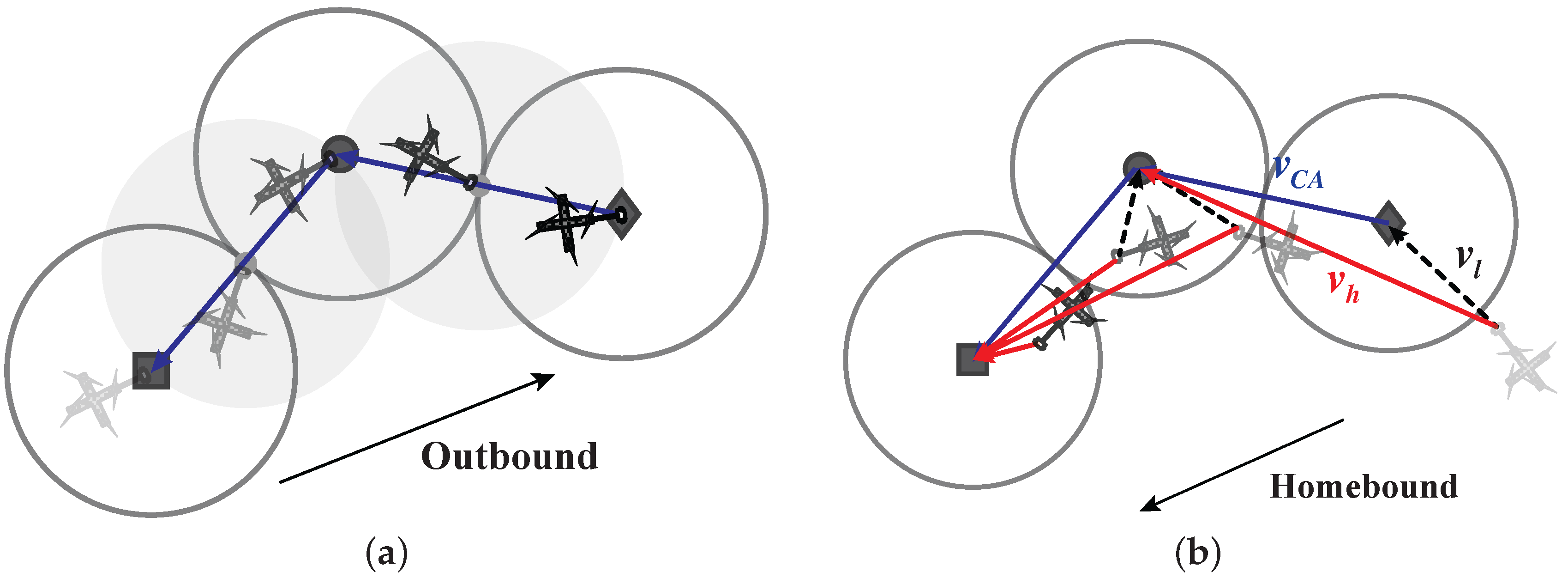
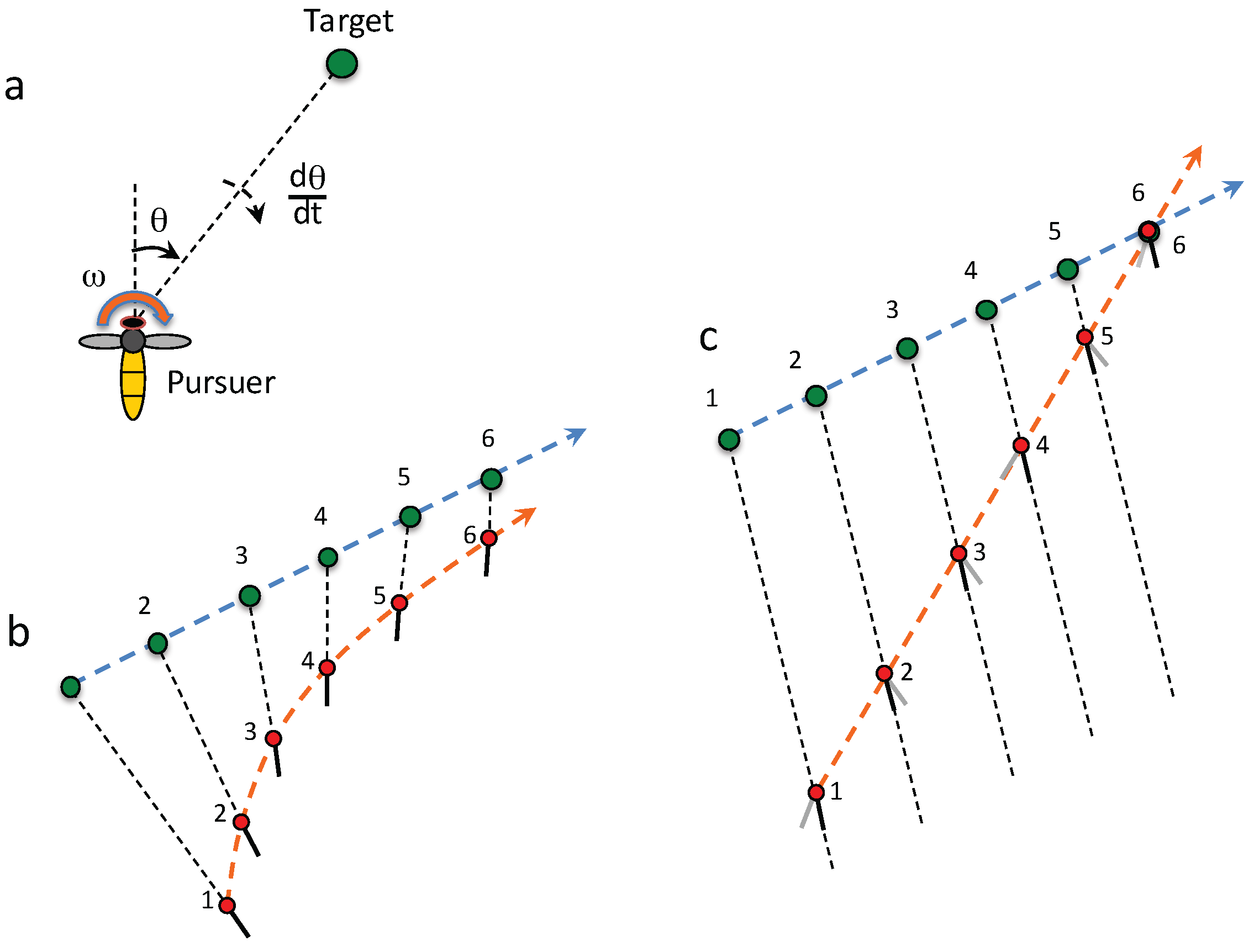
5.2. Interception: A Biological Approach

Many flying insects and birds seem to have evolved impressive strategies for pursuit and interception, overcoming some of the current engineering limitations such as the above stereo range, despite the fact that they possess limited sensing capacities. Thus, they are likely to provide important inspiration for the design of pursuit-control algorithms for UAS.
For many airborne animals, the ability to detect and pursue mates or prey, or to ward off intruders, is critical to survival of the individual as well as the species. In pioneering studies, References [137,138] used high-speed videography to study and model the behaviour of male flies pursuing other flies. They found that the chasing fly tracks the leading fly by means of a control system in which the turning (yaw) rate of the chaser is proportional to (i) the angle between the pursuer’s long axis and the angular bearing of the target, (the so-called “error angle”) and (ii) the rate of change of this error angle (Figure 17a). This feedback control system causes the pursuer to tend to point towards the target, without requiring specific knowledge of the object’s size or relative distance. While this kind of guidance strategy will eventually lead to capture if the target continues to move in a straight line and the pursuer is flying faster than the target, it is not necessarily the quickest way to intercept the target. This is because, even if the target is moving in a straight line at a constant speed, the pursuer’s trajectory will be a curve (Figure 17b).
Hoverflies overcome this problem by pre-computing a direct course of interception, based on information about the angular velocity of the target’s image in the pursuer’s eye at the time when the target is initially sighted [139]. Dragonflies seem to use a different, and perhaps more elegant interception strategy [20,140], in which they move in such a way that the absolute bearing of the target is held constant, as shown by the dashed lines in Figure 17c. If the target is moving in a straight line at a constant speed, then the pursuer’s trajectory (assuming that it also moves at a constant velocity) will also be a straight line (Figure 17c). This will ensure interception in the quickest possible time. This strategy of interception only requires preservation of the absolute bearing of the target. The orientation of the pursuer’s body during the chase does not matter, as shown by the grey lines in Figure 17c. If the target changes its direction or speed mid-stream, this will cause the pursuer to change its flight direction automatically, and set a new interception course that is optimal for the new condition. More recently, it has been demonstrated that constant-absolute-bearing interception of prey is also adopted by falcons [141] and echolocating bats [142].

5.3. Comparison of Pursuit and Constant-Bearing Interception Strategies

The first step to better understand these interception strategies in nature is to obtain a model that characterises the relationship between the visual input and the behavioural response. Although Land and Collett [137] provide a guidance law for the pursuit strategy (as described above—see (1) below), the sensorimotor delay in the system is not fully incorporated into their model. Strydom, et al. [143] introduce an additional term to this control law, which models the sensorimotor delay (the delay between sensing and action) observed in nature. This delay is modelled as a first-order low-pass filter with a time constant τ (see (2) below).
The resulting model [118] produces results similar to biological observations conducted by Land and Collett [137], providing intriguing evidence that, at least in the housefly, the sensorimotor delay is compensated for by the control system. Thus, the complete model compensates for the sensorimotor delay by computing the required ratio of the proportional (P) and derivative (D) gains for the PD guidance law by Land and Collett [137], as shown in (3).
P ( s ) = P θ + D d θ d t
M ( s ) = P ( s ) ( 1 / τ ) + s
T F = D P / D + s ( 1 / τ ) + s
Equation (3) reduces to a pure gain controller if P/D is selected to be equal to 1/τ, where τ is the sensorimotor time constant. This is a particularly useful property, as only one of the gains (P or D) has to be tuned to compensate for the sensorimotor delay, rather than both.

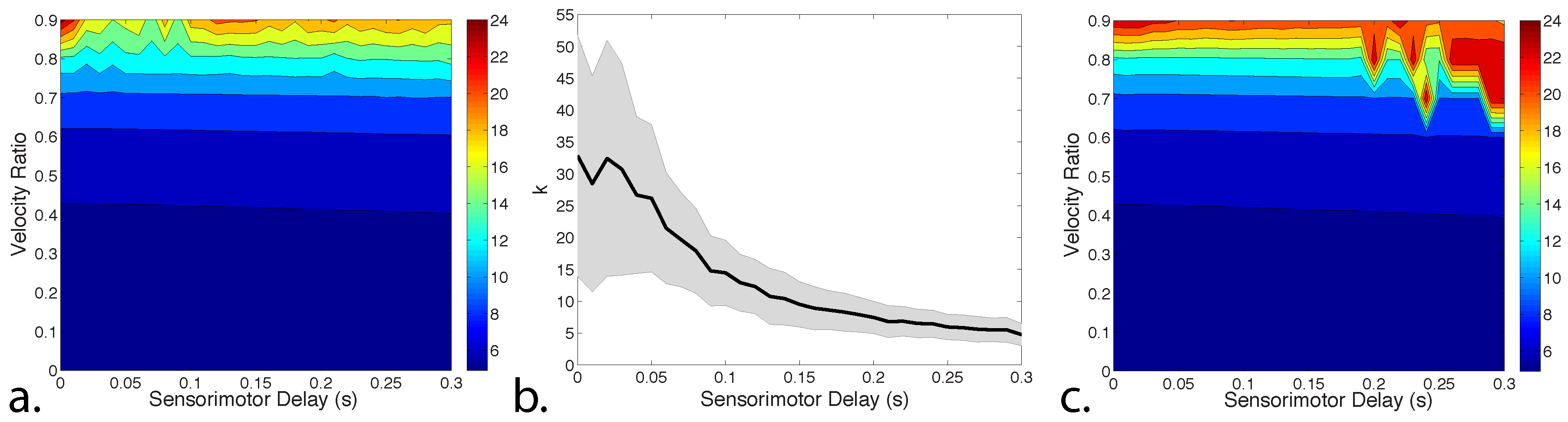
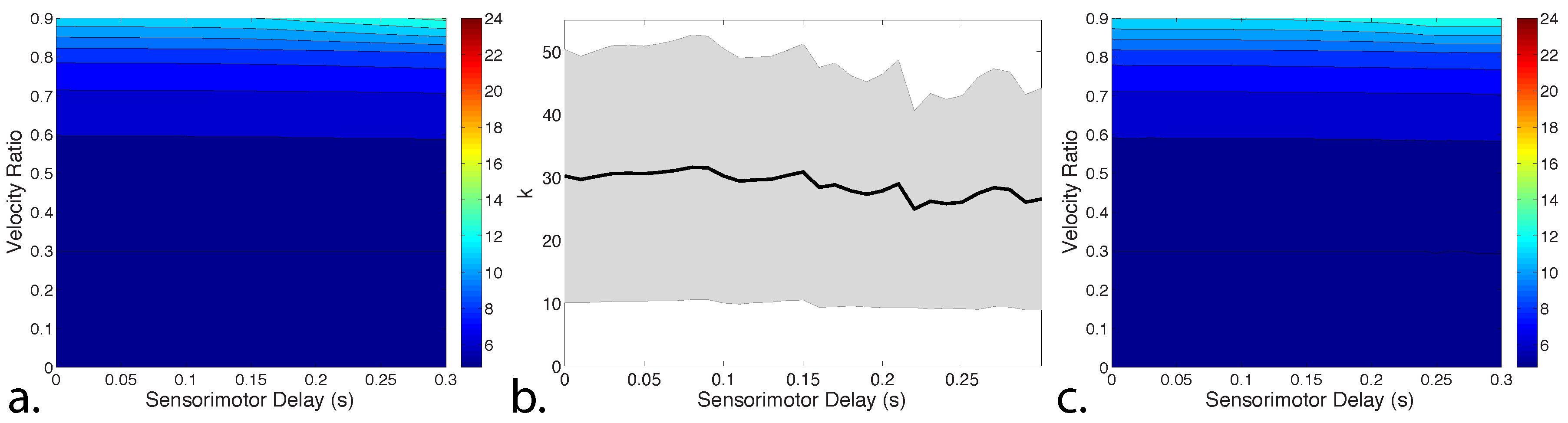
5.3.1. Evaluation of Pursuit and Interception Performance as a Function of Sensorimotor Delay

To provide a comparison between the constant bearing and pursuit strategies, Strydom, et al. [143] investigated both strategies modelled by the PD control law (by Land and Collett [137]) with the additional first-order lead lag filter to compensate for sensorimotor delay, as described in (3) above. The constant bearing and pursuit techniques were tested under the same initial conditions in simulation (e.g., initial target and pursuer positions and velocities). The key assumptions in the work by Strydom, et al. [143] are that the target moves with constant velocity, and that the pursuer’s velocity is greater than the target velocity.
In the scenario where the target is moving at constant velocity, the P gain was optimised for a range of sensorimotor delays and velocity ratios; the velocity ratio is the target speed divided by the pursuer speed. Only the P gain was optimised as the sensorimotor delay was compensated through the ratio of P and D in (3). It is demonstrated by Strydom, et al. [143] that the constant bearing strategy outperforms the pursuit strategy, as measured by the time taken for the pursuer to intercept the target. This is shown in Figure 18a and Figure 19a, which demonstrate that the constant bearing strategy provides a quicker interception time when the P gain is optimised for every velocity ratio (between 0 and 0.9) and sensorimotor delay (from 0 to 0.3 s) combination.
It was also found that rather than optimising P for every possible velocity ratio and sensorimotor delay, a mean P value over the range of velocity ratios values, as illustrated by Figure 18b and Figure 19b, can be used with near optimal performance for a particular sensorimotor delay, as shown in Figure 18c and Figure 19c. The changing value of P in Figure 18b, compared to the approximately constant value of P in Figure 19b, is an indication that the constant bearing strategy is more robust to variations in the velocity ratio and sensorimotor delays.
The main findings in [143] are that: (1) a controller consisting of a first order high-pass filter satisfactorily compensates for the sensorimotor delay in real biological control systems; (2) it is sufficient to use a single value of P for a particular sensorimotor delay, rather than optimise the P value for each velocity ratio; (3) the pursuit control law in [137] can also be used for constant bearing interception; and (4) in the scenario tested the constant bearing approach outperforms the pursuit strategy, measured by mean time to interception when optimising for every velocity ratio and sensorimotor delay combination, and also when using a single, optimised P gain.
Although the constant bearing strategy significantly outperforms the simple pursuit strategy, there may be advantages to using a pursuit strategy, for example, before starting a constant bearing approach or during the final moments before interception. Another situation where the pursuit strategy may be preferable (especially in robotics) is when the vision system has a limited field of view, thus requiring the target to be positioned close to the frontal direction of the pursuer.

5.3.2. Pursuit and Constant Bearing Interception in the Context of Robotics

Although not specifically designed for interception, there are other more engineering-based approaches that can be used for pursuit and interception. Examples include a Linear Quadratic Regulator (LQR), which may include sensorimotor delay as a part of the optimising objective function [144]. In general, however, LQR is used to optimise a number of parameters where individual gains would need to be re-adjusted for each sensorimotor delay. Another engineering technique is the well known Model Predictive Control (MPC), which is in affect a finite optimisation of a plant model [145]. MPC is known to provide high accuracy control, however, its main limitation is that an accurate dynamics model is often required, which is not always available.
One of the benefits of the model presented in [143] is the ability to simplify the tuning process of a robot’s controller for target interception through the use of bio-inspired principles. The tuning process is simplified by adjusting the ratio of (P/D) in the proportional controller to match the time constant of the low-pass filter that characterises the sensorimotor delay, thus requiring tuning of only one parameter in the PD controller. In the case of a rotorcraft UAS intercepting a target—for example, as described in the Section 5.1—the commanded flight direction that would be fed into the controller is computed by using a vision-based system to regulate the rotorcraft’s state through a PD controller.
As mentioned earlier, vision-based solutions can also provide challenging control problems for systems in which the computational load for visual processing, and therefore the sensorimotor delay can vary from moment to moment depending on the task currently being addressed: e.g., navigation, target detection, classification, tracking, or interception. The method proposed by Strydom, et al. [143] provides a means by which such varying sensorimotor delays could be compensated for in real time by an adaptive controller that uses a task-dependent look-up table to update the control relevant gains.
Finally, a key benefit of the bio-inspired approach to pursuit and constant bearing interception is that no prior information is required about the object (e.g., size, shape, etc.) or its relative position and velocity. By using only information about the observed direction, an object can be pursued by a robot (e.g., UAS) using either (or a combination) of the pursuit and constant bearing strategies.

6. Conclusions

The purpose of this paper is to provide a brief overview of bio-inspired principles to guidance and navigation, to facilitate the development of more autonomous UAS. Additionally, we provide a review of the key limitations of the current state-of-the-art in UAS. The potential advantages of biologically inspired techniques include navigation in cluttered GPS-denied environments, awareness of surrounding objects, and guidance strategies for the pursuit and interception of moving targets.
It is clear that animals, in particular insects, have demonstrated that simple vision-based approaches can be used to overcome many of these limitations. Indeed, insects manage perfectly well without external aids such as GPS, and although GPS provides useful position information, it does not provide information about the location of the next obstacle (unless a digital terrain map is also used). Vision, apart from being easy to miniaturise, has the added advantage that it involves the use of a multi-purpose sensor that offers a cost effective solution not just for navigation, but also for a number of other tasks in the domain of short-range guidance such as obstacle avoidance, altitude control and landing. Although many of these biologically inspired mechanisms and algorithms may or may not mimic nature in a literal sense, they adopt useful principles from animals to conduct tasks more efficiently.
It is shown that robust navigation can be achieved by the use of a panoramic imaging sensor in conjunction with biologically inspired guidance algorithms. We provide an overview of an optic flow technique for the estimation of the change in the rotorcraft state (e.g., position and velocity) from one frame to another. This method is capable of providing accurate information about the state of the aircraft for short-term flights, using visual odometry. However, the accuracy of the result decreases with increasing flight times and distances, due to the cumulative effect of noise. We show that a solution to this problem is to use sparse visual snapshots along selected waypoints, to achieve drift-free local and long-range homing. The main drawback of the current vision-based methods is the requirement of an AHRS (or IMU) to determine the orientation of the aircraft. We show, however, that vision can also be used to estimate aircraft attitude, thus paving the way for a navigation system that relies purely on vision.
Vision can be used not only for navigation, but also to gather situational awareness of the surrounding environment. An important requirement in the context of situational awareness is the ability to distinguish between moving and stationary objects. We have discussed a number of approaches to this challenging task. Notably, the epipolar constraint technique and the Triangle Closure Method (coined TCM), that can be implemented in the vision system of a UAS to reliably detect moving objects in the environment, and activate a sense-and-act response.
Once an object is deemed to be moving, action can be taken either to avoid it, or to pursue and intercept it. In this paper we focus on the latter manoeuvre. It is shown that biologically inspired strategies (e.g., pursuit and constant bearing) can be successfully used for target interception even in the face of large sensorimotor delays. The comparison of the pursuit and constant bearing strategies provides valuable insights into the differences in their performance. It is shown that a simple model for the sensorimotor delay as observed in nature can be utilised to effectively compensate for the delay and can be used to easily tune the control system. Finally, a stereo-based interception strategy is developed for the robust pursuit and interception (or following) of a ground-based target in an outdoor environment.
Table 4 provides a brief summary of the tasks that we have addressed in this review and the biologically inspired techniques that have been used to achieve them. It is clear that bio-inspired principles and vision-based techniques could hold the key for a UAS with greater autonomy. The combination of the sensing, navigation and guidance capacities discussed in this paper provide a stepping-stone for the development of more intelligent unmanned aerial systems, with a variety of applications ranging from guidance of flight in urban environments through to planetary exploration.

Acknowledgments

The research described here was supported partly by Boeing Defence Australia Grant SMP-BRT-11-044, ARC Linkage Grant LP130100483, ARC Discovery Grant DP140100896, a Queensland Premier’s Fellowship, and an ARC Distinguished Outstanding Researcher Award (DP140100914).

Author Contributions

Reuben Strydom contributed to Section 1, Section 2, Section 3 (Section 3.1, Section 3.2.2 and Section 3.3), Section 4 and Section 5. Aymeric Denuelle contributed to Section 3.2. Mandyam V. Srinivasan contributed to the biological research described in Section 2, Section 3, Section 4, Section 5 and to Section 3.1.2. All authors contributed to the writing of the manuscript.

Conflicts of Interest

The authors declare no conflict of interest.

References

  1. Gibbs, Y. Global Hawk—Performance and Specifications. Available online: http://www.nasa.gov/centers/armstrong/aircraft/GlobalHawk/performance.html (accessed on 9 June 2016).
  2. Golightly, G. Boeing’s Concept Exploration Pioneers New UAV Development with the Hummingbird and the Maverick. Available online: http://www.boeing.com/news/frontiers/archive/2004/december/tssf04.html (accessed on 9 June 2016).
  3. MQ-1B Predator. Available online: http://www.af.mil/AboutUs/FactSheets/Display/tabid/224/Article/104469/mq-1b-predator.aspx (accessed on 9 June 2016).
  4. Insitu. SCANEAGLE; Technical Report; Insitu: Washington, DC, USA, 2016. [Google Scholar]
  5. AeroVironment. Raven; Technical Report; AeroVironment: Monrovia, CA, USA, 2016. [Google Scholar]
  6. AirRobot. AIRROBOT; Technical Report; AirRobot: Arnsberg, Germany, 2007. [Google Scholar]
  7. DJI. Available online: http://www.dji.com/product/phantom-3-pro/info (accessed on 9 June 2016).
  8. Thrun, S.; Leonard, J.J. Simultaneous localization and mapping. In Springer Handbook of Robotics; Springer: Berlin, Germany; Heidelberg, Germany, 2008; pp. 871–889. [Google Scholar]
  9. Clark, S.; Durrant-Whyte, H. Autonomous land vehicle navigation using millimeter wave radar. In Proceedings of the 1998 IEEE International Conference on Robotics and Automation, Leuven, Belgium, 16–20 May 1998; Volume 4, pp. 3697–3702.
  10. Clark, S.; Dissanayake, G. Simultaneous localisation and map building using millimetre wave radar to extract natural features. In Proceedings of the 1999 IEEE International Conference on Robotics and Automation, Detroit, MI, USA, 10–15 May 1999; Volume 2, pp. 1316–1321.
  11. Jose, E.; Adams, M.D. Millimetre wave radar spectra simulation and interpretation for outdoor slam. In Proceedings of the 2004 IEEE International Conference on Robotics and Automation, ICRA’04, New Orleans, LA, USA, 26 April–1 May 2004; Volume 2, pp. 1321–1326.
  12. Clothier, R.; Frousheger, D.; Wilson, M.; Grant, I. The smart skies project: Enabling technologies for future airspace environments. In Proceedings of the 28th Congress of the International Council of the Aeronautical Sciences, International Council of the Aeronautical Sciences, Brisbane, Australia; 2012; pp. 1–12. [Google Scholar]
  13. Wilson, M. Ground-Based Sense and Avoid Support for Unmanned Aircraft Systems. In Proceedings of the Congress of the International Council of the Aeronautical Sciences (ICAS), Brisbane, Australia, 23–28 September 2012.
  14. Korn, B.; Edinger, C. UAS in civil airspace: Demonstrating “sense and avoid” capabilities in flight trials. In Proceedings of the 2008 IEEE/AIAA 27th Digital Avionics Systems Conference, St. Paul, MN, USA, 26–30 October 2008; pp. 4.D.1-1–4.D.1-7.
  15. Viquerat, A.; Blackhall, L.; Reid, A.; Sukkarieh, S.; Brooker, G. Reactive collision avoidance for unmanned aerial vehicles using doppler radar. In Field and Service Robotics; Springer: Berlin, Germany; Heidelberg, Germany, 2008; pp. 245–254. [Google Scholar]
  16. Australian Transport Safety Bureau (ATSB). Review of Midair Collisions Involving General Aviation Aircraft in Australia between 1961 and 2003; ATSB: Canberra, Australia, 2004.
  17. Hayhurst, K.J.; Maddalon, J.M.; Miner, P.S.; DeWalt, M.P.; McCormick, G.F. Unmanned aircraft hazards and their implications for regulation. In Proceedings of the 2006 IEEE/AIAA 25th Digital Avionics Systems Conference, Portland, OR, USA, 15–19 October 2006; pp. 1–12.
  18. Srinivasan, M.V. Honeybees as a model for the study of visually guided flight, navigation, and biologically inspired robotics. Physiol. Rev. 2011, 91, 413–460. [Google Scholar] [CrossRef] [PubMed]
  19. Srinivasan, M.V. Visual control of navigation in insects and its relevance for robotics. Curr. Opin. Neurobiol. 2011, 21, 535–543. [Google Scholar] [CrossRef] [PubMed]
  20. Mischiati, M.; Lin, H.T.; Herold, P.; Imler, E.; Olberg, R.; Leonardo, A. Internal models direct dragonfly interception steering. Nature 2015, 517, 333–338. [Google Scholar] [CrossRef] [PubMed]
  21. Franceschini, N. Small brains, smart machines: From fly vision to robot vision and back again. Proc. IEEE 2014, 102, 751–781. [Google Scholar] [CrossRef]
  22. Roubieu, F.L.; Serres, J.R.; Colonnier, F.; Franceschini, N.; Viollet, S.; Ruffier, F. A biomimetic vision-based hovercraft accounts for bees’ complex behaviour in various corridors. Bioinspir. Biomim. 2014, 9, 036003. [Google Scholar] [CrossRef] [PubMed]
  23. Ruffier, F.; Franceschini, N. Optic flow regulation: The key to aircraft automatic guidance. Robot. Auton. Syst. 2005, 50, 177–194. [Google Scholar] [CrossRef]
  24. Floreano, D.; Zufferey, J.C.; Srinivasan, M.V.; Ellington, C. Flying Insects and Robots; Springer: Berlin, Germany; Heidelberg, Germany, 2009. [Google Scholar]
  25. Srinivasan, M.V.; Moore, R.J.; Thurrowgood, S.; Soccol, D.; Bland, D.; Knight, M. Vision and Navigation in Insects, and Applications to Aircraft Guidance; The MIT Press: Cambridge, MA, USA, 2014. [Google Scholar]
  26. Coombs, D.; Roberts, K. ’Bee-Bot’: Using Peripheral Optical Flow to Avoid Obstacles. In Proc. SPIE 1825, Proceedings of Intelligent Robots and Computer Vision XI: Algorithms, Techniques, and Active Vision, Boston, MA, USA, 15 November 1992; pp. 714–721.
  27. Santos-Victor, J.; Sandini, G.; Curotto, F.; Garibaldi, S. Divergent stereo in autonomous navigation: From bees to robots. Int. J. Comput. Vis. 1995, 14, 159–177. [Google Scholar] [CrossRef]
  28. Weber, K.; Venkatesh, S.; Srinivasan, M.V. Insect inspired behaviours for the autonomous control of mobile robots. In Proceedings of the 13th International Conference on Pattern Recognition, Vienna, Austria, 25–29 August 1996; Volume 1, pp. 156–160.
  29. Conroy, J.; Gremillion, G.; Ranganathan, B.; Humbert, J.S. Implementation of wide-field integration of optic flow for autonomous quadrotor navigation. Auton. Robot. 2009, 27, 189–198. [Google Scholar] [CrossRef]
  30. Sabo, C.M.; Cope, A.; Gurney, K.; Vasilaki, E.; Marshall, J. Bio-Inspired Visual Navigation for a Quadcopter using Optic Flow. In AIAA Infotech @ Aerospace; American Institute of Aeronautics and Astronautics: Reston, VA, USA, 2016; Volume 404, pp. 1–14. [Google Scholar]
  31. Zufferey, J.C.; Floreano, D. Fly-inspired visual steering of an ultralight indoor aircraft. IEEE Trans. Robot. 2006, 22, 137–146. [Google Scholar] [CrossRef]
  32. Garratt, M.A.; Chahl, J.S. Vision-based terrain following for an unmanned rotorcraft. J. Field Robot. 2008, 25, 284–301. [Google Scholar] [CrossRef]
  33. Moore, R.J.; Thurrowgood, S.; Bland, D.; Soccol, D.; Srinivasan, M.V. UAV altitude and attitude stabilisation using a coaxial stereo vision system. In Proceedings of the 2010 IEEE International Conference on Robotics and Automation (ICRA), Anchorage, AK, USA, 3–7 May 2010; pp. 29–34.
  34. Cornall, T.; Egan, G.; Price, A. Aircraft attitude estimation from horizon video. Electron. Lett. 2006, 42, 744–745. [Google Scholar] [CrossRef]
  35. Horiuchi, T.K. A low-power visual-horizon estimation chip. IEEE Trans. Circuits Syst. I Regul. Pap. 2009, 56, 1566–1575. [Google Scholar] [CrossRef]
  36. Moore, R.; Thurrowgood, S.; Bland, D.; Soccol, D.; Srinivasan, M.V. A fast and adaptive method for estimating UAV attitude from the visual horizon. In Proceedings of the 2011 IEEE/RSJ International Conference on Intelligent Robots and Systems, San Francisco, CA, USA, 25–30 September 2011.
  37. Jouir, T.; Strydom, R.; Srinivasan, M.V. A 3D sky compass to achieve robust estimation of UAV attitude. In Proceedings of the Australasian Conference on Robotics and Automation, Canberra, Australia, 2–4 December 2015.
  38. Zhang, Z.; Xie, P.; Ma, O. Bio-inspired trajectory generation for UAV perching. In Proceedings of the 2013 IEEE/ASME International Conference on Advanced Intelligent Mechatronics (AIM), Wollongong, Australia, 9–12 July 2013; pp. 997–1002.
  39. Zhang, Z.; Zhang, S.; Xie, P.; Ma, O. Bioinspired 4D trajectory generation for a UAS rapid point-to-point movement. J. Bionic Eng. 2014, 11, 72–81. [Google Scholar] [CrossRef]
  40. Zhang, Z.; Xie, P.; Ma, O. Bio-inspired trajectory generation for UAV perching movement based on tau theory. Int. J. Adv. Robot. Syst. 2014, 11, 141. [Google Scholar] [CrossRef]
  41. Xie, P.; Ma, O.; Zhang, Z. A bio-inspired approach for UAV landing and perching. In Proceedings of the AIAA GNC, Boston, MA, USA, 19–22 August 2013; Volume 13.
  42. Kendoul, F. Four-dimensional guidance and control of movement using time-to-contact: Application to automated docking and landing of unmanned rotorcraft systems. Int. J. Robot. Res. 2014, 33, 237–267. [Google Scholar] [CrossRef]
  43. Beyeler, A.; Zufferey, J.C.; Floreano, D. optiPilot: Control of take-off and landing using optic flow. In Proceedings of the 2009 European Micro Air Vehicle conference and competition (EMAV 09), Delft, The Netherland, 14–17 September 2009.
  44. Herissé, B.; Hamel, T.; Mahony, R.; Russotto, F.X. Landing a VTOL unmanned aerial vehicle on a moving platform using optical flow. IEEE Trans. Robot. 2012, 28, 77–89. [Google Scholar] [CrossRef]
  45. Kendoul, F.; Fantoni, I.; Nonami, K. Optic flow-based vision system for autonomous 3D localization and control of small aerial vehicles. Robot. Auton. Syst. 2009, 57, 591–602. [Google Scholar] [CrossRef]
  46. Thurrowgood, S.; Moore, R.J.; Soccol, D.; Knight, M.; Srinivasan, M.V. A Biologically Inspired, Vision-based Guidance System for Automatic Landing of a Fixed-wing Aircraft. J. Field Robot. 2014, 31, 699–727. [Google Scholar] [CrossRef]
  47. Chahl, J. Unmanned Aerial Systems (UAS) Research Opportunities. Aerospace 2015, 2, 189–202. [Google Scholar] [CrossRef]
  48. Duan, H.; Li, P. Bio-Inspired Computation in Unmanned Aerial Vehicles; Springer: Berlin, Germany; Heidelberg, Germany, 2014. [Google Scholar]
  49. Evangelista, C.; Kraft, P.; Dacke, M.; Reinhard, J.; Srinivasan, M.V. The moment before touchdown: Landing manoeuvres of the honeybee Apis mellifera. J. Exp. Biol. 2010, 213, 262–270. [Google Scholar] [CrossRef] [PubMed]
  50. Kannala, J.; Brandt, S.S. A generic camera model and calibration method for conventional, wide-angle, and fish-eye lenses. IEEE Trans. Pattern Anal. Mach. Intell. 2006, 28, 1335–1340. [Google Scholar] [CrossRef] [PubMed]
  51. Goodman, L. Form and Function in the Honey Bee; International Bee Research Association: Bristol, UK, 2003. [Google Scholar]
  52. Koenderink, J.J.; van Doorn, A.J. Facts on optic flow. Biol. Cybern. 1987, 56, 247–254. [Google Scholar] [CrossRef] [PubMed]
  53. Krapp, H.G.; Hengstenberg, R. Estimation of self-motion by optic flow processing in single visual interneurons. Nature 1996, 384, 463–466. [Google Scholar] [CrossRef] [PubMed]
  54. Krapp, H.G.; Hengstenberg, B.; Hengstenberg, R. Dendritic structure and receptive-field organization of optic flow processing interneurons in the fly. J. Neurophysiol. 1998, 79, 1902–1917. [Google Scholar] [PubMed]
  55. Lucas, B.D.; Kanade, T. An iterative image registration technique with an application to stereo vision. In Proceedings of the IJCAI, Vancouver, BC, Canada, 24–28 August 1981; Volume 81, pp. 674–679.
  56. Horn, B.K.; Schunck, B.G. Determining optical flow. Artif. Intell. 1981, 71, 319–331. [Google Scholar] [CrossRef]
  57. Expert, F.; Ruffier, F. Flying over uneven moving terrain based on optic-flow cues without any need for reference frames or accelerometers. Bioinspir. Biomim. 2015, 10, 026003. [Google Scholar] [CrossRef] [PubMed]
  58. Maimone, M.; Cheng, Y.; Matthies, L. Two years of visual odometry on the mars exploration rovers. J. Field Robot. 2007, 24, 169–186. [Google Scholar] [CrossRef]
  59. Strydom, R.; Thurrowgood, S.; Srinivasan, M.V. Visual Odometry: Autonomous UAV Navigation using Optic Flow and Stereo. In Proceedings of the Australasian Conference on Robotics and Automation, Melbourne, Australia, 2–4 December 2014.
  60. Von Frisch, K. The Dance Language and Orientation of Bees; Harvard University Press: Cambridge, MA, USA, 1967. [Google Scholar]
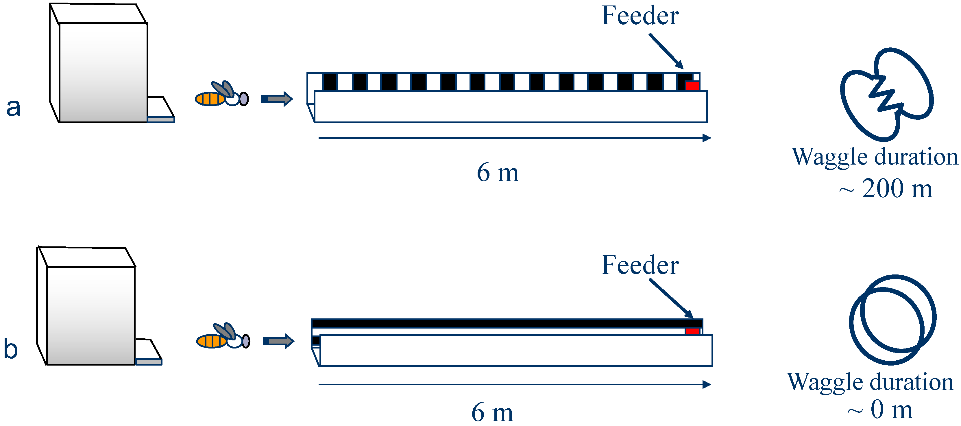
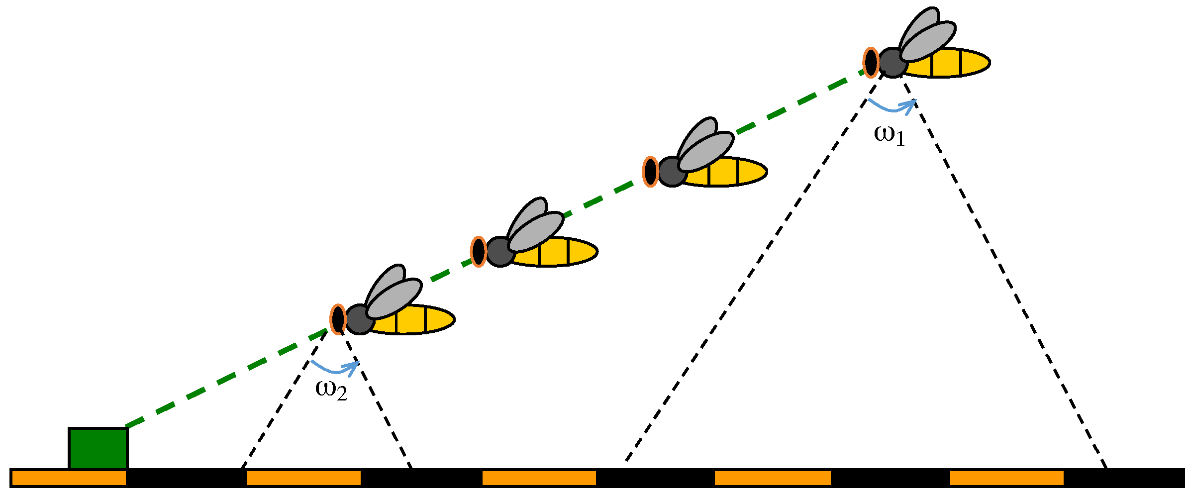
  61. Srinivasan, M.V.; Zhang, S.W.; Altwein, M.; Tautz, J. Honeybee navigation: Nature and calibration of the “odometer”. Science 2000, 287, 851–853. [Google Scholar] [CrossRef] [PubMed]
  62. Esch, H.E.; Zhang, S.W.; Srinivasan, M.V.; Tautz, J. Honeybee dances communicate distances measured by optic flow. Nature 2001, 411, 581–583. [Google Scholar] [CrossRef] [PubMed]
  63. Sünderhauf, N.; Protzel, P. Stereo Odometry—A Review of Approaches; Technical Report; Chemnitz University of Technology: Chemnitz, Germany, 2007. [Google Scholar]
  64. Alismail, H.; Browning, B.; Dias, M.B. Evaluating pose estimation methods for stereo visual odometry on robots. In Proceedings of the 2010 11th International Conference on Intelligent Autonomous Systems (IAS-11), Ottawa, ON, Canada, 30 August–1 September 2010.
  65. Badino, H.; Yamamoto, A.; Kanade, T. Visual odometry by multi-frame feature integration. In Proceedings of the IEEE International Conference on Computer Vision Workshops, Sydney, Australia, 2–8 December 2013; pp. 222–229.
  66. Nistér, D.; Naroditsky, O.; Bergen, J. Visual odometry. In Proceedings of the 2004 IEEE Computer Society Conference on Computer Vision and Pattern Recognition, CVPR 2004, Washington, DC, USA, 27 June–2 July 2004; Volume 1, pp. I-652–I-659.
  67. Nistér, D.; Naroditsky, O.; Bergen, J. Visual odometry for ground vehicle applications. J. Field Robot. 2006, 23, 3–20. [Google Scholar] [CrossRef]
  68. Warren, M.; Corke, P.; Upcroft, B. Long-range stereo visual odometry for extended altitude flight of unmanned aerial vehicles. Int. J. Robot. Res. 2016, 35, 381–403. [Google Scholar] [CrossRef]
  69. Caballero, F.; Merino, L.; Ferruz, J.; Ollero, A. Vision-based odometry and SLAM for medium and high altitude flying UAVs. J. Intell. Robot. Syst. 2009, 54, 137–161. [Google Scholar] [CrossRef]
  70. Scaramuzza, D.; Siegwart, R. Appearance-guided monocular omnidirectional visual odometry for outdoor ground vehicles. IEEE Trans. Robot. 2008, 24, 1015–1026. [Google Scholar] [CrossRef]
  71. More, V.; Kumar, H.; Kaingade, S.; Gaidhani, P.; Gupta, N. Visual odometry using optic flow for Unmanned Aerial Vehicles. In Proceedings of the 2015 International Conference on Cognitive Computing and Information Processing (CCIP), Noida, India, 3–4 March 2015; pp. 1–6.
  72. Corke, P.; Strelow, D.; Singh, S. Omnidirectional visual odometry for a planetary rover. In Proceedings of the 2004 IEEE/RSJ International Conference on Intelligent Robots and Systems, 2004 (IROS 2004), Sendai, Japan, 28 September–2 October 2004; Volume 4, pp. 4007–4012.
  73. Campbell, J.; Sukthankar, R.; Nourbakhsh, I. Techniques for evaluating optical flow for visual odometry in extreme terrain. In Proceedings of the 2004 IEEE/RSJ International Conference on Intelligent Robots and Systems, 2004 (IROS 2004), Sendai, Japan, 28 September–2 October 2004; Volume 4, pp. 3704–3711.
  74. Scaramuzza, D.; Fraundorfer, F. Visual Odometry. Part 1: The first 30 years and fundamentals. IEEE Robot. Autom. Mag. 2011, 18, 80–92. [Google Scholar] [CrossRef]
  75. Olson, C.F.; Matthies, L.H.; Schoppers, M.; Maimone, M.W. Robust stereo ego-motion for long distance navigation. In Proceedings of the IEEE Conference on Computer Vision and Pattern Recognition, Hilton Head Island, SC, USA, 13–15 June 2000; Volume 2, pp. 453–458.
  76. Tardif, J.P.; Pavlidis, Y.; Daniilidis, K. Monocular visual odometry in urban environments using an omnidirectional camera. In Proceedings of the 2008 IEEE/RSJ International Conference on Intelligent Robots and Systems, Nice, France, 22–26 September 2008; pp. 2531–2538.
  77. Heng, L.; Honegger, D.; Lee, G.H.; Meier, L.; Tanskanen, P.; Fraundorfer, F.; Pollefeys, M. Autonomous Visual Mapping and Exploration with a Micro Aerial Vehicle. J. Field Robot. 2014, 31, 654–675. [Google Scholar] [CrossRef]
  78. Nourani-Vatani, N.; Borges, P.V.K. Correlation-based visual odometry for ground vehicles. J. Field Robot. 2011, 28, 742–768. [Google Scholar] [CrossRef]
  79. Lemaire, T.; Berger, C.; Jung, I.K.; Lacroix, S. Vision-based slam: Stereo and monocular approaches. Int. J. Comput. Vis. 2007, 74, 343–364. [Google Scholar] [CrossRef]
  80. Salazar-Cruz, S.; Escareno, J.; Lara, D.; Lozano, R. Embedded control system for a four-rotor UAV. Int. J. Adapt. Control Signal Process. 2007, 21, 189–204. [Google Scholar] [CrossRef]
  81. Kendoul, F.; Lara, D.; Fantoni, I.; Lozano, R. Real-time nonlinear embedded control for an autonomous quadrotor helicopter. J. Guid. Control Dyn. 2007, 30, 1049–1061. [Google Scholar] [CrossRef]
  82. Mori, R.; Kubo, T.; Kinoshita, T. Vision-based hovering control of a small-scale unmanned helicopter. In Proceedings of the International Joint Conference SICE-ICASE, Busan, Korean, 18–21 October 2006; pp. 1274–1278.
  83. Guenard, N.; Hamel, T.; Mahony, R. A practical visual servo control for an unmanned aerial vehicle. IEEE Trans. Robot. 2008, 24, 331–340. [Google Scholar] [CrossRef] [Green Version]
  84. Lange, S.; Sunderhauf, N.; Protzel, P. A vision based onboard approach for landing and position control of an autonomous multirotor UAV in GPS-denied environments. In Proceedings of the International Conference on Advanced Robotics, 2009, ICAR 2009, Munich, Germany, 22–26 June 2009.
  85. Yang, S.; Scherer, S.A.; Zell, A. An onboard monocular vision system for autonomous takeoff, hovering and landing of a micro aerial vehicle. J. Intell. Robot. Syst. 2013, 69, 499–515. [Google Scholar] [CrossRef]
  86. Masselli, A.; Zell, A. A novel marker based tracking method for position and attitude control of MAVs. In Proceedings of the International Micro Air Vehicle Conference and Flight Competition (IMAV), Braunschweig, Germany, 3–6 July 2012.
  87. Azrad, S.; Kendoul, F.; Nonami, K. Visual servoing of quadrotor micro-air vehicle using color-based tracking algorithm. J. Syst. Des. Dyn. 2010, 4, 255–268. [Google Scholar] [CrossRef]
  88. Achtelik, M.; Achtelik, M.; Weiss, S.; Siegwart, R. Onboard IMU and monocular vision based control for MAVs in unknown in-and outdoor environments. In Proceedings of the 2011 IEEE International Conference on Robotics and Automation (ICRA), Shanghai, China, 9–13 May 2011; pp. 3056–3063.
  89. Shen, S.; Mulgaonkar, Y.; Michael, N.; Kumar, V. Vision-based state estimation for autonomous rotorcraft mavs in complex environments. In Proceedings of the 2013 IEEE International Conference on Robotics and Automation (ICRA), Karlsruhe, Germany, 6–10 May 2013; pp. 1758–1764.
  90. Zeil, J.; Hofmann, M.I.; Chahl, J.S. Catchment areas of panoramic snapshots in outdoor scenes. JOSA A 2003, 20, 450–469. [Google Scholar] [CrossRef] [PubMed]
  91. Denuelle, A.; Thurrowgood, S.; Kendoul, F.; Srinivasan, M.V. A view-based method for local homing of unmanned rotorcraft. In Proceedings of the 2015 6th International Conference on Automation, Robotics and Applications (ICARA), Queenstown, New Zealand, 17–19 February 2015; pp. 443–449.
  92. Denuelle, A.; Thurrowgood, S.; Strydom, R.; Kendoul, F.; Srinivasan, M.V. Biologically-inspired visual stabilization of a rotorcraft UAV in unknown outdoor environments. In Proceedings of the International Conference on Unmanned Aircraft Systems (ICUAS), Denver, CO, USA, 9–12 June 2015; pp. 1084–1093.
  93. Denuelle, A.; Strydom, R.; Srinivasan, M.V. Snapshot-based control of UAS hover in outdoor environments. In Proceedings of the 2015 IEEE International Conference on Robotics and Biomimetics (ROBIO), Zhuhai, China, 6–9 December 2015; pp. 1278–1284.
  94. Romero, H.; Salazar, S.; Lozano, R. Real-time stabilization of an eight-rotor UAV using optical flow. IEEE Trans. Robot. 2009, 25, 809–817. [Google Scholar] [CrossRef]
  95. Li, P.; Garratt, M.; Lambert, A.; Pickering, M.; Mitchell, J. Onboard hover control of a quadrotor using template matching and optic flow. In Proceedings of the International Conference on Image Processing, Computer Vision, and Pattern Recognition (IPCV). The Steering Committee of The World Congress in Computer Science, Computer Engineering and Applied Computing (WorldComp), Las Vegas, NV, USA, 22–25 July 2013; p. 1.
  96. Green, W.E.; Oh, P.Y.; Barrows, G. Flying insect inspired vision for autonomous aerial robot maneuvers in near-earth environments. In Proceedings of the 2004 IEEE International Conference on Robotics and Automation, New Orleans, LA, USA, 26 April–1 May 2004; Volume 3, pp. 2347–2352.
  97. Colonnier, F.; Manecy, A.; Juston, R.; Mallot, H.; Leitel, R.; Floreano, D.; Viollet, S. A small-scale hyperacute compound eye featuring active eye tremor: Application to visual stabilization, target tracking, and short-range odometry. Bioinspir. Biomim. 2015, 10, 026002. [Google Scholar] [CrossRef] [PubMed]
  98. Li, P.; Garratt, M.; Lambert, A. Monocular Snapshot-based Sensing and Control of Hover, Takeoff, and Landing for a Low-cost Quadrotor. J. Field Robot. 2015, 32, 984–1003. [Google Scholar] [CrossRef]
  99. Matsumoto, Y.; Inaba, M.; Inoue, H. Visual navigation using view-sequenced route representation. In Proceedings of the 1996 IEEE International Conference on Robotics and Automation, Minneapolis, MN, USA, 22–28 April 1996; Volume 1, pp. 83–88.
  100. Jones, S.D.; Andresen, C.; Crowley, J.L. Appearance based process for visual navigation. In Proceedings of the 1997 IEEE/RSJ International Conference on Intelligent Robots and Systems, Grenoble, France, 7–11 September 1997; Volume 2, pp. 551–557.
  101. Vardy, A. Long-range visual homing. In Proceedings of the 2006 IEEE International Conference on Robotics and Biomimetics, Kunming, China, 17–20 December 2006; pp. 220–226.
  102. Smith, L.; Philippides, A.; Graham, P.; Baddeley, B.; Husbands, P. Linked local navigation for visual route guidance. Adapt. Behav. 2007, 15, 257–271. [Google Scholar] [CrossRef]
  103. Labrosse, F. Short and long-range visual navigation using warped panoramic images. Robot. Auton. Syst. 2007, 55, 675–684. [Google Scholar] [CrossRef] [Green Version]
  104. Zhou, C.; Wei, Y.; Tan, T. Mobile robot self-localization based on global visual appearance features. In Proceedings of the 2003 IEEE International Conference on Robotics and Automation, Taipei, Taiwan, 14–19 September 2003; Volume 1, pp. 1271–1276.
  105. Argyros, A.A.; Bekris, K.E.; Orphanoudakis, S.C.; Kavraki, L.E. Robot homing by exploiting panoramic vision. Auton. Robot. 2005, 19, 7–25. [Google Scholar] [CrossRef]
  106. Courbon, J.; Mezouar, Y.; Guenard, N.; Martinet, P. Visual navigation of a quadrotor aerial vehicle. In Proceedings of the 2009 IEEE/RSJ International Conference on Intelligent Robots and Systems, St. Louis, MO, USA, 10–15 October 2009; pp. 5315–5320.
  107. Fu, Y.; Hsiang, T.R. A fast robot homing approach using sparse image waypoints. Image Vis. Comput. 2012, 30, 109–121. [Google Scholar] [CrossRef]
  108. Smith, L.; Philippides, A.; Husbands, P. Navigation in large-scale environments using an augmented model of visual homing. In From Animals to Animats 9; Springer: Berlin, Germany; Heidelberg, Germany, 2006; pp. 251–262. [Google Scholar]
  109. Chen, Z.; Birchfield, S.T. Qualitative vision-based mobile robot navigation. In Proceedings of the 2006 IEEE International Conference on Robotics and Automation, Orlando, FL, USA, 15–19 May 2006; pp. 2686–2692.
  110. Ohno, T.; Ohya, A.; Yuta, S.I. Autonomous navigation for mobile robots referring pre-recorded image sequence. In Proceedings of the 1996 IEEE/RSJ International Conference on Intelligent Robots and Systems, Osaka, Japan, 4–8 November 1996; Volume 2, pp. 672–679.
  111. Sagüés, C.; Guerrero, J.J. Visual correction for mobile robot homing. Robot. Auton. Syst. 2005, 50, 41–49. [Google Scholar] [CrossRef]
  112. Denuelle, A.; Srinivasan, M.V. Snapshot-based Navigation for the Guidance of UAS. In Proceedings of the Australasian Conference on Robotics and Automation, Canberra, Australia, 2–4 December 2015.
  113. Denuelle, A.; Srinivasan, M.V. A sparse snapshot-based navigation strategy for UAS guidance in natural environments. In Proceedings of the 2016 IEEE International Conference on Robotics and Automation (ICRA), Stockholm, Sweden, 16–21 May 2016; pp. 3455–3462.
  114. Rohac, J. Accelerometers and an aircraft attitude evaluation. In Proceedings of the IEEE Sensors, Irvine, CA, USA, 30 October–3 November 2005; p. 6.
  115. Thurrowgood, S.; Moore, R.J.; Bland, D.; Soccol, D.; Srinivasan, M.V. UAV attitude control using the visual horizon. In Proceedings of the Australasian Conference on Robotics and Automation, Brisbane, Australia, 1–3 December 2010.
  116. Lai, J.; Ford, J.J.; Mejias, L.; O’Shea, P. Characterization of Sky-region Morphological-temporal Airborne Collision Detection. J. Field Robot. 2013, 30, 171–193. [Google Scholar] [CrossRef]
  117. Nussberger, A.; Grabner, H.; Van Gool, L. Aerial object tracking from an airborne platform. In Proceedings of the 2014 International Conference on Unmanned Aircraft Systems (ICUAS), Orlando, FL, USA, 27–30 May 2014.
  118. Wenzel, K.E.; Rosset, P.; Zell, A. Low-cost visual tracking of a landing place and hovering flight control with a microcontroller. J. Intell. Robot. Syst. 2010, 57, 297. [Google Scholar] [CrossRef]
  119. Choi, J.H.; Lee, D.; Bang, H. Tracking an unknown moving target from UAV: Extracting and localizing an moving target with vision sensor based on optical flow. In Proceedings of the 2011 5th International Conference on Automation, Robotics and Applications (ICARA), Wellington, New Zealand, 6–8 December 2011.
  120. Pinto, A.M.; Costa, P.G.; Moreira, A.P. Introduction to Visual Motion Analysis for Mobile Robots. In CONTROLO’2014–Proceedings of the 11th Portuguese Conference on Automatic Control; Springer: Berlin, Germany; Heidelberg, Germany, 2015; pp. 545–554. [Google Scholar]
  121. Elhabian, S.Y.; El-Sayed, K.M.; Ahmed, S.H. Moving object detection in spatial domain using background removal techniques-state-of-art. Recent Pat. Comput. Sci. 2008, 1, 32–54. [Google Scholar] [CrossRef]
  122. Spagnolo, P.; Leo, M.; Distante, A. Moving object segmentation by background subtraction and temporal analysis. Image Vis. Comput. 2006, 24, 411–423. [Google Scholar] [CrossRef]
  123. Hayman, E.; Eklundh, J.O. Statistical background subtraction for a mobile observer. In Proceedings of the Ninth IEEE International Conference on Computer Vision, Nice, France, 13–16 October 2003; pp. 67–74.
  124. Sheikh, Y.; Javed, O.; Kanade, T. Background subtraction for freely moving cameras. In Proceedings of the 2009 IEEE 12th International Conference on Computer Vision, Kyoto, Japan, 29 Sptember–2 Octomber 2009; pp. 1219–1225.
  125. Kim, I.S.; Choi, H.S.; Yi, K.M.; Choi, J.Y.; Kong, S.G. Intelligent visual surveillance—A survey. Int. J. Control Autom. Syst. 2010, 8, 926–939. [Google Scholar] [CrossRef]
  126. Thakoor, N.; Gao, J.; Chen, H. Automatic object detection in video sequences with camera in motion. In Proceedings of the Advanced Concepts for Intelligent Vision Systems, Brussels, Belgium, 31 August–3 September 2004.
  127. Pinto, A.M.; Moreira, A.P.; Correia, M.V.; Costa, P.G. A flow-based motion perception technique for an autonomous robot system. J. Intell. Robot. Syst. 2014, 75, 475–492. [Google Scholar] [CrossRef]
  128. Strydom, R.; Thurrowgood, S.; Srinivasan, M.V. Airborne vision system for the detection of moving objects. In Proceedings of the Australasian Conference on Robotics and Automation, Sydney, Australia, 2–4 December 2013.
  129. Dey, S.; Reilly, V.; Saleemi, I.; Shah, M. Detection of independently moving objects in non-planar scenes via multi-frame monocular epipolar constraint. In Computer Vision–ECCV 2012; Springer: Berlin, Germany; Heidelberg, Germany, 2012; pp. 860–873. [Google Scholar]
  130. Strydom, R.; Thurrowgood, S.; Srinivasan, M.V. TCM: A Fast Technique to Determine if an Object is Moving or Stationary from a UAV. In Proceedings of the Australasian Conference on Robotics and Automation, Canberra, Australia, 2–4 December 2015.
  131. Strydom, R.; Thurrowgood, S.; Denuelle, A.; Srinivasan, M.V. TCM: A Vision-Based Algorithm for Distinguishing Between Stationary and Moving Objects Irrespective of Depth Contrast from a UAS. Int. J. Adv. Robot. Syst. 2016. [Google Scholar] [CrossRef]
  132. Garratt, M.; Pota, H.; Lambert, A.; Eckersley-Masline, S.; Farabet, C. Visual tracking and lidar relative positioning for automated launch and recovery of an unmanned rotorcraft from ships at sea. Nav. Eng. J. 2009, 121, 99–110. [Google Scholar] [CrossRef]
  133. Strydom, R.; Thurrowgood, S.; Denuelle, A.; Srinivasan, M.V. UAV Guidance: A Stereo-Based Technique for Interception of Stationary or Moving Targets. In Towards Autonomous Robotic Systems: 16th Annual Conference, TAROS 2015, Liverpool, UK, September 8–10, 2015, Proceedings; Dixon, C., Tuyls, K., Eds.; Springer International Publishing: Cham, Switzerland, 2015; pp. 258–269. [Google Scholar]
  134. Hou, Y.; Yu, C. Autonomous target localization using quadrotor. In Proceedings of the 26th Chinese Control and Decision Conference (2014 CCDC), Changsha, China, 31 May–2 June 2014; pp. 864–869.
  135. Li, W.; Zhang, T.; Kuhnlenz, K. A vision-guided autonomous quadrotor in an air-ground multi-robot system. In Proceedings of the 2011 IEEE International Conference on Robotics and Automation (ICRA), Shanghai, China, 9–13 May 2011.
  136. Teuliere, C.; Eck, L.; Marchand, E. Chasing a moving target from a flying UAV. In Proceedings of the 2011 IEEE/RSJ International Conference on Intelligent Robots and Systems, San Francisco, CA, USA, 25–30 Septemmber 2011; pp. 4929–4934.
  137. Land, M.F.; Collett, T. Chasing behaviour of houseflies (Fannia canicularis). J. Comp. Physiol. 1974, 89, 331–357. [Google Scholar] [CrossRef]
  138. Collett, T.S.; Land, M.F. Visual control of flight behaviour in the hoverfly, Syritta pipiens L. J. Comp. Physiol. 1975, 99, 1–66. [Google Scholar] [CrossRef]
  139. Collett, T.S.; Land, M.F. How hoverflies compute interception courses. J. Comp. Physiol. 1978, 125, 191–204. [Google Scholar] [CrossRef]
  140. Olberg, R.; Worthington, A.; Venator, K. Prey pursuit and interception in dragonflies. J. Comp. Physiol. A 2000, 186, 155–162. [Google Scholar] [CrossRef] [PubMed]
  141. Kane, S.A.; Zamani, M. Falcons pursue prey using visual motion cues: New perspectives from animal-borne cameras. J. Exp. Biol. 2014, 217, 225–234. [Google Scholar] [CrossRef] [PubMed]
  142. Ghose, K.; Horiuchi, T.K.; Krishnaprasad, P.; Moss, C.F. Echolocating bats use a nearly time-optimal strategy to intercept prey. PLoS Biol. 2006, 4, e108. [Google Scholar] [CrossRef] [PubMed]
  143. Strydom, R.; Singh, S.P.; Srinivasan, M.V. Biologically inspired interception: A comparison of pursuit and constant bearing strategies in the presence of sensorimotor delay. In Proceedings of the 2015 IEEE International Conference on Robotics and Biomimetics (ROBIO), Zhuhai, China, 6–9 December 2015; pp. 2442–2448.
  144. Lavretsky, E.; Wise, K.A. Optimal Control and the Linear Quadratic Regulator. In Robust and Adaptive Control; Springer: London, UK, 2013; pp. 27–50. [Google Scholar]
  145. Mattingley, J.; Wang, Y.; Boyd, S. Receding horizon control. IEEE Control Syst. 2011, 31, 52–65. [Google Scholar] [CrossRef]
Figure 1. A dragonfly that has landed on a cable, demonstrating the impressive visual guidance of insects, despite their small brains and restricted computational power.
Aerospace 03 00021 g001
Figure 2. Quadrotor used for testing.
Aerospace 03 00021 g002
Figure 3. (a) Compound eyes of a honeybee—by Michael J. Roberts. Copyright the International Bee Research Association and the L. J. Goodman Insect Physiology Research Trust. Reproduced with permission from [51]; (b) Vision system on flight platform.
Aerospace 03 00021 g003
Figure 4. Control architecture used by vision-based algorithms onboard the flight platform.
Aerospace 03 00021 g004
Figure 5. Honeybee odometry, investigated via the waggle dance. (a) Bees are trained to visit a feeder positioned at the end of a short, narrow tunnel near the hive entrance. The returning bees perform a strong waggle dance indicating a travel distance of 200 m, massively overestimating the distance that they have flown in the tunnel; (b) When image motion cues are eliminated by decorating the tunnel walls with horizontal, rather than vertical stripes, the bees display no waggle phase, indicating that their perception of travel distance is based on the extent to which the image of the environment has moved in the eyes during the journey from the hive to the food source. Reproduced with permission from [18].
Aerospace 03 00021 g005
Figure 6. Trajectories of 30 flights (two sets of 15 flights) traversing a 10 × 10 m square at a height of 3 m (a) or 5 m (b). Various trajectory colors are used to differentiate the individual experiments. Landing positions are shown by the green points within each inset, which are relative to the takeoff position. The red point denotes the mean landing position for 3 and 5 m test heights respectively. Modified with permission from [59].
Aerospace 03 00021 g006
Figure 7. Honeybees make smooth landings by decreasing the flight speed progressively such that the angular velocity of the image of the ground is held constant ( ω 1 = ω 2 ). Reproduced with permission from [19].
Aerospace 03 00021 g007
Figure 8. Automatic aircraft landing using optic flow and stereo. (a) External view (left panel) and panoramic image showing optic flow (right panel); (b) Performance of the automatic landing system, showing the variation of height with time (magenta), and the readings of the on-board X, Y and Z axis accelerometers (red, green and blue, respectively). The negative offset in the Z acceleration trace represents the acceleration due to gravity (−1 G). The first spike in the Z acceleration trace (at 308 s) represents the instant of touchdown, and the aircraft comes to a halt at the time when the signals from the accelerometers register zero (at 312 s). Reproduced with permission from [46].
Aerospace 03 00021 g008
Figure 9. (a) Initialisation of the Image Coordinates Extrapolation (ICE) algorithm for visually-stablised hover. Once the desired hover position is defined by a reference snapshot S 0 , 3 snapshots ( S x , S y , S z ) are taken along the exploratory steps (dashed lines) to compute the difference images ( D x , D y , D z ) = ( S x S 0 , S y S 0 , S z S 0 ). From these difference images, an orthonormal set of difference images is built to form the reference frame ( I x , I y , I z ) (shown in blue); (b) Coordinates ( δ x , δ y , δ z ) of the location of the current difference image are obtained by computing its inner products with the difference images forming the reference frame. Reproduced with permission from [92].
Aerospace 03 00021 g009
Figure 10. Mean position errors measured during two hover tests, one using the snapshot-based approach (blue) for the computation of sparse optic flow, and the other using traditional frame-to-frame optic flow measurements (green), conducted at the same location. Standard deviations of the mean position errors are depicted by the shaded areas. Reproduced with permission from [93].
Aerospace 03 00021 g010
Figure 11. Illustration of a quadrotor performing route learning (a) and route following (b) using snapshots only. The solid grey circles represent the catchment areas and the dashed circles are the snapshot vicinities. The filled circles depict the locations of the various snapshots, and the home and goal locations are denoted by the square and diamond respectively. The red arrows represent the local homing vectors.
Aerospace 03 00021 g011
Figure 12. Example of homing trajectory during a closed-loop flight test. The red curve shows the path followed back to the home location. Homing is achieved by reaching the vicinity (indicated by blue circles) of each route waypoint memorised during the outward journey (dashed blue line) to the goal location. Home and goal positions are marked by a square and a diamond, respectively. Home vectors to each route waypoint are shown in magenta. Reproduced with permission from [112].
Aerospace 03 00021 g012
Figure 13. Route learning (a) and route following (b) using snapshot-vector duples. The solid grey circles represent the catchment areas and the shaded circles are the intermediate catchment areas whose snapshots are only momentarily memorised during route learning. The solid round dots depict the locations of the various snapshots, and the home and goal locations are denoted by the square and diamond respectively. The associated vectors stored with the memorised snapshots are displayed in dark blue. Finally, the dashed vectors are the relative position estimates to the snapshot waypoint locations, as provided by the snapshot-based egomotion estimator [94], and the red arrows represent the local homing vectors.
Aerospace 03 00021 g013
Figure 14. Route learning and long-range homing in a closed-loop flight test: the home and goal locations are represented by a square and a diamond, respectively. The exploratory journey is shown in dark blue, with green crosses indicating the snapshot waypoint locations and the corresponding catchment areas (CAs), shown in cyan. The homing path back to the home location is represented in black, with the red vectors being the homing vectors that point towards the center of each memorised CA in reverse order. Reproduced with permission from [113].
Aerospace 03 00021 g014
Figure 15. Outdoor experimental configuration for Triangle Closure Method (TCM). Reproduced with permission from [130].
Aerospace 03 00021 g015
Figure 16. Schematic of a UAV intercepting a moving target. (a) Plan view of the interception trajectory; (b) Side view and (c) Front view. Reproduced with permission from [133].
Aerospace 03 00021 g016
Figure 17. Models characterising pursuit and interception of a moving target. (a) Model of pursuit in which the rate of yaw of the pursuer is proportional to the error angle (θ), and to the rate of change of the error angle ( d θ d t ); (b) Example of a trajectory in which pursuit is steered according to the model in (a); (c) Example of an interception strategy in which the pursuer maintains the target at a constant absolute bearing. Numbers in (b) and (c) represent successive (and corresponding) positions of the target (green) and the pursuer (red). Reproduced with permission from [19].
Aerospace 03 00021 g017
Figure 18. (a) The time to interception when varying the sensorimotor delay and the velocity ratio of a moving target using the pursuit strategy. The proportional (P) gain is optimized between 0.5 and 50 for each velocity ratio, and for various delays spanning the range (0, 0.3) s. The bar on the right provides a key for the time to interception (0, 24) s; (b) The effect of sensorimotor delay on P gain. The black line represents the mean P value over all velocity ratios for each sensorimotor delay. The grey shading represents the standard deviation around the mean P gain; (c) The time to interception when varying the sensorimotor delay and the velocity ratio of a moving target using the pursuit strategy. The mean P gain (see (b)) for each delay is used. The bar on the right provides a key for the time to interception (0, 24) s. Reproduced with permission from [143].
Aerospace 03 00021 g018
Figure 19. (a) The time to interception when varying the sensorimotor delay and the velocity ratio of a moving target using the constant bearing strategy. The P gain is optimised between 0.5 and 50 for each velocity ratio, and for various delays spanning the range (0, 0.3) s. The bar on the right provides a key for the time to interception (0, 24) s. All cases resulted in interception; (b) The effect of sensorimotor delay on P gain. The black line represents the mean P value over all velocity ratios for each sensorimotor delay. The grey shading represents the standard deviation around the mean P gain; (c) The time to interception when varying the sensorimotor delay and the velocity ratio of a moving target using the pursuit strategy. The mean P gain (see (b)) for each delay is used. The bar on the right provides a key for the time to interception (0, 24) s. Reproduced with permission from [143].
Aerospace 03 00021 g019
Table 1. A brief overview of various Unmanned Aerial System (UAS) platforms and applications.
UAS TypeApprox. Size (m)EndurancePrimary Function
Global Hawk [1]14 (length), 40 (wingspan)32+ hSurveillance
Hummingbird [2]11 (length), 11 (wingspan)24 hMilitary reconnaissance
Predator [3]8.2 (length), 14.8 (wingspan)24 hMilitary reconnaissance and air strike
Scan Eagle [4]1.6 (length), 3.1 (wingspan)24+ hSurveillance
Raven [5]0.9 (length), 1.4 (wingspan)60–90 minCommunications
Air Robot [6]1.0 (diameter)25 minSurveillance and inspection
Phantom 3 [7]0.35 (diagonal length excluding propellers)23 min (max)Aerial imaging
Table 2. Comparison of various visual odometry methods.
MethodPlatformPath LengthNumber of TestsAverage Error (%)
Feature-based stereo matching [75]Ground vehicle20 m11.3
Feature-based monocular/stereo matching [66]Ground vehicle186 m; 266 m; 365 m31.4
OF-FTF and stereo [59]UAS46 m; 50 m15 of each1.7
path length
Maimone [58]Ground vehicle24 m; 29 m22.0
Feature-based monocular/stereo matching [67]Ground vehicle186 m; 266 m; 365 m32.5
Monocular visual SLAM using SIFT features [76]Ground vehicle784 m; 2434 m22.7
Optic flow [77]UAS94 m; 83 m23.2
Template matching [78]Ground vehicle10 m; 20 m; 50 m; 100 m8 of each3.3
path length
Stereo/monocular interest point matching SLAM [79]UAS/Ground vehicle100 m23.5
Table 3. Comparison of various following and interception techniques for static or moving targets, where NA denotes fields that are not applicable/supplied. The angular error defines an error cone, which represents the deviation of the UAS from the desired position. The angular measure accounts for the different test heights.
Method ReferenceEnvironmentStatic TargetMoving Target
Test Height (m)Mean Error (m)Std. Error or RMSE (m)Angular Error ( )Test Height (m)Mean Error (m)Std. Error or RMSE (m)Angular Error ( )
Yang et al. [85]Indoor1.000.03NA1.97NANANANA
Hou et al. [134]Indoor0.700.04NA2.86NANANANA
Guenard et al. [83]Indoor1.400.10NA4.09NANANANA
Masselli et al. [86]Indoor0.800.110.085.74NANANANA
Azrad et al. [87]Outdoor5.002.00NA21.80NANANANA
Lange et al. [84]Indoor0.700.29NA22.29NANANANA
wenzel et al. [118]IndoorNANANANA0.250.020.0714.90
Li et al. [135]IndoorNANANANA1.000.38NA20.81
Teuliere et al. [136]Indoor2.000.10NA2.860.700.30NA23.20
Strydom et al. [133]Outdoor2.000.010.329.092.000.140.246.84
Table 4. Summary of tasks described in this paper and the corresponding techniques used to achieve them.
TaskTechniqueSection
HoverOF-FTF, OF-SM and ICE3.2.1 and 3.2.2
LandingOF-FTF3.1.2
OdometryOF-FTF and Stereo3.1.1
Classifying target motionOptic flow and expansion cues4.2
Target pursuitStereo5.1
Target pusuit in the presence of sensorimotor delaySimple pursuit and constant bearing5.2 and 5.3

