
Turbulence Effects on Modified State Observer-Based Adaptive Control: Black Kite Micro Aerial Vehicle

Abstract
:
1. Introduction
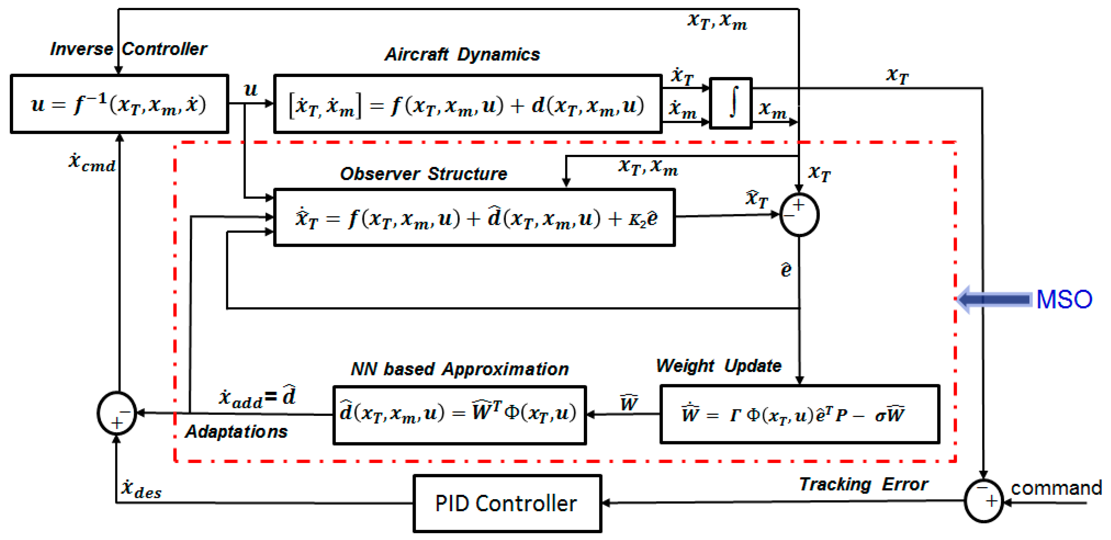
2. Modified State Observer Architecture

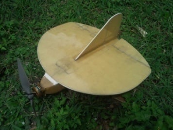
3. Aircraft Model


| Serial No. | Properties | Value | Units | |
|---|---|---|---|---|
| 1 | Mass, | 0.29 | kg | |
| 2 | Wing span, b | 0.30 | m | |
| 3 | Mean Aerodynamic Chord, c | 0.25 | m | |
| 4 | Wing Surface Area, S | 0.06118 | m2 | |
| 5 | Inertia | Ixx | 0.00301326 | kg·m2 |
| Iyy | 0.00310261 | kg·m2 | ||
| Izz | 0.0002636712 | kg·m2 | ||
| Ixz | 0.000001093 | kg·m2 | ||
| 6 | Moment Reference Position | (0.074,0,0) | m | |
3.1. Linear Accelerations
3.2. Angular Accelerations
3.3. Angular Rates
3.4. Aerodynamic Forces and Moments
3.5. Force Coefficients
3.6. Moment Coefficients
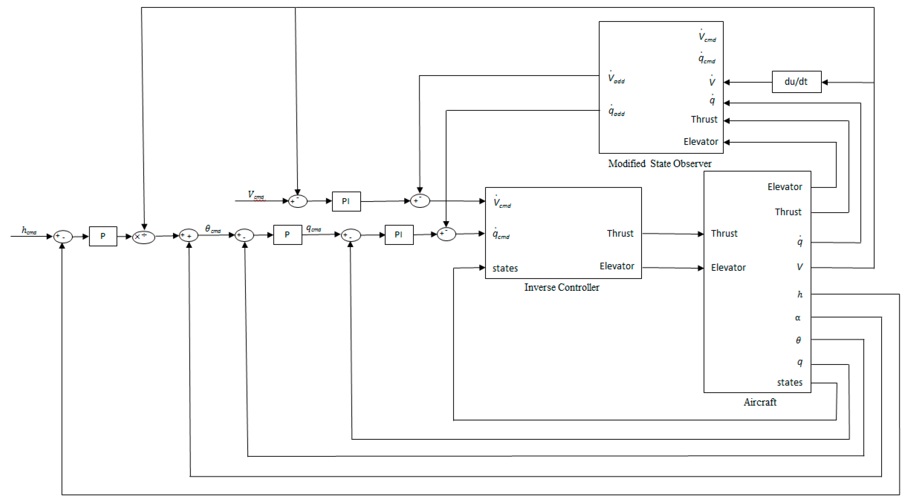
4. Dynamic Inverse Controller Design

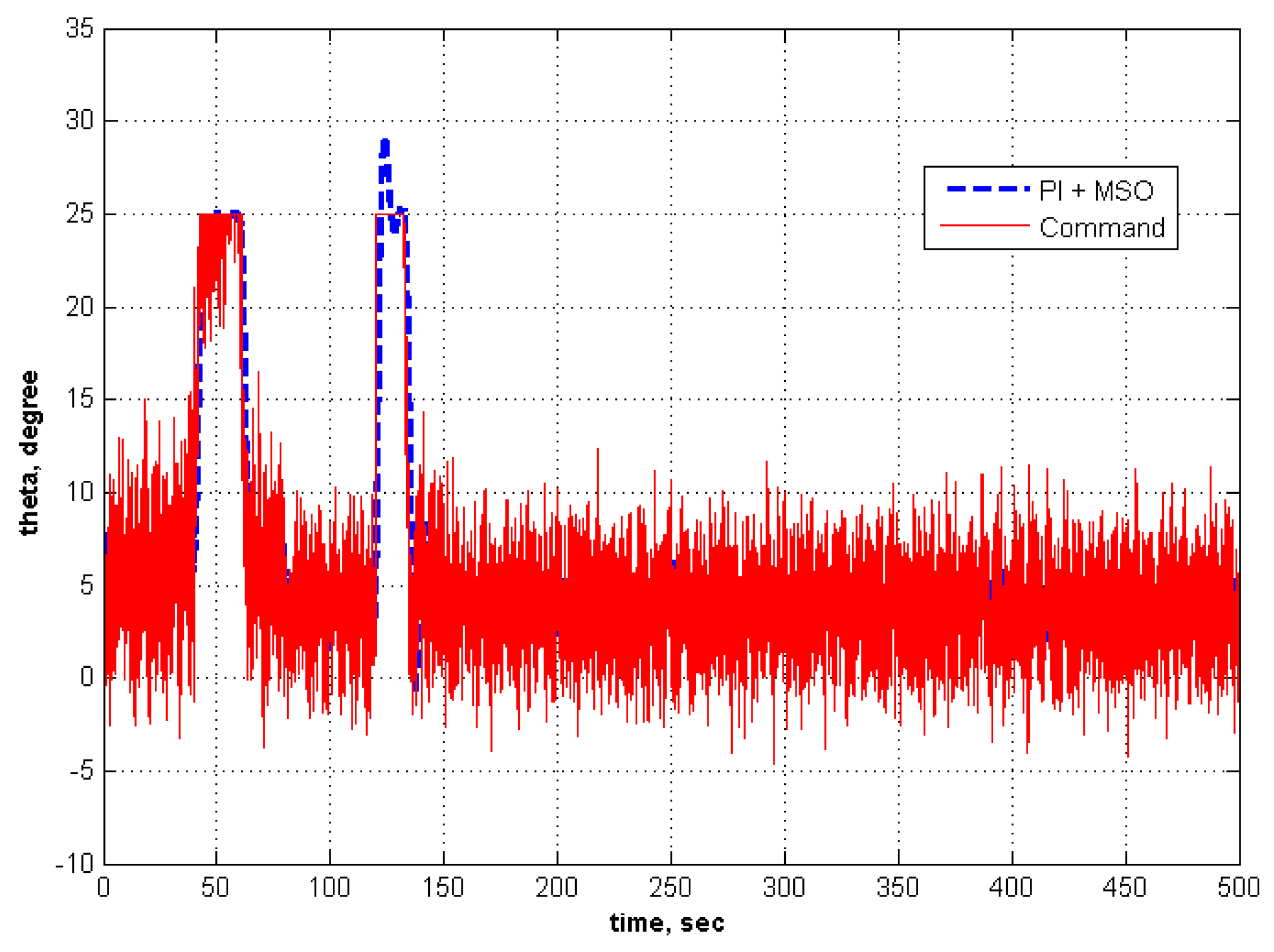
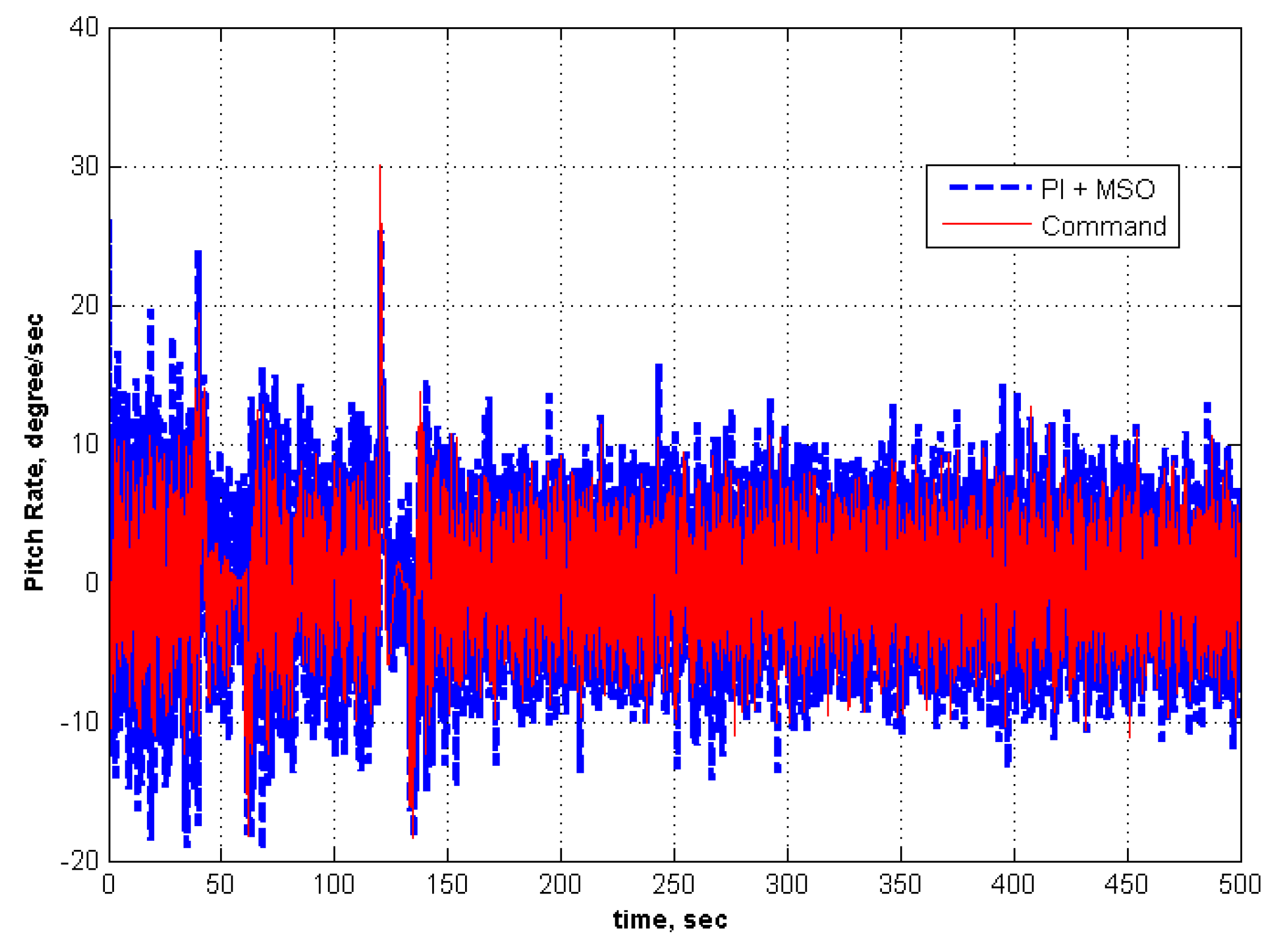
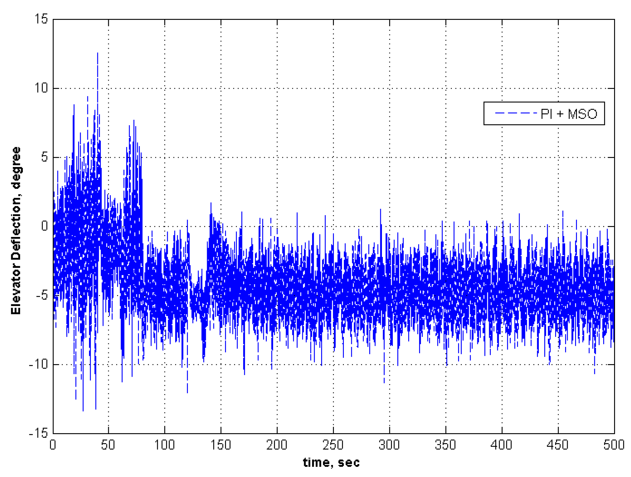
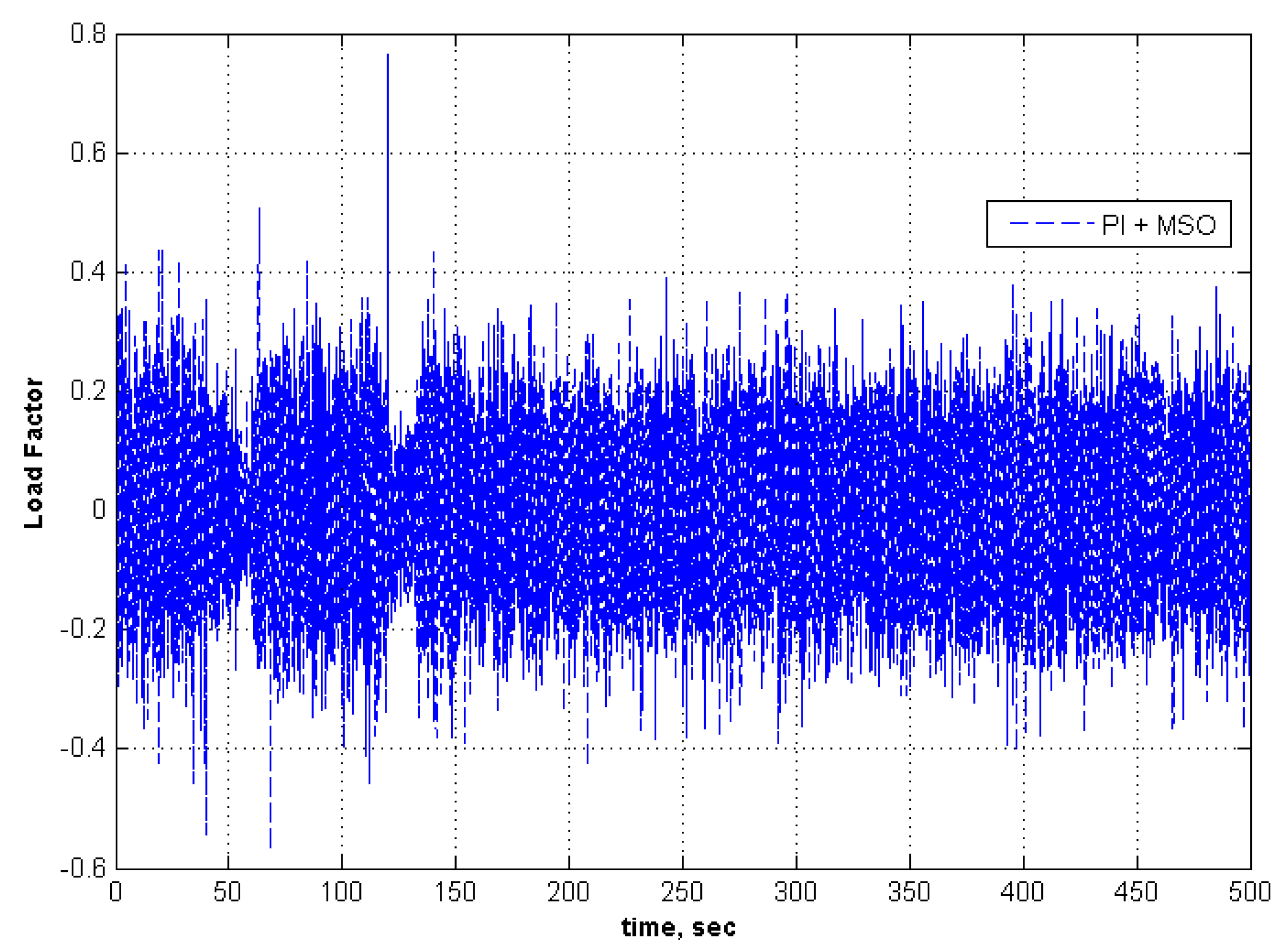
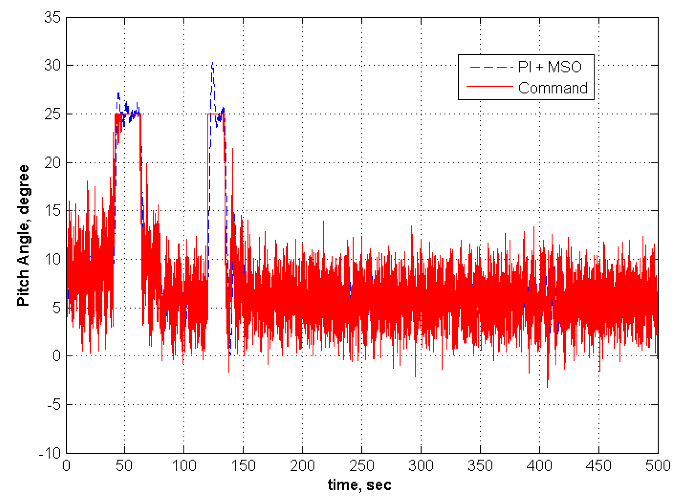
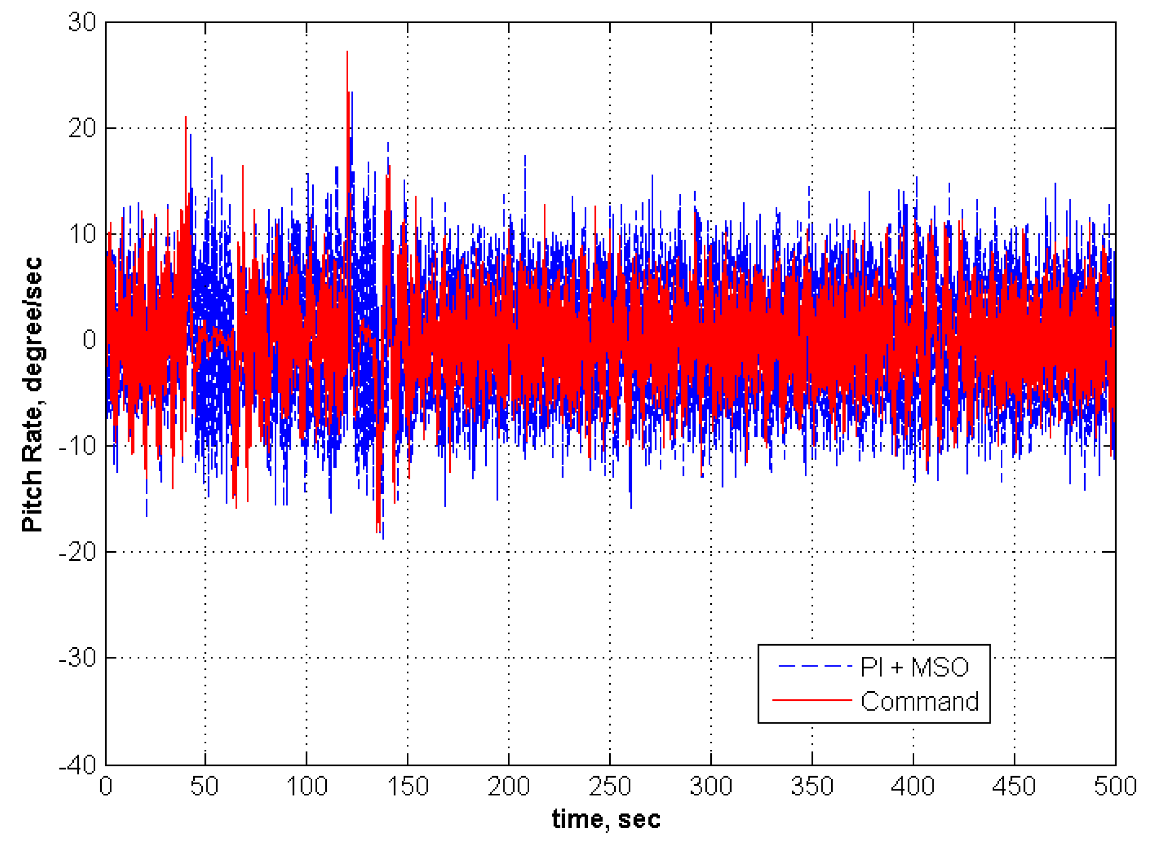
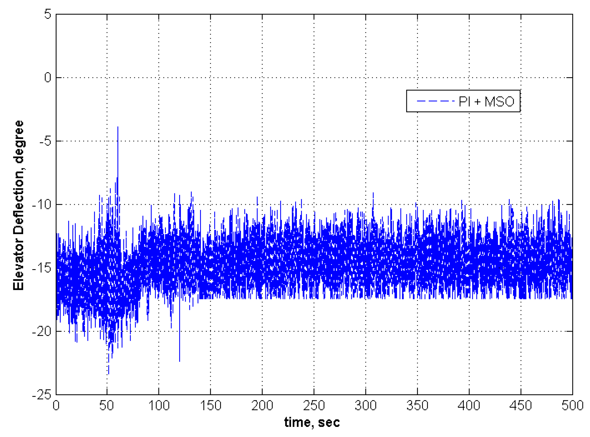
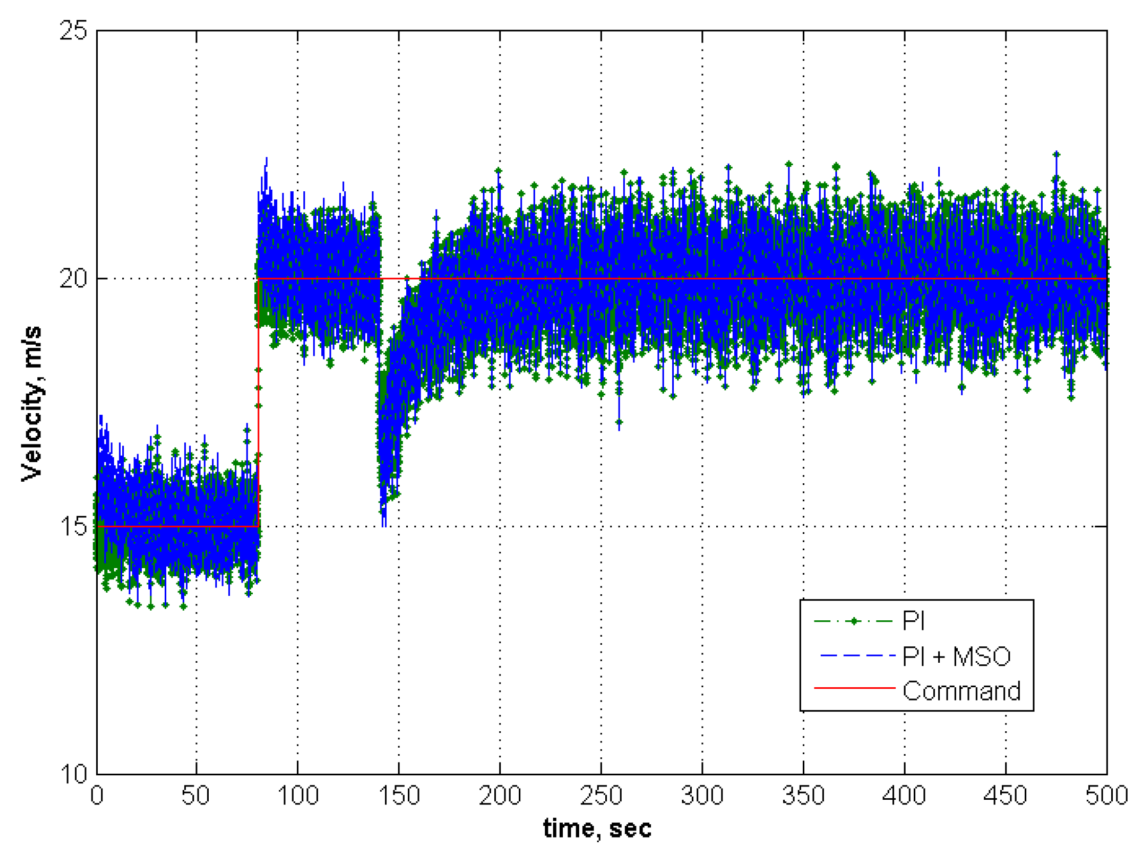
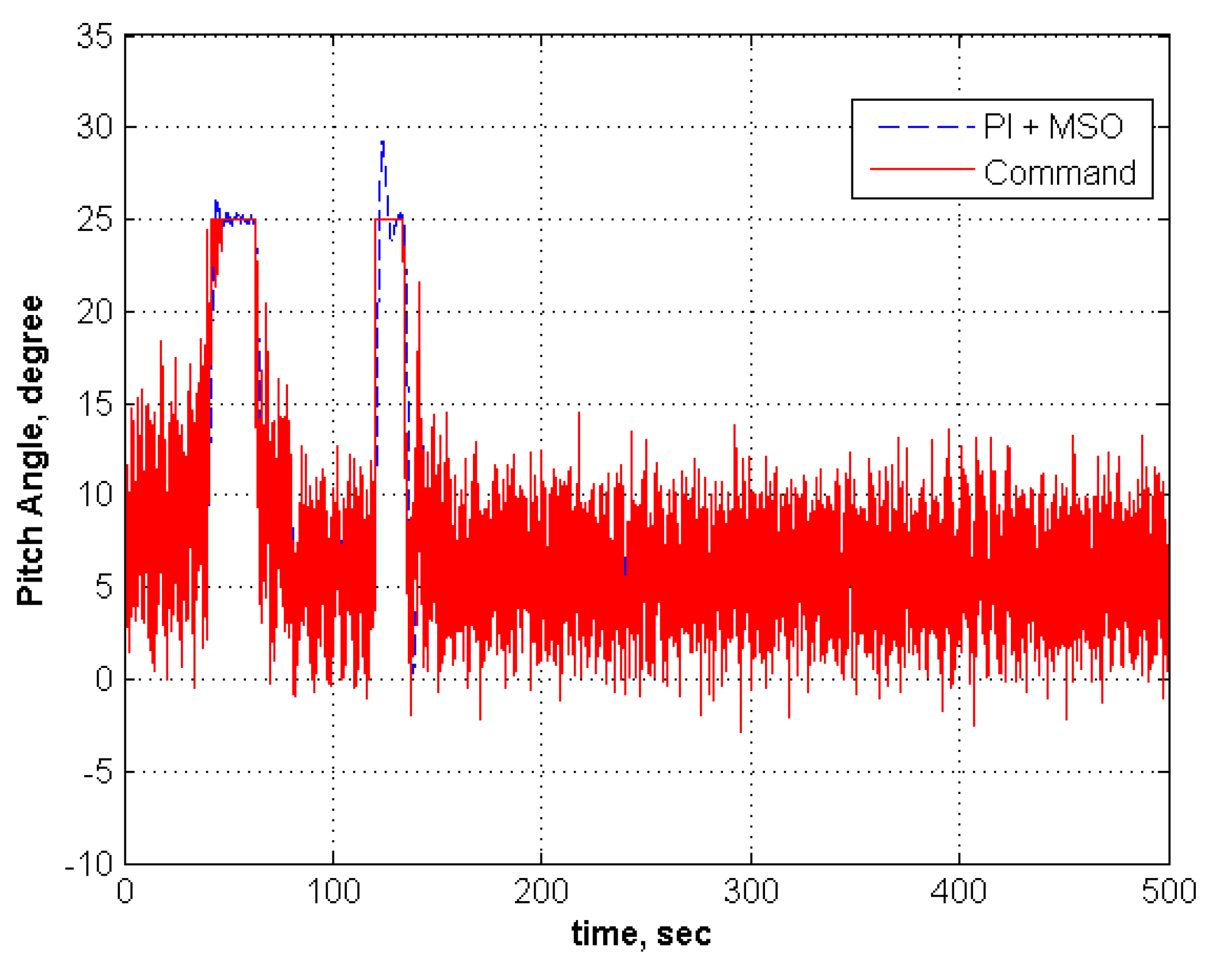
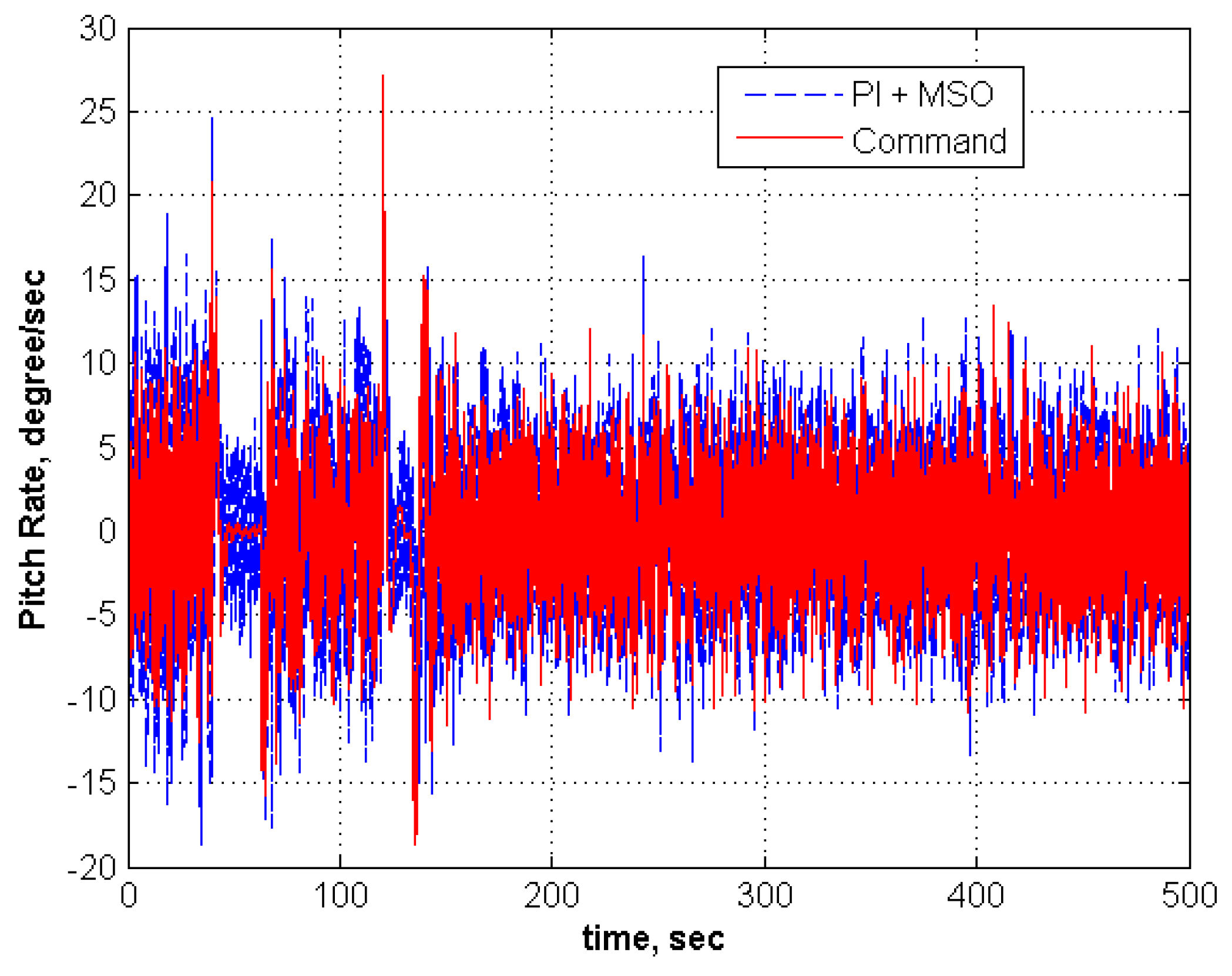
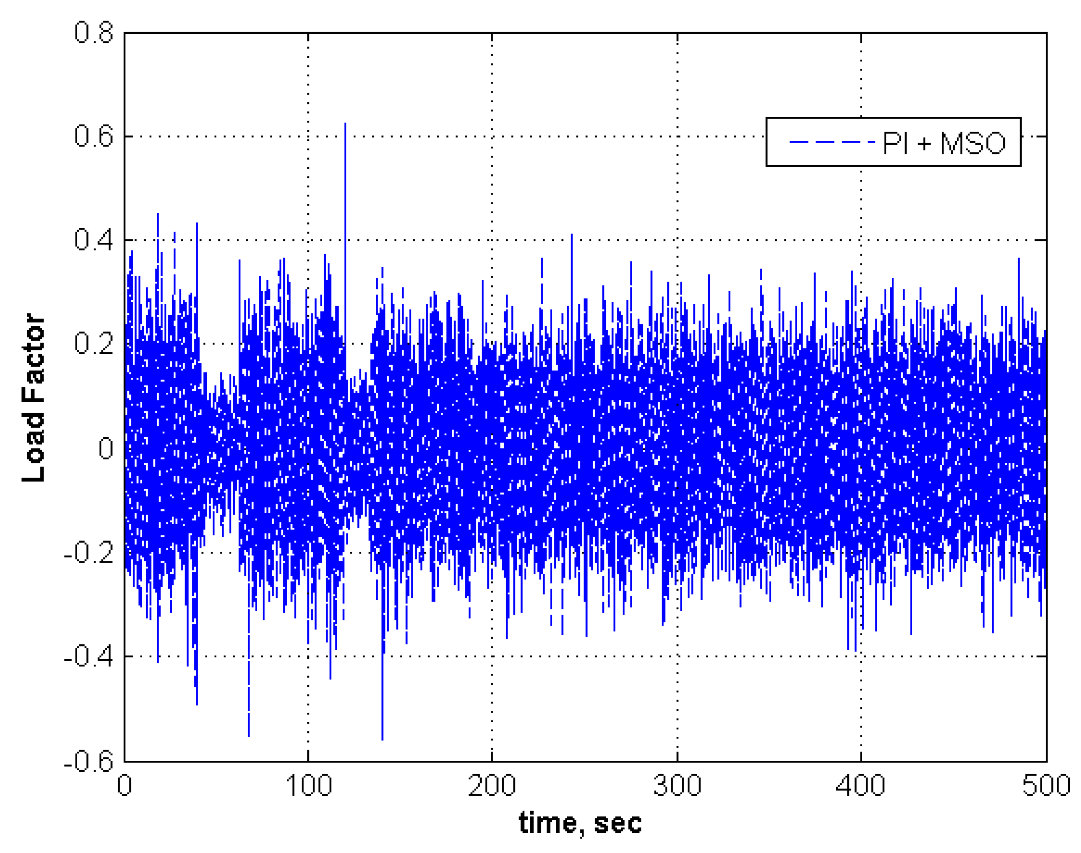
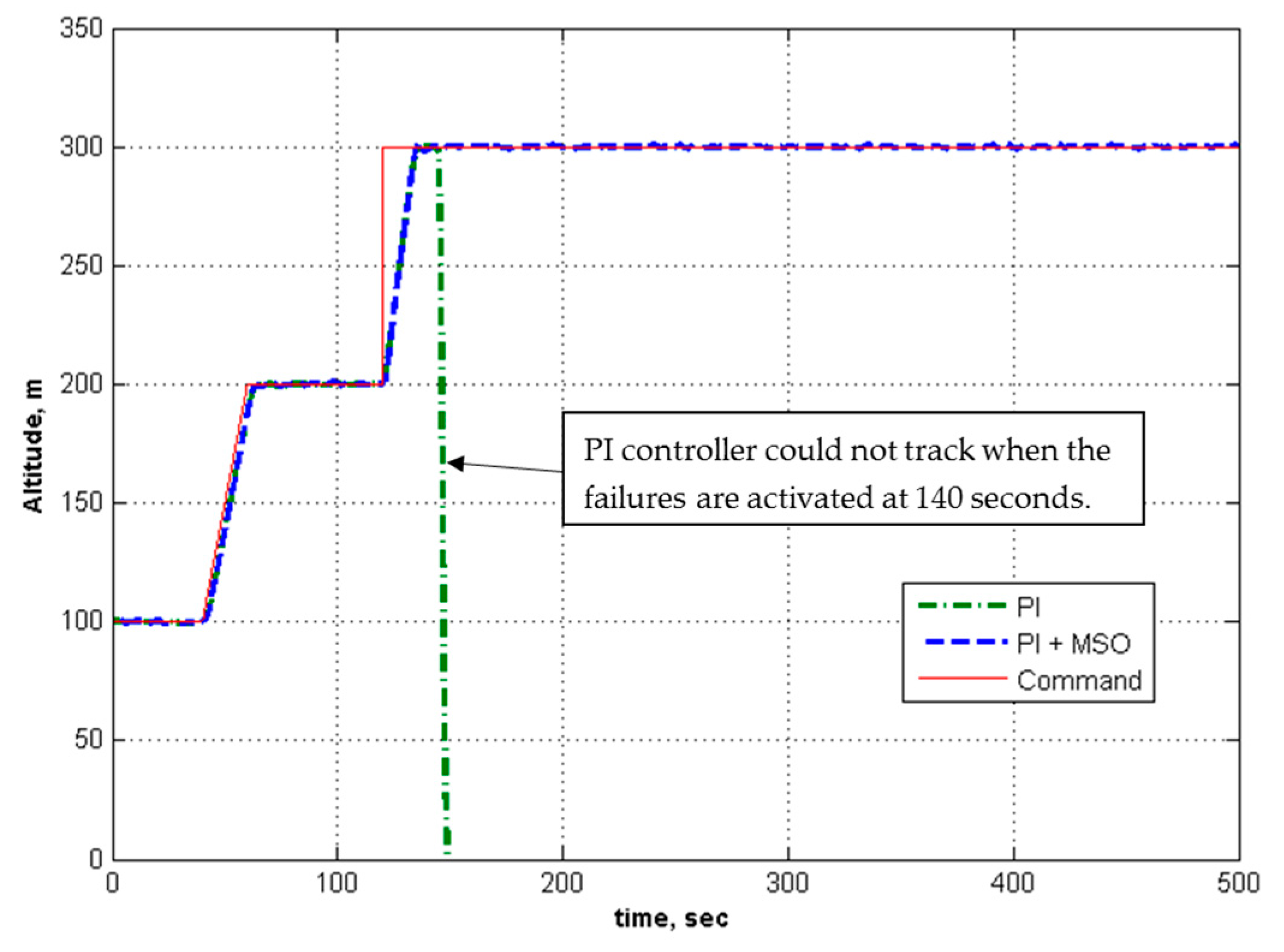
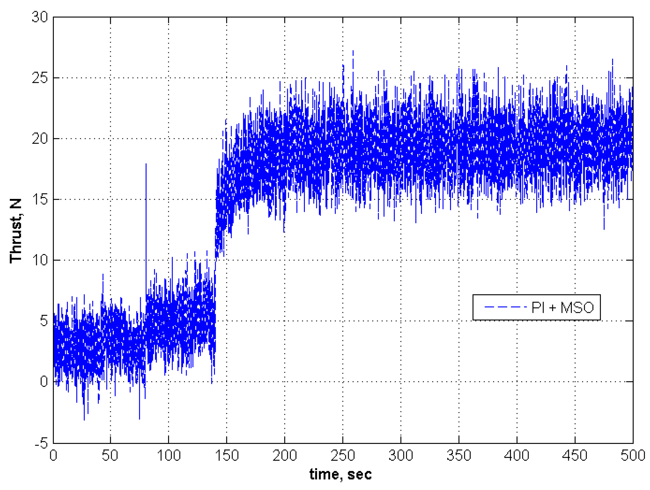
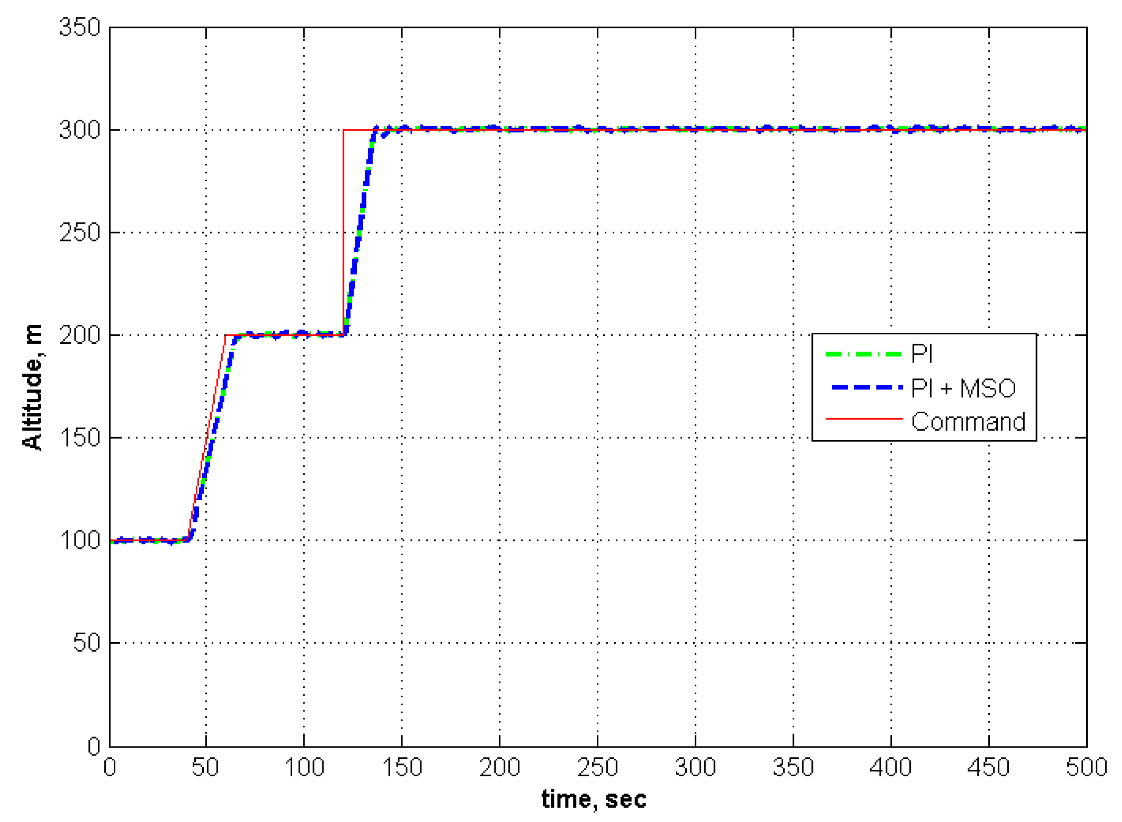
5. Simulation Results
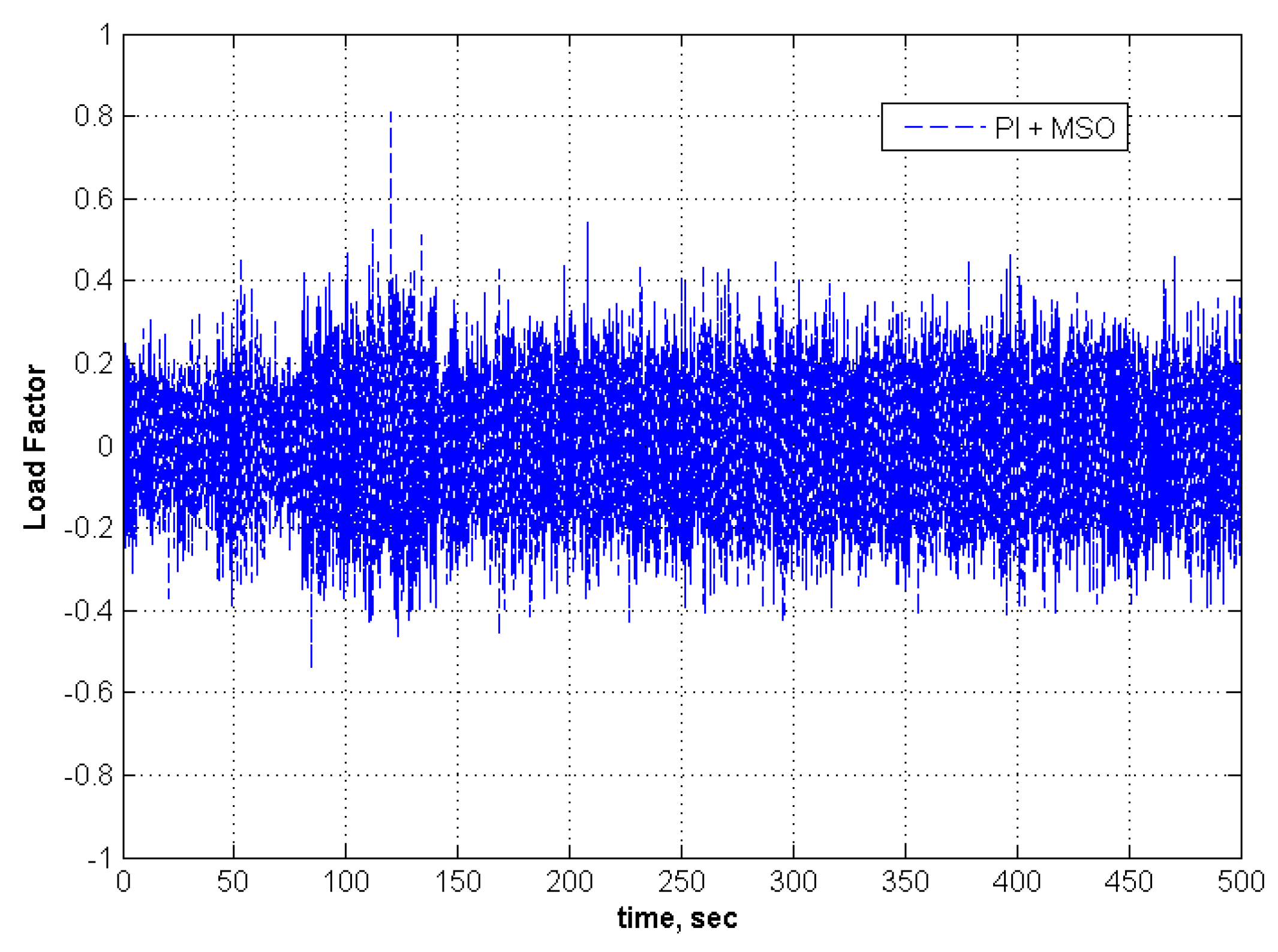
| Level | Absolute Load Factor (nZ) Centered around 1g | Explanation |
|---|---|---|
| Very Low | Below ±0.05 | Light oscillations |
| Low | ±0.05 to ±0.20 | Choppy; slight, rapid, rhythmic bumps or cobble-stoning |
| Moderate | ±0.20 to ±0.50 | Strong intermittent jolts |
| Severe | ±0.50 to ±1.50 | Aircraft handling made difficult |
| Very Severe | Above ±1.50 | Increasing handling difficulty, possible structural damage |
- No Modeling Errors
- Modeling Error in Aircraft
- Modeling Error in Inverse Controller
5.1. Adaptation for No Modeling Error
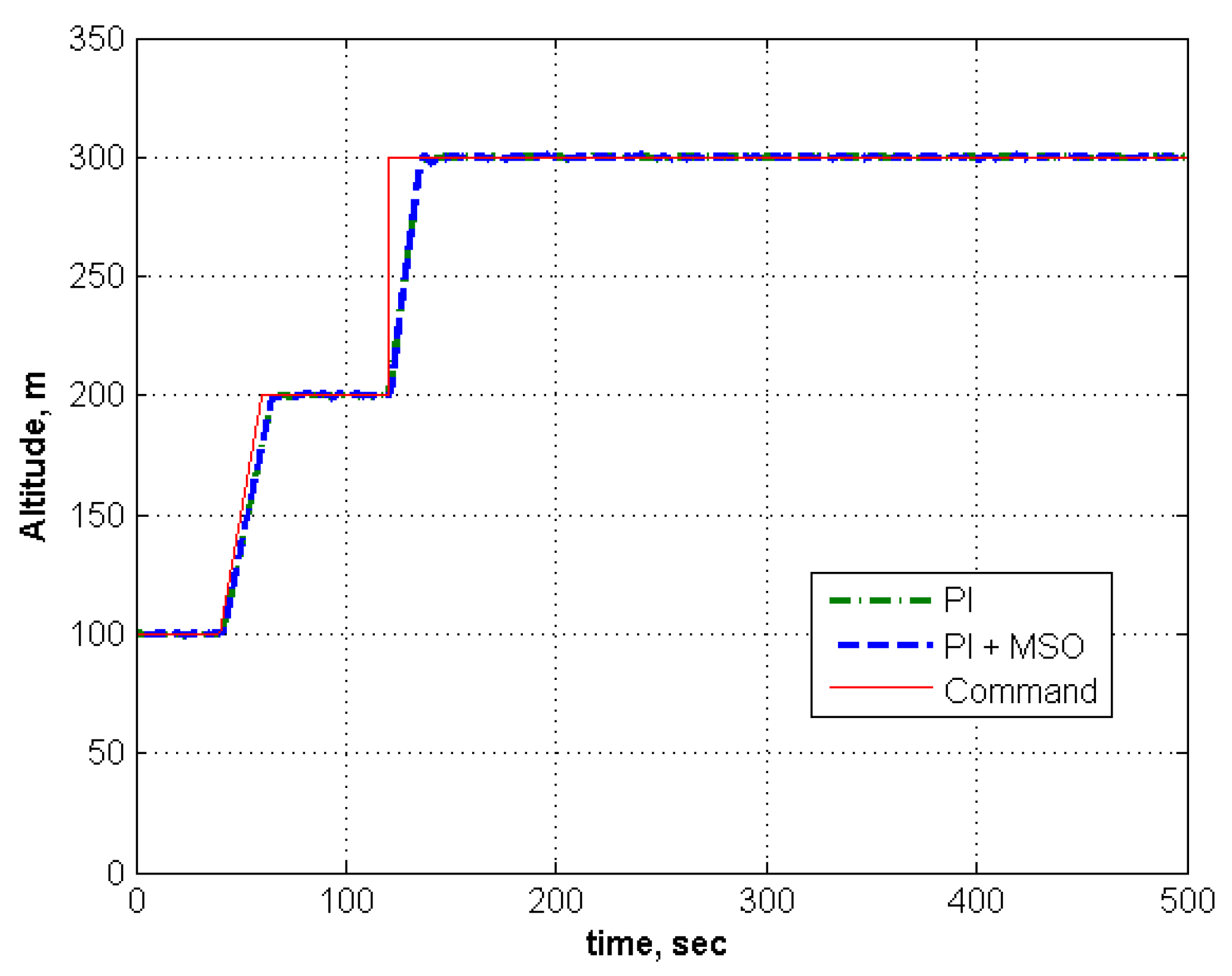
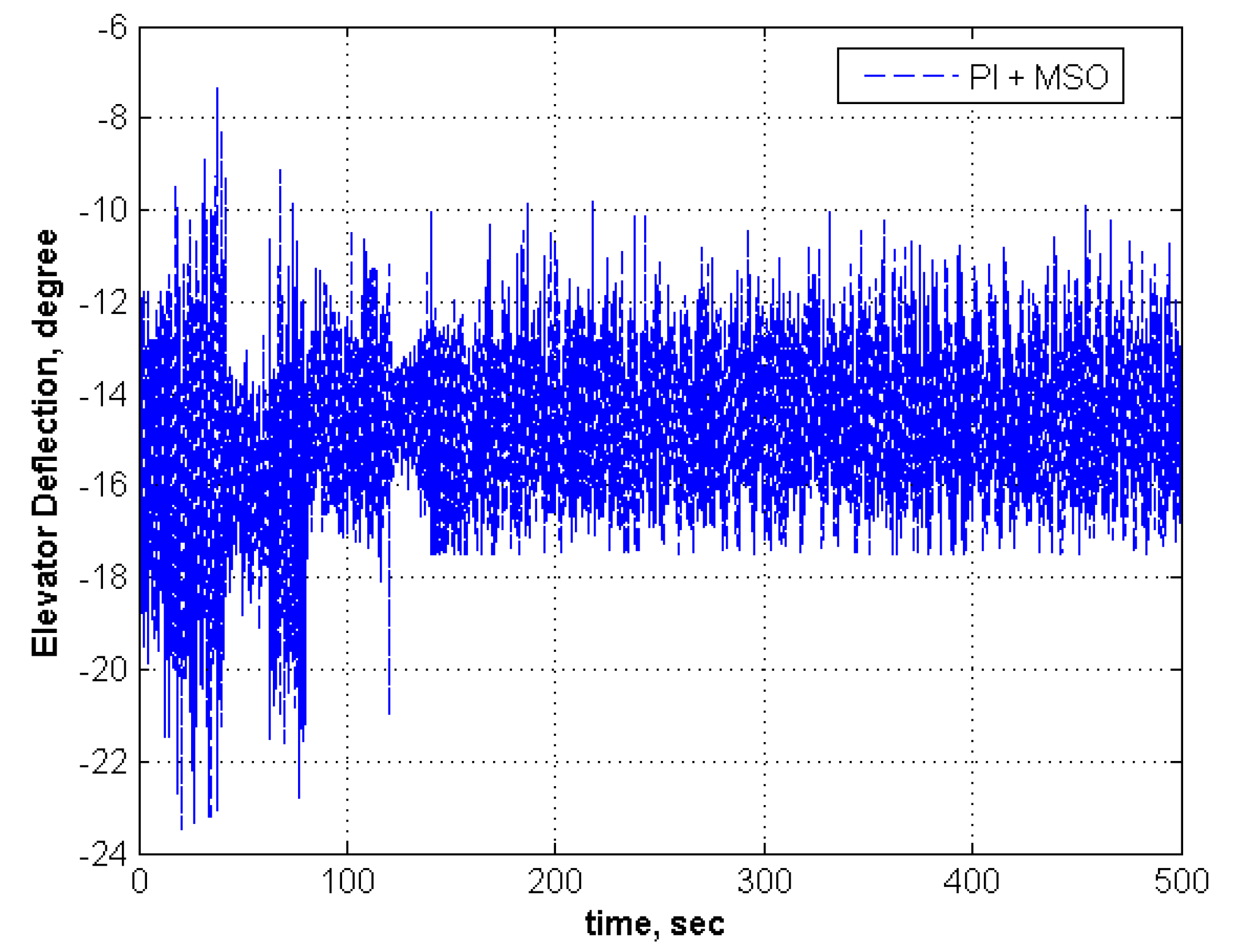
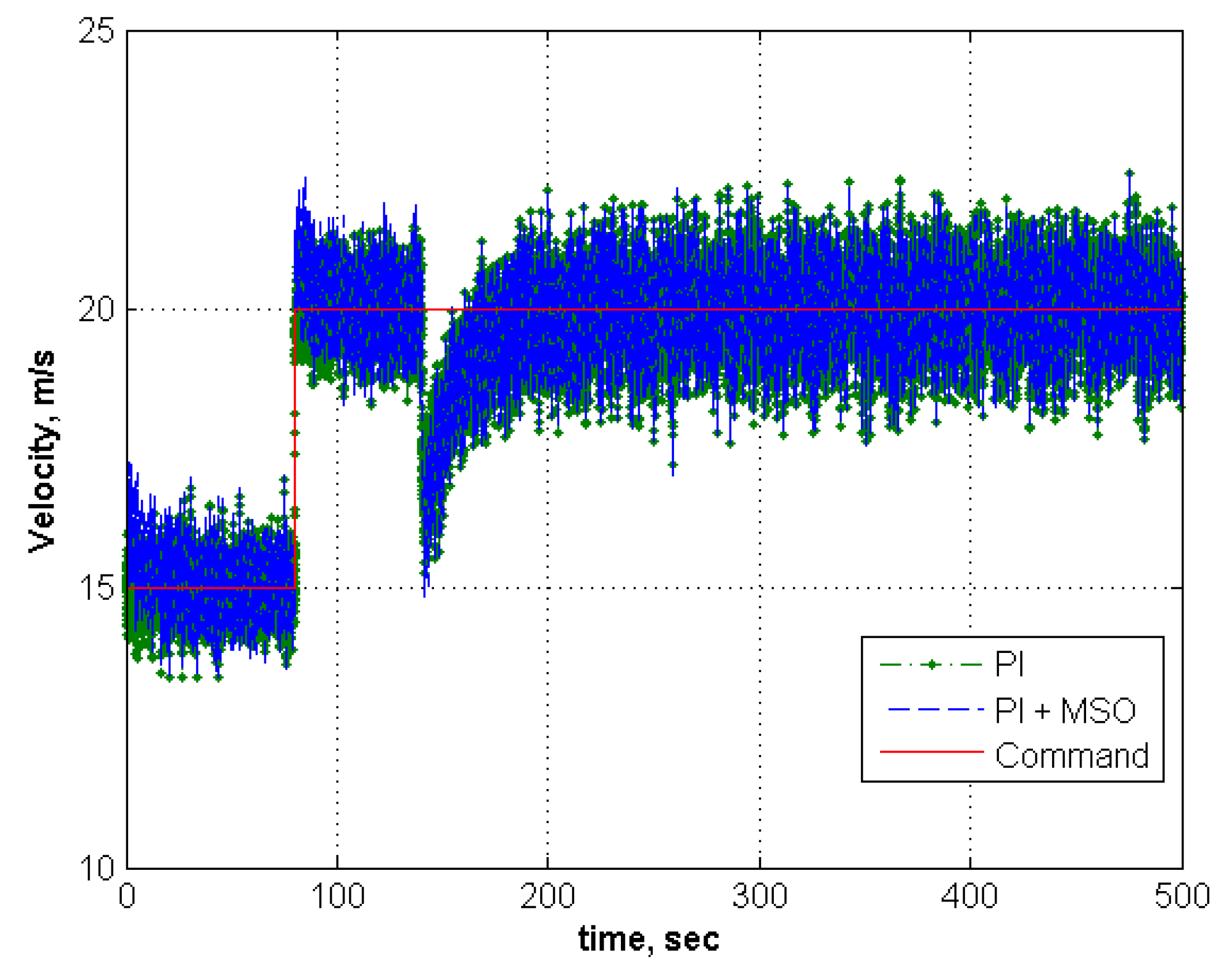
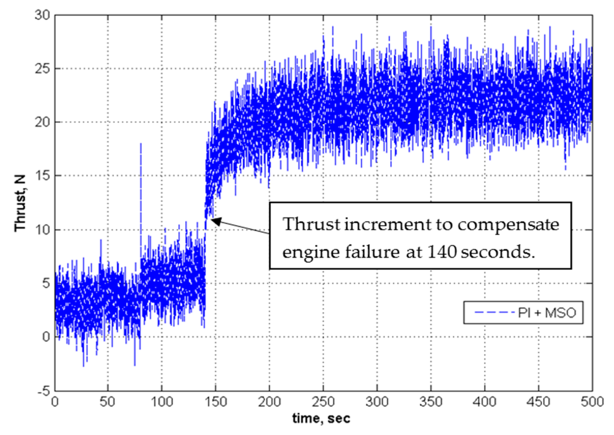
| Case | —Aircraft * | —Controller * | Elevator Failure, % | Engine Failure, % | Turbulence | Result | ||||
|---|---|---|---|---|---|---|---|---|---|---|
| L, m | σw, m/s | Without MSO | nZ | With MSO | nZ | |||||
| 1 | −1 | −1 | None | None | None | None | Tracks | NA | NA | NA |
| 2 | −1 | −1 | 30 | 75 | None | None | Tracks | NA | NA | NA |
| 3 | −1 | −1 | 40 | 75 | None | None | Fails | NA | Fails | NA |
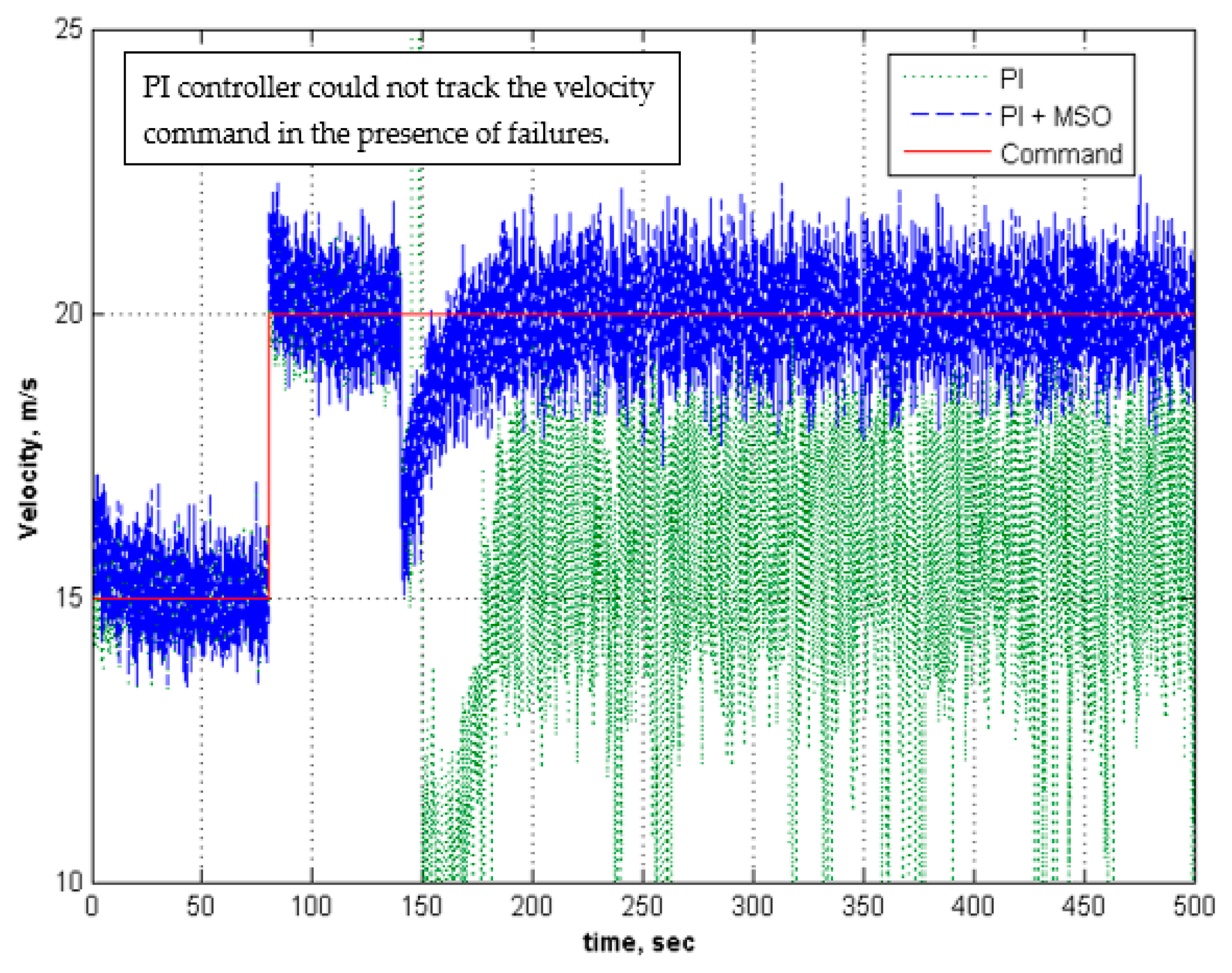
| 4 | −1 | −1 | None | None | 2 | 5 | Tracks | Moderate | Tracks | Low |
| 0.2 to 0.3 | 0.1 to 0.2 | |||||||||
| 5 | −1 | −1 | 30 | 75 | 2 | 5 | Tracks | Moderate | Tracks | Low |
| 0.2 to 0.3 | 0.1 to 0.2 | |||||||||
| 6 | −1 | −1 | 40 | 75 | 2 | 5 | Fails | NA | Fails | NA |


5.2. Adaptation for Modeling Error in an Aircraft
| Case | —Aircraft * | —Controller * | Elevator Failure, % | Engine Failure, % | Turbulence | Result | ||||
|---|---|---|---|---|---|---|---|---|---|---|
| L, m | σw, m/s | Without MSO | nZ | With MSO | nZ | |||||
| 1 | −0.5 | −1 | None | None | None | None | Tracks | NA | NA | NA |
| 2 | −0.5 | −1 | 40 | 75 | None | None | Fails | NA | Tracks | NA |
| 3 | −0.5 | −1 | None | None | 2 | 5 | Fails | NA | Tracks | Low |
| 0.1 to 0.2 | ||||||||||
| 4 | −0.5 | −1 | 30 | 75 | 2 | 5 | Fails | NA | Tracks | Low |
| 0.1 to 0.2 | ||||||||||
| 5 | −0.5 | −1 | 40 | 75 | 2 | 5 | Fails | NA | Tracks | Low |
| 0.1 to 0.2 | ||||||||||
| 6 | −1.5 | −1 | None | None | None | None | Fails | NA | Fails | NA |
| 7 | 1 | −1 | None | None | None | None | Fails | NA | Fails | NA |


5.3. Adaptation for Modeling Error in the Controller
| Case | —Aircraft * | —Controller * | Elevator Failure, % | Engine Failure, % | Turbulence | Result | ||||
|---|---|---|---|---|---|---|---|---|---|---|
| L, m | σw, m/s | Without MSO | nZ | With MSO | nZ | |||||
| 1 | −1.0 | −0.5 | None | None | None | None | Tracks | NA | NA | NA |
| 2 | −1.0 | −0.5 | 30 | 75 | None | None | Tracks | NA | NA | NA |
| 3 | −1.0 | −0.5 | 40 | 75 | None | None | Fails | NA | Fails | NA |
| 4 | −1.0 | −0.5 | None | None | 2 | 5 | Tracks | Moderate | Tracks | Low |
| ±0.2 to ±0.5 | ±0.1 to ±0.2 | |||||||||
| 5 | −1.0 | −0.5 | 30 | 75 | 2 | 5 | Tracks | Moderate | Tracks | Low |
| ±0.2 to ±0.5 | ±0.1 to ±0.2 | |||||||||
| 6 | −1.0 | −0.5 | 40 | 75 | 2 | 5 | Fails | NA | Fails | NA |
| 7 | −1.0 | −1.5 | None | None | None | None | Fails | NA | Tracks | NA |
| 8 | −1.0 | −1.5 | 30 | 75 | None | None | Fails | NA | Tracks | NA |
| 9 | −1.0 | −1.5 | 40 | 75 | None | None | Fails | NA | Fails | NA |
| 10 | −1.0 | −1.5 | None | None | 2 | 5 | Fails | NA | Fails | NA |


6. Conclusions
Acknowledgments
Author Contributions
Conflicts of Interest
Appendix
Derivation of Accelerations and Angular Rates:
References
- Pesonen, U.J.; Steck, J.E.; Rokhsaz, K.; Bruner, H.S.; Duerksen, N. Adaptive Neural Network Inverse Controller for General Aviation Safety. J. Guid. Control Dyn. 2004, 27, 434–443. [Google Scholar] [CrossRef]
- Lemon, K.A.; Steck, J.E.; Hinson, B.T.; Rokhsaz, K.; Nguyen, N.; Kimball, D. Model Reference Adaptive Fight Control Adapted for General Aviation: Controller Gain Simulation and Preliminary Flight Testing on a Bonanza Fly-by-Wire Testbed. In Proceedings of the AIAA Guidance, Navigation, and Control Conference, Toronto, ON, Canada, 2–5 August 2010.
- Lemon, K.A.; Steck, J.E.; Hinson, B.T.; Rokhsaz, K.; Nguyen, N. Application of a Six Degree of Freedom Adaptive Controller to a General Aviation Aircraft. In Proceedings of the AIAA Guidance, Navigation, and Control Conference, Portland, OR, USA, 8–11 August 2011.
- Arning, R.K.; Sassen, S. Flight Control of Micro Aerial Vehicles. In Proceedings of the AIAA Guidance, Navigation, and Control Conference and Exhibit, Providence, RI, USA, 16–19 August 2004.
- Jordan, T.L.; Foster, J.V.; Bailey, R.M.; Belcastro, C.M. AirSTAR: A UAV Platform for Flight Dynamics and Control System Testing. In Proceedings of the 25th AIAA Aerodynamic Measurement Technology and Ground Testing Conference, San Francisco, CA, USA, 5–8 June 2006.
- Knoebel, N.B.; Osborne, S.R.; Matthews, J.S.; Eldredge, A.M.; Beard, R.W. Computationally Simple Model Reference Adaptive Control for Miniature Air Vehicles. In Proceedings of the 2006 American Control Conference, Minneapolis, MN, USA, 14–16 June 2006.
- Beard, R.W.; Knoebel, N.; Cao, C.; Hovakimyan, N.; Matthews, J. An L1 Adaptive Pitch Controller for Miniature Air Vehicles. In Proceedings of the AIAA Guidance, Navigation, and Control Conference and Exhibit, Keystone, CO, USA, 21–24 August 2006.
- Ismail, S.; Pashilkar, A.A.; Ayyagari, R. Adaptive Control of Micro Aerial Vehicles. In Proceedings of the Symposium on Applied Aerodynamics and Design of Aerospace Vehicle (SAROD 2011), Bangalore, India, 16–18 November 2011.
- Waszak, M.R.; Davidson, J.B.; Ifju, P.G. Simulation and Flight Control of an Aeroelastic Fixed Wing Micro Aerial Vehicle. In Proceedings of the AIAA Atmospheric Flight Mechanics Conference and Exhibit, Monterey, CA, USA, 5–8 August 2002.
- Bacon, B.J.; Ostroff, A.J. Reconfigurable Flight Control Using Nonlinear Dynamic Inversion with a Special Accelerometer Implementation. In Proceedings of the AIAA Guidance, Navigation and Control Conference and Exhibit, Denver, CO, USA, 14–17 August 2000.
- Kim, B.S.; Calise, A.J.; Kam, M. Nonlinear Flight Control Using Neural Networks and Feedback Linearization. In Proceedings of the Aerospce Control Systems, Westlake Village, CA, USA, 25–27 May 1993.
- McFarland, M.B.; Calise, A.J. Robust Adaptive Control of Uncertain Nonlinear Systems Using Neural Networks. In Proceedings of the American Control Conference, Albuquerque, NM, USA, 4–6 June 1997.
- Calise, A.J. Neural Networks in Nonlinear Aircraft Flight Control. In Proceedings of the WESCON-95, San Francisco, CA, USA, 7–9 November 1995.
- Gundy-Burlet, K.; Krishnakumar, K.; Limes, G.; Bryant, D. Control Reallocation Strategies for Damage Adaptation in Transport Class Aircraft. In Proceedings of the AIAA Guidance, Navigation, and Control Conference and Exhibit, Austin, TX, USA, 11–14 August 2003.
- Johnson, E.N.; Calise, A.J.; Corban, J.E. Reusable Launch Vehicle Adaptive Guidance and Control Using Neural Networks. In Proceedings of the AIAA Guidance, Navigation and Control Conference and Exhibit, Montreal, QC, Canada, 6–9 August 2001.
- Johnson, E.N.; Kannan, S.K. Adaptive Trajectory Control for Autonomous Helicopters. J. Guid. Control Dyn. 2005, 28, 524–538. [Google Scholar] [CrossRef]
- Cao, C.; Hovakimyan, N. Design and Analysis of a Novel L1 Adaptive Controller, Part I: Control Signal and Asymptotic Stability. In Proceedings of the American Control Conference, Minneapolis, MN, USA, 14–16 June 2006.
- Cao, C.; Hovakimyan, N. Design and Analysis of a Novel L1 Adaptive Controller, Part II: Guaranteed Transient Performance. In Proceedings of the American Control Conference, Minneapolis, MN, USA, 14–16 June 2006.
- Gregory, I.M.; Cao, C.; Xargay, E.; Zou, X. L1 Adaptive Control Design for NASA AirSTAR Flight Test Vehicle. In Proceedings of the AIAA Guidance, Navigation and Control Conference, Chicago, IL, USA, 10–13 August 2009.
- Gregory, I.M.; Xargay, E.; Cao, C.; Hovakimyan, N. Flight Test of an L1 Adaptive Controller on the NASA AirSTAR Flight Test Vehicle. In Proceedings of the AIAA Guidance, Navigation and Control Conference, Toronto, ON, Canada, 2–5 August 2010.
- Kaminer, I.; Pascoal, A.; Xargay, E.; Hovakimyan, N.; Cao, C.; Dobrokhodov, V. Path Following for Unmanned Aerial Vehicles Using L1 Adaptive Augmentation of Commercial Autopilots. J. Guid. Control Dyn. 2010, 33, 550–564. [Google Scholar] [CrossRef] [Green Version]
- Wang, X.; Hovakimyan, N. L1 Adaptive Controller for Nonlinear Reference Systems. In Proceedings of the American Control Conference, San Francisco, CA, USA, 29 June–1 July 2011.
- Steck, J.E.; Rokhsaz, K.; Pesonen, U.J.; Singh, B.; Chandramohan, R. Effect of Turbulence on an Adaptive Dynamic Inverse Flight Controller. In Proceedings of the Infotech@Aerospace, Arlington, VA, USA, 26–29 September 2005.
- Rajagopal, K.; Mannava, A.; Balakrishnan, S.; Nguyen, N.; Krishnakumar, K. Neuroadaptive Model Following Controller Design for Non-affine Non-square Aircraft System. In Proceedings of the AIAA Guidance, Navigation, and Control Conference, Chicago, IL, USA, 10–13 August 2009.
- Pappu, V.S.; Steck, J.E.; Rajagopal, K.; Balakrishnan, S. Modified State Observer Based Adaptation of a General Aviation aircraft—Simulation and Flight Test. In Proceedings of the AIAA Giudance, Navigation and Control Conference, National Harbor, MD, USA, 13–17 January 2014.
- Pappu, V.S.; Steck, J.E.; Steele, B.S.; Rajagopal, K.; Balakrishnan, S. Hardware-in-Loop and Flight Testing of Modified State Observer Based Adaptation for a General Aviation Aircraft. In Proceedings of the AIAA Guidance, Navigation and Control Conference, Kissimmee, FL, USA, 5–9 January 2015.
- Roskam, J. Airplane Flight Dynamics and Automatic Flight Controls Part I. DARcorporation: Lawrence, KS, USA, 2003. [Google Scholar]
© 2016 by the authors; licensee MDPI, Basel, Switzerland. This article is an open access article distributed under the terms and conditions of the Creative Commons by Attribution (CC-BY) license (http://creativecommons.org/licenses/by/4.0/).
Share and Cite
S. R. Pappu, V.; Steck, J.E.; Ramamurthi, G. Turbulence Effects on Modified State Observer-Based Adaptive Control: Black Kite Micro Aerial Vehicle. Aerospace 2016, 3, 6. https://doi.org/10.3390/aerospace3010006
S. R. Pappu V, Steck JE, Ramamurthi G. Turbulence Effects on Modified State Observer-Based Adaptive Control: Black Kite Micro Aerial Vehicle. Aerospace. 2016; 3(1):6. https://doi.org/10.3390/aerospace3010006
Chicago/Turabian StyleS. R. Pappu, Venkatasubramani, James E. Steck, and Guruganesh Ramamurthi. 2016. "Turbulence Effects on Modified State Observer-Based Adaptive Control: Black Kite Micro Aerial Vehicle" Aerospace 3, no. 1: 6. https://doi.org/10.3390/aerospace3010006