
Target Tracking in 3-D Using Estimation Based Nonlinear Control Laws for UAVs †


Abstract
:
1. Introduction
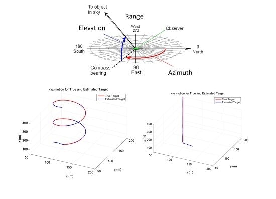
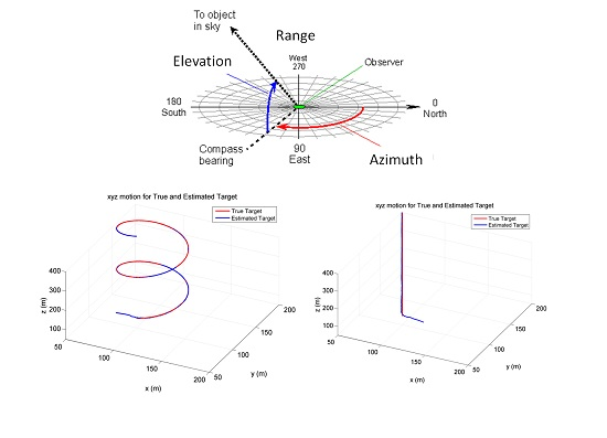
2. Problem Description
2.1. Backstepping Based Controller
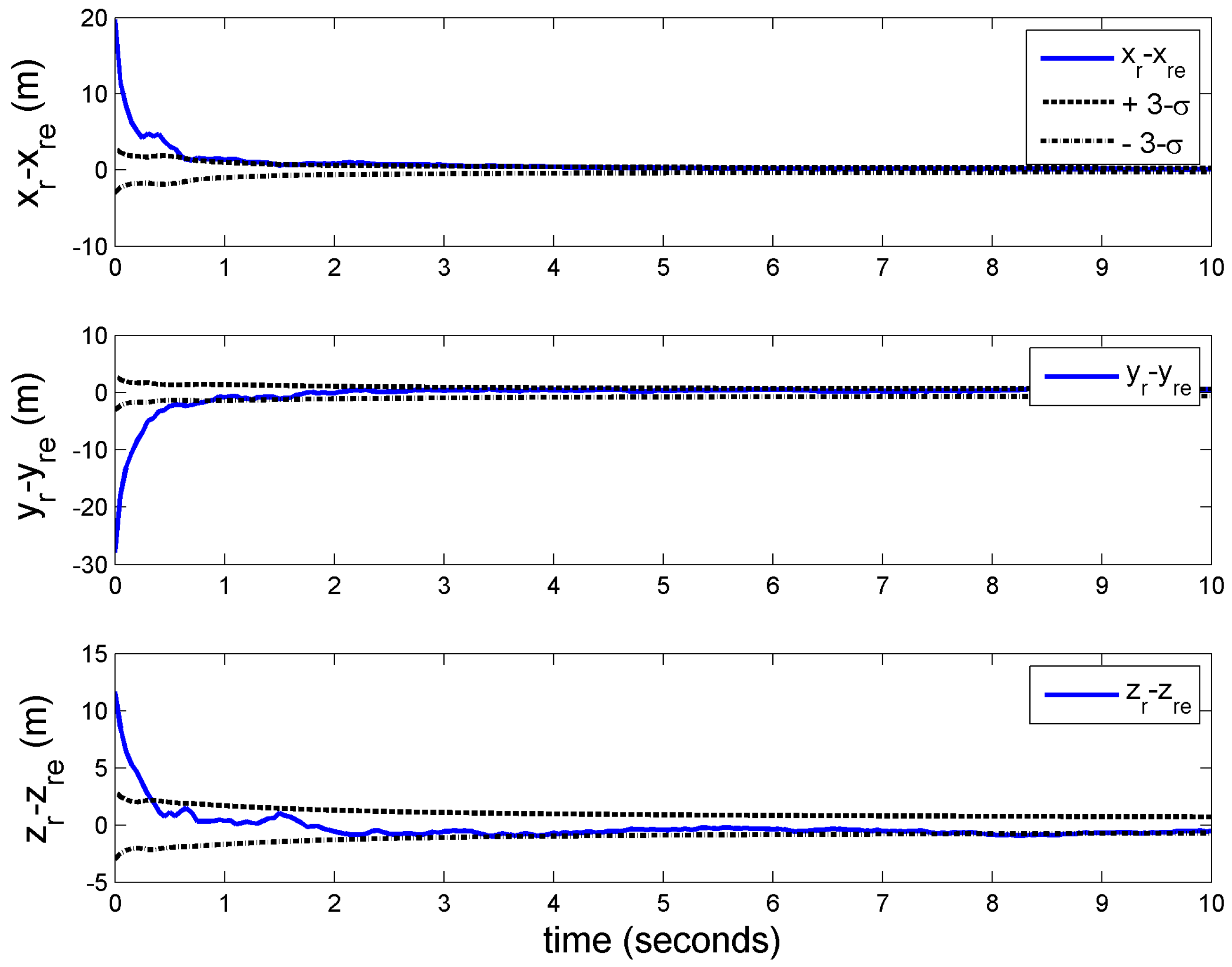
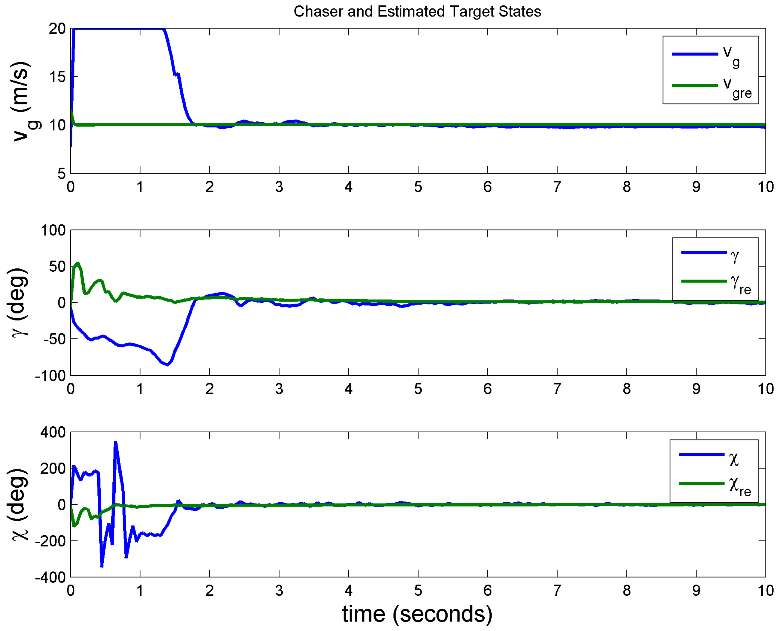
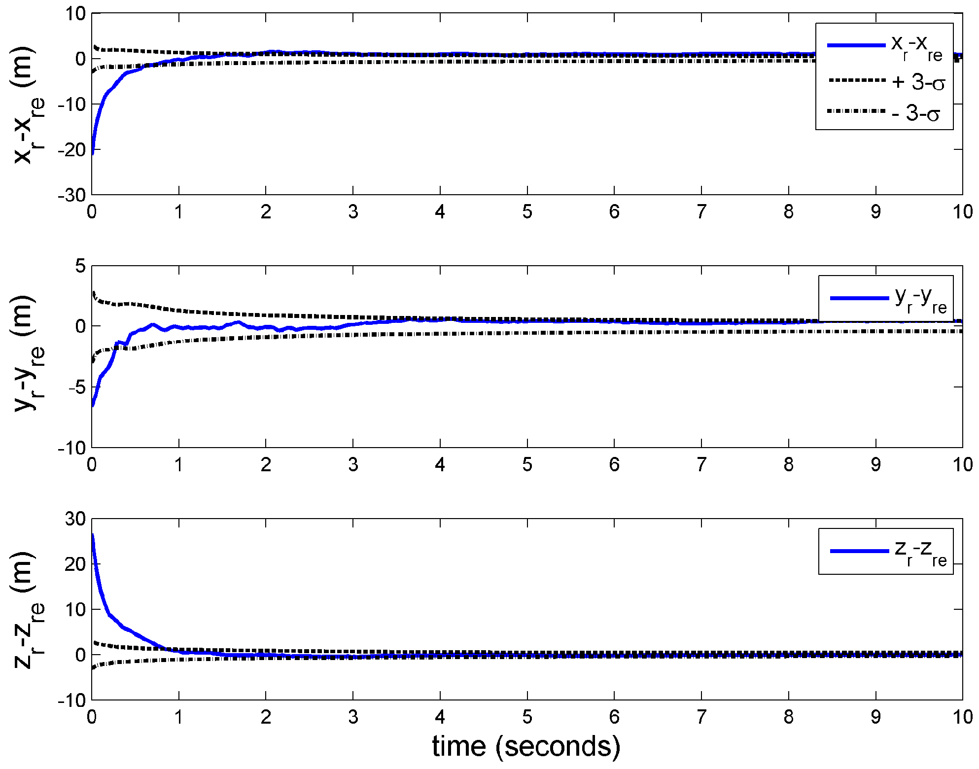
2.2. Estimation Based Controller (Partial Target Information)
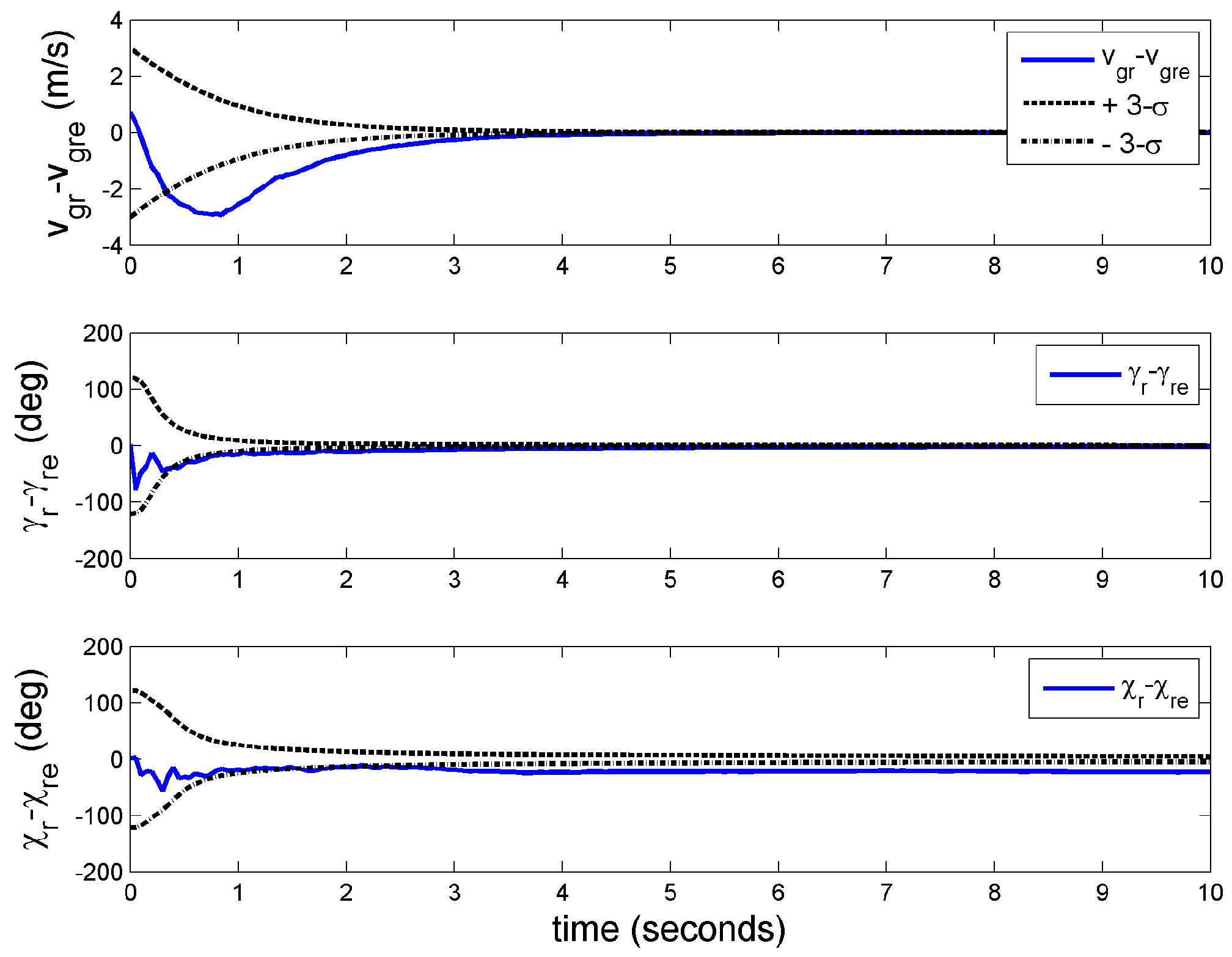
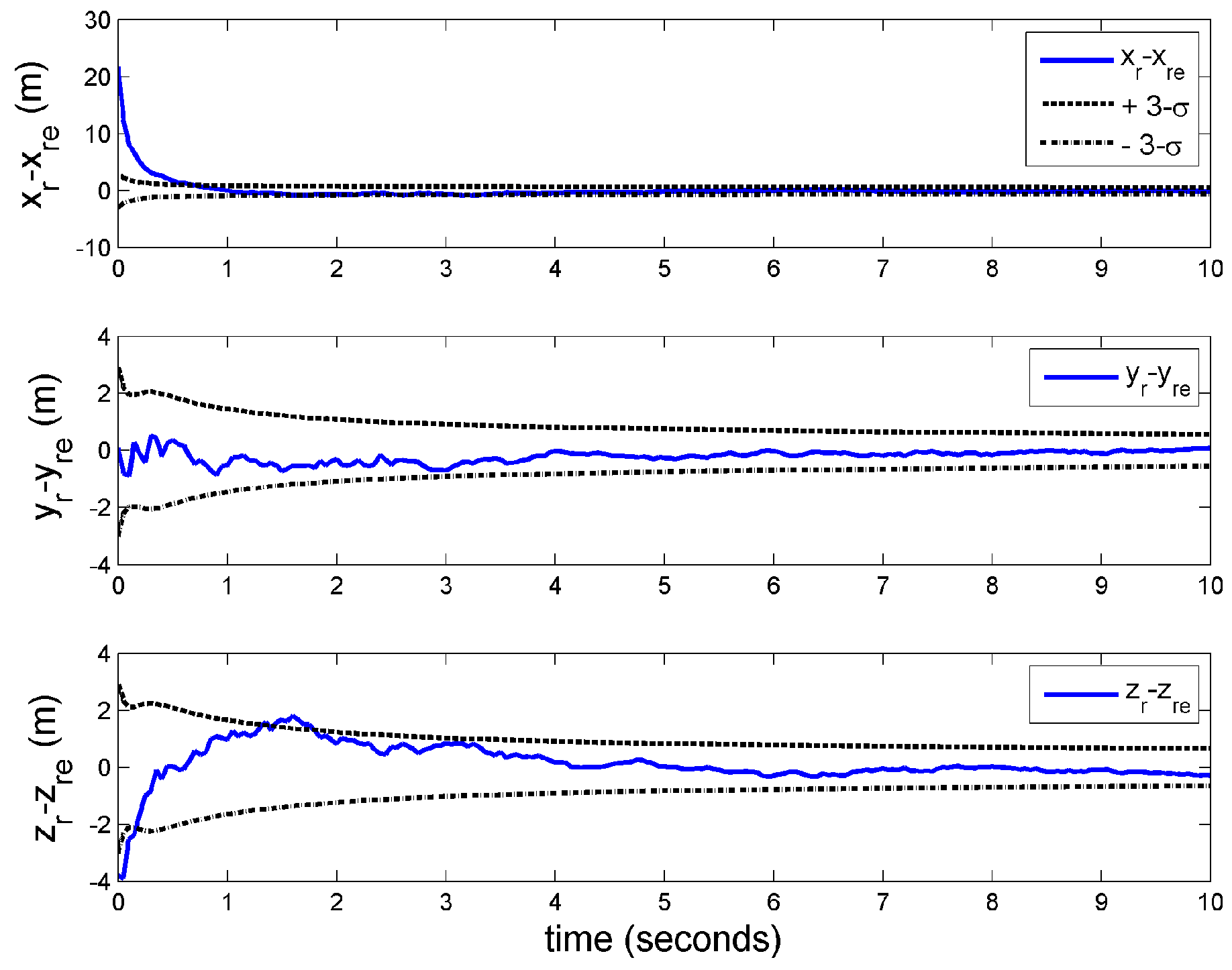
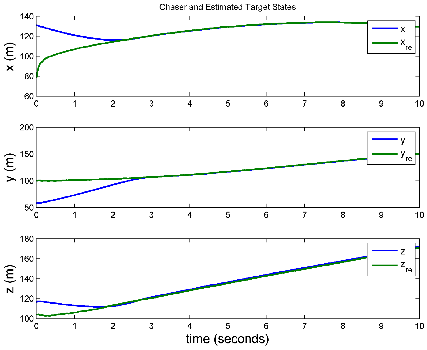
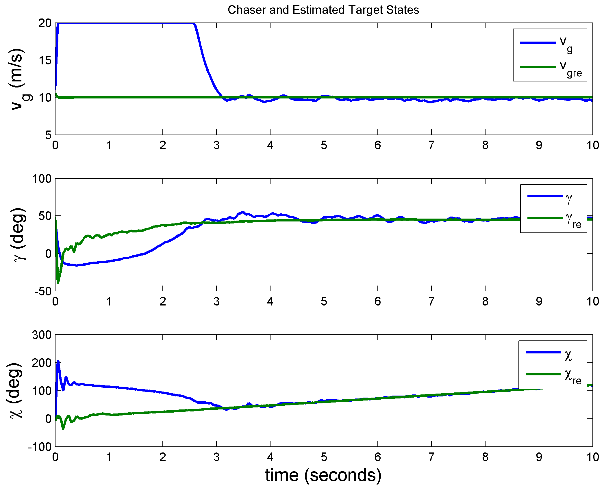
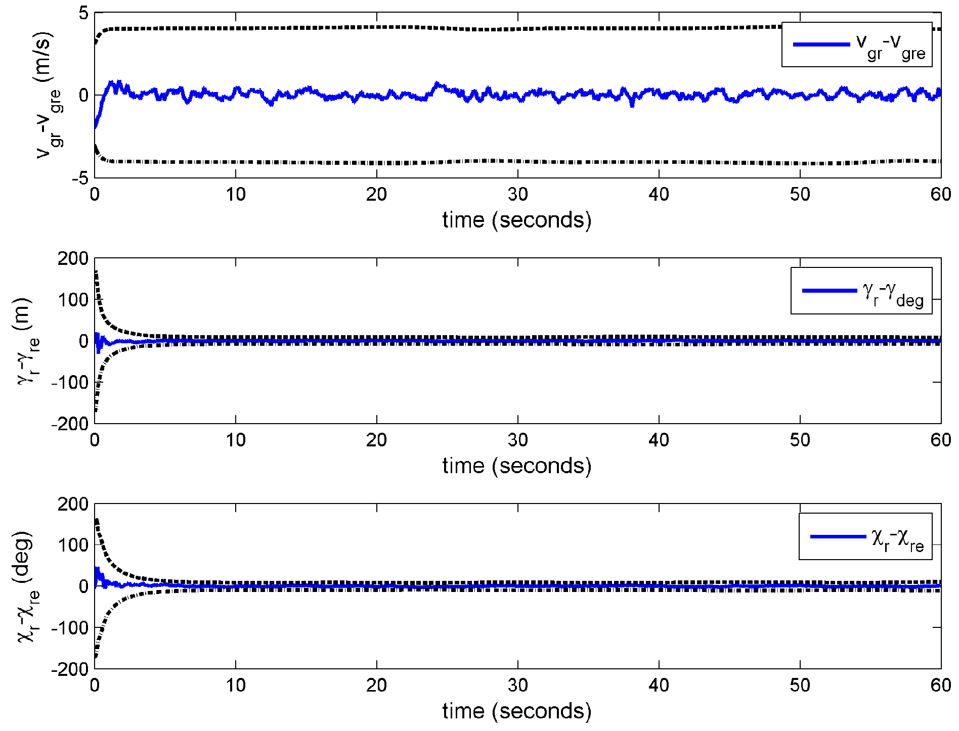
Case 1: Target measurements corrupted by stationary white noise

| Kalman gain: | |
| State update: | |
| Covariance update: | |
| Estimated state propagation is governed by: | |
| Error covariance is propagated by: | |
| Output estimate equation: |
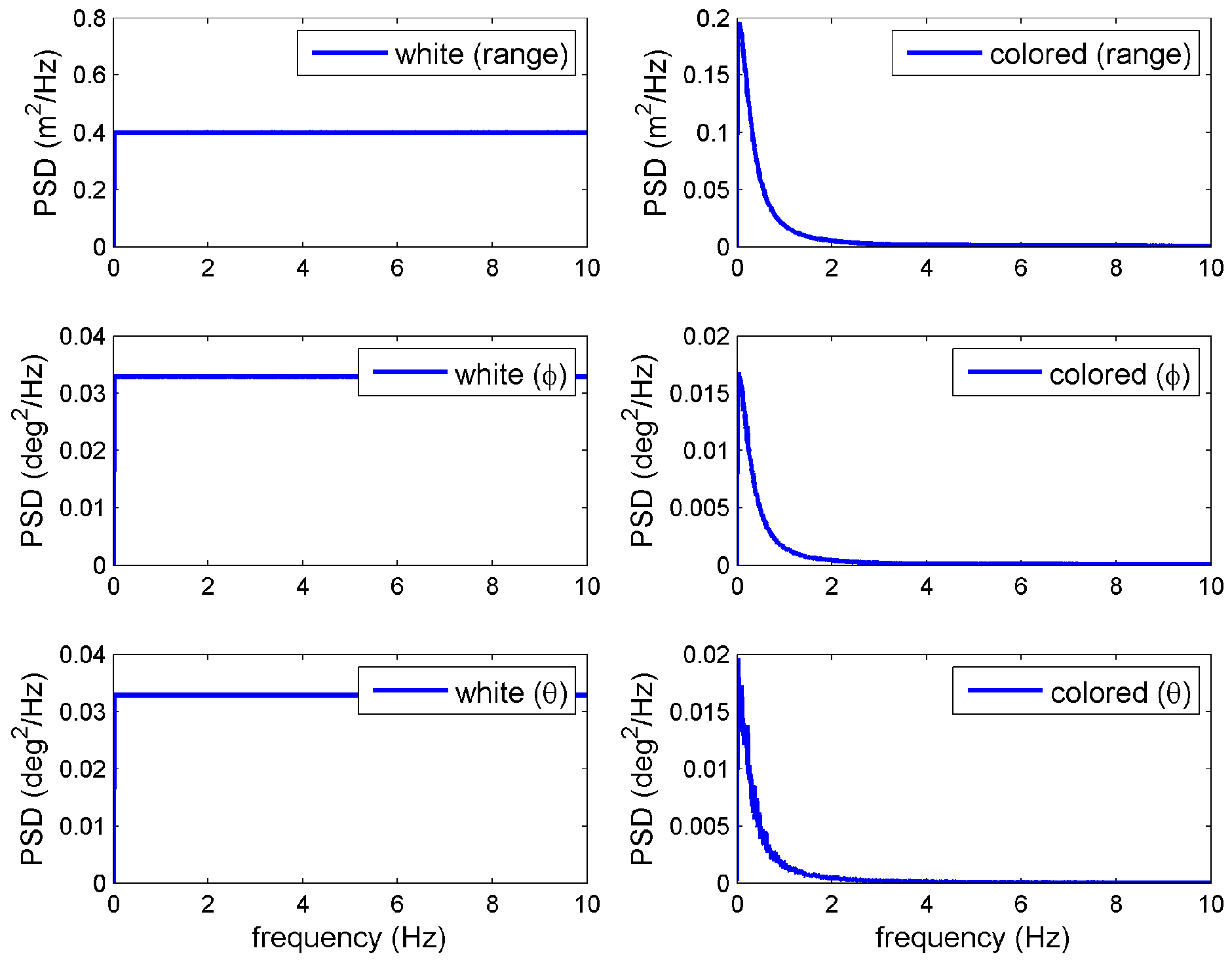
Case 2: Target measurements corrupted by stationary colored (non-white) noise
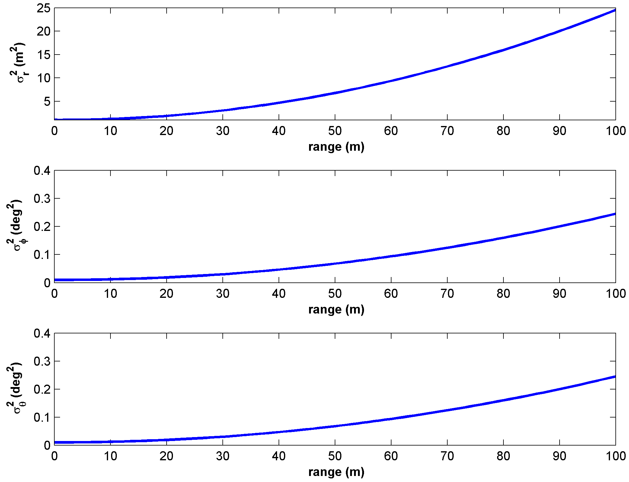
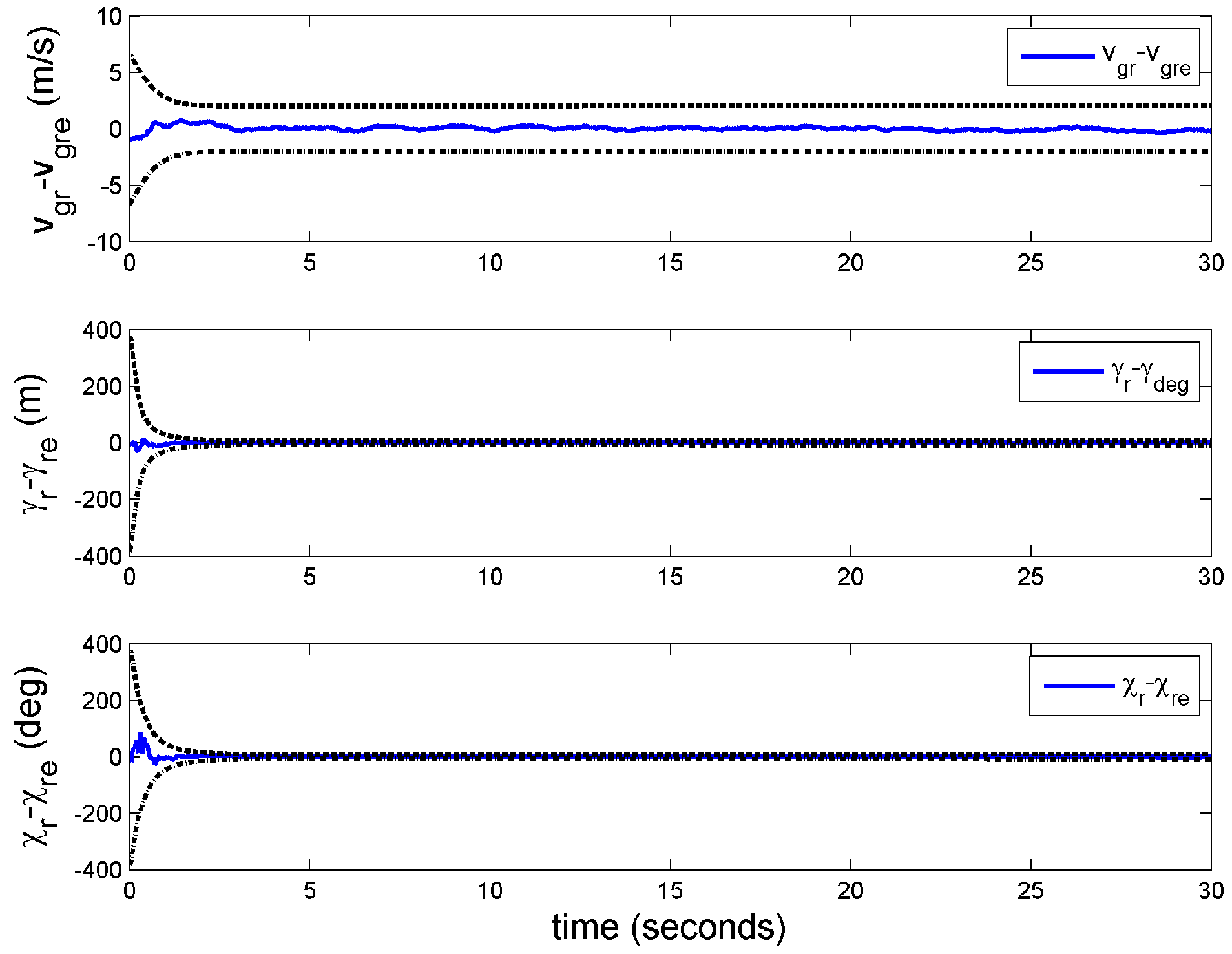
Case 3: Target measurements corrupted by non-stationary white noise with range dependent covariance

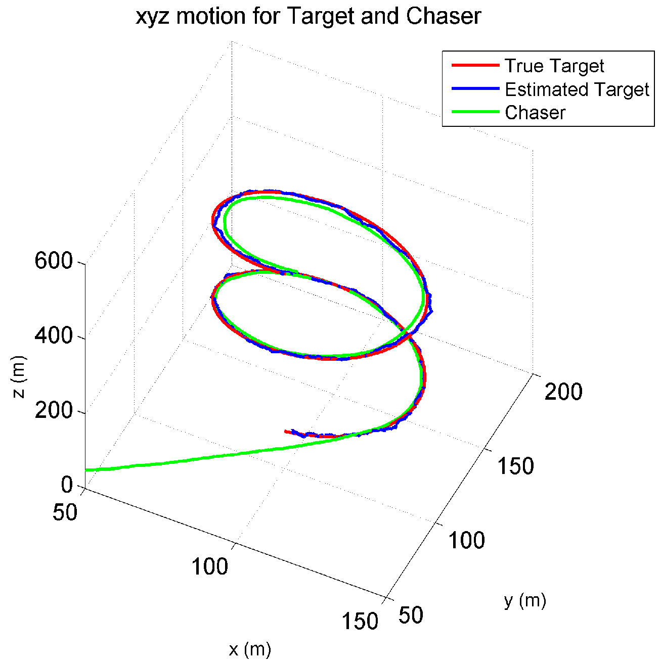
3. Simulation Case Studies
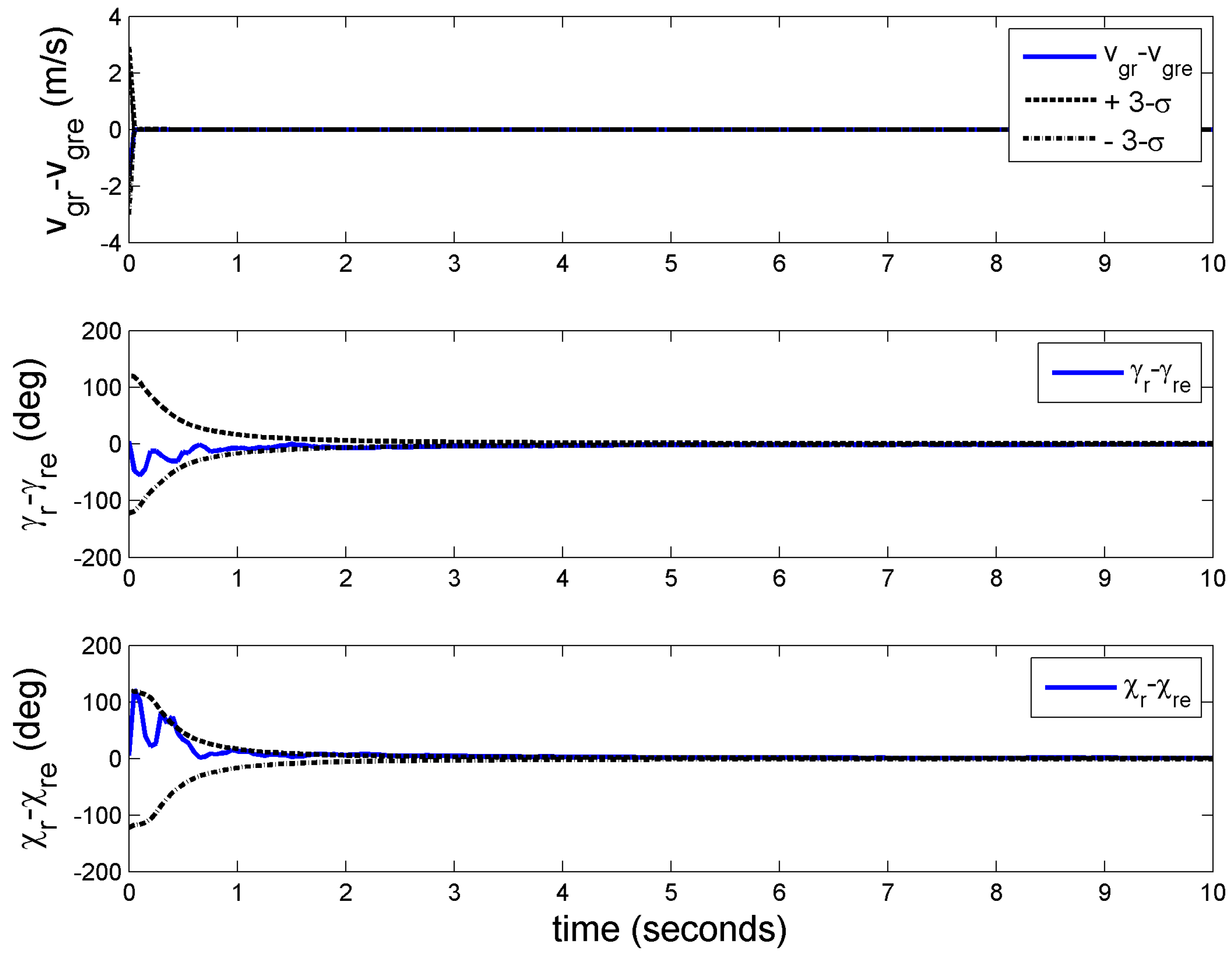
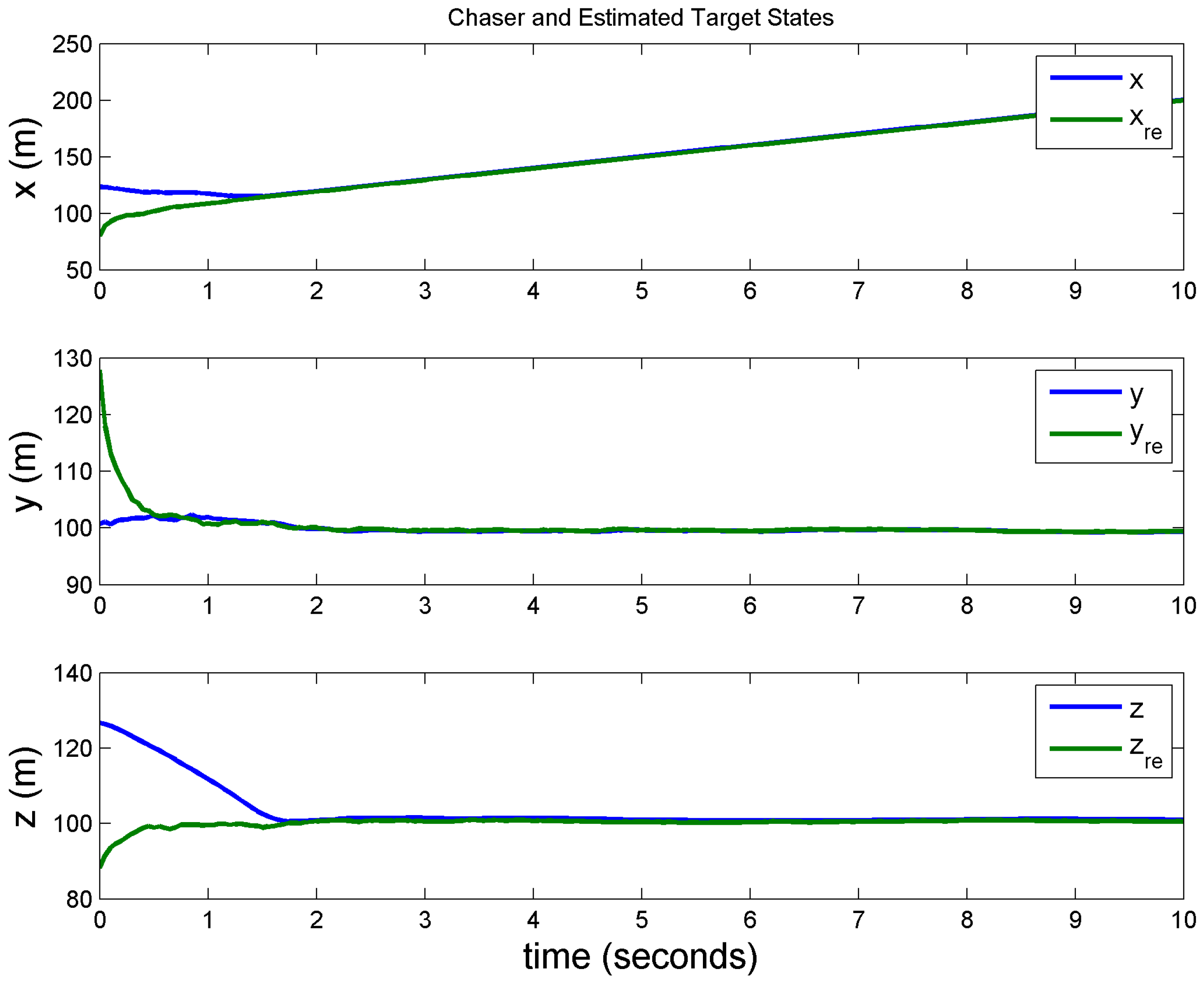
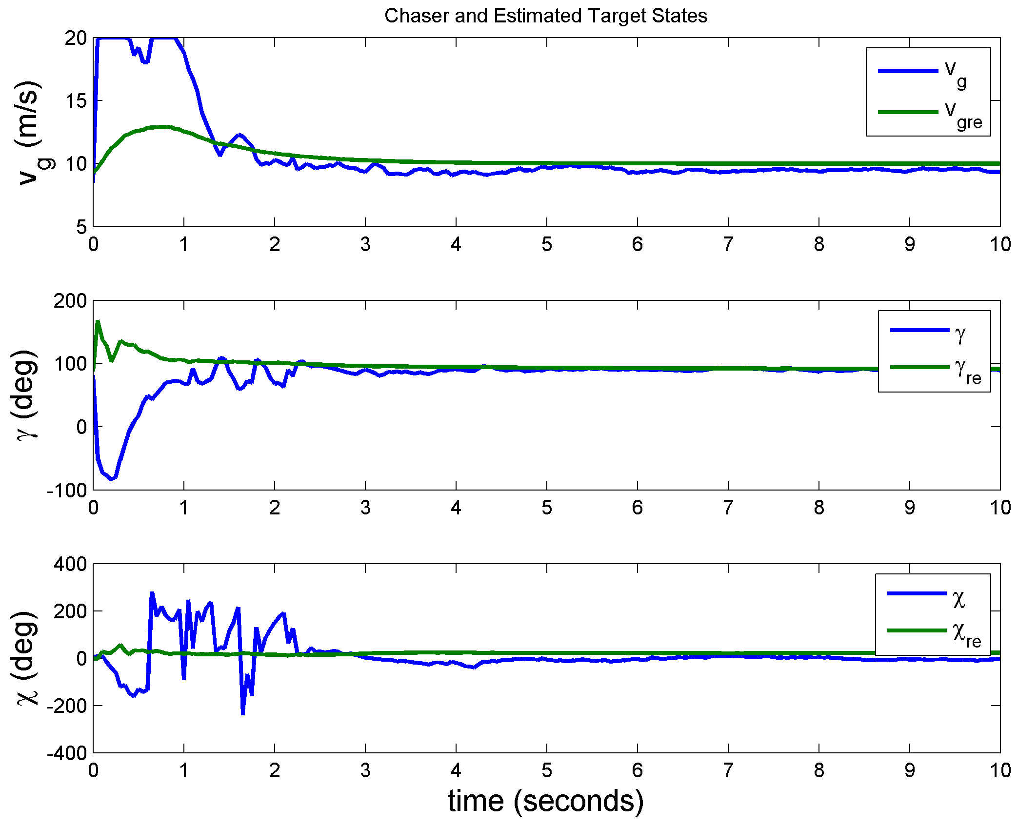
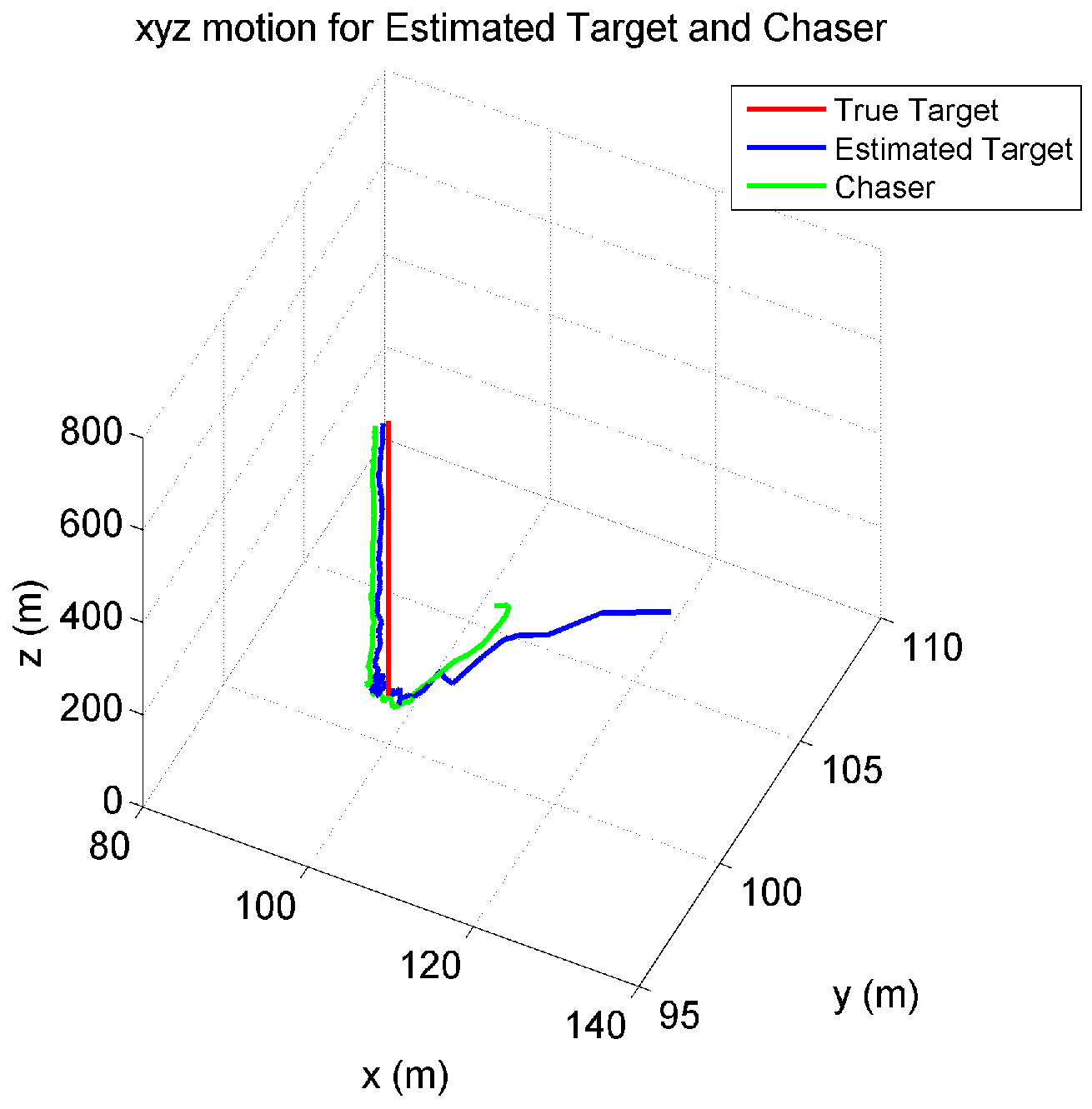
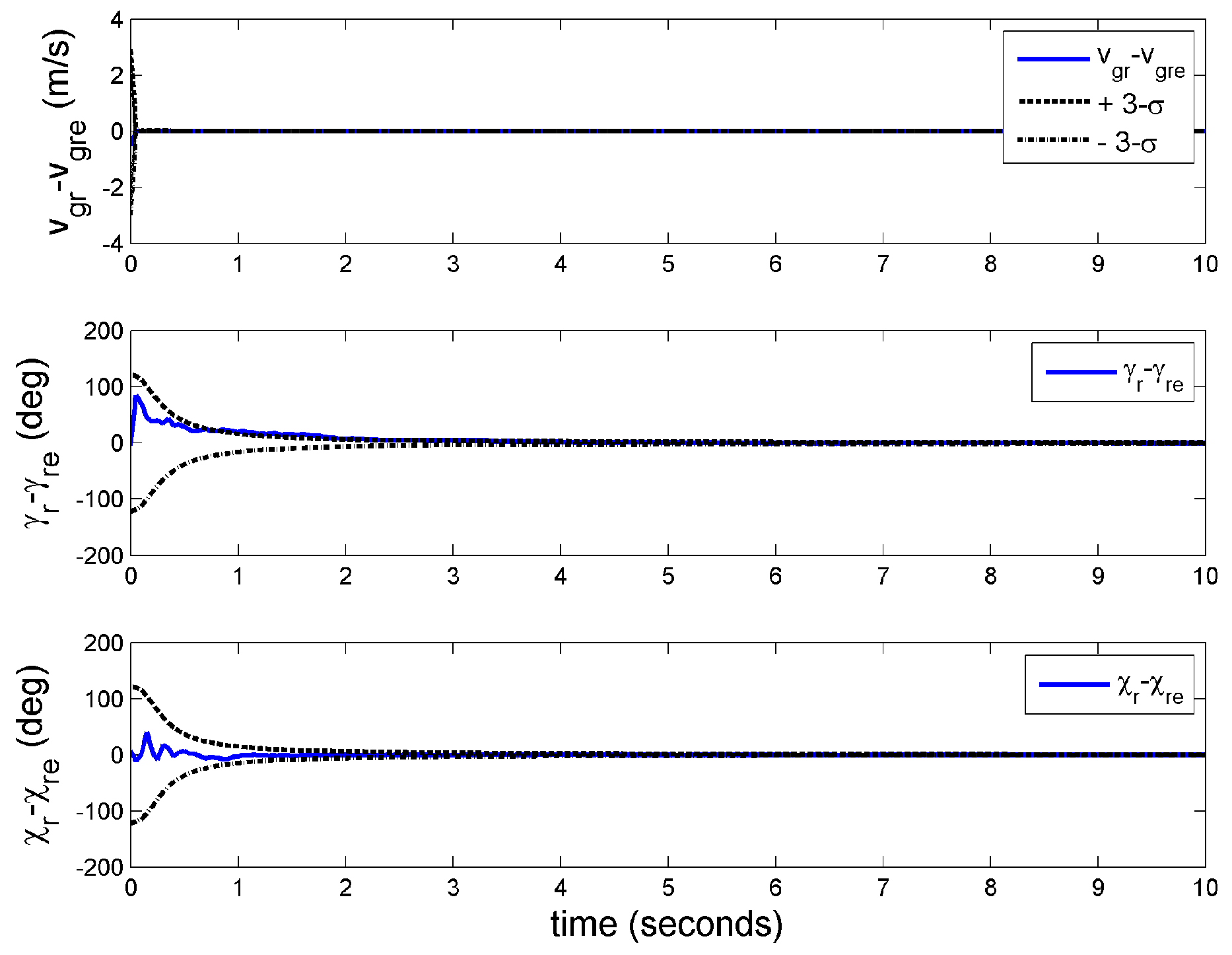
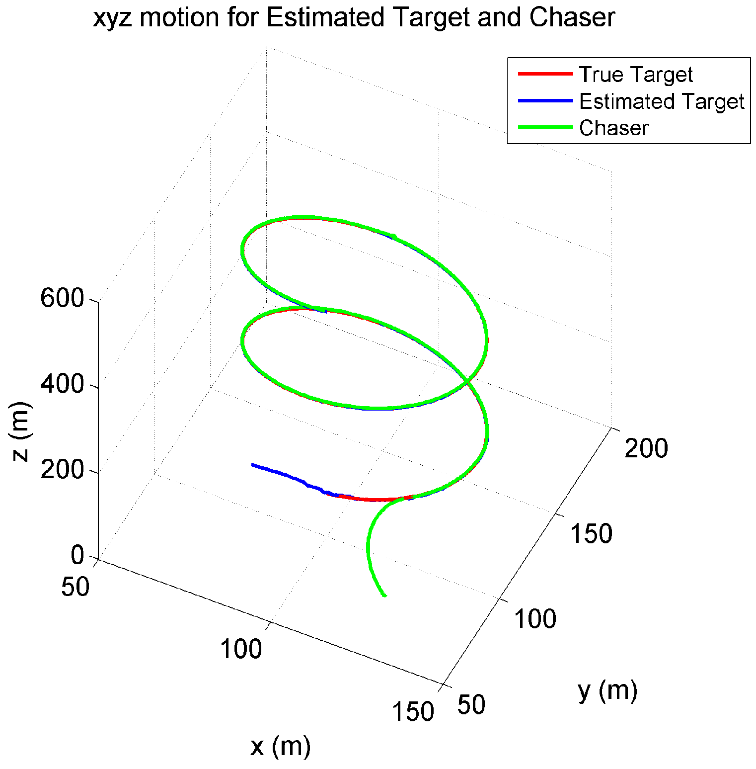
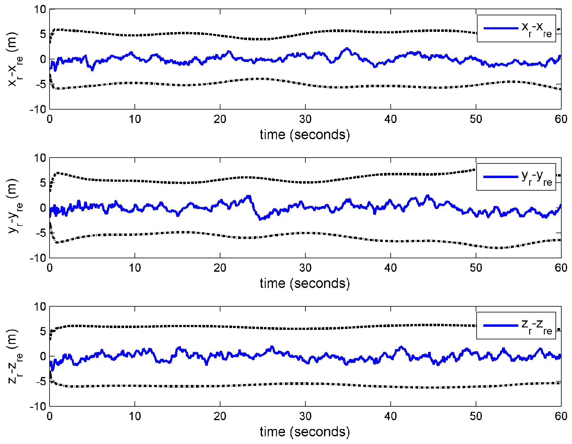
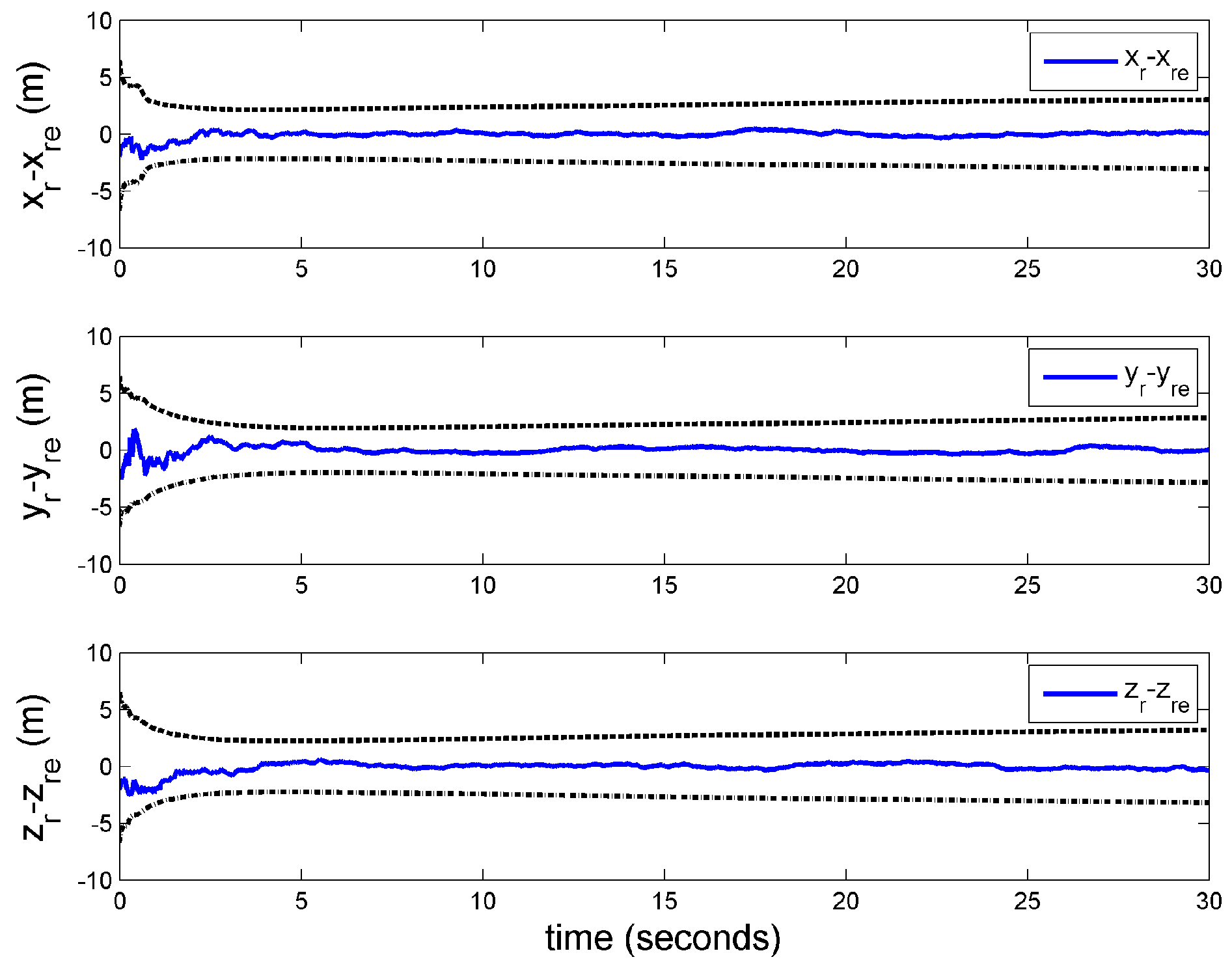
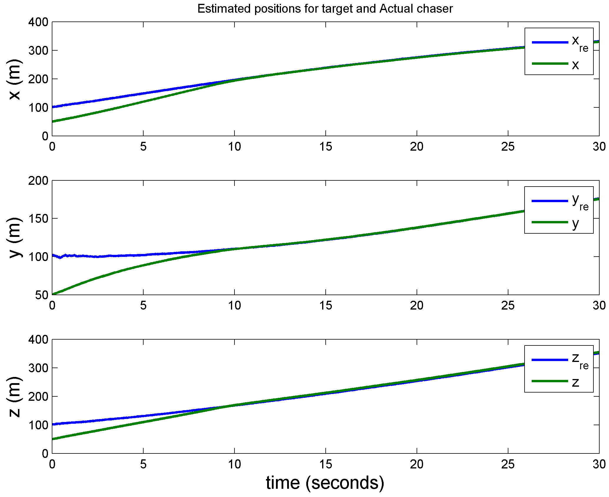
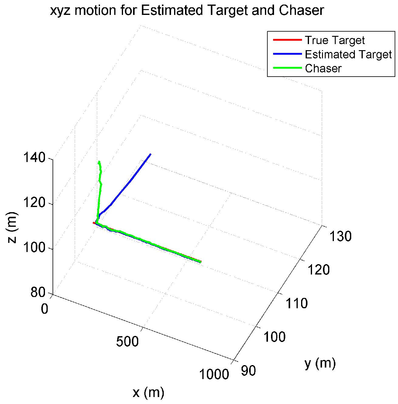
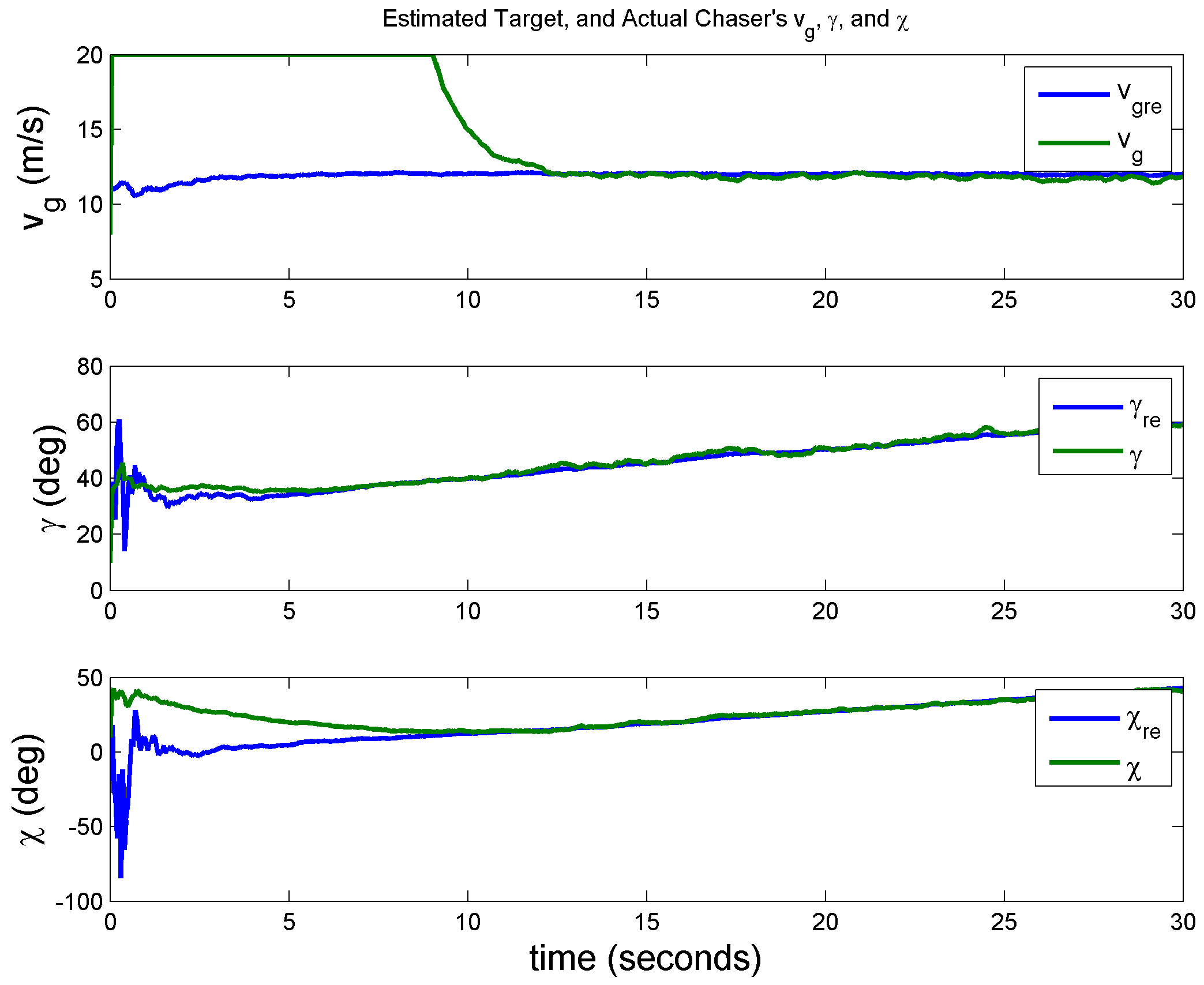
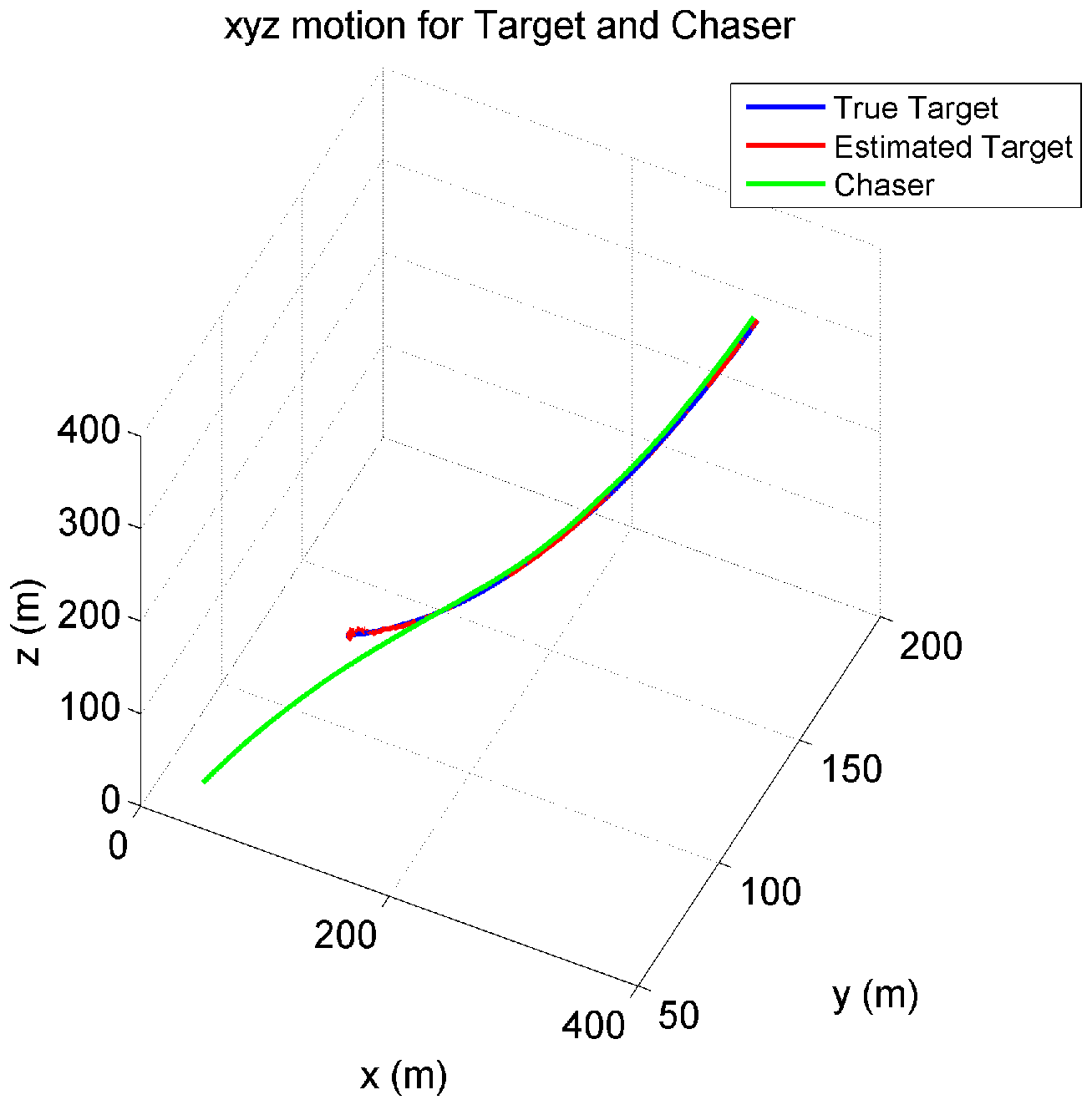
Case 1: Target measurements corrupted by stationary white noise
- A
- Straight line trajectory at constant altitude,
- B
- Straight line trajectory along the z-axis(out-of-plane maneuver), and
- C
- Helical trajectory
- A
- Trajectory at constant altitude: ;
- B
- Trajectory along the z-axis: ;
- C
- Helical Trajectory: .
| Parameter | r | φ | θ |
|---|---|---|---|
| Variance — | |||
| Std. Dev. — σ |


Case 2: Target measurements corrupted by stationary colored (non-white) noise
| Parameter | Value | Unit |
|---|---|---|
| 1 | ||
| 4 | ||


Case 3: Target measurements corrupted by non-stationary white noise with range dependent covariance


4. Conclusions
Author Contributions
Conflicts of Interest
References
- Kalata, P.R. The Tracking Index: A Generalized Parameter for α-β and α-β-γ Target Trackers. IEEE Trans. Aerosp. Electron. Syst. 1984, 20, 174–182. [Google Scholar] [CrossRef]
- Crassidis, J.L.; Junkins, J.L. Optimal Estimation of Dynamic Systems; Chapman and Hall/CRC: Baca Raton, FL, USA, 2004. [Google Scholar]
- Mehrotra, K.; Mahapatra, P.R. A jerk model for tracking highly maneuvering targets. IEEE Trans. Aerosp. Electron. Syst. 1997, 33, 1094–1105. [Google Scholar] [CrossRef]
- Nelson, D.R.; Barber, D.B.; McLain, T.W.; Beard, R.W. Vector Field Path Following for Miniature Air Vehicles. IEEE Trans. Robot. 2007, 23, 519–529. [Google Scholar] [CrossRef]
- Griffiths, S.R. Vector Field Approach for Curved Path Following for Miniature Aerial Vehicles. In Proceeding of the AIAA Guidance, Navigation, and Control Conference and Exhibit, Keystone, CO, USA, 21–24 August 2006.
- Rysdyk, R. Unmanned Aerial Vehicle Path Following for Target Observation in Wind. J. Guid. Control Dyn. 2006, 29, 1092–1100. [Google Scholar] [CrossRef]
- Lawrence, D.; Frew, E.; Pisano, W. Lyapunov Vector Fields for Autonomous Unmanned Aircraft Flight Control. J. Guid. Control Dyn. 2008, 31, 1220–1229. [Google Scholar] [CrossRef]
- Tyler, H.S.; Akella, M.R. Coordinated Standoff Tracking of Moving Targets: Control Laws and Information Architectures. J. Guid. Control Dyn. 2009, 32, 56–69. [Google Scholar]
- Park, S.; Deyst, J.; How, J.P. A New Nonlinear Guidance Logic for Trajectory Tracking. In Proceeding of the AIAA Guidance, Navigation and Control Conference and Exhibit, Providence, RI, USA, 16–19 August 2004.
- Ren, W.; Beard, R.W. Trajectory tracking for Unmanned Air Vehicles with Velocity and Heading Rate Constraints. IEEE Trans. Control Syst. Technol. 2004, 12, 706–716. [Google Scholar] [CrossRef]
- Dubins, L.E. On curves of minimal length with a constraint on average curvature, and with prescribed initial and terminal positions and targets. Am. J. Math. 1957, 79, 497–516. [Google Scholar] [CrossRef]
- Rysdyk, R.; Lum, C.; Vagners, J. Autonomous Orbit Coordination for Two Unmanned Aerial Vehicles. In Proceeding of the AIAA Guidance, Navigation, and Control Conference and Exhibit, San Francisco, CA, USA, 15–18 August 2005.
- Bharadwaj, S.; Rao, A.V.; Mease, K.D. Entry Trajectory Tracking Law via Feedback Linearization. J. Guid. Control Dyn. 1998, 21, 726–732. [Google Scholar] [CrossRef]
- Srivastava, R.; Sarkar, A.K.; Ghose, D.; Gollakota, S. Nonlinear Three Dimensional Composite Guidance Law Based on Feeback Linearization. In AIAA Guidance, Navigation and Control Conference and Exhibit; AIAA: Reston, VA, USA, 2004. [Google Scholar]
- Sarkar, A.K.; Ghose, D. Realistic Pursuer Evader Engagement with Feedback Linearization Based Nonlinear Guidance Law. In Proceeding of the AIAA Guidance, Navigation and Control Conference, 21–24 August 2006.
- Ren, W.; Atkins, E. Nonlinear Trajectory Tracking for Fixed Wing UAVS via Backstepping and Parameter Adaptation. In Proceeding of the AIAA Guidance, Navigation, and Control Conference and Exhibit, San Francisco, CA, USA; 15–18 August 2005. [Google Scholar]
- Jung, D.; Tsiotras, P. Bank-to-Turn Control for a Small UAV using Backstepping and Parameter Adaptation. In Proceeding of the 17th World Congress, The International Federation of Automatic Control, Seoul, South Korea, 6–11 July 2008.
- Lechevin, N.; Rabbath, C.A. Backstepping Guidance for Missile Modeled as Uncertain Time-Varying First-Order Systems. In Proceeding of the American Control Conference, New York, NY, USA, 9–13 July 2007.
- Ahmed, M.; Subbarao, K. Nonlinear 3-D Trajectory Guidance for Unmanned Aerial Vehicles. In Proceeding of the International Conference on Control, Automation, Robotics and Vision, Singapore, 7–10 December 2010.
- Subbarao, K.; Ahmed, M. Nonlinear Guidance and Control Laws for 3-D Target Tracking applied to Unmanned Aerial Vehicles. J. Aerosp. Eng. ASCE 2012. [Google Scholar] [CrossRef]
- Krstic, M.; Kanellakopoulos, I.; Kokotovic, P.V. Nonlinear and Adaptive Control Design; Wiley-Interscience: New York, NY, USA, 1995. [Google Scholar]
- Subbarao, K.; Ahmed, M. 3D Target Tracking by UAVs subject to Measurement Uncertainties. In Proceeding of the IEEE Multi-Conference on Systems and Control, Denver, CO, USA, 28–30 September 2011.
- Bethke, B.; Valenti, M.; How, J. Cooperative Vision Based Estimation and Tracking Using Mulitple UAVs. Lect. Notes Control Inf. Sci. 2007, 369, 179–189. [Google Scholar]
- Ren, W.; Beard, R.W.; Kingston, D.B. Multi-Agent Kalman Consensus with Relative uncertainity. In Proceeding of the American Control Conference, Portland, OR, USA, 8–10 June 2005.
- Olfati-Saber, R. Distributed Kalman filtering for sensor networks. In Proceeding of the IEEE Conference on Decision and Control, New Orleans, LA, USA, 12–14 December 2007; pp. 5492–5498.
- Alighanbari, M.; Ho, J.P. An Unbiased Kalman Consensus Algorithm. In Proceeding of the American Control Conference, Minneapolis, MN, USA, 14–16 June 2006; pp. 3519–3524.
- Garcia-Velo, J.; Walker, B. Aerodynamic parameter estimation for higher performance aircraft using Extended Kalman Filtering. J. Guid. Control Dyn. 1997, 20, 1257–1259. [Google Scholar] [CrossRef]
- Philip, N.K.; Ananthasayanam, M.R. Relative position and attitude estimation and control schemes for the final phase of an autonomous docking mission of spacecraft. Acta Astronaut. 2003, 52, 511–522. [Google Scholar] [CrossRef]
- Kumar, A.; Crassidis, J.L. Colored-Noise Kalman Filter for Vibration Mitigation of Position/Attitude Estimation Systems. In Proceeding of the AIAA Guidance, Navigation, and Control Conference, Hilton Haad, SC, USA, 20–23 August 2007.
- Woffinden, D.C.; Geller, D.K. Relative Angles-Only Navigation and Pose Estimation For Autonomous Orbital Rendezvous. J. Guid. Control Dyn. 2006, 30, 1455–1469. [Google Scholar] [CrossRef]
- Kuhlmann, H. Kalman Filter Colored Measurement Noise for Deformation Analysis. In Proceeding of the 11th FIG Symposium on Deformation Measurements, Ntorini, Greece, 25–28 May 2003.
- Wu, W.R.; Chang, D.C. Maneuvering Target Tracking with Colored Noise. IEEE Trans. Aerosp. Electron. Syst. 1996, 32, 1311–1320. [Google Scholar]
- Tayebi, A.; McGilvray, S. Attitude Stabilization of a VTOL Quadrotor Aircraft. IEEE Trans. Control Syst. Technol. 2006, 14, 562–571. [Google Scholar] [CrossRef]
- Morbidi, F.; Ray, C.; Mariottini, G.L. Cooperative active target tracking for heterogeneous robots with application to gait monitoring. In Proceeding of the IEEE/RSJ International Conference on Intelligent Robots and Systems, San Francisco, CA, USA, 25–30 September 2011; pp. 3608–3613.
© 2016 by the authors; licensee MDPI, Basel, Switzerland. This article is an open access article distributed under the terms and conditions of the Creative Commons by Attribution (CC-BY) license (http://creativecommons.org/licenses/by/4.0/).
Share and Cite
Ahmed, M.; Subbarao, K. Target Tracking in 3-D Using Estimation Based Nonlinear Control Laws for UAVs. Aerospace 2016, 3, 5. https://doi.org/10.3390/aerospace3010005
Ahmed M, Subbarao K. Target Tracking in 3-D Using Estimation Based Nonlinear Control Laws for UAVs. Aerospace. 2016; 3(1):5. https://doi.org/10.3390/aerospace3010005
Chicago/Turabian StyleAhmed, Mousumi, and Kamesh Subbarao. 2016. "Target Tracking in 3-D Using Estimation Based Nonlinear Control Laws for UAVs" Aerospace 3, no. 1: 5. https://doi.org/10.3390/aerospace3010005